Successively Thresholded Domain Boundary Roughening Driven by Pinning Centers and Missing Bonds: Hard-Spin Mean-Field Theory Applied to d=3 Ising Magnets

Abstract

Hard-spin mean-field theory has recently been applied to Ising magnets, correctly yielding the absence and presence of an interface roughening transition respectively in $d=2$ and $d=3$ dimensions and producing the ordering-roughening phase diagram for isotropic and anisotropic systems. The approach has now been extended to the effects of quenched random pinning centers and missing bonds on the interface of isotropic and anisotropic Ising models in $d=3$. We find that these frozen impurities cause domain boundary roughening that exhibits consecutive thresholding transitions as a function interaction of anisotropy. For both missing-bond and pinning-center impurities, for moderately large values the anisotropy, the systems saturate to the ”solid-on-solid” limit, exhibiting a single universal curve for the domain boundary width as a function of impurity concentration.

PACS numbers: 68.35.Dv, 05.50.+q, 64.60.De, 75.60.Ch

I Introduction

Hard-spin mean-field theory HSMFT01 ; HSMFT02 has recently been applied to Ising magnets, correctly yielding the absence and presence of an interface roughening transition respectively in $d=2$ and $d=3$ dimensions and producing the ordering-roughening phase diagram for isotropic and anisotropic systems.HSMFT16 The approach is now extended to the effects of quenched random pinning centers and missing bonds on the interface of isotropic and uniaxially anisotropic Ising models in $d=3$. We find that these frozen impurities cause domain boundary roughening that exhibits consecutive thresholding transitions as a function interaction of anisotropy. We also find that, for both missing-bond and pinning-center impurities, for moderately large values the anisotropy, the systems saturate to the ”solid-on-solid” limit, exhibiting a single universal curve for the domain boundary width as a function of impurity concentration.

Figure 1: A $yz$ plane at temperature $1/J_{xy}=0.1$. Filled and empty circles respectively represent the calculated local magnetizations with $m_{i}>0$ and $m_{i}<0$. The left side is for the pure system, $p=0$. The right side is calculated with quenched random pinning centers with concentration $p=0.24$. Islands that are disconnected from the pinned $z$ boundary plane of their own sign (typically occurring around an opposite pinning center deep inside a bulk phase) do not enter the interface width calculation and are not shown here. Thus, the disconnected pieces seen in this figure are actually part of an overhang, connected to the corresponding $z$ boundary plane via the other $yz$ planes. The dashed lines delimit the domain boundary and the separation between these dashed lines gives the domain boundary width in this $yz$ plane. The same procedure for determining the interface width is also applied to the missing bond systems.

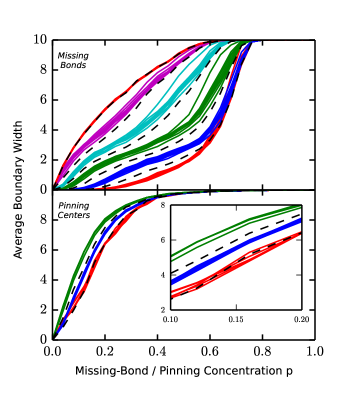
Figure 2: (Color online) Calculated domain boundary widths versus impurity concentration $p$ for different anisotropy $J_{z}/J_{xy}$ values, at temperature $1/J_{xy}=0.1$. In the upper panel, the horizontal axis $p$ is the ratio of the number of missing bonds to the to the total number of bonds when none is missing. In the lower panel, the horizontal axis $p$ is the ratio of the number of pinned sites to the total number of sites. In the upper panel for missing bonds, from the bottom to the top curves, the anisotropies are $J_{z}/J_{xy}=0.1$ to $5.0$ with $0.1$ intervals and $J_{z}/J_{xy}=5.5$ to $10$ with $0.5$ intervals. The dashed curves are calculated with the predicted threshold anisotropy values of $J_{z}/J_{xy}=1,2,3,4,5$. In the lower panel for pinning centers, the anisotropies are $J_{z}/J_{xy}=0.5$ to $2.5$ with $0.1$ intervals. The dashed curves are calculated with the predicted threshold anisotropy values of $J_{z}/J_{xy}=1,2$. Beyond $J_{z}/J_{xy}\simeq 5$ and $2.3$, respectively for missing bonds and pinning centers, the system saturates to the $J_{z}/J_{xy}\rightarrow\infty$ ”solid-on-solid” limit, exhibiting a single universal curve for the domain boundary width as a function of impurity concentration, for all $J_{z}/J_{xy}\gtrsim 5$ and $J_{z}/J_{xy}\gtrsim 2.3$ respectively.

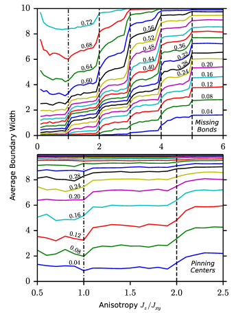
Figure 3: (Color online) Calculated domain boundary widths versus anisotropy $J_{z}/J_{xy}$, at temperature $1/J_{xy}=0.1$. The consecutive curves, bottom to top, are for impurity concentration values of $p=0.04$ to $0.72$ (top panel) and $1$ (bottom panel) with $0.04$ intervals. These values of $p$ are noted next to the curves. In the upper panel, $p$ is the ratio of the number of missing bonds to the to the total number of bonds when none is missing. In the lower panel, $p$ is the ratio of the number of pinned sites to the total number of sites. The curves show the deviations from the isotropic case $J_{z}/J_{xy}=1$ (vertical dash-dotted line) in the directions of strongly coupled planes $J_{z}/J_{xy}>1$ or weakly coupled planes $J_{z}/J_{xy}<1$. The predicted threshold values are shown with the vertical dash-dotted and dashed lines and are well reproduced by the calculated widths. It is clearly seen to the right of this figure that beyond $J_{z}/J_{xy}\simeq 5$ and $2.3$, respectively for missing bonds and pinning centers, the system saturates to the $J_{z}/J_{xy}\rightarrow\infty$ ”solid-on-solid” limit, exhibiting a single universal value for the domain boundary width as a function of impurity concentration, for all $J_{z}/J_{xy}\gtrsim 5$ and $J_{z}/J_{xy}\gtrsim 2.3$ respectively.

II The Anisotropic $d=3$ Ising Model with Impurities and Hard-Spin Mean-Field Theory

II.1 The d=3 Anisotropic Ising Model

The $d=3$ anisotropic Ising model is defined by the Hamiltonian

$$\centering-\beta{\cal H}=J_{xy}\sum_{\left<ij\right>}^{xy}{s_{i}s_{j}}+J_{z}\sum_{\left<ij\right>}^{z}{s_{i}s_{j}},\@add@centering$$ (1)

where at each site $i$ of a cubic lattice, the spin takes on the values $s_{i}=\pm 1$. The first sum is over the nearest-neighbor pairs of sites along the $x$ and $y$ spatial directions and the second sum is over the nearest-neighbor pairs of sites along the $z$ spatial direction. The system has ferromagnetic interactions $J_{xy},J_{z}>0$, periodic boundary conditions in the $x$ and $y$ directions and oppositely fixed boundary conditions at the two terminal planes in the $z$ spatial direction, which yields a domain boundary within the system when in the ordered phase. Thus, the system is generally uniaxially anisotropic. We systematically study the anisotropic $J_{xy}\neq J_{z}$ as well as the isotropic $J_{xy}=J_{z}$ cases.

II.2 Method: Hard-Spin Mean-Field Theory

In our current study, hard-spin mean-field theory HSMFT01 ; HSMFT02 , which has been qualitatively and quantitatively successful in frustrated and unfrustrated, equilibrium and non-equilibrium magnetic ordering problems HSMFT03 ; HSMFT04 ; HSMFT05 ; HSMFT06 ; HSMFT07 ; HSMFT08 ; HSMFT09 ; HSMFT10 ; HSMFT11 ; HSMFT12 ; HSMFT13 ; HSMFT14 ; HSMFT15 ; HSMFT16 ; HSMFT17 , including recently the interface roughening transition HSMFT16 , is used to study the roughening of an interface by quenched random pinning center sites or missing bonds. The self-consistency equations of hard-spin mean-field theory HSMFT02 are

$$\centering m_{i}=\sum_{\left\{s_{j}\right\}}\left[\left(\prod_{j}{\frac{1+m_{j}s_{j}}{2}}\right)\tanh\left({\sum_{j}J_{ij}s_{j}}\right)\right],\@add@centering$$ (2)

where $m_{i}=<s_{i}>$ is the local magnetization at site $i$, the sum $\{s_{j}\}$ is over all possible values of the spins $s_{j}$ at the nearest-neighbor sites $j$ to site $i$, and $m_{j}$ are the magnetizations at the nearest-neighbor sites. These coupled equations for all sites are solved by local numerical iteration, in a $10\times 10\times 10$ system.

III Domain Boundary Widths

III.1 Determination of the Domain Boundary Width

In our study, the domain boundary is roughened in two ways: (1) Magnetic impurities are included in the system by pinning randomly chosen sites to $s_{i}=+1$ or to $s_{i}=-1$. The impurity concentration $p$ in this case is the ratio of the number of pinned sites to the total number of sites. The numbers of $+1$ and $-1$ pinned sites are fixed to be equal, to give both domains an equal chance to advance over its counter. (2) Missing bonds are created by removing randomly chosen bonds. In this case, the concentration $p$ is given by the ratio of the number of removed bonds to the total number of bonds when none is missing.

The domain boundary width is calculated by first considering each $yz$ plane. The boundary width in each $yz$ plane is calculated by counting the number of sites, in the $z$ direction, between the two furthest opposite magnetizations in the plane (Fig. 1). This number is averaged over all the $yz$ planes. The result is then averaged over $100$ independent realizations of the quenched randomness. We have checked that our results are robust with respect to varying the number of independent realizations of the quenched randomness, as shown below.

III.2 Impurity Effects on
the Domain Boundary Width

Our calculated domain boundary widths, as a function of impurity (i.e., missing-bond or pinned-site) concentration $p$ at temperature $1/J_{xy}=0.1$, are shown in Fig. 2. The different curves are for different interaction anisotropies $J_{z}/J_{xy}$. In the lower panel for pinning-center impurity, the domain boundary roughens with the introduction of infinitesimal impurity, for all anisotropies: The curves have finite slope at the pure system. In the upper panel for missing-bond impurity, the domain boundary roughens with the introduction of infinitesimal impurity for strongly coupled planes $J_{z}/J_{xy}>2.5$, whereas for weakly coupled planes $J_{z}/J_{xy}<2.5$, it is seen that infinitesimal or small impurity has essentially no effect on the flat domain boundary. In the latter cases, the curves reach the pure system with zero slope.

For both missing-bond and pinning-center impurities, for moderately large values of $J_{z}/J_{xy}$, we find (Figs. 2 and 3) that the systems saturate to the $J_{z}/J_{xy}\rightarrow\infty$ ”solid-on-solid” limit sons . Thus, the systems exhibit a single universal curve for the domain boundary width as a function of impurity concentration, onwards from all moderately large values of $J_{z}/J_{xy}$.

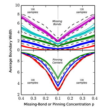
Figure 4: (Color online) Calculated domain boundary widths versus impurity concentration $p$ for different anisotropy $J_{z}/J_{xy}$ values, at temperature $1/J_{xy}=0.1$. These curves are obtained by averaging over $100$ (left panels) and $120$ (right panels) independent realizations of the quenched randomness. In the upper panel, the horizontal axis $p$ is the ratio of the number of missing bonds to the to the total number of bonds when none is missing. In the lower panel, the horizontal axis $p$ is the ratio of the number of pinned sites to the total number of sites. In the upper panel for missing bonds, from the bottom to the top curves, the anisotropies are $J_{z}/J_{xy}=0.1$ to $5.0$ with $0.1$ intervals. The dashed curves are calculated with the predicted threshold anisotropy values of $J_{z}/J_{xy}=1,2,3,4,5$. In the lower panel for pinning centers, the anisotropies are $J_{z}/J_{xy}=0.5$ to $2.3$ with $0.1$ intervals. The dashed curves are calculated with the predicted threshold anisotropy values of $J_{z}/J_{xy}=1,2$. Comparison of the left and right panels shows that our results are robust with respect to varying the number of independent realizations of the quenched randomness.

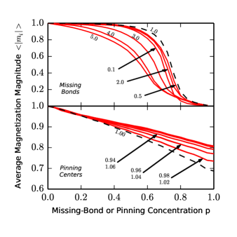
Figure 5: (Color online) Calculated local magnetization magnitudes $<|m_{i}|>$ averaged across the system versus impurity concentration $p$ for different anisotropy $J_{z}/J_{xy}$ values, at temperature $1/J_{xy}=0.1$. In the upper panel, the horizontal axis $p$ is the ratio of the number of missing bonds to the to the total number of bonds when none is missing. In the lower panel, the horizontal axis $p$ is the ratio of the number of pinned sites to the total number of sites. In each panel, the dashed curve corresponds to the isotropic case $J_{z}/J_{xy}=1$. The full curves are for the anisotropic cases. Some of the $J_{z}/J_{xy}$ values for the anisotropic cases are indicated next to the corresponding curves. Note that the average magnetization magnitude curve of the isotropic case constitutes an upper boundary to the curves of the anisotropic cases for the missing bonds system (upper panel). The average magnetization magnitude curve of the isotropic case constitutes a lower boundary to the curves of the anisotropic cases for the pinning center system (lower panel). This is understandable by the fact that missing bonds weaken the connectivity and therefore the magnetization of the system, whereas pinning centers constitute a strong aligning field to their neighboring spins. In curves in the lower panel, the deviation from the isotropic case is symmetric, so that each curve corresponds to two values of the anisotropy $J_{z}/J_{xy}$ which are above and below the isotropic case $J_{z}/J_{xy}=1$.

III.3 Successive Roughening Thresholds

A bunching of the curves is visible, in the domain-boundary width curves in Fig. 2, especially in the upper panel for missing-bond impurity. This corresponds to a thresholded domain boundary roughening, controlled by the interaction anisotropy. This effect is also visible in Fig. 3, by the steps in the curves which give the domain boundary widths as a function of the interaction anisotropy $J_{z}/J_{xy}$ for different impurity concentrations $p$, at temperature $1/J_{xy}=0.1$. We have checked that our results are robust with respect to varying the number of independent realizations of the quenched randomness. This is shown in Fig. 4.

Thresholded domain boundary roughening can be understood by considering the effect of increasing the anisotropy. We first discuss the case of missing-bond impurity. Upon increasing $J_{z}$, for what value of $J_{z}$ will a spin flip, e.g., from +1 to -1, thereby increasing the domain boundary width (directly and/or by inducing a flip cascade)? Increasing $J_{z}$ can flip a spin and increase the width only if one of its bonds in the $\pm z$ direction is missing and the non-missing bond connects to a -1 spin. This flip will then happen for $J_{z}=(q-q^{\prime})J_{xy}$, where $(q,q^{\prime})$ are the numbers of $xy$ neighbors bonded to the flipping spin that are respectively +1, -1. The possible values are $(q,q^{\prime})=(4,0),(3,0),(2,0),(1,0),(3,1),(2,1)$, giving the threshold values of $J_{z}/J_{xy}=1,2,3,4$, in fact calculationally seen in the top panels of Figs. 2 and 3. Furthermore, the simultaneous flip of two neighboring spins gives the threshold value of $J_{z}/J_{xy}=5$, also calculationally seen in the top panels of Figs. 2 and 3. Beyond $J_{z}/J_{xy}=5$, the system saturates to the $J_{z}/J_{xy}\rightarrow\infty$ ”solid-on-solid” limit sons , exhibiting a single universal curve for the domain boundary width as a function of impurity concentration, for all $J_{z}/J_{xy}\gtrsim 5$.

We now discuss the case of pinned-site impurity. We again consider the effect of increasing $J_{z}$ and investigate the value of $J_{z}$ that will flip the spin, e.g., from +1 to -1, thereby increasing the domain boundary width (again, directly and/or by inducing a flip cascade). Increasing $J_{z}$ can flip this spin only if both of its neighbors in the $\pm z$ direction are -1, with one of these being part of a disconnected island seeded by a pinning center. This flip will then happen for $2J_{z}=(q-q^{\prime})J_{xy}$, where again $q$ and $q^{\prime}$ are the numbers of $xy$ neighbors bonded to the flipping spin that are respectively +1 and -1. The possible values are $(q,q^{\prime})=(4,0),(3,1)$, giving the threshold values of $J_{z}/J_{xy}=1,2$, calculationally seen in the bottom panels of Figs. 2 and 3. Beyond $J_{z}/J_{xy}\simeq 2.3$, the system saturates to the $J_{z}/J_{xy}\rightarrow\infty$ ”solid-on-solid” limit sons , exhibiting a single universal curve for the domain boundary width as a function of impurity concentration, for all $J_{z}/J_{xy}\gtrsim 2.3$.

On a similar vein, in the limit of $xy$ planes weakly coupled due to low $J_{z}/J_{xy}$ and high concentration of missing bonds, the domain boundary gains by the intermediacy of sending overhangs in the lateral $x$ and $y$ directions, eventually covering the whole system via randomly magnetized $xy$ planes. In this case, the spin is flipped by the effect of $J_{xy}$ upon decreasing $J_{z}$. This flip occurs at $2J_{z}=(q-q^{\prime})J_{xy}$, where $(q,q^{\prime})$ has to be such that $J_{z}/J_{xy}$ is low. Thus, $(q,q^{\prime})=(2,1)$. (Other pairs of values, (3,0) and (1,0) do not contribute to this spread of overhangs.) Indeed, in Fig. 3, a rise in the domain for decreasing $J_{z}<0.5$ is seen at high missing bond concentration.

The curves in Fig. 3 are domain boundary widths that are affected by complicated (due to the random geometric distribution of the impurities) cascades of flips of groups of spins, occurring continuously as the interaction anisotropy is changed. The arguments given above are for single-spin flips, which strongly affect the boundary width at the specific anisotropy ratios.

We note that since in this system the interactions acting on a given spin $s_{i}$ can be competing, due to the presence of the interface or of a neighboring pinning center, all of the local magnetizations $m_{i}=<s_{i}>$, where the averaging is thermal, are not saturated even at low temperatures. Such an effect has been seen down to zero temperature in other systems with competing interactions, as for example shown in Fig. 3 of Ref. Yesilleten . In our present study, the calculated magnitudes of the local magnetizations averaged across our current system, $<|m_{i}|>$, are given in Fig. 5 and show this unsaturation.

IV Conclusion

The effects of quenched random pinning centers and missing bonds on the interface of isotropic and uniaxially anisotropic Ising models in $d=3$ have been investigated by hard-spin mean-field theory. We find that the frozen impurities cause domain boundary roughening that exhibits consecutive thresholding transitions as a function interaction of anisotropy $J_{z}/J_{xy}$. The numerical results, showing the thresholding transitions as the bunching of domain boundary width versus impurity concentration curves (Fig. 2) and steps in the domain boundary width versus anisotropy curves (Fig. 3) agree with our spin-flip arguments at the interface. The threshold effect should be fully observable in experimental magnetic samples with good crystal structure and point impurities. For both missing-bond and pinning-center impurities, for moderately large values of $J_{z}/J_{xy}$, the systems saturate to the $J_{z}/J_{xy}\rightarrow\infty$ ”solid-on-solid” limit, thus exhibiting a single universal curve for the domain boundary width as a function of impurity concentration, onwards from all moderately large values of $J_{z}/J_{xy}$.

- (1) R. R. Netz and A. N. Berker, Phys. Rev. Lett. 66, 377 (1991).
- (2) R. R. Netz and A. N. Berker, J. Appl. Phys. 70, 6074 (1991).
- (3) T. Çağlar and A. N. Berker, Phys. Rev. E 84, 051129 (2011).
- (4) J. R. Banavar, M. Cieplak, and A. Maritan, Phys. Rev. Lett. 67, 1807 (1991).
- (5) R. R. Netz and A. N. Berker, Phys. Rev. Lett. 67, 1808 (1991).
- (6) R. R. Netz, Phys. Rev. B 46, 1209 (1992).
- (7) R. R. Netz, Phys. Rev. B 48, 16113 (1993).
- (8) A. N. Berker, A. Kabakçıoğlu, R. R. Netz, and M. C. Yalabık, Turk. J. Phys. 18, 354 (1994).
- (9) A. Kabakçıoğlu, A. N. Berker, and M. C. Yalabık, Phys. Rev. E 49, 2680 (1994).
- (10) E. A. Ames and S. R. McKay, J. Appl. Phys. 76, 6197 (1994).
- (11) G. B. Akgüç and M. C. Yalabık, Phys. Rev. E 51, 2636 (1995).
- (12) J. E. Tesiero and S. R. McKay, J. Appl. Phys. 79, 6146 (1996).
- (13) J. L. Monroe, Phys. Lett. A 230, 111 (1997).
- (14) A. Pelizzola and M. Pretti, Phys. Rev. B 60, 10134 (1999).
- (15) A. Kabakçıoğlu, Phys. Rev. E 61, 3366 (2000).
- (16) H. Kaya and A. N. Berker, Phys. Rev. E 62, R1469 (2000); also see M. D. Robinson, D. P. Feldman, and S. R. McKay, Chaos 21, 037114 (2011).
- (17) O. S. Sarıyer, A. Kabakçıoğlu, and A. N. Berker, Phys. Rev. E 86, 041107 (2012).
- (18) R. H. Swendsen, Phys. Rev. B 15, 689 (1977).
- (19) D. Yeşilleten and A. N. Berker, Phys. Rev. Lett. 78, 1564 (1997).