A Possible Implementation of a Direct Coupling Coherent Quantum Observer

Abstract

This paper considers the problem of implementing a previously proposed direct coupling quantum observer for a closed linear quantum system. This observer is shown to be able to estimate some but not all of the plant variables in a time averaged sense. The paper proposes a possible experimental implementation of the observer plant system using a non-degenerate parametric amplifier.

I Introduction

A number of papers have recently considered the problem of constructing a coherent quantum observer for a quantum system; see [1, 2, 3]. In the coherent quantum observer problem, a quantum plant is coupled to a quantum observer which is also a quantum system. The quantum observer is constructed to be a physically realizable quantum system so that the system variables of the quantum observer converge in some suitable sense to the system variables of the quantum plant. The papers [4, 5, 6, 7] considered the problem of constructing a direct coupling quantum observer for a given quantum system.

In the papers [1, 2, 4, 6], the quantum plant under consideration is a linear quantum system. In recent years, there has been considerable interest in the modeling and feedback control of linear quantum systems; e.g., see [8, 9, 10]. Such linear quantum systems commonly arise in the area of quantum optics; e.g., see [11, 12]. For such linear quantum system models, an important class of quantum control problems are referred to as coherent quantum feedback control problems; e.g., see [8, 9, 13, 14, 15, 16, 17, 18]. In these coherent quantum feedback control problems, both the plant and the controller are quantum systems and the controller is typically to be designed to optimize some performance index. The coherent quantum observer problem can be regarded as a special case of the coherent quantum feedback control problem in which the objective of the observer is to estimate the system variables of the quantum plant.

In this paper, we consider the situation as in papers [4, 5, 6, 7] in which there is only direct coupling between quantum plant and the quantum observer. In these papers, both the quantum plant and the quantum observer are assumed to be closed quantum systems which means that they are not subject to quantum noise and are purely deterministic systems. This leads to an observer structure of the form shown in Figure 1. In these papers, it is shown that a quantum observer can be constructed to estimate some but not all of the system variables of the quantum plant. Also, the observer variables converge to the plant variables in a time averaged sense rather than a quantum expectation sense such as considered in the papers [1, 2].

Figure 1: Coherent Observer Structure with Direct Coupling.

In this paper, we concentrate on the result presented in [4] for the case in which the quantum plant is a single quantum harmonic oscillator and the quantum observer is a single quantum harmonic oscillator. For this case, we show that a possible experimental implementation of the augmented quantum plant and quantum observer system may be constructed using a non-degenerate parametric amplifier (NDPA) which is coupled to a beamsplitter by suitable choice of the amplifier and beamsplitter parameters.

II Quantum Linear Systems

In this section, we describe the class of closed linear quantum systems under consideration; see also [8, 19, 15, 4, 6]. We consider linear non-commutative systems of the form

$$\dot{x}(t) = Ax(t);\quad x(0)=x_{0}$$ (1)

where $A$ is a real matrix in $\mathbb{R}^{n\times n}$, and $x(t)=[\begin{array}[]{ccc}x_{1}(t)&\ldots&x_{n}(t)\end{array}]^{T}$ is a vector of self-adjoint possibly non-commutative system variables; e.g., see [8]. Here $n$ is assumed to be an even number and $\frac{n}{2}$ is the number of modes in the quantum system.

The initial system variables $x(0)=x_{0}$ are assumed to satisfy the commutation relations

$$[x_{j}(0),x_{k}(0)]=2i\Theta_{jk},\ \ j,k=1,\ldots,n,$$ (2)

where $\Theta$ is a real antisymmetric matrix with components $\Theta_{jk}$. Here, the commutator is defined by $[A,B]=AB-BA$. In the case of a single degree of freedom quantum particle, $x=(x_{1},x_{2})^{T}$ where $x_{1}=q$ is the position operator, and $x_{2}=p$ is the momentum operator. The commutation relations are $[q,p]=2i$. Here, the matrix $\Theta$ is assumed to be of the form $\Theta={\rm diag}(J,J,\ldots,J)$ where $J$ denotes the real skew-symmetric $2\times 2$ matrix

$$J=\left[\begin{array}[]{cc}0&1\\ -1&0\end{array}\right].$$

A linear quantum system (1) is said to be physically realizable if it ensures the preservation of the canonical commutation relations (CCRs):

$$x(t)x(t)^{T}-(x(t)x(t)^{T})^{T}=2i\Theta\ \mbox{for all }t\geq 0.$$

This holds when the system (1) corresponds to a collection of closed quantum harmonic oscillators; see [8]. Such quantum harmonic oscillators are described by a quadratic Hamiltonian $\mathcal{H}=\frac{1}{2}x^{T}Rx$, where $R$ is a real symmetric matrix.

In the proposed direct coupling coherent quantum observer, the quantum plant is a single quantum harmonic oscillator which is a linear quantum system of the form (1) described by the non-commutative differential equation

$$\dot{x}_{p}(t) = A_{p}x_{p}(t);\quad x_{p}(0)=x_{0p};$$

$$z_{p}(t) = C_{p}x_{p}(t)$$ (3)

where $z_{p}(t)$ denotes the vector of system variables to be estimated by the observer and $A_{p}\in\mathbb{R}^{2\times 2}$, $C_{p}\in\mathbb{R}^{1\times 2}$. It is assumed that this quantum plant corresponds to a plant Hamiltonian $\mathcal{H}_{p}=\frac{1}{2}x_{p}^{T}R_{p}x_{p}$. Here $x_{p}=\left[\begin{array}[]{l}q_{p}\\ p_{p}\end{array}\right]$ where $q_{p}$ is the plant position operator and $p_{p}$ is the plant momentum operator.

We now describe the linear quantum system of the form (1) which will correspond to the quantum observer; see also [8, 19, 15]. This system is described by a non-commutative differential equation of the form

$$\dot{x}_{o}(t) = A_{o}x_{o}(t);\quad x_{o}(0)=x_{0o};$$

$$z_{o}(t) = C_{o}x_{o}(t)$$ (4)

where the observer output $z_{o}(t)$ is the observer estimate and $A_{o}\in\mathbb{R}^{2\times 2}$, $C_{o}\in\mathbb{R}^{1\times 2}$. Here $x_{o}=\left[\begin{array}[]{l}q_{o}\\ p_{o}\end{array}\right]$ where $q_{o}$ is the observer position operator and $p_{o}$ is the observer momentum operator. We assume that the plant variables commute with the observer variables. The system dynamics (4) are determined by the observer system Hamiltonian which is a self-adjoint operator on the underlying Hilbert space for the observer. For the quantum observer under consideration, this Hamiltonian is given by a quadratic form: $\mathcal{H}_{o}=\frac{1}{2}x_{o}^{T}R_{o}x_{o}$, where $R_{o}$ is a real symmetric matrix. Then, the corresponding matrix $A_{o}$ in (4) is given by

$$A_{o}=2JR_{o}.$$ (5)

In addition, we define a coupling Hamiltonian which determines the coupling between the quantum plant and the quantum observer:

$$\mathcal{H}_{c}=x_{p}^{T}R_{c}x_{o}.$$

III Direct Coupling Distributed Coherent Quantum Observer

Following [4, 6], we assume that $A_{p}=0$ in (3). This corresponds to $R_{p}=0$ in the plant Hamiltonian. It follows from (3) that the plant system variables $x_{p}(t)$ will remain fixed if the plant is not coupled to the observer. However, when the plant is coupled to the quantum observer this will no longer be the case. In addition, we construct the observer as in [4] so that

$$R_{o}>0\mbox{ and }R_{c}=C_{p}^{T}\beta$$ (6)

where

$$\beta\in\mathbb{R}^{1\times 2}\mbox{ and }C_{o}R_{o}^{-1}\beta^{T}=-1.$$ (7)

With this construction of the quantum observer, the following result was established in [4].

Theorem 1

Consider a quantum plant of the form (3) where $A_{p}=0$. Then the matrices $R_{o}>0$, $R_{c}$, $C_{o}$ satisfying the conditions (6), (7) will define direct coupled quantum observer such that for the resulting augmented plant-observer system, the quantity $z_{p}(t)$ is constant and

$$\lim_{T\rightarrow\infty}\frac{1}{T}\int_{0}^{T}(z_{p}-z_{o}(t))dt=0.$$ (8)

IV A Possible Implementation of the Plant Observer System

In this section, we describe one possible experimental implementation of the plant-observer system given in the previous section. The plant-observer system is a linear quantum system of the form (1) with Hamiltonian $\mathcal{H}=\frac{1}{2}x^{T}Rx=\frac{1}{2}x_{o}^{T}R_{o}x_{o}+x_{p}^{T}R_{c}x_{o}$ where the conditions (6), (7) are satisfied. In particular, we assume $R_{o}=2\omega_{o}I>0$ and hence

$$\mathcal{H}=\omega_{o}x_{o}^{T}x_{o}+x_{p}^{T}C_{p}^{T}\beta x_{o}.$$ (9)

Also, the condition (7) becomes

$$C_{o}\beta^{T}+2\omega_{o}=0.$$ (10)

In order to construct a linear quantum system with a Hamiltonian of this form, we consider an NDPA coupled to a beamsplitter as shown schematically in Figure 2; e.g., see [12].

Figure 2: NDPA coupled to a beamsplitter.

A linearized approximation to the NDPA is defined by a quadratic Hamiltonian of the form

$$\mathcal{H}_{1}=\frac{\imath}{2}\left(\epsilon a^{*}b^{*}-\epsilon^{*}ab\right)+\omega_{o}b^{*}b$$

where $a$ is the annihilation operator corresponding to the first mode of the NDPA and $b$ is the annihilation operator corresponding to the second mode of the NDPA. These modes will be assumed to be of the same frequency but with a different polarization with $a$ corresponding to the quantum plant and $b$ corresponding to the quantum observer. Also, $\epsilon$ is a complex parameter defining the level of squeezing in the NDPA and $\omega_{o}$ is the detuning frequency of the $b$ mode in the NDPA. The $a$ mode in the NDPA is assumed to be tuned. In addition, the NDPA is defined by the vector of coupling operators $L=\left[\begin{array}[]{l}\sqrt{\gamma}a\\ \sqrt{\gamma}b\end{array}\right]$. Here $\gamma>0$ is a scalar parameter determined by the reflectance of the mirrors in the NDPA.

From the above Hamiltonian and coupling operators, we can calculate the following quantum stochastic differential equations (QSDEs) describing the NDPA:

$$\left[\begin{array}[]{l}da\\ db\end{array}\right] = \left[\begin{array}[]{ll}0&\frac{\epsilon}{2}\\ \frac{\epsilon}{2}&0\end{array}\right]\left[\begin{array}[]{l}a^{*}\\ b^{*}\end{array}\right]dt$$ (27)

$$-\left[\begin{array}[]{ll}\frac{\gamma}{2}&0\\ 0&\frac{\gamma}{2}+\imath\omega_{o}\end{array}\right]\left[\begin{array}[]{l}a\\ b\end{array}\right]dt$$

$$-\left[\begin{array}[]{ll}\sqrt{\gamma}&0\\ 0&\sqrt{\gamma}\end{array}\right]\left[\begin{array}[]{l}dA\\ dB\end{array}\right];$$

$$\left[\begin{array}[]{l}dA^{out}\\ dB^{out}\end{array}\right] = \left[\begin{array}[]{ll}\sqrt{\gamma}&0\\ 0&\sqrt{\gamma}\end{array}\right]\left[\begin{array}[]{l}a\\ b\end{array}\right]dt+\left[\begin{array}[]{l}dA\\ dB\end{array}\right];$$ (36)

e.g., see [10].

We now consider the equations defining the beamsplitter

$$\left[\begin{array}[]{l}A\\ B\end{array}\right]=\left[\begin{array}[]{ll}\cos\theta&e^{-\imath\phi}\sin\theta\\ -e^{\imath\phi}\sin\theta&\cos\theta\end{array}\right]\left[\begin{array}[]{l}A^{out}\\ B^{out}\end{array}\right]$$

where $\theta$ and $\phi$ are angle parameters defining the beamsplitter; e.g., see [20]. This implies

$$\left[\begin{array}[]{l}A^{out}\\ B^{out}\end{array}\right]=\left[\begin{array}[]{ll}\cos\theta&-e^{-\imath\phi}\sin\theta\\ e^{\imath\phi}\sin\theta&\cos\theta\end{array}\right]\left[\begin{array}[]{l}A\\ B\end{array}\right].$$

Substituting this into the second equation in (IV), we obtain

$$\left[\begin{array}[]{ll}\cos\theta&-e^{-\imath\phi}\sin\theta\\ e^{\imath\phi}\sin\theta&\cos\theta\end{array}\right]\left[\begin{array}[]{l}dA\\ dB\end{array}\right]$$

$$=\sqrt{\gamma}\left[\begin{array}[]{l}a\\ b\end{array}\right]dt+\left[\begin{array}[]{l}dA\\ dB\end{array}\right]$$

and hence

$$\left[\begin{array}[]{ll}\cos\theta-1&-e^{-\imath\phi}\sin\theta\\ e^{\imath\phi}\sin\theta&\cos\theta-1\end{array}\right]\left[\begin{array}[]{l}dA\\ dB\end{array}\right]=\sqrt{\gamma}\left[\begin{array}[]{l}a\\ b\end{array}\right]dt.$$

We now assume that $\cos\theta\neq 1$. It follows that we can write

$$\left[\begin{array}[]{l}dA\\ dB\end{array}\right]=$$

$$\frac{\sqrt{\gamma}}{2(1-\cos\theta)}\left[\begin{array}[]{ll}\cos\theta-1&e^{-\imath\phi}\sin\theta\\ -e^{\imath\phi}\sin\theta&\cos\theta-1\end{array}\right]\left[\begin{array}[]{l}a\\ b\end{array}\right]dt.$$

Substituting this into the first equation in (IV), we obtain

$$\left[\begin{array}[]{l}da\\ db\end{array}\right]$$

$$=\left[\begin{array}[]{ll}0&\frac{\epsilon}{2}\\ \frac{\epsilon}{2}&0\end{array}\right]\left[\begin{array}[]{l}a^{*}\\ b^{*}\end{array}\right]dt$$

$$-\left[\begin{array}[]{ll}\frac{\gamma}{2}&0\\ 0&\frac{\gamma}{2}+\imath\omega_{o}\end{array}\right]\left[\begin{array}[]{l}a\\ b\end{array}\right]dt$$

$$-\frac{\gamma}{2(1-\cos\theta)}\left[\begin{array}[]{ll}\cos\theta-1&e^{-\imath\phi}\sin\theta\\ -e^{\imath\phi}\sin\theta&\cos\theta-1\end{array}\right]\left[\begin{array}[]{l}a\\ b\end{array}\right]dt.$$

These QSDEs can be written in the form

$$\left[\begin{array}[]{l}da\\ db\\ da^{*}\\ db^{*}\end{array}\right]=F\left[\begin{array}[]{l}a\\ b\\ a^{*}\\ b^{*}\end{array}\right]dt$$

where the matrix $F$ is given by

$$F=\left[\begin{array}[]{llll}0&-\frac{\gamma e^{-\imath\phi}\sin\theta}{2(1-\cos\theta)}&0&\frac{\epsilon}{2}\\ \frac{\gamma e^{\imath\phi}\sin\theta}{2(1-\cos\theta)}&-\imath\omega_{o}&\frac{\epsilon}{2}&0\\ 0&\frac{\epsilon^{*}}{2}&0&-\frac{\gamma e^{\imath\phi}\sin\theta}{2(1-\cos\theta)}\\ \frac{\epsilon^{*}}{2}&0&\frac{\gamma e^{-\imath\phi}\sin\theta}{2(1-\cos\theta)}&\imath\omega_{o}\end{array}\right].$$

It now follows from the proof of Theorem 1 in [10] that we can construct a Hamiltonian for this system of the form

$$\mathcal{H}=\frac{1}{2}\left[\begin{array}[]{llll}a^{*}&b^{*}&a&b\end{array}\right]M\left[\begin{array}[]{l}a\\ b\\ a^{*}\\ b^{*}\end{array}\right]$$

where the matrix $M$ is given by

$$M=\frac{\imath}{2}\left(JF-F^{\dagger}J\right)$$

where $J=\left[\begin{array}[]{ll}I&0\\ 0&-I\end{array}\right]$. Then, we calculate

$$M=\frac{\imath}{2}\left[\begin{array}[]{llll}0&-\frac{\gamma e^{-\imath\phi}\sin\theta}{1-\cos\theta}&0&\epsilon\\ \frac{\gamma e^{\imath\phi}\sin\theta}{1-\cos\theta}&-2\imath\omega_{o}&\epsilon&0\\ 0&-\epsilon^{*}&0&\frac{\gamma e^{\imath\phi}\sin\theta}{1-\cos\theta}\\ -\epsilon^{*}&0&-\frac{\gamma e^{-\imath\phi}\sin\theta}{1-\cos\theta}&-2\imath\omega_{o}\end{array}\right].$$

We now wish to calculate the Hamiltonian $\mathcal{H}$ in terms of the quadrature variables defined such that

$$\left[\begin{array}[]{l}a\\ b\\ a^{*}\\ b^{*}\end{array}\right]=\Phi\left[\begin{array}[]{l}q_{p}\\ p_{p}\\ q_{o}\\ p_{o}\end{array}\right]$$

where the matrix $\Phi$ is given by

$$\Phi=\left[\begin{array}[]{llll}1&\imath&0&0\\ 0&0&1&\imath\\ 1&-\imath&0&0\\ 0&0&1&-\imath\end{array}\right].$$

Then we calculate

$$\mathcal{H} = \frac{1}{2}\left[\begin{array}[]{llll}q_{p}&p_{p}&q_{o}&p_{o}\end{array}\right]R\left[\begin{array}[]{l}q_{p}\\ p_{p}\\ q_{o}\\ p_{o}\end{array}\right]$$

$$= \frac{1}{2}\left[\begin{array}[]{ll}x_{p}^{T}&x_{o}^{T}\end{array}\right]R\left[\begin{array}[]{l}x_{p}\\ x_{o}\end{array}\right]$$

where the matrix $R$ is given by

$$R = \Phi^{\dagger}M\Phi$$

$$= \left[\begin{array}[]{ll}0&R_{c}\\ R_{c}^{T}&2\omega_{o}I\end{array}\right],$$

$$R_{c}=\left[\begin{array}[]{ll}-\Im(\epsilon)-\Im(\alpha)&\Re(\epsilon)+\Re(\alpha)\\ \Re(\epsilon)-\Re(\alpha)&\Im(\epsilon)-\Im(\alpha)\end{array}\right]$$

and $\alpha=\frac{\gamma e^{\imath\phi}\sin\theta}{1-\cos\theta}$. Hence,

$$\mathcal{H}=\omega_{o}x_{o}^{T}x_{o}+x_{p}^{T}R_{c}x_{o}.$$

Comparing this with equation (9), we require that

$$\left[\begin{array}[]{ll}-\Im(\epsilon)-\Im(\alpha)&\Re(\epsilon)+\Re(\alpha)\\ \Re(\epsilon)-\Re(\alpha)&\Im(\epsilon)-\Im(\alpha)\end{array}\right]=C_{p}^{T}\beta$$ (48)

and the conditions (6), (7) to be satisfied in order for the system shown in Figure 2 to provide an implementation of the augmented plant-observer system.

We first observe that the matrix on the right hand side of equation (48) is a rank one matrix and hence, we require that

$$\det\left[\begin{array}[]{ll}-\Im(\epsilon)-\Im(\alpha)&\Re(\epsilon)+\Re(\alpha)\\ \Re(\epsilon)-\Re(\alpha)&\Im(\epsilon)-\Im(\alpha)\end{array}\right]=|\alpha|^{2}-|\epsilon|^{2}=0.$$

That is, we require that

$$\gamma\left|\frac{\sin\theta}{1-\cos\theta}\right|=|\epsilon|.$$

Note that the function $\frac{\sin\theta}{1-\cos\theta}$ takes on all values in $(-\infty,\infty)$ for $\theta\in(0,2\pi)$ and hence, this condition can always be satisfied for a suitable choice of $\theta$. This can be seen in Figure 3 which shows a plot of the function $f(\theta)=\frac{\sin\theta}{1-\cos\theta}$.

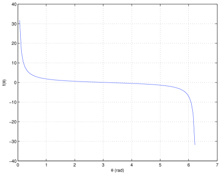
Figure 3: Plot of the function $f(\theta)$.

Furthermore, we will assume without loss of generality that $\theta\in(0,\pi)$ and hence we obtain our first design equation

$$\frac{\sin\theta}{1-\cos\theta}=\frac{|\epsilon|}{\gamma}.$$ (49)

In practice, this ratio would be chosen in the range of $\frac{|\epsilon|}{\gamma}\in(0,0.6)$ in order to ensure that the linearized model which is being used is valid.

Our second design equation is obtained from (48). First we write $C_{p}=\left[\begin{array}[]{ll}C_{p1}&C_{p2}\end{array}\right]$ and define the complex number $c=C_{p1}+\imath C_{p2}$. The argument of this complex number $\arg(c)$ determines the quadrature of interest in the plant. It is straight forward to verify that the condition (48) will be satisfied for some non-zero vector $\beta$ if and only if

$$\arg\left(\imath(\epsilon-\alpha^{*})\right)=\arg(c).$$

That is,

$$\arg\left(\epsilon-\frac{\gamma e^{-\imath\phi}\sin\theta}{1-\cos\theta}\right)=\arg(c)-\frac{\pi}{2}.$$

This is equivalent to

$$\arg\left(\frac{\epsilon}{\gamma}-\frac{e^{-\imath\phi}\sin\theta}{1-\cos\theta}\right)=\arg(c)-\frac{\pi}{2}.$$ (50)

Then we write $\epsilon=|\epsilon|e^{\imath\psi}$. It follows from (49) that (50) can be re-written as

$$\arg\left(e^{\imath\psi}-e^{-\imath\phi}\right)=\arg(c)-\frac{\pi}{2}.$$ (51)

This is our second design equation.

If the design equations (49) and (51) are satisfied then there will exist a non-zero vector $\beta$ such that (48) will be satisfied. Then, we can always find a non-zero vector $C_{o}$ such that (10) is satisfied. Thus, using Theorem 1 we can conclude that if the the design equations (49), (51) are satisfied then the corresponding direct coupled observer will have the desired properties. However, since the proposed experimental implementation of the plant-observer system is a closed quantum system, there is no measurement which can be made on the system to verify the performance of this system. Future research will be directed towards extending the theory developed in [4] to allow for open quantum systems in which a measurement can be made to verify the behaviour of the direct coupled quantum observer.

Example

We now illustrate the above design principles with an example corresponding to typical laboratory values. In this example, we let $C_{p}=\left[\begin{array}[]{ll}1&0\end{array}\right]$ corresponds to the case in which the position quadrature of the plant is of interest. Also, we choose $\gamma=10^{8}$ rad/s and $\omega_{o}=10^{8}$ rad/s. In addition, we choose

$$\frac{|\epsilon|}{\gamma}=0.1$$

which according to (49) corresponds to a value of $\theta=168.6^{\circ}$.

In this case $c=1$ which is purely real and the condition (51) reduces to

$$\arg\left(e^{\imath\psi}-e^{-\imath\phi}\right)=-\frac{\pi}{2}.$$

That is

$$\cos(\psi)-\cos(\phi)=0$$

and

$$\sin(\psi)+\sin(\phi)<0.$$

To satisfy these conditions, we choose $\psi=\phi=-90^{\circ}$. Then, we obtain

$$\epsilon=10^{7}e^{-\imath\frac{\pi}{2}}=-\imath 10^{7}$$

and

$$\alpha=10^{7}e^{-\imath\frac{\pi}{2}}=-\imath 10^{7}.$$

Then, it follows from (48) that

$$\left[\begin{array}[]{ll}2\times 10^{7}&0\\ 0&0\end{array}\right]=\left[\begin{array}[]{l}1\\ 0\end{array}\right]\beta.$$

Hence

$$\beta=\left[\begin{array}[]{ll}2\times 10^{7}&0\end{array}\right].$$

Therefore, if we choose $C_{o}=\left[\begin{array}[]{ll}-10&0\end{array}\right]$, it follows that the condition (10) will be satisfied. Thus, with these parameter values, the proposed implementation will satisfy the conditions of Theorem 1 for a direct coupled quantum observer.

V Conclusion

We have shown that the direct coupling quantum observer proposed in [4] could be at least in theory implemented experimentally. However, such an experiment could not provide experimental verification that the properties of such a quantum observer described in Theorem 1 are satisfied. In order to address this issue, future research will extend the results of [4] to allow for a small probe field. Then the theory developed in this paper will be extended to allow for this case.

Another area of possible future research would be to analyse the performance of the proposed implementation of the plant-observer system without making a linearization assumption in the model of the NDPA.

References

• [1] Z. Miao and M. R. James, “Quantum observer for linear quantum stochastic systems,” in Proceedings of the 51st IEEE Conference on Decision and Control, Maui, December 2012.
• [2] I. Vladimirov and I. R. Petersen, “Coherent quantum filtering for physically realizable linear quantum plants,” in Proceedings of the 2013 European Control Conference, Zurich, Switzerland, July 2013, arXiv:1301.3154.
• [3] Z. Miao, L. A. D. Espinosa, I. R. Petersen, V. Ugrinovskii, and M. R. James, “Coherent quantum observers for finite level quantum systems,” in Australian Control Conference, Perth, Australia, November 2013.
• [4] I. R. Petersen, “A direct coupling coherent quantum observer,” in Proceedings of the 2014 IEEE Multi-conference on Systems and Control, Antibes, France, October 2014, also available arXiv 1408.0399.
• [5] ——, “A direct coupling coherent quantum observer for a single qubit finite level quantum system,” in Proceedings of 2014 Australian Control Conference, Canberra, Australia, November 2014, also arXiv 1409.2594.
• [6] ——, “Time averaged consensus in a direct coupled distributed coherent quantum observer,” in Proceedings of the 2015 American Control Conference, Chicago, IL, July 2015, to appear, accepted 18 Jan 2015.
• [7] ——, “Time averaged consensus in a direct coupled coherent quantum observer network for a single qubit finite level quantum system,” in Proceedings of the 10th ASIAN CONTROL CONFERENCE 2015, Kota Kinabalu, Malaysia, May 2015.
• [8] M. R. James, H. I. Nurdin, and I. R. Petersen, “${H}^{\infty}$ control of linear quantum stochastic systems,” IEEE Transactions on Automatic Control, vol. 53, no. 8, pp. 1787–1803, 2008, arXiv:quant-ph/0703150.
• [9] H. I. Nurdin, M. R. James, and I. R. Petersen, “Coherent quantum LQG control,” Automatica, vol. 45, no. 8, pp. 1837–1846, 2009, arXiv:0711.2551.
• [10] A. J. Shaiju and I. R. Petersen, “A frequency domain condition for the physical realizability of linear quantum systems,” IEEE Transactions on Automatic Control, vol. 57, no. 8, pp. 2033 – 2044, 2012.
• [11] C. Gardiner and P. Zoller, Quantum Noise.   Berlin: Springer, 2000.
• [12] H. Bachor and T. Ralph, A Guide to Experiments in Quantum Optics, 2nd ed.   Weinheim, Germany: Wiley-VCH, 2004.
• [13] A. I. Maalouf and I. R. Petersen, “Bounded real properties for a class of linear complex quantum systems,” IEEE Transactions on Automatic Control, vol. 56, no. 4, pp. 786 – 801, 2011.
• [14] H. Mabuchi, “Coherent-feedback quantum control with a dynamic compensator,” Physical Review A, vol. 78, p. 032323, 2008.
• [15] G. Zhang and M. James, “Direct and indirect couplings in coherent feedback control of linear quantum systems,” IEEE Transactions on Automatic Control, vol. 56, no. 7, pp. 1535–1550, 2011.
• [16] I. G. Vladimirov and I. R. Petersen, “A quasi-separation principle and Newton-like scheme for coherent quantum LQG control,” Systems & Control Letters, vol. 62, no. 7, pp. 550–559, 2013, arXiv:1010.3125.
• [17] I. Vladimirov and I. R. Petersen, “A dynamic programming approach to finite-horizon coherent quantum LQG control,” in Proceedings of the 2011 Australian Control Conference, Melbourne, November 2011, arXiv:1105.1574.
• [18] R. Hamerly and H. Mabuchi, “Advantages of coherent feedback for cooling quantum oscillators,” Physical Review Letters, vol. 109, p. 173602, 2012.
• [19] J. Gough and M. R. James, “The series product and its application to quantum feedforward and feedback networks,” IEEE Transactions on Automatic Control, vol. 54, no. 11, pp. 2530–2544, 2009.
• [20] L. Mandel and E. Wolf, Optical Coherence and Quantum Optics.   Cambridge, UK: Cambridge University Press, 1995.