A Turning Band Approach to
Kernel Convolution for Arbitrary Surfaces

Abstract

One of the most efficient ways to produce unconditional simulations is with the spectral method using fast Fourier transform (FFT) [1]. But this approach is not applicable to arbitrary surfaces because no regular grid exists. However, points on the arbitrary surface can be generated randomly using uniform distribution to replace a regular grid. This paper will describe a nonstationary kernel convolution approach for data on arbitrary surfaces.

I Introduction

The approach to producing unconditional simulations for arbitrary surfaces (sphere, ellipsoid, geoid, torus, etc.) will be described in this paper. The approach is also applicable to nonsmooth surfaces. This paper is based on ideas from a turning band approach ([2], [3], [4], and [5]) and kernel convolution ([6], [7], and [1]). Similar to the turning band, all processing is done on a set of random lines. The difference is in using a random set of points covering an area of interest and projecting them onto the set of random lines. For example, the set of uniformly distributed points on the surface of a sphere is projected onto the set of random lines. The kernel convolution is applied to each line, and the reconstruction of the process is performed similarly to the turning band approach. Using different kernels will produce a nonstationary solution.

II Kernel Convolution by Turning Band

Here are the steps of the algorithm:

1. From a uniform distribution, simulate $\displaystyle N$ points $\displaystyle\vec{s_{i}}$ on a surface.

2. From a standard normal distribution, simulate value $\displaystyle\xi_{i}$ for each point.

3. Simulate $\displaystyle N_{d}$ random or pseudorandom directions (the algorithm to simulate pseudorandom directions can be found in [8] and [5]).

4. Cycle over all directions.

   1. Project points to a direction.

   2. Apply kernel convolution (this is usually done using FFT).

5. For each location where the result is desired, project that location to all directions and average the results of kernel convolutions.

The applied one-dimensional kernel $\displaystyle k_{1}{\left(\bullet\right)}$ will correspond to a three-dimensional kernel $\displaystyle k_{3}{\left(\bullet\right)}$ through integral

$$k_{3}{\left(\vec{h}\right)}=\oiint{k_{1}{\left(\left(\vec{h},\hat{n}\right)\right)}\operatorname{d\!}{\hat{n}}},$$ (1)

where $\displaystyle\left(\vec{x},\vec{y}\right)$ is a scalar product.

The kernel distance is the direct distance in three-dimensional space.

This is similar to the turning band method, and the relationship between three-dimensional or two-dimensional covariance with one-dimensional covariance can be found in [2], [3], and [4]. The same relationship holds true for the kernel functions. In a three-dimensional case, the formula is

$$k_{1}(h)=(h\cdot k_{3}{\left(h\right)})^{\prime}.$$ (2)

In two dimensions for kernel $\displaystyle k_{2}{\left(\bullet\right)}$

$$k_{1}(h)=k_{2}{\left(0\right)}+h\int\limits_{0}^{h}{\dfrac{k_{2}^{\prime}{\left(x\right)}}{\left(h^{2}-x^{2}\right)^{\frac{1}{2}}}\operatorname{d\!}{x}}=k_{2}{\left(0\right)}+h\int\limits_{0}^{\frac{\pi}{2}}{k_{2}^{\prime}{\left(h\sin{\left(\Theta\right)}\right)}\operatorname{d\!}{\Theta}}.$$

III Kernel Convolution for Unconditional Simulation

Applying the algorithm from the section “ Kernel Convolution by Turning Band ” for any location $\displaystyle\vec{s}$ will produce a random field approximately equal to

$$\sum_{i=0}^{N}{\left(k_{3}{\left(\vec{s_{i}}-\vec{s}\right)}\cdot\xi_{i}\right)}.$$ (3)

The approximation is due to the finite number of directions.

The variance at location $\displaystyle\vec{s}$ is approximately equal to

$$\sum_{i=0}^{N}{k_{3}^{2}{\left(\vec{s_{i}}-\vec{s}\right)}}.$$ (4)

For the sphere, the estimate of (4) does not depend on location $\displaystyle\vec{s}$. This does not hold true for other surfaces. However, for any surface with finite sampling $\displaystyle N$, it is not a constant. Calculating this value is important in standardizing unconditional simulations. The estimate of (4) can be found by applying the algorithm from the section “ Kernel Convolution by Turning Band ” for the square of the kernel for the same set of points with values of one. Dividing the approximation of (3) by the square root of the approximation of (4) will produce an approximation of the Gaussian process with unit variance.

Another way to estimate (4) is by producing many unconditional simulations and estimating the variance from them. This will also allow the estimation of covariances.

Compared to the turning band approach, using this algorithm is significantly slower. The slowest part is projecting simulated points to directions. Notice that the simulated points do not depend on the kernel. Therefore, to speed up the approach, it is possible to simulate points and project them to directions in advance. Combining them by bins will significantly reduce the amount of memory necessary to store precalculated results.

IV Conditional Simulations

To perform conditional simulations, it is necessary to know the covariance function. For a sphere, the covariance function is isotropic and does not depend on location. Therefore, it can be derived directly from the kernel as described in [9] and [10]. For arbitrary surfaces, it is possible to make many unconditional simulations and from them estimate the covariance function. Conditional simulations are obtainable from unconditional simulations through solutions of the Kriging system [11], [12], and [13]. [14] describes the approach to construct conditional simulations without abrupt changes.

V Class of Exponential Kernels

Let the kernel function have the form

$$k_{3}{\left(h\right)}=\sum_{i}{\left(P_{i}{\left(h\right)}\cdot\mathsf{e}^{-\Theta_{i}\cdot h}\right)},$$ (5)

where $\displaystyle P_{i}$ is a polynomial.

The result of the convolution can be obtained by the sequential application of the kernel. The technique is described in [15] and [16] with the difference being that the integration is replaced by summation. This reduces the complexity of the kernel convolution from $\displaystyle O{\left(n\cdot\ln{n}\right)}$ to $\displaystyle O{\left(n\right)}$, where $\displaystyle n$ is the number of bins on the line.

For finite kernel

$$k_{3}{\left(h\right)}=\left\{{\begin{aligned} &\sum_{i}{\left(P_{i}{\left(h\right)}\cdot\mathsf{e}^{-\Theta_{i}\cdot h}\right)},&\text{ if }h<T,\\ &0,&\text{ otherwise},\end{aligned}}\right.$$ (6)

where $\displaystyle T$ is the kernel width. To be able to evaluate $\displaystyle k_{1}{\left(h\right)}$ from (2), it is necessary to satisfy $\displaystyle\lim\limits_{h\rightarrow T^{-}}{k_{3}{\left(h\right)}}=0$. Otherwise, $\displaystyle k_{1}{\left(h\right)}$ will not be finite.

There are several advantages of using the finite kernel:

• Ability to produce unconditional simulations for a large area by partitioning it into small pieces (tiles) for independent processing.

• Ability to have a flexible class of kernels in form (6).

The ability to have a flexible class of kernels is important for nonstationary simulations. It allows not only changes in kernel bandwidth but in their shape as well. One way to construct a flexible class of kernels in form (6) is by changing the polynomial part. It is reasonable to use decreasing kernels because the majority of physical processes gradually decreases dependence over distance. From [17], a Bernstein density (a weighted sum of beta probability distribution functions defined on the unit interval $\displaystyle\left[0,1\right]$) is defined as

$$p{\left(x\mid m,\vec{w}\right)}=\sum_{j=1}^{m}\left(\vec{w}_{j}\cdot Beta{\left(x\mid j,m-j+1\right)}\right)\;,\;\vec{w}_{j}\geq 0\;,\;\sum_{j=1}^{m}{\vec{w}_{j}=1}\;,$$

where $\displaystyle m$ is the number of distribution functions, $\displaystyle\vec{w}$ are weights, $\displaystyle Beta{\left(\bullet\right)}$ is the beta probability density function

$$Beta{\left(x\mid j,m-j+1\right)}=\dfrac{m!}{\left(j-1\right)!\cdot\left(m-j\right)!}\cdot x^{j-1}\cdot\left(1-x\right)^{m-j}\;.$$

Forming

$$P{\left(x\right)}=\int\limits_{x}^{1}{p{\left(x\mid m,\vec{w}\right)}}=\sum_{j=1}^{m}\left(\vec{w}_{j}\int\limits_{x}^{1}{Beta{\left(y\mid j,m-j+1\right)}\operatorname{d\!}{y}}\right)$$

and multiplying by $\displaystyle\mathsf{e}^{-\frac{h}{\Theta}}$ produces a flexible family of kernels. The choice of $\displaystyle\Theta$ is arbitrary. If the value is too large, the floating point evaluation will lead to a high round off error. If the value is too small, it will not produce good family of kernels. Let’s define $\displaystyle\Theta=3$.

In the case of $\displaystyle m=2$, this becomes

$$\left\{\begin{aligned} &\left(\vec{w}_{1}\left(1-h\right)^{2}+\vec{w}_{2}\left(1-h^{2}\right)\right)\cdot\mathsf{e}^{-\frac{h}{3}},&\text{ if }h<1,\\ &0,&\text{otherwise},\end{aligned}\right.$$ (7)

where $\displaystyle 0\leq\vec{w}_{i}\leq 1$, $\displaystyle i=1,2$, and $\displaystyle\vec{w}_{1}+\vec{w}_{2}=1$. They are shown in Figure 1a.

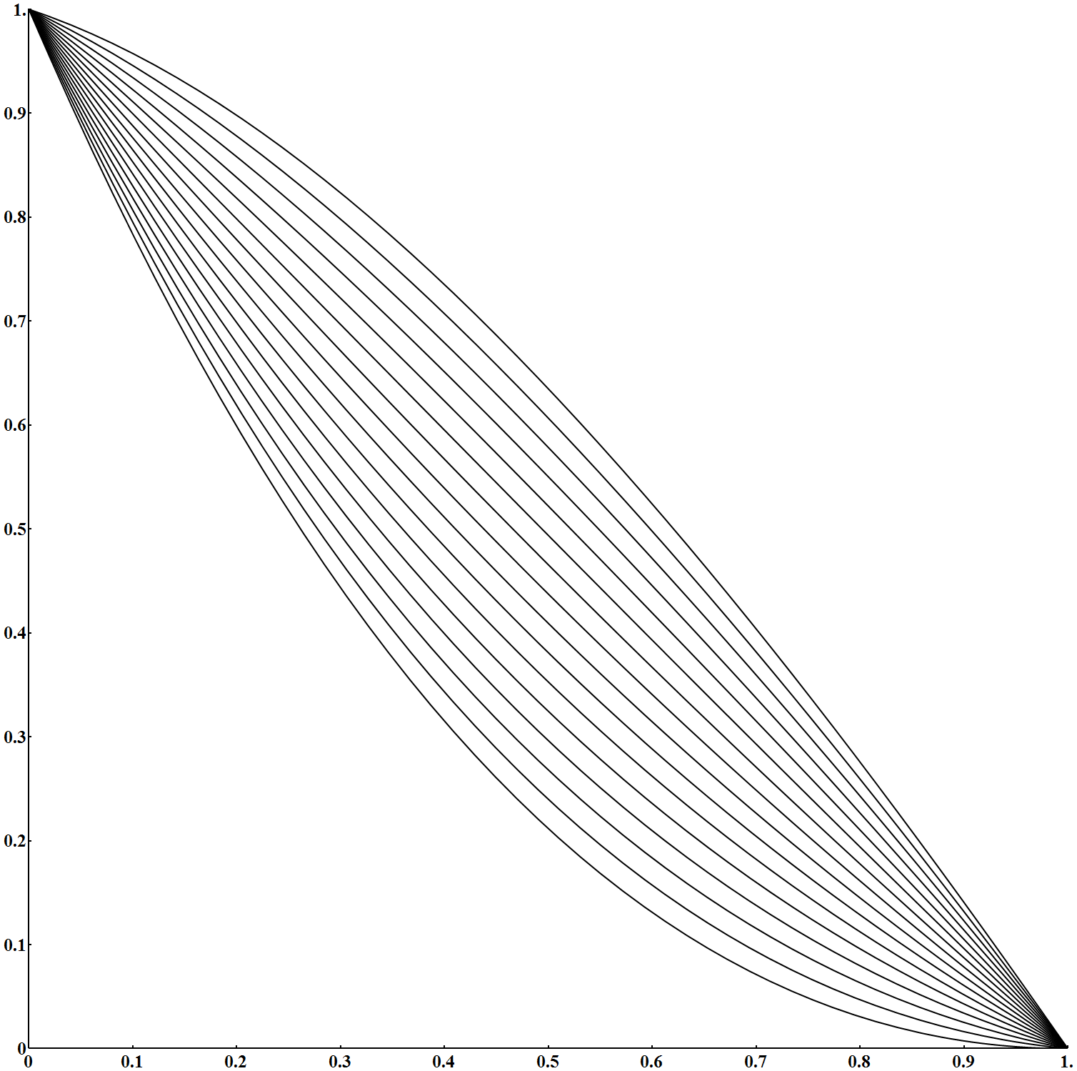
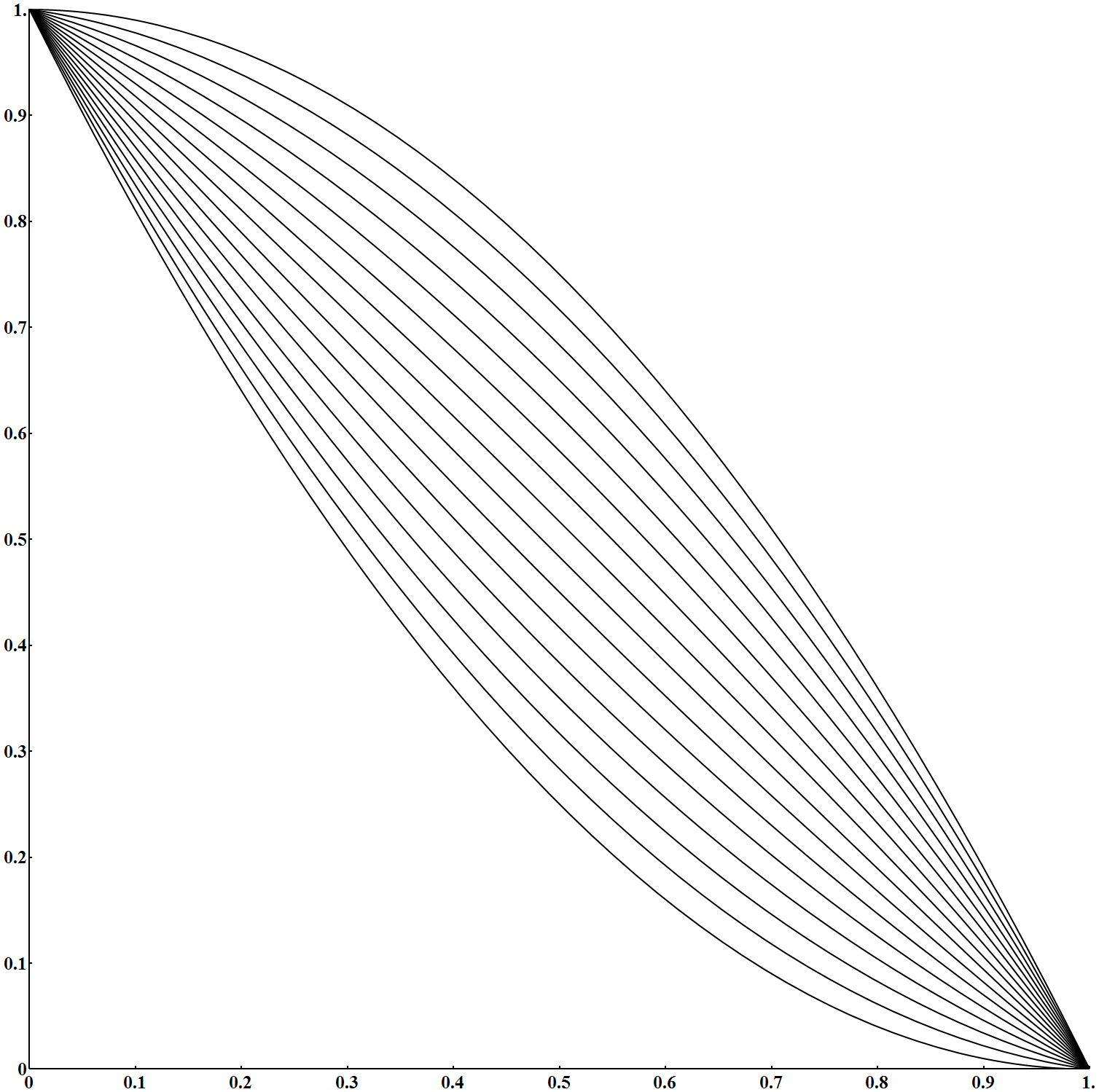
a)	b)

Figure 1: Example of kernels (7). $\displaystyle\vec{w}_{1}=\dfrac{i}{15}$, $\displaystyle\vec{w}_{2}=1-\vec{w}_{1}$, $\displaystyle i=\overline{0..15}$. a) With exponent. b) Without exponent.

In the case of $\displaystyle m=3$

$$\left\{\begin{aligned} &\left(\vec{w}_{1}\left(1-h\right)^{3}+\vec{w}_{2}\left(1-h\right)^{2}\left(1+2h\right)+\vec{w}_{3}\left(1-h^{3}\right)\right)\cdot\mathsf{e}^{-\frac{h}{3}},&\text{ if }h<1,\\ &0,&\text{otherwise},\end{aligned}\right.$$ (8)

where $\displaystyle 0\leq\vec{w}_{i}\leq 1$, $\displaystyle i=1,2,3$, and $\displaystyle\vec{w}_{1}+\vec{w}_{2}+\vec{w}_{3}=1$. They are shown in Figure 2a.

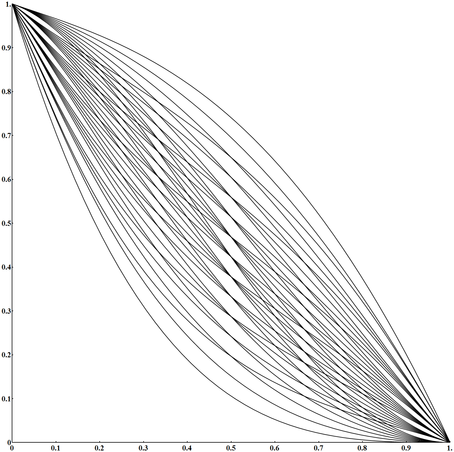
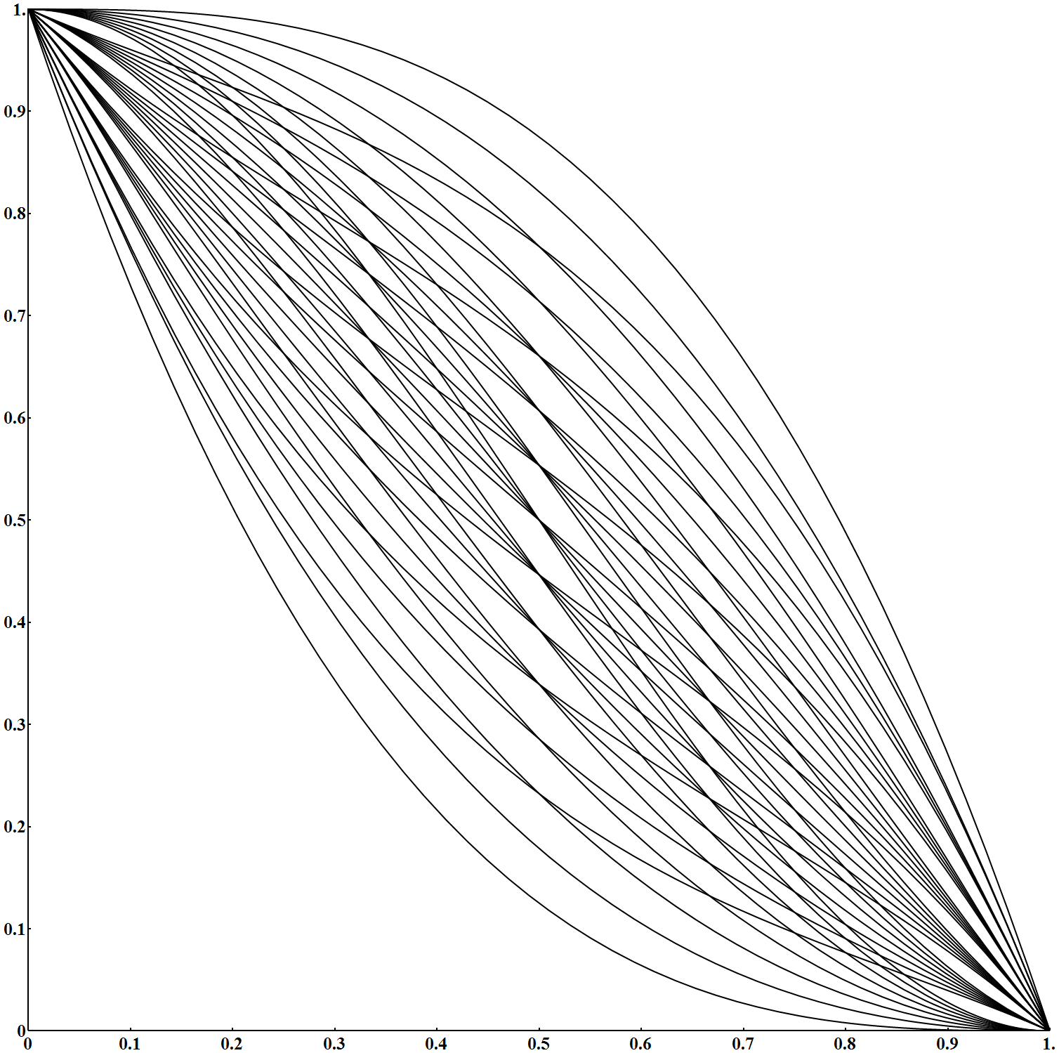
a)	b)

Figure 2: Example of kernels (8). $\displaystyle\vec{w}_{1}=\dfrac{i}{7}$, $\displaystyle\vec{w}_{2}=\dfrac{j}{7}$, $\displaystyle\vec{w}_{3}=1-\vec{w}_{1}-\vec{w}_{2}$, $\displaystyle i=\overline{0..7}$, $\displaystyle j=\overline{0..7-i}$. a) With exponent. b) Without exponent.

From (2), it follows that $\displaystyle k_{1}{\left(h\right)}$ has the same form as (6). Notice that $\displaystyle k_{3}^{2}{\left(h\right)}$ also has the same form, and the one-dimensional kernel corresponding to $\displaystyle k_{3}^{2}{\left(h\right)}$ will be of the same form.

It is possible to extend this approach for anisotropic kernels by adjusting weights and one-dimensional kernel shape in each direction or by stretching the space.

VI Examples

Figure 3 shows unconditional simulation on a torus.

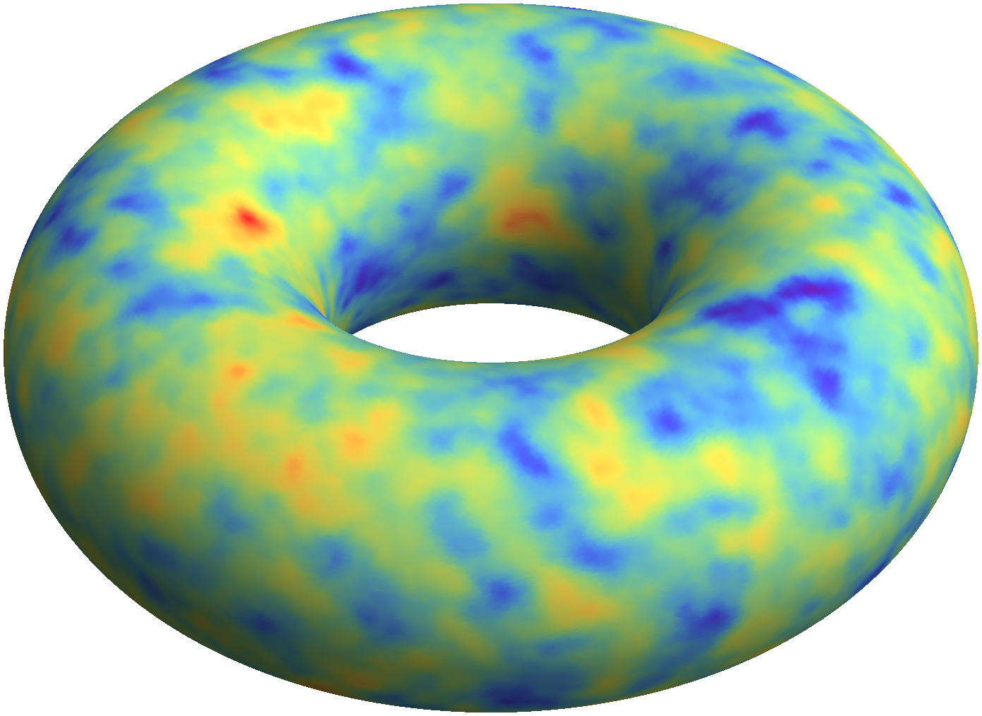
Figure 3: Unconditional simulation on a torus with inner radius 1, outer radius 3, and kernel $\displaystyle\mathsf{e}^{-10h}$. Number of simulated points $\displaystyle N=67,108,864$. Number of random directions $\displaystyle N_{d}=1,024$.

Figure 4 shows nonstationary unconditional simulation on a spheroid with eccentricity equals $\displaystyle\frac{3}{4}$. The kernel changes smoothly in shape from left to right. $\displaystyle 1,024$ unconditional simulations were used to estimate variance and standardize unconditional simulations. Due to changes in the kernel, the right and left parts of the spheroid have different covariance structures. This is visible as a smoother random field on the right compared to the random field on the left.

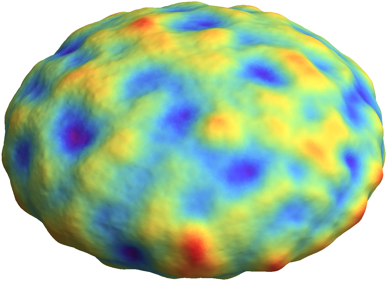
Figure 4: Unconditional simulation on an oblate spheroid with semimajor axis equals $\displaystyle 2$, and semiminor axis equals $\displaystyle 1$. The surface is shown as elevation to depict changes in smoothness. The kernel has the form of (7). It changes smoothly from the kernel on the left $\displaystyle\left(1-\left(3h\right)^{2}\right)\cdot\mathsf{e}^{-h}$ to the kernel on the right $\displaystyle\left(1-3h\right)^{2}\cdot\mathsf{e}^{-h}$ with bandwidth equals $\displaystyle\frac{1}{3}$. Number of simulated points $\displaystyle N=262,144$. Number of random directions $\displaystyle N_{d}=1,024$.

VII Convergence Issue

When the kernel bandwidth tends to be small, the convergence of (3) to the true kernel (1) becomes slow. The number of required directions makes this method inefficient. This is because the distribution of the number of points that are farther away from the center of the kernel (location $\displaystyle\vec{s}$ in (3)) in three dimensions increases squarely. This is even true for some directions when points are only located on the surface.

VIII Tile Approach

Finite kernel and overlapping tiles overcome the issue described in the previous section. For example, in two dimensions, if all tiles are $\displaystyle 2$ by $\displaystyle 2$ and start from integer numbers (corners can be rounded), then the kernel with a bandwidth not exceeding $\displaystyle\frac{1}{2}$ will always be completely inside at least one tile; see Figure 5. This is applicable in any number of dimensions.

Figure 5: The red circle is the area covered by a finite kernel. The blue rounded square is the tile completely covering the finite kernel.

The bandwidth should not be significantly smaller than the tile width, and the exponential part in the kernel can be dropped. The flexible family of kernels without the exponential part is shown in Figures 1b and 2b.

Figure 6a shows the effect of using the tile approach. The small discontinuities are visible in the horizontal and vertical lines passing through the center. Increasing the number of bands will reduce this effect. Figure 6b shows the result of evaluating (3) and (4) directly.

a)	b)

Figure 6: Unconditional simulation in two dimensions by kernel $\displaystyle k_{3}{\left(h\right)}=\left(1-2h\right)^{2}$ with bandwidth equals $\displaystyle\frac{1}{2}$. Number of simulated points $\displaystyle N=65,536$. a) The tile approach with the number of random directions $\displaystyle N_{d}=1,024$ (uniformly distributed in three dimensions). b) Direct calculation.

If a continuous result is required, overlapped tiles can be joined smoothly. This will increase calculations by the number of tiles necessary to process. One way to reduce the number of tiles is to use a triangular grid (use nonequilateral triangles for arbitrary surfaces). For each node of the triangular grid, define a tile that covers all neighboring triangles and at least a kernel bandwidth. For each triangle, the barycentric coordinate system will give weights for the tiles. There will only be a maximum of three tiles with nonzero weights; therefore, the complexity is increased three times.

IX Using Integer Arithmetic

In the turning band approach, the directions are chosen randomly or pseudorandomly. In this section, another approach will be described to make directions proportional to integer numbers. Using such directions will remove errors from applying fixed steps (bins) in each direction.

Let’s take a sphere of radius $\displaystyle R=\sqrt{S}$, where $\displaystyle S$ is a natural number. If the radius $\displaystyle R$ approaches infinity, all integer vectors inside the sphere (all integer vertices except the center of a coordinate system) tend to be uniformly distributed. However, the unique directions are not uniformly distributed (see example in Figure 7a). But assigning a proper weight to each direction will resolve it. The appropriate weights can be assigned as proportionate to the number of vectors with the same direction or to the area of the spherical Voronoi diagram cells.

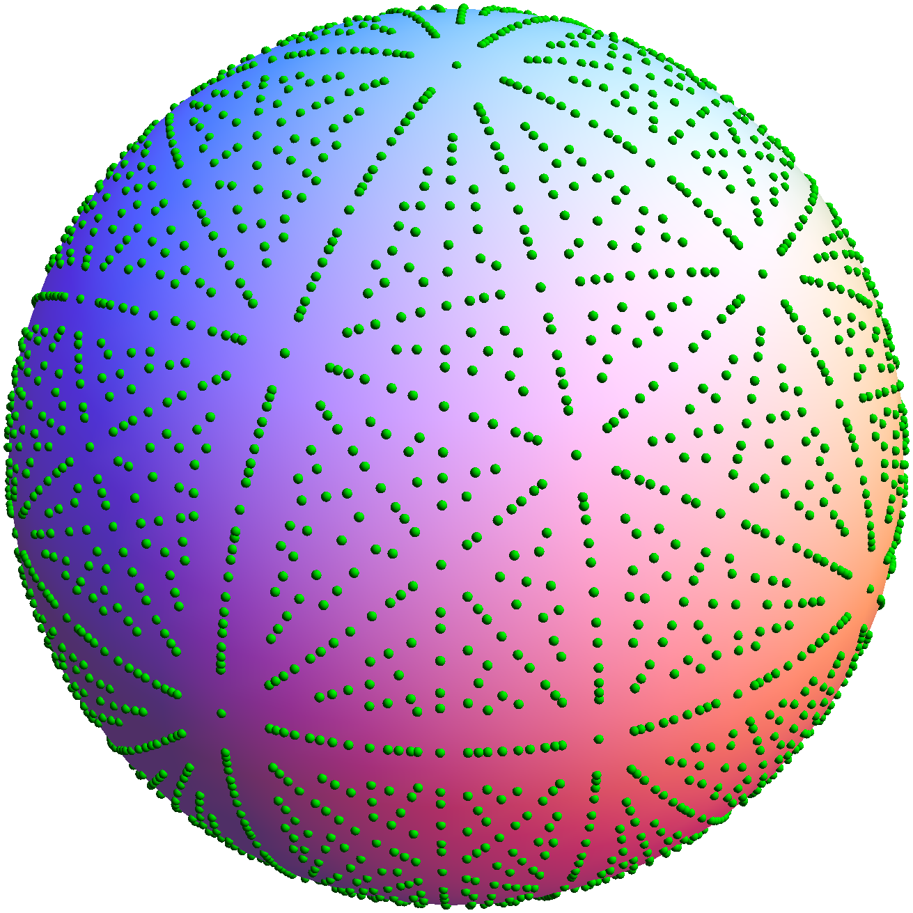
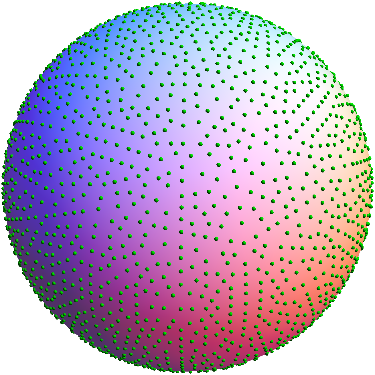
a)	b)

Figure 7: a) All integer directions are shown as dots on the sphere for $\displaystyle S=100$. The number of unique directions equals $\displaystyle 1,729$ (counting $\displaystyle\vec{v}$ and $\displaystyle-\vec{v}$ once). b) A uniform set of integer directions satisfying that any two directions are at least $\displaystyle 3\degree$ apart. The number of directions equals $\displaystyle 1,405$.

Selecting only directions separated by some degree will make a uniform coverage (see Figure 7b). The list of integer directions is shown in the appendix. This is similar to using a set of pseudorandom directions as described in [8] and [5].

Because each direction is represented as $\displaystyle\alpha\cdot\left(x,y,z\right)$, where $\displaystyle\alpha$ is a real number (square root of a natural number) and $\displaystyle x$, $\displaystyle y$, and $\displaystyle z$ are integers, any coordinate with integer components will be projected to a position $\displaystyle\alpha\cdot i$, where $\displaystyle i$ is an integer number.

If random points are placed on an integer grid, there are no errors due to binning. If the resultant location also has an integer coordinate, there is no additional error. Notice that the kernel (5) or (6) can be calculated for any position on direction, see [15] and [16]. The turning band approach [2], [3], [4], and [5] might also benefit from using integer arithmetic.

X Conclusion

The new approach to producing unconditional nonstationary simulations on arbitrary surfaces is equivalent to the kernel convolution approach with the kernel shape depending on location ([6], [7], and [1]). Applying a kernel to the arbitrary surfaces produces a larger class of valid covariance functions than the class of valid covariance functions in three-dimensional space.

Precalculating projections of random points in all directions for all tiles might be necessary for the efficiency of the approach. Nevertheless, even with precalculations, this approach is not efficient. The better approach is based on kernel convolution using FFT as described in [18].

New flexible classes of kernels constructed from polynomials are described in this paper. Because they are linear combinations of some basis kernels, constructing covariances for all pairs of basis kernels is sufficient to calculate covariance between any two kernels. Unconditional simulation for a nonstationary kernel is a weighted sum of unconditional simulations corresponding to basis kernels for the same set of random points.

Using integer arithmetic, an error introduced in the turning band approach due to binning along each direction can be avoided.

XI Acknowledgment

The author would like to thank David Burrows for help with area preserving transformation from authalic sphere to spheroid (authalic sphere is a sphere were the surface area equals the spheroid surface area). This transformation was used in simulating uniformly distributed random points on the surface of a spheroid for the creation of Figure 4.

Appendix. List of Integer Directions

Integer directions that are at least $\displaystyle 3\degree$ apart: $\displaystyle\left(1,0,0\right)$, $\displaystyle\frac{\left(1,1,0\right)}{\sqrt{2}}$, $\displaystyle\frac{\left(1,1,1\right)}{\sqrt{3}}$, $\displaystyle\frac{\left(2,1,0\right)}{\sqrt{5}}$, $\displaystyle\frac{\left(2,1,1\right)}{\sqrt{6}}$, $\displaystyle\frac{\left(3,1,0\right)}{\sqrt{10}}$, $\displaystyle\frac{\left(2,2,1\right)}{3}$, $\displaystyle\frac{\left(3,1,1\right)}{\sqrt{11}}$, $\displaystyle\frac{\left(3,2,0\right)}{\sqrt{13}}$, $\displaystyle\frac{\left(4,1,0\right)}{\sqrt{17}}$, $\displaystyle\frac{\left(3,2,1\right)}{\sqrt{14}}$, $\displaystyle\frac{\left(4,1,1\right)}{\sqrt{18}}$, $\displaystyle\frac{\left(3,2,2\right)}{\sqrt{17}}$, $\displaystyle\frac{\left(3,3,1\right)}{\sqrt{19}}$, $\displaystyle\frac{\left(4,2,1\right)}{\sqrt{21}}$, $\displaystyle\frac{\left(4,3,0\right)}{5}$, $\displaystyle\frac{\left(5,1,1\right)}{\sqrt{27}}$, $\displaystyle\frac{\left(5,2,0\right)}{\sqrt{29}}$, $\displaystyle\frac{\left(6,1,0\right)}{\sqrt{37}}$, $\displaystyle\frac{\left(3,3,2\right)}{\sqrt{22}}$, $\displaystyle\frac{\left(4,3,1\right)}{\sqrt{26}}$, $\displaystyle\frac{\left(5,2,1\right)}{\sqrt{30}}$, $\displaystyle\frac{\left(4,3,2\right)}{\sqrt{29}}$, $\displaystyle\frac{\left(4,4,1\right)}{\sqrt{33}}$, $\displaystyle\frac{\left(5,2,2\right)}{\sqrt{33}}$, $\displaystyle\frac{\left(5,3,1\right)}{\sqrt{35}}$, $\displaystyle\frac{\left(6,2,1\right)}{\sqrt{41}}$, $\displaystyle\frac{\left(7,1,1\right)}{\sqrt{51}}$, $\displaystyle\frac{\left(4,3,3\right)}{\sqrt{34}}$, $\displaystyle\frac{\left(5,3,2\right)}{\sqrt{38}}$, $\displaystyle\frac{\left(5,4,1\right)}{\sqrt{42}}$, $\displaystyle\frac{\left(6,3,1\right)}{\sqrt{46}}$, $\displaystyle\frac{\left(9,1,0\right)}{\sqrt{82}}$, $\displaystyle\frac{\left(5,4,2\right)}{\sqrt{45}}$, $\displaystyle\frac{\left(6,3,2\right)}{7}$, $\displaystyle\frac{\left(6,4,1\right)}{\sqrt{53}}$, $\displaystyle\frac{\left(7,3,1\right)}{\sqrt{59}}$, $\displaystyle\frac{\left(7,4,0\right)}{\sqrt{65}}$, $\displaystyle\frac{\left(8,2,1\right)}{\sqrt{69}}$, $\displaystyle\frac{\left(5,4,3\right)}{\sqrt{50}}$, $\displaystyle\frac{\left(7,3,2\right)}{\sqrt{62}}$, $\displaystyle\frac{\left(10,1,1\right)}{\sqrt{102}}$, $\displaystyle\frac{\left(6,4,3\right)}{\sqrt{61}}$, $\displaystyle\frac{\left(6,5,2\right)}{\sqrt{65}}$, $\displaystyle\frac{\left(6,6,1\right)}{\sqrt{73}}$, $\displaystyle\frac{\left(7,4,2\right)}{\sqrt{69}}$, $\displaystyle\frac{\left(7,6,0\right)}{\sqrt{85}}$, $\displaystyle\frac{\left(10,2,1\right)}{\sqrt{105}}$, $\displaystyle\frac{\left(5,5,4\right)}{\sqrt{66}}$, $\displaystyle\frac{\left(7,6,1\right)}{\sqrt{86}}$, $\displaystyle\frac{\left(10,3,1\right)}{\sqrt{110}}$, $\displaystyle\frac{\left(7,4,4\right)}{9}$, $\displaystyle\frac{\left(8,6,1\right)}{\sqrt{101}}$, $\displaystyle\frac{\left(9,5,1\right)}{\sqrt{107}}$, $\displaystyle\frac{\left(11,3,2\right)}{\sqrt{134}}$, $\displaystyle\frac{\left(11,4,1\right)}{\sqrt{138}}$, $\displaystyle\frac{\left(8,7,2\right)}{\sqrt{117}}$, $\displaystyle\frac{\left(11,5,1\right)}{\sqrt{147}}$, $\displaystyle\frac{\left(7,6,5\right)}{\sqrt{110}}$, $\displaystyle\frac{\left(11,4,3\right)}{\sqrt{146}}$, $\displaystyle\frac{\left(7,6,6\right)}{11}$, $\displaystyle\frac{\left(8,7,4\right)}{\sqrt{129}}$, $\displaystyle\frac{\left(10,5,4\right)}{\sqrt{141}}$, $\displaystyle\frac{\left(11,7,1\right)}{\sqrt{171}}$, $\displaystyle\frac{\left(17,1,1\right)}{\sqrt{291}}$, $\displaystyle\frac{\left(18,1,0\right)}{\sqrt{325}}$, $\displaystyle\frac{\left(13,4,3\right)}{\sqrt{194}}$, $\displaystyle\frac{\left(16,4,1\right)}{\sqrt{273}}$, $\displaystyle\frac{\left(18,3,1\right)}{\sqrt{334}}$, $\displaystyle\frac{\left(10,7,6\right)}{\sqrt{185}}$, $\displaystyle\frac{\left(10,9,4\right)}{\sqrt{197}}$, $\displaystyle\frac{\left(11,11,1\right)}{\sqrt{243}}$, $\displaystyle\frac{\left(12,8,3\right)}{\sqrt{217}}$, $\displaystyle\frac{\left(12,7,6\right)}{\sqrt{229}}$, $\displaystyle\frac{\left(14,12,1\right)}{\sqrt{341}}$, and $\displaystyle\frac{\left(17,12,1\right)}{\sqrt{434}}$. The complete list of directions is formed by considering for each vector all signs and permutations of its components.

References

- [1] J. M. Ver Hoef, N. Cressie, and R. P. Barry, “Flexible spatial models for kriging and cokriging using moving averages and the fast Fourier transform (FFT),” Journal of Computational and Graphical Statistics, vol. 13, no. 2, pp. 265–282, 2004. [Online]. Available: http://www.jstor.org/stable/1391176
- [2] P. I. Brooker, “Two-dimensional simulation by turning bands,” Journal of the International Association for Mathematical Geology, vol. 17, no. 1, pp. 81–90, 1985. [Online]. Available: http://doi.org/10.1007/BF01030369
- [3] C. R. Dietrich, “A simple and efficient space domain implementation of the turning bands method,” Water Resources Research, vol. 31, no. 1, pp. 147–156, 1995. [Online]. Available: http://doi.org/10.1029/94WR01457
- [4] T. Gneiting, “Closed form solutions of the two-dimensional turning bands equation,” Mathematical Geology, vol. 30, no. 4, pp. 379–390, 1998. [Online]. Available: http://doi.org/10.1023/A%3A1021792107170
- [5] X. Emery and C. Lantuéjoul, “Tbsim: A computer program for conditional simulation of three-dimensional Gaussian random fields via the turning bands method,” Computers & Geosciences, vol. 32, no. 10, pp. 1615–1628, 2006. [Online]. Available: http://doi.org/10.1016/j.cageo.2006.03.001
- [6] R. P. Barry and J. M. Ver Hoef, “Blackbox kriging: Spatial prediction without specifying variogram models,” Journal of Agricultural, Biological, and Environmental Statistics, vol. 1, no. 3, pp. 297–322, September 1996. [Online]. Available: http://www.jstor.org/stable/1400521
- [7] D. Higdon, “A process-convolution approach to modelling temperatures in the North Atlantic ocean,” Environmental and Ecological Statistics, vol. 5, no. 2, pp. 173–190, 1998. [Online]. Available: http://dx.doi.org/10.1023/A%3A1009666805688
- [8] X. Freulon and C. de Fouquet, “Remarques sur la pratique des bandes tournantes a 3D,” Cahiers de géostatistique, pp. 101–117, June 1991. [Online]. Available: http://www.cg.ensmp.fr/bibliotheque/public/FREULON_Publication_00508.pdf
- [9] A. Gribov and K. Krivoruchko, “Flexible compact covariance model on a sphere,” in Stochastic Environmental Research and Risk Assessment, 2015, (submitted).
- [10] ——, “Simulations from spatially varying kriging model with compactly supported covariance,” in Proceedings of the 17th annual conference of the International Association for Mathematical Geosciences, IAMG2015, Freiberg, Germany, 2015, (submitted).
- [11] A. G. Journel, “Geostatistics for conditional simulation of ore bodies,” Economic Geology, vol. 69, no. 5, pp. 673–687, 1974. [Online]. Available: http://doi.org/10.2113/gsecongeo.69.5.673
- [12] A. G. Journel and C. J. Huijbregts, Mining Geostatistics. Academic Press Inc., December 1978.
- [13] W. J. K. Aldworth, “Spatial prediction, spatial sampling, and measurement error,” p. 186, 1998, Retrospective Theses and Dissertations. [Online]. Available: http://lib.dr.iastate.edu/rtd/11842
- [14] A. Gribov and K. Krivoruchko, “Geostatistical mapping with continuous moving neighborhood,” Mathematical Geology, vol. 36, no. 2, pp. 267–281, 2004. [Online]. Available: http://doi.org/10.1023/B%3AMATG.0000020473.63408.17
- [15] E. Bodansky, A. Gribov, and M. Pilouk, “Smoothing and compression of lines obtained by raster-to-vector conversion,” in Graphics Recognition Algorithms and Applications, ser. Lecture Notes in Computer Science, D. Blostein and Y.-B. Kwon, Eds. Springer Berlin Heidelberg, 2002, vol. 2390, pp. 256–265. [Online]. Available: http://doi.org/10.1007/3-540-45868-9_22
- [16] A. Gribov and E. Bodansky, “Smoothing a network of planar polygonal lines obtained with vectorization,” in Graphics Recognition. Recent Advances and New Opportunities, ser. Lecture Notes in Computer Science, W. Liu, J. Lladós, and J.-M. Ogier, Eds. Springer Berlin Heidelberg, 2008, vol. 5046, pp. 213–234. [Online]. Available: http://doi.org/10.1007/978-3-540-88188-9_21
- [17] J. T. A. S. Ferreira, F. A. Quintana, and M. F. J. Steel, “Flexible univariate continuous distributions,” Bayesian Analysis, vol. 4, no. 3, pp. 497–521, 2009.
- [18] A. Gribov, “Efficient kernel convolution for smooth surfaces,” 2015, in preparation.