A new method for choosing parameters in delay reconstruction-based forecast strategies

Abstract

Delay-coordinate reconstruction is a proven modeling strategy for building effective forecasts of nonlinear time series. The first step in this process is the estimation of good values for two parameters, the time delay and the embedding dimension. Many heuristics and strategies have been proposed in the literature for estimating these values. Few, if any, of these methods were developed with forecasting in mind, however, and their results are not optimal for that purpose. Even so, these heuristics—intended for other applications—are routinely used when building delay coordinate reconstruction-based forecast models. In this paper, we propose a new strategy for choosing optimal parameter values for forecast methods that are based on delay-coordinate reconstructions. The basic calculation involves maximizing the shared information between each delay vector and the future state of the system. We illustrate the effectiveness of this method on several synthetic and experimental systems, showing that this metric can be calculated quickly and reliably from a relatively short time series, and that it provides a direct indication of how well a near-neighbor based forecasting method will work on a given delay reconstruction of that time series. This allows a practitioner to choose reconstruction parameters that avoid any pathologies, regardless of the underlying mechanism, and maximize the predictive information contained in the reconstruction.

I Introduction

The method of delays is a well-established technique for reconstructing the state-space dynamics of a system from scalar time-series datatakens ; packard80 ; sauer91 . The task of choosing good values for the free parameters in this procedure has been the subject of a large and active body of literature over the past few decades, e.g.,Olbrich97 ; fraser-swinney ; kantz97 ; Buzug92Comp ; liebert-wavering ; Buzugfilldeform ; Liebert89 ; rosenstein94 ; Cao97Embed ; Kugi96 ; KBA92 ; Hegger:1999yq . The majority of these techniques focus on the geometry of the reconstruction. A standard method for selecting the delay $\tau$, for instance, is to maximize independence between the coordinates of the delay vector while minimizing overfolding and reduction in causality between coordinatesfraser-swinney ; a common way to choose an embedding dimension is to track changes in near-neighbor relationships in reconstructions of different dimensionsKBA92 .

This heavy focus on the geometry of the delay reconstruction is appropriate when one is interested in quantities like fractal dimension and Lyapunov exponents, but it is not necessarily the best approach when one is building a delay reconstruction for the purposes of prediction. That issue, which is the focus of this paper, has received comparatively little attention in the extensive literature on delay reconstruction-based predictionweigend-book ; casdagli-eubank92 ; Smith199250 ; pikovsky86-sov ; sugihara90 ; lorenz-analogues . In the following section, we propose a robust, computationally efficient method called SPI that can be used to select parameter values that maximize the shared information between the past and the future—or, equivalently, that maximize the reduction in uncertainty about the future given the current model of the past. The implementation details, and a complexity analysis of the algorithm, are covered in Section III. In Section IV, we show that simple prediction methods working with SPI-optimal reconstructions—constructions using parameter values that follow from the SPI calculations—perform better, on both real and synthetic examples, than those same forecast methods working with reconstructions that are built using the traditional methods mentioned above. Finally, in Section V we explore the utility of SPI in the face of different data lengths and prediction horizons.

II Shared information and delay reconstructions

The information shared between the past and the future is known as the excess entropycrutchfield2003regularities . We will denote it here by $E=I[\overleftarrow{X};\overrightarrow{X}]$, where $I$ is the mutual informationyeung2012first and $\overleftarrow{X}$ and $\overrightarrow{X}$ represent the infinite past and the infinite future, respectively. $E$ is often difficult to estimate from data due to the need to calculate statistics over potentially infinite random variablesjames2014many . While this is possible in principle, it is too difficult in practice for all but the simplest of dynamicsstrelioff2014bayesian . In any case, the excess entropy is not exactly what one needs for the purposes of prediction, since it is not realistic to expect to have the infinite past or to predict infinitely far into the future. For our purposes, it is more productive to consider the information contained in the recent past and determine how much that explains about the not-too-distant future. To that end, we define

$$SPI={I}[\mathcal{S}_{j};X_{j+p}]~{},$$

where $\mathcal{S}_{j}$ is an estimate of the state of the system at time $j$ and $X_{j+p}$ is the state of the system $p$ steps in the future.

This can be neatly visualized—and compared to traditional methods like time-delayed mutual information, multi-information and the so-called co-informationBell03theco-information —using the I-diagrams of Yeungyeung2012first . Figure 1 shows an I-diagram of time-delayed mutual information for a specific $\tau$. In a diagram like this, each circle represents the uncertainty in a particular variable. The left circle in Figure 1, for instance, represents the average uncertainty in observing $X_{j-\tau}$ (i.e., $H[X_{j-\tau}]$, where $H$ is the Shannon entropyyeung2012first ); similarly, the top circle represents $H[X_{j+p}]$ or the uncertainty in the $p^{th}$ future observation. Each of the overlapping regions represents shared uncertainty: e.g., in Figure 1, the shaded region represents the shared uncertainty between $X_{j}$ and $X_{j-\tau}$. More precisely, the shaded region schematizes the quantity

$$I[X_{j};X_{j-\tau}] = H[X_{j}]+H[X_{j-\tau}]-H[X_{j},X_{j-\tau}]$$

$$= H[X_{j}]-H[X_{j}|X_{j-\tau}]$$

$$= H[X_{j-\tau}]-H[X_{j-\tau}|X_{j}].$$

If the $X$ are trajectories in reconstructed state space, then tuning the reconstruction parameters (e.g., $\tau$) changes the size of the overlap regions—i.e., the amount of information shared between the coordinates of the delay vector. This notion can be put into practice to select good values for those parameters. Notice, for instance, that minimizing the shaded region in Figure 1—that is, rendering $X_{j}$ and $X_{j-\tau}$ as independent as possible—maximizes the total uncertainty that is explained by the combined model $[X_{j},X_{j-\tau}]^{T}$ (the sum of the area of the two circles). This is precisely the argument made by Fraser and Swinney in fraser-swinney . However, it is easy to see from the I-diagram that choosing $\tau$ in this way does not explicitly take into account explanations of the future—that is, it does not reduce the uncertainty about $X_{t+p}$. Moreover, the calculation does not extend to three or more variables, where minimizing overlap is not a trivial extension of the reasoning captured in the I-diagrams.

Figure 1: An I-diagram of the time-delayed mutual information. The circles represent uncertainties ($H$) in different variables; the shaded region represents $I[X_{j};X_{j-\tau}]$, the time-delayed mutual information between the current state $X_{j}$ and the state $\tau$ time units in the past, $X_{j-\tau}$. Notice that the shaded region is indifferent to $H[X_{j+p}]$, the uncertainty about the future.

The obvious next step would be to explicitly include the future in the estimation procedure. One approach to this would be to work with the so-called co-informationBell03theco-information ,

$$\mathcal{C}=I[X_{j};X_{j-\tau};X_{j+p}]~{},$$

As depicted in Figure 2(a), this is the intersection of $H[X_{j}]$, $H[X_{j-\tau}]$ and $H[X_{j+p}]$. It describes the reduction in uncertainty that the two past states, together, provide regarding the future. While this is obviously an improvement over the time-delayed mutual information of Figure 1, it does not take into account the information that is shared between $X_{j}$ and the future but not shared with the past (i.e., $X_{j-\tau}$), and vice versa. The so-called multi-information,

$$\mathcal{M}=\sum_{\mathclap{i\in\{j,j-\tau,j+p\}}}\left(H[X_{i}]\right)-H[X_{j},X_{j-\tau},X_{j+p}]~{},$$

depicted in Figure 2(b) addresses this shortcoming, but it also includes information that is shared between the past and the present, but not with the future. This is not terribly useful for the purposes of prediction. Moreover, the multi-information overweights information that is shared between all three circles—past, present, and future—thereby artificially over-valuing information that is shared in all delay coordinates. In the context of predicting $X_{t+p}$, the provenance of the information is irrelevant and so the multi-information seems ill-suited to the task at hand as well.

(a) The co-information, $\mathcal{C}[X_{j+1};X_{j};X_{j-\tau}]$

(b) An I-diagram of the multi-information, $\mathcal{M}[X_{j},X_{j-\tau};X_{j+p}]$. The centermost region is more darkly shaded here to reflect the extra weight that that region carries in the calculation.

SPI addresses all of the issues raised in the previous paragraphs. By treating the generic delay vector as a joint variable, rather than a series of single variables, SPI captures the shared information between the past, present, and future independently (the left and right colored wedges in Figure 3), as well as the information that the past and present, together, share with the future (the center wedge). By choosing delay reconstruction parameters that maximize SPI, then, one can explicitly maximize the amount of information that each delay vector contains about the future.

Figure 3: An I-diagram of SPI, the quantity proposed in this paper: $I[[X_{j},X_{j-\tau}];X_{j+p}]$. This quantity captures the shared information between the past, present, and future independently, as well as the information that the past and present, together, share with the future.

To make all of this more concrete and tie it back to state-space prediction of dynamical systems, consider the following example: let $\mathcal{S}_{j}$ be a two-dimensional delay reconstruction of the time series, $\mathcal{S}_{j}=[x_{j},x_{j-\tau}]^{T}$. In this case, SPI becomes $I[[X_{j},X_{j-\tau}]^{T};X_{t+p}]$, which describes the reduction in uncertainty about the system at time $j+p$, given the state estimate $[X_{j},X_{j-\tau}]^{T}$. One can estimate a $\tau$ value for the purposes of reconstructing the dynamics from a given time series, for instance, by calculating SPI for a range of $\tau$ and choosing the first maximum (i.e., minimizing the uncertainty about the $p^{th}$ future observation). One can then apply any state-space forecasting method to the resulting reconstruction in order to predict the future course of that time series. In Section IV, we explore that claim using Lorenz’s classic method of analogueslorenz-analogues , but it should be just as applicable for other predictors that utilize state-space reconstructions, such as the methods used inweigend-book ; casdagli-eubank92 ; Smith199250 ; sugihara90 .

Notice that both the definition of SPI and its use in optimizing forecast algorithms are general ideas that are easily extensible to other state estimators. For example, in the case of traditional delay-coordinate embedding, the state estimator is the $m$-dimensional delay vector, i.e.,

$$\mathcal{S}_{j}=[X_{j},X_{j-\tau},\dots,X_{j-(m-1)\tau)}]^{T}$$

with $m$ chosen to meet the appropriate theoretical requirements takens ; sauer91 . We demonstrate this approach in Section IV. If the time series is pre-processed (e.g., via a Kalman filtersorenson , a low-pass filter and an inverse Fourier transformsauer-delay , or some other local linear transformationweigend-book ; casdagli-eubank92 ; Smith199250 ; sugihara90 ; kantz97 ), the state estimator simply becomes $\mathcal{S}_{j}=\hat{\vec{x}}_{j}$ where $\hat{\vec{x}}_{j}$ is the processed $m$-dimensional delay vector. As we demonstrate in Section IV.2.2, one can even use SPI to optimize parameter choices for forecast methods that use reconstructions that are not embeddings—i.e., those whose dimensions do not meet the traditional requirements for preserving dynamical invariants like the Lyapunov exponent.

III Efficient estimation of SPI

To calculate SPI from a real-valued time series, one must first symbolize those data. Simple binning is not a good solution here, as it is known to cause severe bias if the bin boundaries do not create a generating partitionKSG . A useful alternative is kernel estimation PhysRevLett.85.461 ; PhysRevLett.99.204101 , in which the relevant probability density functions are estimated via a function $\Theta$ with a resolution or bandwidth $r$ that measures the similarity between two points in $X\times Y$ space. (For SPI, $X$ would be $\mathcal{S}_{j}$ and $Y$ would be $X_{j+p}$.) Given points $\{x_{i},y_{i}\}$ and $\{x^{\prime}_{i},y^{\prime}_{i}\}$ in $X\times Y$, one can define:

$$\hat{p}_{r}(x_{i},y_{i})=\frac{1}{N}\sum_{i^{\prime}=1}^{N}\Theta\left(\begin{array}[]{|c|}x_{i}-x^{\prime}_{i}\\ y_{i}-y^{\prime}_{i}\end{array}-r\right)~{},$$

where $\Theta(x>0)=0$ and $\Theta(x\leq 0)=1$. That is, $\hat{p}_{r}(x_{i},y_{i})$ is the proportion of the $N$ pairs of points in $X\times Y$ space that fall within the kernel bandwidth $r$ of $\{x_{i},y_{i}\}$, i.e., the proportion of points similar to $\{x_{i},y_{i}\}$. When $|\cdot|$ is the max norm, this is the so-called box kernel. This too, however, can introduce biasjidt and is dependent on the choice of bandwidth $r$. After these estimates, and the analogous estimates for $\hat{p}(x)$, are produced, they are then used directly to compute local estimates of mutual information for each point in space, which are then averaged over all samples to produce the mutual information of the time series. For more details on this procedure, seejidt .

A better way to calculate $I[X;Y]$ and estimate SPI is the Kraskov-Stügbauer-Grassberger (KSG) estimatorKSG . This approach dynamically alters the kernel bandwidth to match the density of the data, thereby smoothing out errors in the probability density function estimation process. In this approach, one first finds the $k^{th}$ nearest neighbor for each sample $\{x,y\}$ (using max norms to compute distances in $x$ and $y$), then sets kernel widths $r_{x}$ and $r_{y}$ accordingly and performs the pdf estimation. There are two algorithms for computing $I[X;Y]$ with the KSG estimatorjidt . The first is more accurate for small sample sizes but more biased; the second is more accurate for larger sample sizes. We use the second of the two in this paper, as we have fairly long time series. Our algorithm sets $r_{x}$ and $r_{y}$ to the $x$ and $y$ distances to the $k^{th}$ nearest neighbor. One then counts the number of neighbors within and on the boundaries of these kernels in each marginal space, calling these sums $n_{x}$ and $n_{y}$, and finally calculates

$$I[X;Y]=\psi(k)-\frac{1}{k}-\langle\psi(n_{x})+\psi(n_{y})\rangle+\psi(n)~{},$$

where $\psi$ is the digamma function. This estimator has been demonstrated to be robust to variations in $k$ as long as $k\geq 4$jidt .

In this paper, we employ the Java Information Dynamics Toolkit (JIDT) implementation of the KSG estimatorjidt . The computational complexity of this implementation is $\mathcal{O}(kN\log N)$, where $N$ is the length of the time series and $k$ is the number of neighbors being used in the estimate. While this is more expensive than traditional binning $(\mathcal{O}(N)$), it is bias corrected, allows for adaptive kernel bandwidth to adjust for under- and over-sampled regions of space, and is both model and parameter free (aside from $k$, to which it is very robust).

IV Applying SPI to select reconstruction parameters

In this section, we demonstrate how to use SPI to choose parameter values for delay-reconstruction forecast models. We do this for several synthetic examples, as well as for sensor data from several laboratory experiments. For the discussion that follows, we use the term “SPI-optimal” to refer to the parameter values ($m$ and $\tau$) that provided the best match between the forecast and the true continuation.

To evaluate a forecast model, we divide the signal into two parts: the initial training signal $\{x_{j}\}^{n}_{j=1}$—the first $n$ elements of the time series—and the test signal $\{c_{\ell}\}^{k+n+1}_{\ell=n+1}$, where $k$ is the length of the prediction. We build a delay reconstruction from the $x_{j}$ (i.e., a sequence of points $[x_{j},x_{j-\tau},\dots,x_{j-(m-1)\tau)}]^{T}$), use it to generate a prediction $\{\hat{x}_{\ell}\}^{k+n+1}_{\ell=n+1}$, and then use the Mean Absolute Scaled ErrorMASE to compare the prediction to the test signal:

$$MASE=\sum_{\ell=n+1}^{k+n+1}\frac{|\hat{x}_{\ell}-c_{\ell}|}{\frac{k}{n-1}\sum^{n}_{j=2}|x_{j}-x_{j-1}|}$$

$MASE$ is a normalized measure: the scaling term in the denominator is the average in-sample forecast error for a random-walk prediction—which uses the previous value in the observed signal as the forecast—calculated over the training signal. That is, $MASE<1$ means that the prediction error in question was, on the average, smaller than the in-sample error of a random-walk forecast on the training portion of the same data. Analogously, $MASE>1$ means that the corresponding prediction method did worse, on average, than the random-walk method.

While its comparative nature may seem odd, this error metric allows for fair comparison across varying methods, prediction horizons, and signal scales, making it a standard error measure in the forecasting literature—and a good choice for the study described in the following sections, which involve a number of very different signals.

IV.1 Synthetic examples

In this Section, we apply SPI to some standard synthetic examples, both maps (Hénon, logistic) and flows: the classic Lorenz systemlorenz and the more-recent “Lorenz 96” atmospheric modellorenz96Model . We construct the traces for the Lorenz experiments using a standard fourth-order Runge-Kutta solver on the associated differential equations, with a timestep of $\frac{1}{64}$, for 60,000 time steps. For the maps, we simply iterate the difference equations 60,000 times. In all cases, we discard the first 10,000 points of each trajectory to remove transient behavior, then sample individual state variables to produce different scalar time-series data sets. We reconstruct the dynamics from those traces using different values of the dimension $m$ and delay $\tau$ and compute SPI for each of those reconstructed trajectories. We then use Lorenz’s classic method of analogues (LMA) lorenz-analogues to generate forecasts of each trace, compute their $MASE$ scores as described above, and discuss their relationships to the SPI values for the corresponding time series. For simplicity, in this initial discussion we perform a series of one-step-ahead predictions, rebuilding the model at each step. For the SPI calculations, this means that we estimate $I[\mathcal{S}_{j},X_{j+1}]$, with $\mathcal{S}_{j}=[X_{j},X_{j-\tau},\dots,X_{j-(m-1)\tau)}]^{T}$. In Section V.2 we expand this discussion by increasing the prediction horizon; in Section V.1, we consider the effects of the length of the traces.

IV.1.1 Flow examples

The Lorenz 96 systemlorenz96Model is defined by a set of $K$ differential equations in the state variables $\xi_{1}\dots\xi_{K}$:

$$\dot{\xi}_{k}=(\xi_{k+1}-\xi_{k-2})(\xi_{k-1})-\xi_{k}+F$$

for $k=1,\dots,K$, where $F\in\mathbb{R}$ is a constant forcing term that is independent of $k$. In the following discussion we focus on two parameter sets, $\{K=22,F=5\}$ and $\{K=47,F=5\}$, which produce low- and high-dimensional chaos, respectively. See KarimiL96 for an explanation of this model and the associated parameters.

Figure 4(a) shows a heatmap of the SPI values for reconstructions of a representative trajectory from this system with $\{K=22,F=5\}$, for a range of $m$ and $\tau$.

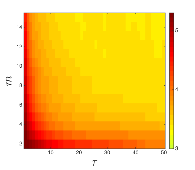
(a) SPI values for different delay reconstructions of a representative trace from the Lorenz 96 system with $\{K=22,F=5\}$.

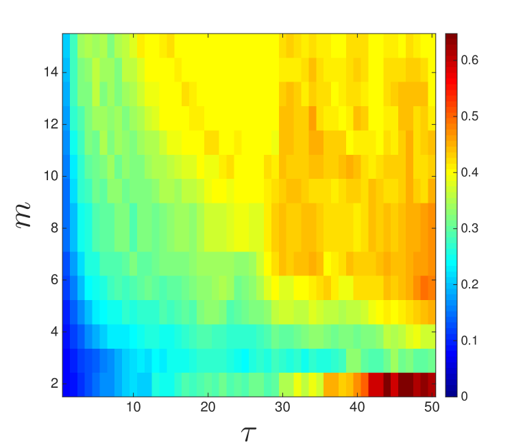
(b) MASE scores for LMA forecasts on different delay reconstructions of a representative trace of the Lorenz 96 system with $\{K=22,F=5\}$.

Figure 4: The effects of reconstruction parameter values on SPI and forecast accuracy for the Lorenz 96 system

Not surprisingly, this image reveals a strong dependency between the values of the reconstruction parameters and the reduction in uncertainty about the near future that is provided by the reconstruction. Very low $\tau$ values, for instance, produce delay vectors with highly redundant coordinates, but which provide substantial information about the future. As mentioned in the first section of this paper, standard heuristics only focus on minimizing redundancy between coordinates and choose the $\tau$ value that minimizes the mutual information between the first two coordinates in the delay vector. For this trajectory, the approach of Fraser & Swinneyfraser-swinney yields $\tau=26$, while standard dimension-estimation heuristics KBA92 suggest $m=8$. The SPI value for a delay reconstruction built with those parameter values is 3.463. This is not, however, the SPI-optimal reconstruction; choosing $m=2$ and $\tau=1$, for instance, results in a higher value ($SPI=5.303$)—i.e., signficantly more reduction in uncertainty about the future. This may be somewhat counter-intuitive, since each of the delay vectors in the SPI-optimal reconstruction spans far less of the data set and thus one would expect points in that space to contain less information about the future. Figure 4(a) suggests, however, that this in fact not the case; rather, that uncertainty increases with both dimension and time delay.

The question at issue in this paper is whether that reduction in uncertainty about the future correlates with improved accuracy of an LMA forecast built from that reconstruction. Since the SPI-optimal choices maximize the shared information between the state estimator and $X_{j+1}$, one would expect a delay reconstruction model built with those choices to afford LMA the best leverage. To test that conjecture, we performed an exhaustive search with $m=2,\dots,15$ and $\tau=1,\dots,50$. For each $\{m,\tau\}$ pair, we used LMA to generate forecasts from the corresponding reconstruction, computed their $MASE$ scores, and plotted the results in a heatmap similar to the one in Figure 4(a). As one would expect, the $MASE$ and SPI heatmaps are generally antisymmetric. This antisymmetry breaks down somewhat for low $m$ and high $\tau$, where the forecast accuracy is low even though the reconstruction contains a lot of information about the future. We suspect that this is due to a combination of overfolding (due to too-large values of $\tau$) and projection (low $m$). Even though each point in such a reconstuction may contain a lot of information about the future, the false crossings created by this combination of effects pose problems for a near-neighbor forecast strategy like LMA. The improvement that occurs if one adds another dimension is consistent with this explanation. Notice, too, that this effect only occurs far from the maximum in the SPI surface—the area that is of interest if one is using SPI to choose parameter values for reconstruction models.

In general, though, maximizing the redundancy between the state estimator and the future does appear to minimize the resulting forecast error of LMA. Indeed, the maximum on the surface of Figure 4(b) ($m=2,\tau=1$) is exactly the minimum on the surface of Figure 4(a). The accuracy of this forecast is more than five times higher ($MASE=0.0737$) than that of a forecast constructed with the parameter values suggested by the standard heuristics ($0.3787$). Note that the optima of these surfaces may be broad: i.e., there may be ranges of $m$ and $\tau$ for which SPI and $MASE$ are optimal, and roughly constant. In these cases, it makes sense to choose the lowest $m$ on the plateau, since that minimizes computational effort, data requirements, and noise effects; see joshua-pnp for a full discussion of this.

While the results discussed in the previous paragraph do provide a preliminary validation of the claim that one can use SPI to select good parameter values for delay reconstruction-based forecast strategies, they only involve a single example system. Similar experiments on traces from the Lorenz 96 system with different parameter values $\{K=47,F=5\}$ show identical results—indeed, the heatmaps are visually indistinguishable from the ones in Figure 4. Figure 5 shows heatmaps of SPI and $MASE$ for similar experiments on the classic “Lorenz 63” systemlorenz :

$$\dot{x} = \sigma(y-x)$$

$$\dot{y} = x(\rho-z)-y$$

$$\dot{z} = xy-\beta z$$

with the typical chaotic parameter selections: $\rho=28,\sigma=10$, and $\beta=8/3$.

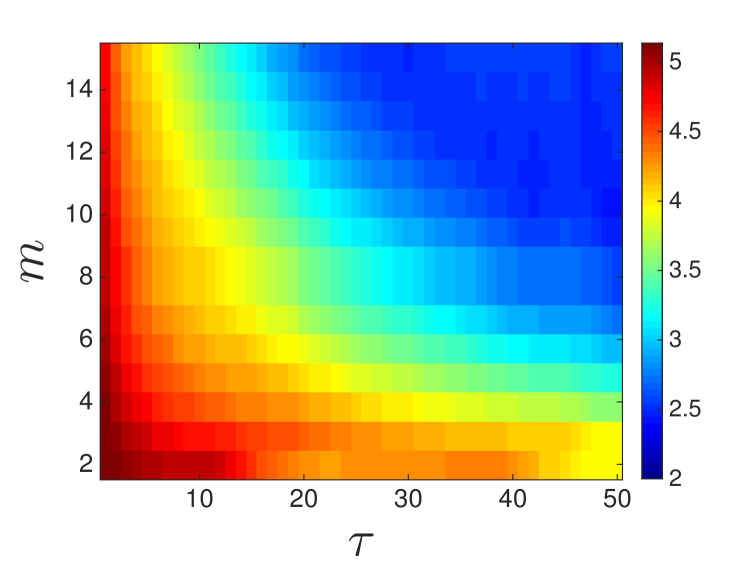
(a) SPI values for different delay reconstructions of a representative trace from the Lorenz 63 system.

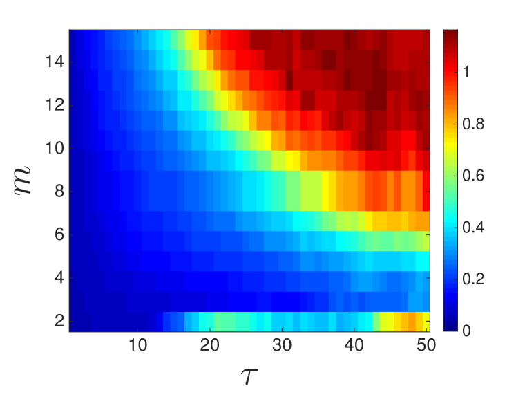
(b) $MASE$ scores for LMA forecasts on different delay reconstructions of a representative trace of the Lorenz 63 system.

Figure 5: The effects of reconstruction parameter values on SPI and forecast accuracy for the Lorenz 63 system

As in the Lorenz 96 case, the heatmaps are generally antisymmetric, confirming that maximizing SPI is roughly equivalent to minimizing $MASE$. Again, though, the antisymmetry is not perfect; for high $\tau$ and low $m$, the effects of projecting an overfolded attractor cause false crossings that trip up LMA. As before, adding a dimension mitigates this effect by removing these false crossings. Both the Lorenz 63 and Lorenz 96 plots show a general decrease in predictability for large $m$ and high $\tau$, with roughly hyperbolic equipotentials dividing the colored regions. The locations and heights of these equipotentials differs because the two signals are not equally easy to predict. This matter is discussed further at the end of this section.

Numerical SPI and $MASE$ values for LMA forecasts on different reconstructions of both Lorenz systems are tabulated in the top three rows of Table 1, along with the reconstruction parameter values that produced those results.

Table 1: $MASE$ values for various delay reconstructions of the different examples studied here. $MASE_{H}$ is the representative accuracy of LMA forecasts that use delay reconstructions with parameter values ($m_{SPI}$ and $\tau_{SPI}$) chosen via standard heuristics for the corresponding traces—the methods of false neighbors KBA92 and time-delayed mutual information fraser-swinney , respectively. Similarly, $MASE_{SPI}$ is the accuracy of LMA forecasts that use reconstructions built with the $m$ and $\tau$ values that maximize SPI, and $MASE_{E}$ is the error of the best forecasts for each case, found via exhaustive search over the $m,\tau$ parameter space. ${**}$: on these signals the standard heuristics failed.

Signal	$MASE_{H}$	$\tau_{H}$	$m_{H}$	$MASE_{SPI}$	$\tau_{SPI}$	$m_{SPI}$	$MASE_{E}$	$\tau_{E}$	$m_{E}$
Lorenz-96 $K=22$	0.3787	26	8	0.0737	1	2	0.0737	1	2
Lorenz-96 $K=47$	1.007	31	10	0.1156	1	2	0.1156	1	2
Lorenz 63	0.2215	12	5	0.0509	1	3	0.0506	1	2
Hénon Map	∗∗	∗∗	∗∗	3.814e-04	1	2	3.814e-04	1	2
Logistic Map	∗∗	∗∗	∗∗	1.680e-05	1	1	1.680e-05	1	1

The data in this table bring out two important points. First, as suggested by the heatmaps, the $m$ and $\tau$ values that maximize SPI (termed $m_{SPI}$ and $\tau_{SPI}$ in the table legend) are close, or identical, to the values that minimize $MASE$ ($m_{E}$ and $\tau_{E}$) for all three Lorenz systems. This is notable because—as discussed in Section V.1—the former can be estimated quite reliably from a small sample of the trajectory in only a few seconds of compute time, whereas the exhaustive search that is involved in computing $m_{E}$ and $\tau_{E}$ for Table 1 required close to 30 hours of CPU time per signal. A second important point that is apparent from the Table is that delay reconstructions built using the traditional heuristics—the values with the $H$ subscript—were comparatively ineffective for the purposes of LMA-based forecasting. This is notable because that is the default approach in the literature on state-space based forecasting methods for dynamical systems.

A close comparison of Figures 4 and 5 brings up another important point: some time series are harder to forecast than others. Figure 6 breaks down the details of the two suites of Lorenz-96 experiments, showing the distribution of SPI and $MASE$ values for all of the reconstructions.

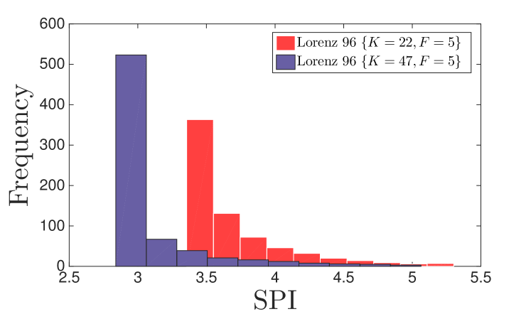
(a) SPI

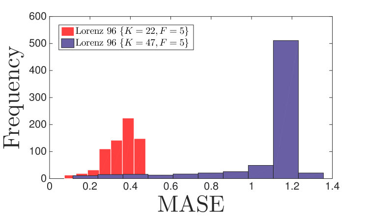
(b) $MASE$

Figure 6: Histograms of SPI and $MASE$ values for representative traces from the Lorenz 96 $\{K=22,F=5\}$ and $\{K=47,F=5\}$ systems for all $\{m,\tau\}$ values in Figures 4 and 5.

Although there is some overlap in the $K=47$ and $K=22$ histograms—i.e., best-case forecasts of the former are better than most of the forecasts of the latter—the $K=47$ traces generally contain less information about the future and thus are harder to forecast accurately.

IV.1.2 Map examples

Delay reconstruction of discrete-time dynamical systems, while possible in theory, can be problematic in practice. Although the embedding theorems do apply in these cases, the heuristics for estimating $m$ and $\tau$ often fail. The time-delayed mutual information of fraser-swinney , for example, may decay exponentially, without showing any clear minimum. And the lack of spatial continuity of the orbit of a map violates the underlying idea behind the method of KBA92 . State space-based forecasting methods can, however, be very useful in generating predictions of trajectories from systems like this—if one has a reconstruction that is faithful to the true dynamics.

In view of this, it would be particularly useful if one could use SPI to choose embedding parameter values for maps. This section explores that notion using two canonical examples, shown in the bottom two rows of Table 1. For the Hénon map,

$$x_{n+1} = 1-ax^{2}_{n}+y_{n}$$

$$y_{n+1} = bx_{n}$$

with $a=1.4$ and $b=0.3$, the SPI-optimal parameter values were $m=2$ and $\tau=1$. As in the flow examples, these were identical to the values that minimized $MASE$. These parameter values make sense, of course; a first-return map of the $x$ coordinate is effectively the Hénon map, so $[x_{j},x_{j-1}]$ is a perfect state estimator (up to a scaling term). But in practice, of course, one rarely knows the underlying dynamics of the system that generated a time series, so the fact that one can choose good reconstruction parameter values by maximizing SPI is notable—especially since standard heuristics for that purpose fail in this system.

The same pattern holds for the logistic map, $x_{n+1}=rx_{n}(1-x_{n})$, with $r=3.65$: the SPI-optimal parameter values coincide with the minimum of the $MASE$ surface. As in the Hénon example, these values ($m=1$ and $\tau=1$) make complete sense, given the form of the map. But again, one does not always know the form of the system that generated a given time series. In the case of the logistic map, the standard heuristics fail, but SPI clearly indicates that one does not actually need to reconstruct these dynamics—rather, near-neighbor forecasting on the time series itself is the best approach.

IV.2 Selecting reconstruction parameters of experimental time series

The results in the previous section provide a preliminary verification of the conjecture that maximizing SPI minimizes forecast accuracy of LMA, for both maps and flows. While experiments with synthetic examples are useful, they do not call the really important aspect of that research question: whether SPI is a useful way to choose parameter values for delay reconstruction-based forecasting of real-world data, where the time series are noisy and perhaps short, and one does not know the dimension of the underlying system—let alone its governing equations. In this section, we turn our attention to that question using experimental data from two different dynamical systems: a far-infrared laser and a laboratory computer-performance experiment.

IV.2.1 A Far-Infrared Laser

A canonical test case in the forecasting literature is the so-called “Dataset A” from the Santa Fe Institute prediction competitionweigend-book , which was gathered from a far-infrared laser. As in the synthetic examples in the previous section, the SPI and $MASE$ heatmaps (Figure 7) are largely antisymmetric for this signal.

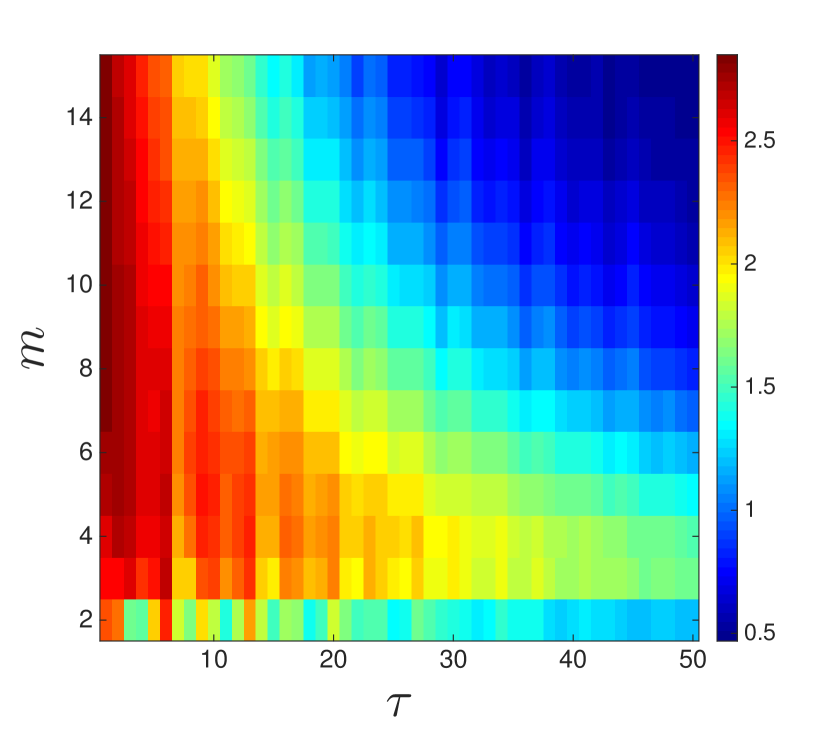
(a) SPI values for different delay reconstructions of SFI Dataset A.

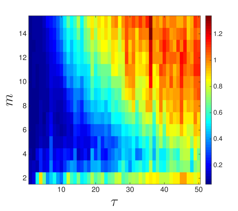
(b) MASE scores for LMA forecasts on different delay reconstructions of SFI Dataset A.

Figure 7: The effects of reconstruction parameter values on SPI and forecast accuracy for “Dataset A” from the Santa Fe Institute time-series prediction competition.

Again, there is a band across the bottom of each image because of the combined effects of overfolding and projection. Note the resemblance between Figures  7 and  5: the latter resemble “smoothed” versions of the former. It is well knownweigend-book that the SFI A dataset is well described by the Lorenz 63 system with some added noise, so this similarity is both unsurprising and reassuring. LMA forecasts using the SPI-optimal reconstruction of this trace were more accurate than similar forecasts using a reconstruction built using traditional heuristics ($MASE_{SPI}=0.0592$ versus $MASE_{H}=0.0733$) and only slightly worse than the optimal value ($MASE_{E}=0.0538$). However, the values of $\{m_{SPI},\tau_{SPI}\}$ and $\{m_{E},\tau_{E}\}$ are not identical for this signal. This is because the optima in the heatmaps in Figure 7 are bands, rather than unique points—as was the case in the synthetic examples in Section IV.1. In a situation like this, a range of $\{m,\tau\}$ values are statistically indistinguishable, from the standpoint of the forecast accurary afforded by the corresponding reconstruction. The values suggested by the SPI calculation ($m_{SPI}=9$ and $\tau_{SPI}=1$) and by the exhaustive search ($m_{E}=7$, $\tau_{E}=1$) were all on this plateau. Again, it appears that one can use SPI to choose good parameter values for delay reconstruction-based forecasting, but SFI A is only a single trace from a fairly simple system.

IV.2.2 Computer Performance Dynamics

Laboratory experiments on computer performance dynamics have shown that these high-dimensional nonlinear systems exhibit a range of interesting deterministic dynamical behaviorszach-IDA10 ; mytkowicz09 . Both hardware and software play roles in these dynamics; changing either one can cause bifurcations from periodic orbits to low- and high-dimensional chaos. This rich range of behavior makes computer performance dynamics an ideal final test case for this paper.

Collecting observations of the performance of a running computer requires some significant engineering. Basically, one programs the microprocessor’s onboard hardware performance monitor to observe the quantities of interest, then stops the program execution at 100,000-instruction intervals—the unit of time in these experiments—and reads off the contents of those registers. Interested readers can find a detailed description of this custom measurement infrastructure intodd-phd ; mytkowicz09 . The signals that are produced by this apparatus are scalar time-series measurements of system metrics like processor efficiency (e.g., IPC, which measures how many instructions are being executed, on the average, in each clock cycle) or memory usage (e.g., how often the processor had to access the main memory during the measurement interval).

Here, for conciseness, we focus on processor performance traces from two different programs, one simple and one complex, running on the same Intel i7-based computer. The first is four lines of C (col_major) that repeatedly initializes a $256\times 256$ matrix in column-major order. The second is a much more complex program: the 403.gcc compiler from the SPEC 2006CPU benchmark suitespec2006 . The performance traces of these two programs contained 147,925 points and 45,545 points, respectively. Since computer performance dynamics result from a composition of hardware and software, these two experiments involve two different dynamical systems, even though the programs are running on the same computer. But since other effects could be at work—housekeeping by the operating system, etc.—we repeated each experiment 15 times for a total of 30 traces. We have performed similar forecast experiments using other processor and memory performance metrics gathered during the execution of a variety of programs on several different computers josh-pre . Our preliminary analysis indicates that the results described in the rest of this section hold for those traces as well.

As in the previous examples, heatmaps of $MASE$ and SPI for the col_major time series (Figure 8(b)) are largely antisymmetric.

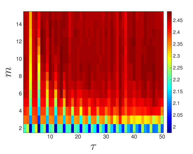
(a) SPI values for different delay reconstructions of a col_major trace.

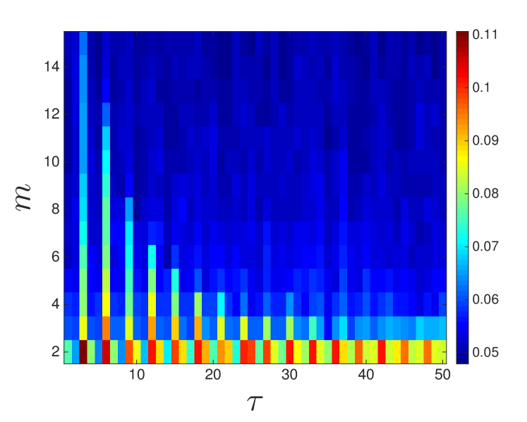
(b) $MASE$ scores for LMA forecasts on different delay reconstructions of a col_major trace.

Figure 8: The effects of reconstruction parameter values on SPI and forecast accuracy for a representative trace from a computer-performance dynamics experiment tracing the processor load during the execution of a simple program that repeatedly initializes a matrix in column-major order.

And again, reconstructions using the SPI-optimal parameter values allowed LMA to produce highly accurate forecasts of this signal: $MASE_{SPI}=0.0509$, compared to the optimal $MASE_{E}=0.0496$. There are several major differences between these plots and the previous ones in this paper, though, beginning with the vertical stripes. These are due to the dominant unstable periodic orbit of period 3 in the chaotic attractor in the col_major dynamics. When $\tau$ is a multiple of this period ($\tau=3\kappa$), the coordinates of the delay vector are not independent, which lowers SPI and makes forecasting more difficult. (There is a nice theoretical discussion of this effect in sauer91 .) Conversely, SPI spikes and $MASE$ plummets when $\tau=3\kappa-1$, since the coordinates in such a delay vector cannot share any prime factors with the period of the orbit. The band along the bottom of both images is, again, due to a combination of overfolding and projection.

Another difference between the col_major heatmaps and the ones in Figures 4, 5, and 7 is the apparent overall trend: the “good” regions (low $MASE$ and high SPI) are in the lower-left quadrants of those heatmaps, but in the upper-right quadrant of Figure 8. This is partly an artifact of the difference in the color-map scale, which was chosen here to bring out some important details of the structure, and partly due to that structure itself. Specifically, the optima of the col_major heatmaps—the large dark red and blue regions in Figures 8(a) and 8(b), respectively—are much broader than the ones in the earlier sections of this paper, perhaps because the signal is so close to periodic. (This was also the case to some extent in the SFI A example, for the same reason.) This geometry makes precise comparisons of SPI-optimal and $MASE$-optimal parameter values somewhat problematic, as the exact optima on two almost-flat but slightly noisy landscapes may not be in the same place. Indeed, the SPI values at $\{m_{SPI},\tau_{SPI}\}$ and $\{m_{E},\tau_{E}\}$ were within a standard error across all 15 traces of col_major.

And that brings up an interesting tradeoff. For practical purposes, what one wants is $\{m_{SPI},\tau_{SPI}\}$ values that produce a $MASE$ value that is close to the optimum $MASE_{E}$. However, the algorithmic complexity of most nonlinear time-series analysis and prediction methods scales badly with $m$. In cases where the SPI maximum is broad, then, one might want to choose the lowest value of $m$ on that plateau—or even a value that is on the shoulder of that plateau, if one needs to balance efficiency over accuracy. Indeed, forecasts with $m=2$ appear to work surprisingly well for many nonlinear dynamical systems, including the col_major datajoshua-pnp . Fixing $m=2$ amounts to marginalizing the heatmaps in Figure 8, which produces a cross section like the ones shown in Figure 9.

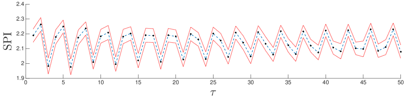
(a) SPI values for delay reconstructions of the col_major traces with $m=2$ and a range of values of $\tau$.

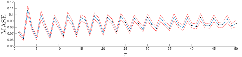
(b) $MASE$ scores for LMA forecasts of delay reconstructions of the col_major traces with $m=2$ and a range of values of $\tau$.

Figure 9: $MASE$ and SPI for LMA forecasts of $m=2$ delay reconstructions of all 15 col_major traces, plotted as a function of $\tau$. The blue dashed curves show the averages across all trials; the red dotted lines are that average $\pm$ the standard deviation.

The antisymmetry between SPI and $MASE$ is quite apparent in these plots; the global maximum of the former coincides with the global minimum of the latter, at $\tau=2$. The average $MASE$ score of col_major forecasts constructed with $m=2$ and this $\tau$ value is $0.0649$. This is not much lower than the overall optimum of 0.0496—a value from a forecast whose free parameters required almost six orders of magnitude more CPU time to compute. As an important aside: these results suggest that one could bypass even more of the computational effort that is involved in delay reconstruction-based forecasting by simply working in two dimensions, i.e., by calculating SPI across a range of $\tau$s, rather than across a 2D $\{m,\tau\}$ space. This approach is discussed further in joshua-pnp .

The correspondence between $MASE$ and SPI also holds true for other marginalizations: i.e., the minimum $MASE$ and the maximum SPI occur at the same $\tau$ value for all $m$-wise slices of the col_major heatmaps, to within statistical fluctuations. The methods of fraser-swinney and KBA92 , incidentally, suggest $\tau_{H}=2$ and $m_{H}=12$ for these traces; the $MASE$ of an LMA forecast on such a reconstruction is 0.0530, which is somewhat better than the best result from the $m=2$ marginalization, although still short of the overall optimum. The correspondence between $\tau_{H}$ and $\tau_{SPI}$ is coincidence; for this particular signal, maximizing the independence of the coordinates happened to maximize the information about the future contained in each delay vector. The $m=12$ result is not coincidence—and quite interesting, in view of the fact that the $m=2$ forecast is so good. It is also surprising in view of the huge number of transistors—potential state variables—in a modern computer. As described in mytkowicz09 , however, the hardware and software constraints in these systems confine the dynamics to a much lower-dimensional manifold. All of these issues, and their relation to the task of prediction, are explored in more depth in joshua-pnp .

The col_major program is what is known in the computer-performance literature as a “micro-kernel”—a extremely simple example that is used in proof-of-concept testing. The fact that its dynamics are so rich speaks to the complexity of the hardware (and the hardware-software interactions) in modern computers; again, see todd-phd ; mytkowicz09 for a much deeper discussion of these issues. Modern computer programs are far more complex than this simple micro-kernel, of course, which begs the question: what does SPI tell us about the dynamics of truly complex systems like that—programs that the computer-performance community models as stochastic systems?

For 403.gcc, the answer is, again, that SPI appears to be an effective and efficient way to assess predictability. It has been shownjosh-pre that this time series shares little to no information with the future: i.e., that it cannot be predicted using delay reconstruction-based forecasting methods, regardless of $\tau$ and $m$ values. The experiments in josh-pre required dozens of hours of CPU time to establish that conclusion; SPI gives the same results in a few seconds, using much less data. The structure of the heatmaps for this experiment, which are shown in Figure 10, is radically different.

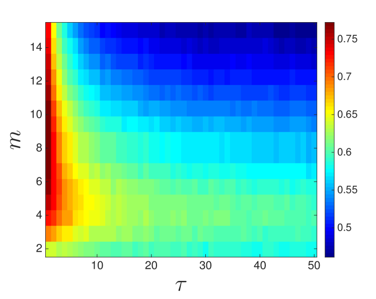
(a) SPI values for different delay reconstructions of a 403.gcc trace.

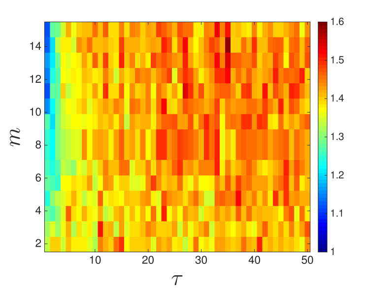
(b) $MASE$ scores for LMA forecasts on different delay reconstructions of a 403.gcc trace.

Figure 10: The effects of reconstruction parameter values on SPI and forecast accuracy for a representative trace from a computer-performance dynamics experiment using the 403.gcc benchmark

The patterns visible in the previous $MASE$ plots, and the antisymmetry between SPI and $MASE$ plots, are absent from Figure 10, reflecting the lack of predictive content in this signal. Note, too, that the color maps are different in this Figure. This reflects the much lower values of SPI for this signal: a maximum SPI of 0.7722 for 403.gcc, compared to 5.3026 for Lorenz 96 with $K=22$. Indeed, the $MASE$ surface in Figure 10(b) never dips below 1.0. That is, regardless of parameter choice, LMA forecasts of 403.gcc are no better than simply using the prior value of this scalar time series as the prediction. The uniformly low SPI values in Figure 10(a) are an effective indicator of this—and, again, they can be calculated quickly, from a relatively small sample of the data. It is to that issue that we turn next.

V Data Requirements and Prediction Horizons

In some real-world situations, it may be impractical to rebuild forecast models at every step, as we have done in the previous sections of this paper—because of computational expense, for instance, or because the data rate is very high. In these situations, one may wish to predict $p$ time steps into the future, then stop and rebuild the model to incorporate the $p$ points that have arrived during that period, and repeat. In chaotic systems, of course, there are fundamental limits on prediction horizon even if one is working with infinitely long traces of all state variables. A key question at issue in this section is how that effect plays out in forecast models that use delay reconstructions from scalar time-series data. And since real-world data sets are not infinitely long, it is important to understand the effects of data length on the estimation of SPI.

V.1 Data Requirements for SPI Estimation

The quantity of data used in a delay reconstruction directly impacts the usefulness of that reconstruction. If one is interested in approximating the correlation dimension via the Grassberger-Procaccia algorithm, for instance, it has been shown that one needs $10^{(2+0.4m)}$ data pointstsonisdatabound ; smithdatabound . Those bounds are overly pessimistic for forecasting, however. For example, Sugihara & May sugihara90 used delay-coordinate reconstructions with $m$ as large as seven to successfully forecast biological and epidemiological time-series data sets that contain as few as 266 points. A key challenge, then, is to determine whether one’s time series really calls for as many dimensions and data points as the theoretical results require, or whether one can get away with fewer dimensions—and how much data one needs in order to figure all of that out.

We claim that SPI is a useful solution to those challenges. As established in the previous sections, calculations of this quantity can reveal what dimension one needs to build a good delay reconstruction for the purposes of LMA forecasting of nonlinear and chaotic systems. And, as alluded to in those sections, SPI can be estimated accurately from a surprisingly small number of points. The experiments in this section explore that intertwined pair of claims in more depth by increasing the length of the Lorenz 96 traces and testing whether the information content of the state estimator derived from standard heuristics converges to the SPI-optimal estimator.

Figure 11 shows the results.

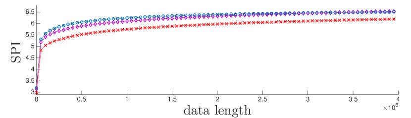
(a) Optimal SPI for traces from the $\{K=22,F=5\}$ Lorenz 96 system

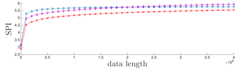
(b) Optimal SPI for traces from the $\{K=47,F=5\}$ Lorenz 96 system

Figure 11: SPI versus data length for traces from the Lorenz-96 system using $\tau=1$ in all cases. Blue circles corresponds to an embedding dimension $m=2$, purple diamonds to $m=4$, and red xs to $m=8$.

When the data length is short, the $m=2$ state estimator had the most information about the future. This makes perfect sense; a short time series cannot fully sample a complicated object, and when an ill-sampled high-dimensional manifold is projected into a low dimensional space, infrequently visited regions of that manifold can act effectively like noise. From an information-theoretic standpoint, this would increase the effective Shannon entropy rate of each of the variables in the delay vector. In the I-diagram in Figure 3, this would manifest as drifting apart of the two circles, decreasing the shaded region that one needs to maximize for effective forecasting.

If that reasoning is correct, longer data lengths should fill out the attractor, thereby mitigating the spurious increase in the Shannon entropy rate and allowing higher-dimensional reconstructions to outperform lower-dimensional ones. This is indeed what one sees in Figure 11. For both the $K=22$ and $K=47$ traces, once the signal is 2 million points long, the four-dimensional estimator has caught up to and even exceeded the two-dimensional case. Note, though, that the optimal SPI of the $m=8$ reconstruction model is still lower than in the $m=2$ or $4$ cases, even at the right-hand limit of the plots in Figure 11. That is, even with a time series that contains $4\times 10^{6}$ points, it is more effective to use a lower dimensional reconstruction to make an LMA forecast. But the really important message here is that SPI allows one to determine the best reconstruction parameters for the available data, which is an important part of the answer to the challenges outlined at the beginning of this section.

Something very interesting happens in the $m=2$ results for Lorenz 96 model with $K=47$: the SPI curve reaches a maximum value around 100,000 points and stops increasing, regardless of data length. What this means is that this two-dimensional reconstruction contains as much information about the future as can be ascertained from these data, suggesting that increasing the length of the training set would not improve forecast accuracy. To explore this, we constructed LMA forecasts of different-length traces (100,000–2.2 million points) from this system, then reconstructed their dynamics with different $m$ values and the appropriate $\tau_{SPI}$ for each case. For $m=2$, both SPI and $MASE$ results did indeed plateau at 100,000 points—at 5.736 and 0.0809, respectively. As before, more data does afford higher-dimensional reconstructions more traction on the prediction problem: the $m=4$ forecast accuracy surpassed $m=2$ at around 2 million points ($MASE=0.0521$). In neither case, by the way, did $m=8$ catch up to either $m=2$ or $m=4$, even at 4 million data points. Of course, one must consider the cost of storing the additional variables in a higher-dimensional reconstruction model, particularly in data sets this long, so it may be worthwhile in practice to settle for the $m=2$ forecast—which is only slightly less accurate and requires only 100,000 points. This has another major advantage as well. If the time series is non-stationary, a forecast strategy that requires fewer points can adapt more quickly.

V.2 Choosing reconstruction parameters for increased prediction horizons.

So far in this paper, we have considered forecasts that were constructed one step at a time and studied the correspondence of their accuracy with one-step-ahead calculations of SPI. In this section, we consider longer prediction horizons ($p$) and explore whether one can use a $p$-step-ahead version of SPI—i.e., $I[\mathcal{S}_{j},X_{j+p}]$, with $p>1$—to choose parameter values that maximize the information contained in each delay vector about the value of the time series $p$ steps in the future.

One would expect the SPI-optimal $\{m,\tau\}$ values for a given time series to depend on the prediction horizon. It has been shown, for instance, that longer-term forecasts generally do better with larger $\tau$kantz97 , and converselyjoshua-pnp . It makes sense that one might need to reach different distances into the past (via the span of the delay vector) in order to reduce the uncertainty about events that are further into the futureweigend-book . These effects are corroborated by SPI. Figure 12 demonstrates this in the context of the Lorenz 96 system with $K=22$, focusing on $m=2$ for simplicity.

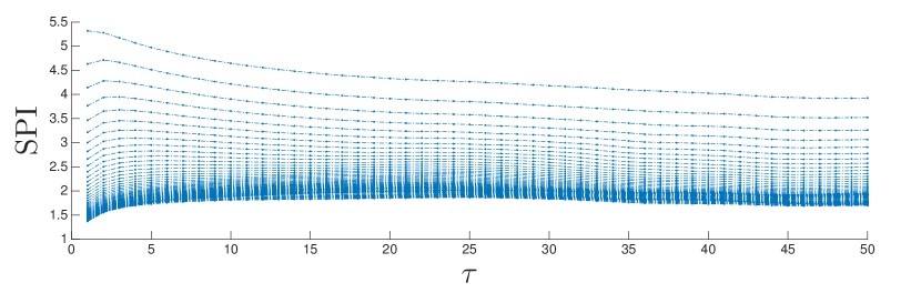
Figure 12: The effect of prediction horizon ($p$) on SPI of the $K=22$ Lorenz 96 system for a fixed reconstruction dimension ($m=2$). The traces in the image, starting from the top, correspond to prediction horizons of $p=1$ to $p=100$.

The topmost trace in this figure is for the $p=1$ case—i.e., a horizontal slice of Figure 4(a) made at $m=2$. The maximum of this curve is the optimal $\tau$ value ($\tau_{SPI}$) for this reconstruction. The overall shape of this trace reflects the monotonic increase in the uncertainty about the future with $\tau$ that is noted on page 4. The other traces in Figure 12 show SPI as a function of $\tau$ for $p=2,3,\dots$, down to $p=100$ at the bottom of the figure. The lower traces do not decrease monotonically; rather, there is a slight initial rise. This is due to the point made above about the span of the delay vector: if one is predicting further into the future, it may be useful to reach further into the past. In general, this causes the optimal $\tau$ to shift to the right as prediction horizon increases, going down the plot—i.e., longer prediction horizons require a greater $\tau$ (cf. kantz97 ). For very long horizons, the choice of $\tau$ appears to matter very little. In particular, SPI is fairly constant and quite low for $5<\tau<50$ when $p>30$—i.e., regardless of the choice of $\tau$, there is very little information about the $p$-distant future in any delay reconstruction of this signal for $p>30$. This effect should not be surprising, and it is well corroborated in the literature. However, it can be hard to know a priori, when one is confronted with a data set from an unknown system, to know what prediction horizon makes sense. SPI offers a computationally efficient way to answer that question.

Figure 13 shows a similar exploration of the other side of that question: the effects of the reconstruction dimension on SPI, with $\tau$ fixed at 1.

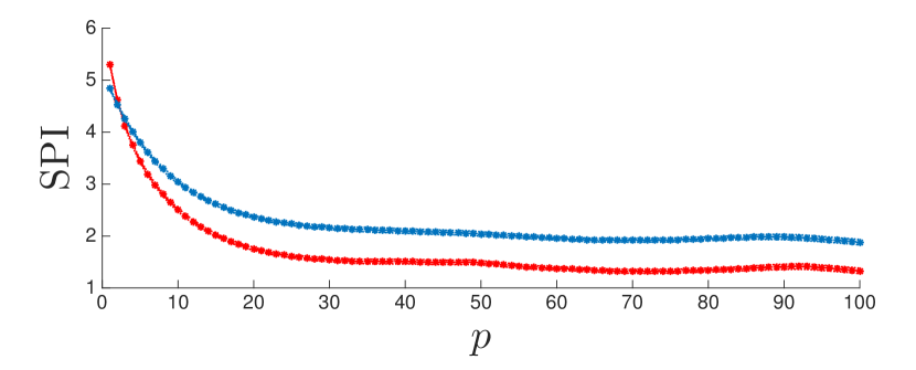
Figure 13: The effect of prediction horizon ($p$) on SPI of the $K=22$ Lorenz 96 system for a fixed time delay ($\tau=1$) and two different reconstruction dimensions. The red line is $m=2$ and the blue is $m_{H}=8$, the value suggested for this signal by the technique of false neighbors.

The $m=2$ state estimator contains more information about the future for short prediction horizons. This ties back to the discussion at the end of Section IV.2.2: low-dimensional reconstructions can work quite well for short prediction horizons. However, Figure 13 shows that the full reconstruction is better for longer horizons. This is not terribly surprising, since a higher reconstruction dimension allows the state estimator to capture more information about the past. Finally, note that SPI decreases monotonically with prediction horizon for both $m=2$ and $m_{H}$. This, too, is unsurprising. Pesin’s relationpesin1977characteristic says that the sum of the positive Lyapunov exponents is equal to the entropy rate, and if there is a non-zero entropy rate, then generically observations will become increasingly independent the further apart they are. This explanation also applies to Figure 12, of course, but it does not hold for signals that are wholly (or nearly) periodic.

Recall that the col_major dynamics in Section IV.2.2 were chaotic, but with a dominant unstable periodic orbit—which had a variety of interesting effects in the results. Figure 14 explores the effects of prediction horizon on those results.

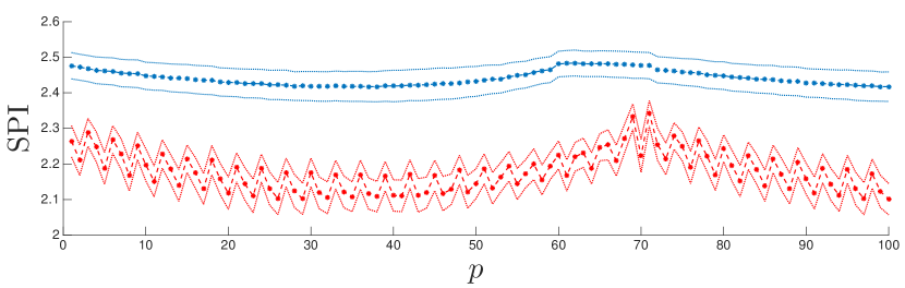
Figure 14: The effect of prediction horizon ($p$) on SPI of the col_major for a fixed time delay ($\tau=1$) and two different reconstruction dimensions. The red line is $m=2$ and the blue is $m_{H}=12$, the value suggested for this signal by the technique of false neighbors.

Not surprisingly, there is some periodicity in the SPI versus $p$ relationships, but not for the same reasons that caused the stripes in Figure 8(b). Here, the peaks in SPI occur at multiples of the period. That is, the $m=2$ state estimator can forecast with the most success when the value being predicted is in phase with the delay vector. Note that this effect is far stronger for $m=2$ than $m_{H}$, simply because of the instability of that periodic orbit; the visits made by the chaotic trajectory to that orbit are more likely to be short than long. As expected, SPI decays with prediction horizon—but only at first, after which it begins to rise again, peaking at $p=69$ and $p=71$. This may be due to a second higher-order unstable periodic orbit in the col_major dynamics.

In theory, one can derive rigorous bounds on prediction horizon. The time at which $\mathcal{S}_{j}$ will no longer have any information about the future can be determined by considering:

$$R(p)=\frac{I[\mathcal{S}_{j};X_{j+p}]}{H[X_{j+p}]}~{},$$

i.e., the percentage of the uncertainty in $X_{j+p}$ that can be reduced by the delay vector. Generically, this will limit to some small value equal to the amount of information that the delay vector contains about any arbitrary point on the attractor. Given some criteria regarding how much information above the “background” is required of the state estimator, one could use the $R(p)$ versus $p$ to determine the maximum practical horizon.

In practice, one can select parameters for delay reconstruction-based forecasting by explicitly including the prediction horizon in the SPI function, fixing its value at the required value, performing the same search as we did in earlier sections over a range of $m$ and $\tau$, and then choosing a point on (or near) the optimum of that SPI surface. The computational and data requirements of this calculation, as shown in Section V.1, are far superior to those of the standard heuristics used in delay reconstructions.

VI Conclusion

In this paper, we have described a new metric for quantifying how much information about the future is contained in a delay reconstruction. Using a number of different dynamical systems, we demonstrated a direct correspondence between the SPI value for different delay reconstructions and the accuracy of forecasts made with Lorenz’s method of analogues on those reconstructions. Since SPI can be calculated quickly and reliably from a relatively small amount of data, without needing to know anything about the governing equations or the state space dynamics of the system, that correspondence is a major advantage, in that it allows one to choose parameter values for delay reconstruction-based forecast models without doing an exhaustive search on the parameter space. Significantly, SPI-optimal reconstructions are better, for the purposes of forecasting, than reconstructions constructed using standard heuristics like mutual information and the method of false neighbors, which can require large amounts of data, significant computational effort, and expert human interpretation. SPI allows us to answer other questions regarding forecasting with theoreticaly unsound modelsjoshua-pnp —e.g., why one can obtain a better forecast using a low-dimensional reconstruction than with a full embedding. It also allows one to understand bounds on prediction horizon without having to estimate Lyapunov spectra or Shannon entropy rates, which are difficult to obtain for arbitrary real-valued time series. That, in turn, allows one to tailor one’s reconstruction parameters to the amount of available data and the desired prediction horizon—and to know if a given prediction task is just not possible.

The explorations in this paper involve a simple near-neighbor forecast strategy and state estimators that are basic delay reconstructions of raw time-series data. The definition and calculation of SPI do not involve any assumptions about the state estimator, though, so the results presented here should also hold for other state estimators. For example, it is common in time-series prediction to pre-process one’s data: for example, low-pass filtering or interpolating to produce additional points. Calculating SPI after performing such an operation will accurately reflect the amount of information in that new time series—indeed, it would reveal if that pre-processing step destroyed information. And we believe that the basic conclusions in this paper extend to other state-space based forecast schemas besides Lorenz’s method of analogues, such as those used in weigend-book ; casdagli-eubank92 ; Smith199250 ; sugihara90 ; sauer-delay —although SPI may not accurately select optimal parameter values for strategies that involve post-processing the data (e.g., GHKSSghkss ). We are in the process of exploring this.

There are many other interesting potential ways to leverage SPI in the practice of forecasting. If the SPI-optimal $\tau=1$, that may be a signal that the time series is undersampling the dynamics and that one should increase the sample rate. One could use SPI at a finer grain to optimizing $\tau$ individually for each dimension, as suggested in pecoraUnified . To do this, one could define $\mathcal{S}_{j}=[X_{j},X_{j-\tau_{1}},X_{j-\tau_{2}},\dots,X_{j-\tau_{m-1}}]$ and then simply maximize SPI using that state estimator constrained over $\{\tau_{i}\}_{i=1}^{m-1}$.

VII References

References

- (1) F. Takens, Detecting strange attractors in fluid turbulence, in: D. Rand, L.-S. Young (Eds.), Dynamical Systems and Turbulence, Springer, Berlin, 1981, pp. 366–381.
- (2) N. Packard, J. Crutchfield, J. Farmer, R. Shaw, Geometry from a time series, Physical Review Letters 45 (1980) 712.
- (3) T. Sauer, J. Yorke, M. Casdagli, Embedology, Journal of Statistical Physics 65 (1991) 579–616.
- (4) E. Olbrich, H. Kantz, Inferring chaotic dynamics from time-series: on which length scale determinism becomes visible, Phys. Lett. A 232 (1-2) (1997) 63–69.
- (5) A. Fraser, H. Swinney, Independent coordinates for strange attractors from mutual information, Physical Review A 33 (2) (1986) 1134–1140.
- (6) H. Kantz, T. Schreiber, Nonlinear Time Series Analysis, Cambridge University Press, Cambridge, 1997.
- (7) T. Buzug, G. Pfister, Comparison of algorithms calculating optimal embedding parameters for delay time coordinates, Physica D: Nonlinear Phenomena 58 (1-4) (1992) 127 – 137.
- (8) W. Liebert, K. Pawelzik, H. Schuster, Optimal embeddings of chaotic attractors from topological considerations., Europhysics Letters 14 (6) (1991) 521–526.
- (9) T. Buzug, G. Pfister, Optimal delay time and embedding dimension for delay-time coordinates by analysis of the global static and local dynamical behavior of strange attractors, Physical Review A 45 (1992) 7073–7084.
- (10) W. Liebert, H. Schuster, Proper choice of the time delay for the analysis of chaotic time series, Physics Letters A 142 (2-3) (1989) 107 – 111.
- (11) M. Rosenstein, J. Collins, C. De Luca, Reconstruction expansion as a geometry-based framework for choosing proper delay times, Physica D: Nonlinear Phenomena 73 (1-2) (1994) 82–98.
- (12) L. Cao, Practical method for determining the minimum embedding dimension of a scalar time series, Physica D: Nonlinear Phenomena 110 (1-2) (1997) 43–50.
- (13) D. Kugiumtzis, State space reconstruction parameters in the analysis of chaotic time series—The role of the time window length, Physica D: Nonlinear Phenomena 95 (1) (1996) 13–28.
- (14) M. Kennel, R. Brown, H. Abarbanel, Determining minimum embedding dimension using a geometrical construction, Physical Review A 45 (1992) 3403–3411.
- (15) R. Hegger, H. Kantz, T. Schreiber, Practical implementation of nonlinear time series methods: The TISEAN package., Chaos: An Interdisciplinary Journal of Nonlinear Science 9 (2) (1999) 413–435.
- (16) A. Weigend, N. Gershenfeld (Eds.), Time Series Prediction: Forecasting the Future and Understanding the Past, Santa Fe Institute Studies in the Sciences of Complexity, Santa Fe, NM, 1993.
- (17) M. Casdagli, S. Eubank (Eds.), Nonlinear Modeling and Forecasting, Addison Wesley, 1992.
- (18) L. Smith, Identification and prediction of low dimensional dynamics, Physica D: Nonlinear Phenomena 58 (1–4) (1992) 50 – 76.
- (19) A. Pikovsky, Noise filtering in the discrete time dynamical systems, Soviet Journal of Communications Technology and Electronics 31 (5) (1986) 911–914.
- (20) G. Sugihara, R. May, Nonlinear forecasting as a way of distinguishing chaos from measurement error in time series, Nature 344 (1990) 734–741.
- (21) E. Lorenz, Atmospheric predictability as revealed by naturally occurring analogues, Journal of the Atmospheric Sciences 26 (1969) 636–646.
- (22) J. P. Crutchfield, D. P. Feldman, Regularities unseen, randomness observed: Levels of entropy convergence, Chaos: An Interdisciplinary Journal of Nonlinear Science 13 (1) (2003) 25–54.
- (23) R. W. Yeung, A first course in information theory, Springer Science & Business Media, 2012.
- (24) R. G. James, J. R. Mahoney, C. J. Ellison, J. P. Crutchfield, Many roads to synchrony: Natural time scales and their algorithms, Physical Review E 89 (4) (2014) 042135.
- (25) C. C. Strelioff, J. P. Crutchfield, Bayesian structural inference for hidden processes, Physical Review E 89 (4) (2014) 042119.
- (26) A. J. Bell, The co-information lattice, in: Proceedings of 4th International Symposium on Independent Component Analysis and Blind Source Separation, 2003, pp. 921–926.
- (27) H. W. Sorenson, Kalman Filtering: Theory and Application, IEEE Press, 1985.
- (28) T. Sauer, Time-series prediction by using delay-coordinate embedding, in: Time Series Prediction: Forecasting the Future and Understanding the Past, Santa Fe Institute Studies in the Sciences of Complexity, Santa Fe, NM, 1993.
- (29) A. Kraskov, H. Stögbauer, P. Grassberger, Estimating mutual information, Physical review E 69 (6) (2004) 066138.
- (30) T. Schreiber, Measuring information transfer, Phys. Rev. Lett. 85 (2000) 461–464.
- (31) S. Frenzel, B. Pompe, Partial mutual information for coupling analysis of multivariate time series, Phys. Rev. Lett. 99 (2007) 204101.
- (32) J. T. Lizier, Jidt: An information-theoretic toolkit for studying the dynamics of complex systems, Frontiers in Robotics and AI 1 (11).
- (33) The formula for the other KSG estimation algorithm is subtly different; it sets and to the maxima of the and distances to the nearest neighbors.
- (34) R. Hyndman, A. Koehler, Another look at measures of forecast accuracy, International Journal of Forecasting 22 (4) (2006) 679–688.
- (35) E. Lorenz, Deterministic nonperiodic flow, Journal of the Atmospheric Sciences 20 (1963) 130–141.
- (36) E. Lorenz, Predictability: A problem partly solved, in: T. Palmer, R. Hagedorn (Eds.), Predictability of Weather and Climate, Cambridge University Press, 2006, pp. 40–58.
- (37) A. Karimi, M. Paul, Extensive chaos in the Lorenz-96 model, Chaos: An Interdisciplinary Journal of Nonlinear Science 20 (4).
- (38) J. Garland, E. Bradley, Prediction in projection, in review at CHAOS; Preprint available at arXiv:1503.01678. (2015).
- (39) Note that the color map scales are not identical across all heatmap figures in this paper; rather, they are chosen individually, to bring out the details of the structure of each experiment.
- (40) The values suggested by the traditional heuristics, and , were off the shoulder of that plateau.
- (41) Z. Alexander, T. Mytkowicz, A. Diwan, E. Bradley, Measurement and dynamical analysis of computer performance data, in: Proceedings of Advances in Intelligent Data Analysis IX, Vol. 6065, Springer Lecture Notes in Computer Science, 2010.
- (42) T. Myktowicz, A. Diwan, E. Bradley, Computers are dynamical systems, Chaos: An Interdisciplinary Journal of Nonlinear Science 19 (3).
- (43) T. Mytkowicz, Supporting experiments in computer systems research, Ph.D. thesis, University of Colorado (November 2010).
- (44) J. Henning, SPEC CPU2006 benchmark descriptions, SIGARCH Computer Architecture News 34 (4) (2006) 1–17.
- (45) J. Garland, R. James, E. Bradley, Model-free quantification of time-series predictability, Physical Review E 90 (2014) 052910.
- (46) Figure 4, in contrast, never exceeds and generally stays below 0.3.
- (47) A. A. Tsonis, J. B. Elsner, K. P. Georgakakos, Estimating the dimension of weather and climate attractors: Important issues about the procedure and interpretation, Journal of the Atmospheric Sciences 50 (15) (1993) 2549–2555.
- (48) L. Smith, Intrinsic limits on dimension calculations, Physical Letters A 133 (6) (1988) 283–288.
- (49) This kind of experiment is not possible in practice, of course, when the time series is fixed, but can be done in the context of this synthetic example.
- (50) Y. B. Pesin, Characteristic lyapunov exponents and smooth ergodic theory, Russian Mathematical Surveys 32 (4) (1977) 55–114.
- (51) P. Grassberger, R. Hegger, H. Kantz, C. Schaffrath, T. Schreiber, On noise reduction methods for chaotic data, Chaos 3 (1993) 127.
- (52) L. Pecora, L. Moniz, J. Nichols, T. Carroll, A unified approach to attractor reconstruction, Chaos: An Interdisciplinary Journal of Nonlinear Science 17 (1).