Abstract

In this note we report about a method to deal with finite energy sum rules. With a reasonable knowledge of the main resonances of the spectrum, the method guarantees that we can find a nice duality matching between the low energy hadronic data and asymptotic QCD at high energies.

Keywords: QCD, Sum Rules, Hadron properties.

 

1 Finite Energy Sum Rule

As a general definition, we can say that a Finite Energy Sum Rule (FESR) is an equation that identifies a QCD theoretical calculation along a finite region of energy in the physical strong interacting spectrum with the experimental data in this corresponding energy region.

1.1 Two point correlator.

Our theoretical object is the vacuum expectation value of the time ordered product of two currents ($j\left(x\right)$) corresponding to a particular channel (labeled by $\Gamma$) of strong interacting particles:

$$\Pi^{\Gamma}\left(q\right)=i\int d^{4}x\,\,e^{iqx}\,\langle\Omega\left|T\left\{j^{\Gamma}\left(x\right)j^{\Gamma}\left(0\right)\right\}\right|\Omega\rangle$$ (1)

This correlator is related to an observable quantity ($\rho^{\Gamma}$), either scattering or decay, through the imaginary part of its analytic structure. The Optical Theorem provides the following relationship:

$$\frac{1}{\pi}\,\mathrm{Im}\,\Pi^{\Gamma}\backsim\rho^{\Gamma}(\Omega\rightarrow\mathrm{hadrons})$$ (2)

Applying this equation to QCD the first problem is that we cannot perform calculations in all ranges of energy. Namely, asymptotic QCD in the low energy region where hadron resonances appear, is far from being accessible with the present techniques (aside of lattice calculations). Therefore, in order to relate low energy properties of resonances (such as masses or decay constants) with the high energy QCD parameters (quark masses, strong coupling…) we need to introduce appropriate techniques in the correlator to make possible the matching between the two regime of energies. A master equation to achieve this target is given by the Cauchy’s Theorem of analytic functions.

1.2 Cauchy’s Theorem

For an analytic function $\Pi^{\Gamma}\left(s\right)$ in the $s$ complex plane with a real cut starting in $s_{\mathrm{cut}}$, Cauchy’s Theorem states:

$$\frac{1}{2\pi i}\,{\displaystyle\oint\limits_{\mathrm{C}}}\,\Pi^{\Gamma}\left(s\right)ds\,=\,0$$ (3)

C is a closed path surrounding the real cut (figure 1).

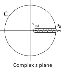
Figure 1: Cauchy’s Theorem on the $s$ plane

Then, if we introduce an arbitrary entire function $K\left(s\right)$ we can also write

$$\frac{1}{2\pi i}{\displaystyle\oint\limits_{\mathrm{C}}}K\left(s\right)\,\Pi^{\Gamma}\left(s\right)ds\,=\,0$$ (4)

Being $\Pi^{\Gamma}\left(s\right)$ real in the real axes outside the cut we can use Schwarz Reflection Principle and write:

$$\!\!\!\!\!\frac{1}{\pi}\int_{s_{\mathrm{cut}}}^{s_{0}}\!\!\!\!\!\!K\left(s\right)\,\mathrm{Im}\,\Pi^{\Gamma}\left(s\right)ds=\frac{-1}{2\pi i}\,\int_{\!\!\left|s\right|\,=\,s_{0}}\!\!\!\!\!\!K\left(s\right)\Pi^{\Gamma}\left(s\right)ds$$

In this relation we have split the contribution of the integral along the closed path $C$ into two parts (figure 1). In the l.h.s. the integration runs along the cut, including the low energy region starting at $s_{\mathrm{cut}}$, and in the r.h.s. the integral is performed along the circle of radius $s_{0}$ chosen in the high energy region. Along the cut we can use the experimental data information and in the circle we can calculate the correlator using asymptotic QCD. In this way we match theory with experiment.

The confrontation of theory and experiment by means of Cauchy’s Theorem yields what we call the finite energy sum rule

$$\frac{1}{\pi}\int_{s_{\mathrm{phys}}}^{s_{0}}K\left(s\right)\,\mathrm{Im}\,\Pi_{\mathrm{Data}}^{\Gamma}\left(s\right)ds\approx\,\!\!-\frac{1}{2\pi i}\int_{\left|s\right|=s_{0}}K\left(s\right)\,\Pi_{\mathrm{QCD}}^{\Gamma}\left(s\right)\,ds$$ (5)

where $s_{\mathrm{phys}}$ stands for the physical threshold.

Taking into account that the function $\Pi_{QCD}^{\Gamma}\left(s\right)$ has its own analytic structure, with a QCD cut in the real axes starting at $s_{QCD}$, we can substitute the r.h.s. of the former equation by an integral of the imaginary part along the cut, thus an equivalent relation is:

$$\frac{1}{\pi}\int_{s_{\mathrm{phys}}}^{s_{0}}K\left(s\right)\,\mathrm{Im}\,\Pi_{\mathrm{Data}}^{\Gamma}\left(s\right)\,ds\approx\,\frac{1}{\pi}\int_{s_{QCD}}^{s_{0}}K\left(s\right)\mathrm{Im}\Pi_{\mathrm{QCD}}^{\Gamma}\left(s\right)\,ds$$ (6)

Here we have to face the following problem. From the experimental data we usually know the physical spectrum near the physical threshold, where resonances appear, whereas at high energies we do not have information of the final multiparticle product spectrum. In order to match this information with the results of QCD at high energies we introduce a new parameter in the sum rule, that we call $s_{\mathrm{eff}}$, above which we are allowed for the substitution of experimental data by QCD in the physical cut.

1.3 The value of $s$ effective ($s_{\mathrm{eff}}$)

Let us define the effective threshold satisfying

$$\mathrm{Im}\,\Pi_{\mathrm{Data}}^{\Gamma}\left(s\right)\approx\mathrm{Im}\Pi_{\mathrm{QCD}}^{\Gamma}\left(s\right)\quad\mathrm{for}\,s\geqslant s_{\mathrm{eff}}$$ (7)

and

$$\frac{1}{\pi}\int_{s_{\mathrm{phys}}}^{s_{\mathrm{eff}}}K\left(s\right)\mathrm{Im}\,\Pi_{\mathrm{Data}}^{\Gamma}\left(s\right)ds\approx\frac{1}{\pi}\int_{s_{QCD}}^{s_{\mathrm{eff}}}K\left(s\right)\,\mathrm{Im}\,\Pi_{\mathrm{QCD}}^{\Gamma}\left(s\right)ds$$ (8)

This last relation does not follow from (6) just from the approximation of integrands (7). We need also to choose suitable “kernels” $K\left(s\right)$. As a result we face with two problems: how to choose the appropriate kernel and how to fix the value for $s_{\mathrm{eff}}$ to get a good approximation in equation (8).

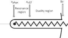
Figure 2: Physical cut

2 Choosing the appropriate Kernel

For sake of comparison we will focus our discussion in two kind of kernels: the exponential kernel and the Legendre Polynomial kernels, which are the object of this note.

2.1 Exponential Kernel: SVZ-Laplace Sum Rule

The exponential kernel, that was first introduced in [1], enhances the resonance region in the energy interval $\left[s_{\mathrm{phys}},s_{\mathrm{eff}}\right]$ and is given by

$$K\left(s,M^{2}\right)=e^{-s/M^{2}}$$

This falling down of the exponential kernel works in such a way that, on both the experimental data and the asymptotic QCD integrals, we can neglect the part of the integral in the interval $\left[s_{\mathrm{eff}},s_{0}\right]$ even in the limit $s_{0}\rightarrow\infty.$

Then, with this kernel the Sum Rule (8) becomes

$$\frac{1}{\pi}\int_{s_{\mathrm{phys}}}^{s_{\mathrm{eff}}}e^{-s/M^{2}}\,\mathrm{Im}\,\Pi_{\mathrm{Data}}^{\Gamma}\left(s\right)ds\approx\frac{1}{\pi}\int_{s_{QCD}}^{s_{\mathrm{eff}}}e^{-s/M^{2}}\,\mathrm{Im}\,\Pi_{\mathrm{QCD}}^{\Gamma}\left(s,m\right)ds$$ (9)

In the r.h.s. of (9) we have introduced a QCD mass parameter ($m$) to be estimated. The prediction of $m$ is done at some particular $M$ provided that there exists a neighbourhood of $M$ where this prediction is constant. Notice that $M$ fixes the slope of the exponential kernel in the resonance region, i.e. the amount of enhancement or suppression we introduce with the kernel.

2.2 Legendre Polynomial (LP) Kernels

This set of kernels, that was first successfully used in the calculation of the heavy quark masses [2, 3], is introduced defining a set of n-degree orthogonal polynomials $P_{n}(s)$ in the energy interval $s\,\in\,[s_{\mathrm{eff}},s_{0}]$ with a normalization condition at the lowest lying resonance, $s=M_{R}^{2}$, as follows:

$$\int_{s_{\mathrm{eff}}}^{s_{0}}s^{q}\,P_{n}(s)\,ds=0,~{}\ q=0,,1...,n-1$$

$$P_{n}(M_{R}^{2})=1$$ (10)

These polynomials are related to the ordinary Legendre polynomials $\mathcal{P}_{n}(x)$ in the interval $x\,\in\,[-1,1]$:

$$\!\!\!\!P_{n}(s)\,=\,\frac{\mathcal{P}_{n}\left(x(s)\right)}{\mathcal{P}_{n}\left(x(M_{R}^{2})\right)},\quad x(s)\,=\,\frac{2s\,-\,(s_{0}+s_{\mathrm{eff}})}{s_{0}-s_{\mathrm{eff}}}$$

We quote here some of the Legendre Polynomials we use:

$$\mathcal{P}_{2}\left(x\right) = \frac{1}{2}(3x^{2}-1),$$

$$\mathcal{P}_{3}\left(x\right) = \frac{1}{2}(5x^{3}-3x),$$

$$\mathcal{P}_{4}\left(x\right) = \frac{1}{8}(35x^{4}-30x^{2}+3),$$

$$\mathcal{P}_{5}\left(x\right) = \frac{1}{8}(63x^{5}-70x^{3}+15x).$$ (11)

Notice that the oscillatory nature of the polynomials cancels the unknown data in the interval $\left[s_{\mathrm{eff}},s_{0}\right]$ more efficiently than in the exponential case.

We quote here some of the Legendre Polynomials we use:

$$\frac{1}{\pi}\int_{s_{\mathrm{phys}}}^{s_{\mathrm{eff}}}P_{n}\left(s;s_{\mathrm{eff}},s_{0}\right)\,\mathrm{Im}\,\Pi_{\mathrm{Data}}^{\Gamma}\left(s\right)ds$$

$$\approx\frac{1}{\pi}\int_{s_{QCD}}^{s_{\mathrm{eff}}}P_{n}\left(s;s_{\mathrm{eff}},s_{0}\right)\,\mathrm{Im}\,\Pi_{\mathrm{QCD}}^{\Gamma}\left(s,m\right)ds$$ (12)

where $P_{n}\left(s;s_{\mathrm{eff}},s_{0}\right)$ are defined in the range $s\,\in\,\left[s_{\mathrm{eff}},s_{0}\right]$ according to (10).

Now the method to determine the QCD parameter $m$ within this sum rule works as follows:

• As a first step we study in equation (12) the stability of our prediction of $m$ with $s_{0},$ taking $s_{\mathrm{eff}}$ around the continuum physical threshold, beyond the resonance region.

• Then we adjust the value for $s_{\mathrm{eff}}$ by demanding optimal stability, namely that the function $m\left(s_{0}\right)$ remains constant in a plateau as large as possible.

• The estimate for $m$ is taken for the optimal stability values of the parameters $s_{0}$ and $s_{\mathrm{eff}}$.

• Finally, we check the convergence of the result with the degree of the polynomial ($n$).

To see how this sum rule method works in a particular calculation, we describe in the next section the determination of the $B$ decay constant ($f_{B}$).

3 Legendre Polynomial Kernel in the $f_{B}$ determination.

Taking the pseudoscalar correlator for the pair of quarks $ub$ and assuming the dominance of the lowest lying resonance ($B$ pole) we take:

$$\frac{1}{\pi}\,\mathrm{Im}\,\Pi_{\mathrm{Data}}^{\Gamma}\left(s\right)\,=\,f_{B}^{2}\,M_{B}^{4}\,\delta\left(s-M_{B}^{2}\right),$$ (13)

being the decay constant $f_{B}$ the unknown in equation (12):

$$\!\!\!\!\!\!\!\!\!\!\!f_{B}^{2}\left(s_{0}\right)\approx\frac{1}{\pi M_{B}^{4}}\int_{s_{QCD}}^{s_{\mathrm{eff}}}\!\!\!\!\!\!P_{n}\left(s;s_{\mathrm{eff}},s_{0}\right)\mathrm{Im}\,\Pi_{\mathrm{QCD}}^{\Gamma}\left(s\right)ds$$ (14)

The dependence of $f_{B}$ in $s_{0}$ is implicit in the definition of the polynomial $P_{n}\left(s;s_{\mathrm{eff}},s_{0}\right)$ (10). Choosing $s_{\mathrm{eff}}$ at the continuum physical threshold, $s_{\mathrm{eff}}=\left(M_{B}+2m_{\pi}\right)^{2}=29.9\,GeV^{2}$ as in [4, 5], the polynomials that give stable results for different degrees $n$ are depicted in figure 3.

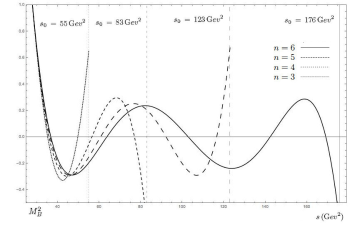
Figure 3: Legendre polynomials for $f_{B}$ with threshold $s_{phys}=29.9\,{\mathrm{G}ev}^{2}$ (see equation (11))

We see that the higher n we choose, the larger values for $s_{0}$ we need to find stability, however the slope of the polynomial remains roughly constant in the threshold region. Again we find, as in the exponential case, that the amount of enhancement of the resonance region is a fundamental issue in the sum rule method.

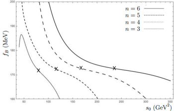
Figure 4: $f_{B}$ results for different polynomials at the physical threshold $s_{phys}=29.9\,{\mathrm{G}ev}^{2}$ (see text).

Also looking at the stability regions for different n degree of the LP kernel we appreciate in figure 4 that increasing the degree of the polynomial the plateau gets wider and the results, taken at the inflexion points, show a very good convergence with the polynomial degree, the result going to the value $f_{B}\sim 175\,\mathrm{Mev}$.

Next, instead of fixing $s_{\mathrm{eff}}$ at the continuum physical threshold, we determine it by demanding optimal stability [6]. In our case we will achieve this by imposing that the first derivative should also vanish at the inflexion point. Choosing this way to determine $s_{\mathrm{eff}}$ we improve substantially the stability region (as it is shown in figure 5) with a result for the decay constant slightly higher ($f_{B}\sim 186\,\mathrm{Mev}$) which is constant in a wider range of $s_{0}$. The value of optimal stability that we find for $s_{\mathrm{eff}}$ is not far from the physical continuum threshold, as one could anticipate, although the difference is crucial for stabilizing the result. This feature is one of the main motivations to trust the sum rule method with LP kernels.

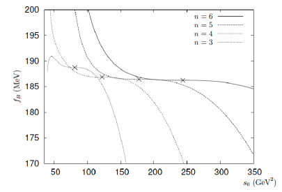
Figure 5: $f_{B}$ results for different polynomials at optimal $s_{eff}=31.3\,{\mathrm{G}ev}^{2}$ (see text).

A further advantage of this method is that the contribution of the sum rule integral in the region $\left[s_{\mathrm{eff}},s_{0}\right]$ is really tiny. As a matter of fact we have compared the QCD integration pieces in the $f_{B}$ calculation obtaining:

$$\frac{\int_{s_{\mathrm{eff}}}^{s_{0}}P_{n}\left(s;s_{\mathrm{eff}},s_{0}\right)\,\mathrm{Im}\Pi_{\mathrm{QCD}}^{\Gamma}\left(s,m\right)ds}{\int_{s_{QCD}}^{s_{\mathrm{eff}}}P_{n}\left(s;s_{\mathrm{eff}},s_{0}\right)\,\mathrm{Im}\Pi_{\mathrm{QCD}}^{\Gamma}\left(s,m\right)ds}\,\thicksim\,0.005$$

The same would happen in the experimental data integration provided we take $s_{\mathrm{eff}}$ beyond the resonance region. Obviously the lack of precise information introduces a systematic uncertainty of the method which is beyond our control. Nevertheless, we expect this uncertainty to be small, since even the resonances in the continuum region are substantially suppressed by the polynomials with respect to the lowest lying resonance (see figure 3).

4 Legendre Polynomial Kernel in the determination of the strange quark mass

The calculation of the light quark masses from the pseudoscalar current is a bit cumbersome due to the poor convergence of the QCD correlator with respect to the strong coupling. We give here some preliminary results using the LP sum rule method.

For the strange quark mass we use in the spectral function, aside from the Kaon pole, the contribution of the $K(1460)$ and $K(1830)$ resonances that significantly improves the convergence of the results. In order to perform the integration of the experimental side we use a Breit-Wigner model, as depicted in figure 6.

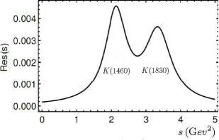
Figure 6: Resonance model in the Kaon channel (the kaon pole is omitted).

To have a flavour of the results obtained we present in figure 7 the stable values for the quark masses obtained with the 6th order Legendre polynomial. The stability regions of the mass with the value of $s_{0}$ is apparent, presenting again a nice plateau around the stability points. Results for different orders in the strong coupling constant show a fairly good convergence of the results for the masses. This convergence is worse than in the light-heavy quarks system calculations and further investigation is under way.

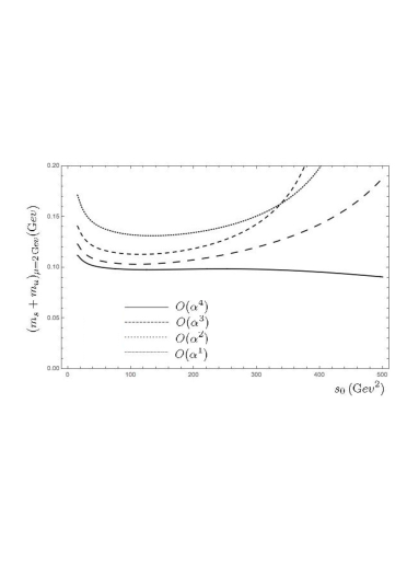
Figure 7: $m_{s}+m_{u}$ results at different orders of the strong coupling constant with a 5th degree polynomial ($s_{eff}=3.6\,{\mathrm{G}ev}^{2}$).

Aside from this consideration, what is important to stress here concerning the LP sum rule method, is that the value for $s_{\mathrm{eff}}$ is determined by optimal stability and it is located, as expected, just after the resonance region where one expects that the experimental results approach to some smooth function of the energy. On the other hand we have checked that the result has a very good convergence when the degree of the polynomial is increased.

5 Conclusions

To summarize, we have reviewed the main features of the FESR method with LP kernels. The main advantages that we find are:

• The LP kernels eliminate very efficiently the contribution of asymptotic QCD and the experimental data in the interval $\left[s_{\mathrm{eff}},s_{0}\right]$ of the Sum Rule integral.

• The LP kernels are easy to integrate with asymptotic QCD in the circle $\left|s\right|=s_{0}$ and one does not need to extract the imaginary part from the QCD correlator.

• The method is able to determine $s_{\mathrm{eff}}$ in a systematic way, which provides a better stability of the results (figure 5).

• The final results show nice plateaus with $s_{0}$ as well as a good convergence with the degree of the polynomial.

• The slope of the LP near the threshold approaches to a constant when increasing the degree of the polynomial.

• First used in the calculation of the heavy quark masses [2, 3] we have used it recently in the calculation of the meson decay constants in the heavy-light quark systems [4, 5, 6] and work in the pion and kaon channels is in progress [7].

References

- [1] M. A. Shifman, A. I. Vainshtein and V. I. Zakharov, Nucl. phys B 147 (1979) 448. Nucl. phys B 147 (1979) 385. Nucl. phys B 147 (1979) 519.
- [2] J. Penarrocha and K. Schilcher, phys Lett. B 515 (2001) 291.
- [3] J. Bordes, J. Penarrocha and K. Schilcher, phys Lett. B 562 (2003) 81.
- [4] J. Bordes, J. Penarrocha and K. Schilcher, JHEP 0412 (2004) 064.
- [5] J. Bordes, J. Penarrocha and K. Schilcher, JHEP 0511 (2005) 014.
- [6] M. J. Baker, J. Bordes, C. A. Dominguez, J. Penarrocha and K. Schilcher, JHEP 1407 (2014) 032
- [7] M. J. Baker, J. Bordes, C. A. Dominguez, J. Penarrocha and K. Schilcher, work in progress.