An Improved Composite Hypothesis Test for Markov Models with Applications in Network Anomaly Detection1

Abstract

Recent work has proposed the use of a composite hypothesis Hoeffding test for statistical anomaly detection. Setting an appropriate threshold for the test given a desired false alarm probability involves approximating the false alarm probability. To that end, a large deviations asymptotic is typically used which, however, often results in an inaccurate setting of the threshold, especially for relatively small sample sizes. This, in turn, results in an anomaly detection test that does not control well for false alarms. In this paper, we develop a tighter approximation using the Central Limit Theorem (CLT) under Markovian assumptions. We apply our result to a network anomaly detection application and demonstrate its advantages over earlier work.

I Introduction

During the last decade, the applications of statistical anomaly detection in communication networks using the Large Deviations Theory (LDT) [1] have been extensively explored; see, e.g., [2], [3], [4], among others. Statistical anomaly detection involves characterizing the “normal behavior” of the system and identifying the time instances corresponding to abnormal system behavior. Assuming that the network traffic is stationary in time, [2] applies two methods to that end. The first method, termed “model-free,” models traffic as an independent and identically distributed (i.i.d.) sequence. The second method, termed “model-based,” models traffic as a finite-state Markov chain. These are then extended in [4] to the case where the network traffic is time-varying. Essentially, each of these methods is designed to tackle a certain Universal Hypothesis Testing Problem (UHTP).

A UHTP aims to test the hypothesis that a given sequence of observations is drawn from a known Probability Law (PL) (i.e., probability distribution) defined on a finite alphabet [5]. It is well known that the test proposed by Hoeffding [6] is optimal in an error exponent sense [1], [2], [4]. When implementing Hoeffding’s test, one must set a threshold $\eta$, which can be estimated by using Sanov’s theorem [1], a result within the scope of LDT. Note that such an estimate (let us denote it by $\eta^{sv}$) is valid only in the asymptotic sense. In practice, however, only a finite number of observations are available, and it can be shown by experiments (e.g., using the software package TAHTIID [7]) that $\eta^{sv}$ is typically not accurate enough.

To improve the accuracy of the estimation for $\eta$, [5] (or, see [8]) borrows a method typically used by statisticians; that is, deriving results based on Weak Convergence (WC) of the test statistic to approximate the error probabilities of Hoeffding’s test. Under the i.i.d. assumption, by using the technique combining WC results together with Taylor’s series expansion, [5] (or, see [8], [9]) gives an alternative approximation for $\eta$ (let us denote it by $\eta^{wc}$). Using [7], one can verify that, in the finite sample-size setting, $\eta^{wc}$ is typically much more accurate than $\eta^{sv}$.

It is worth pointing out that some researchers have also tried to obtain a more accurate approximation for $\eta$ by refining Sanov’s theorem [10]. However, as noted in [8], such refinements of large deviation results are typically hard to calculate.

In this work we establish $\eta^{wc}$ under a Markovian assumption, thus, extending the work of [5] which considered the i.i.d. case. We apply the proposed procedure to network anomaly detection by embedding it into the software package SADIT [11].

The rest of the paper is organized as follows. We first formulate the problem in Sec. II and derive the theoretical results in Sec. III. We then present the experimental results in Sec. IV and finally provide concluding remarks in Sec. V.

Notation: By convention, all vectors are column vectors. To save space, we write ${\mathbf{x}}=(x_{1},\ldots,x_{n})$ to denote the column vector ${\mathbf{x}}$. We use prime to denote the transpose of a matrix or vector.

II Problem Formulation

Let $\Xi=\left\{{\xi_{i}};~{}i=1,\ldots,N\right\}$ be a finite alphabet. The observations ${\mathbf{Y}}=\left\{{{Y_{l}};~{}l=0,1,2,\ldots}\right\}$ form a stochastic process taking values from $\Xi$.

In the model-based UHTP [1], [2], [4], under the null hypothesis $\cal H$, the observations ${\mathbf{Y}}=\left\{{{Y_{l}};~{}l=0,1,2,\ldots}\right\}$ are drawn according to a Markov chain with state set $\Xi$. Let its transition matrix be ${\mathbf{Q}}=\left({{q_{ij}}}\right)_{i,j=1}^{N}$.

Let $\textbf{1}_{\{\cdot\}}$ denote the indicator function. Define the empirical PL by

$${\Gamma_{n}}\left({{\theta_{ij}}}\right)=\frac{1}{n}\sum\nolimits_{l=1}^{n}{\textbf{1}_{\left\{{{Z_{l}}={\theta_{ij}}}\right\}}},$$ (1)

where ${Z_{l}}=\left({{Y_{l-1}},~{}{Y_{l}}}\right),~{}l=1,\ldots,n$, ${\theta_{ij}}=\left({{\xi_{i}},~{}{\xi_{j}}}\right)\in\Xi\times\Xi$, $i,j=1,\ldots,N$, and denote the new alphabet $\Theta=\left\{{{\theta_{ij}}};~{}i,j=1,\ldots,N\right\}=\left\{{{{\tilde{\theta}}_{k}}};~{}k=1,\ldots,N^{2}\right\}$. Note that $\Theta=\Xi\times\Xi$ and ${{\tilde{\theta}}_{1}}={\theta_{11}}$, $\ldots$, ${{\tilde{\theta}}_{N}}={\theta_{1N}}$, $\ldots$, ${{\tilde{\theta}}_{\left({N-1}\right)N+1}}={\theta_{N1}}$, $\ldots$, ${{\tilde{\theta}}_{{N^{2}}}}={\theta_{NN}}$. Let also the set of PLs on $\Theta$ be $\mathcal{P}(\Theta)$.

It is seen that the transformed observations ${\mathbf{Z}}=\left\{{{Z_{l}};~{}l=1,2,\ldots}\right\}$ form a Markov chain evolving on $\Theta$. Let its transition matrix be ${\mathbf{P}}=\left({{p_{ij}}}\right)_{i,j=1}^{{N^{2}}}$ with stationary distribution

$${\bm{\pi}}=\left({{\pi_{ij}}};~{}i,j=1,\ldots,N\right)=\left({{{\tilde{\pi}}_{k}}};~{}k=1,\ldots,N^{2}\right),$$

where ${{\pi_{ij}}}$ denotes the probability of seeing $\theta_{ij}$, and ${{\tilde{\pi}}_{1}}={{\pi}_{11}}$, $\ldots$, ${{\tilde{\pi}}_{N}}={{\pi}_{1N}}$, $\ldots$, ${{\tilde{\pi}}_{\left({N-1}\right)N+1}}={{\pi}_{N1}}$, $\ldots$, ${{\tilde{\pi}}_{{N^{2}}}}={{\pi}_{NN}}$. Let $p\left({{\theta_{ij}}\left|{{\theta_{kl}}}\right.}\right)$ denote the transition probability from $\theta_{kl}$ to $\theta_{ij}$. Then we have

$$p\left({{\theta_{ij}}\left|{{\theta_{kl}}}\right.}\right)=\textbf{1}_{\left\{{i=l}\right\}}{q_{ij}},\quad k,l,i,j=1,\ldots,N,$$

which enables us to obtain ${\mathbf{P}}$ directly from ${\mathbf{Q}}$.

Write ${\bm{\pi}}=({{\pi_{11}}},\ldots,{{\pi_{1N}}},\ldots,{{\pi_{N1}}},\ldots,{{\pi_{NN}}})$, and ${\bm{\Gamma}_{n}}=({{\Gamma_{n}}\left({{\theta_{11}}}\right)},\ldots,{{\Gamma_{n}}\left({{\theta_{1N}}}\right)},\ldots,{{\Gamma_{n}}\left({{\theta_{N1}}}\right)},\ldots,{{\Gamma_{n}}\left({{\theta_{NN}}}\right)})$.

Define the relative entropy (i.e., divergence)

$$D\left({\left.{{\bm{\Gamma}_{n}}}\right\|\bm{\pi}}\right)=\sum\limits_{i=1}^{N}{\sum\limits_{j=1}^{N}{{\Gamma_{n}}\left({{\theta_{ij}}}\right)\log\frac{{{{{\Gamma_{n}}\left({{\theta_{ij}}}\right)}\mathord{\left/{\vphantom{{{\Gamma_{n}}\left({{\theta_{ij}}}\right)}{\sum\nolimits_{j=1}^{N}{{\Gamma_{n}}\left({{\theta_{ij}}}\right)}}}}\right.\kern-1.2pt}{{\sum\nolimits_{j=1}^{N}{{\Gamma_{n}}\left({{\theta_{ij}}}\right)}}}}}}{{{{{\pi_{ij}}}\mathord{\left/{\vphantom{{{\pi_{ij}}}{{\sum\nolimits_{j=1}^{N}{{\pi_{ij}}}}}}}\right.\kern-1.2pt}{{\sum\nolimits_{j=1}^{N}{{\pi_{ij}}}}}}}}}},$$ (2)

and the empirical measure

$${{\mathbf{U}}_{n}}=\sqrt{n}\left({{\bm{\Gamma}_{n}}-\bm{\pi}}\right).$$ (3)

For any positive integer $n$, let ${{\cal{H}}_{n}}$ be the output of the test that decides to accept or to reject the null hypothesis $\cal H$ based on the first $n$ observations in the sequence ${\mathbf{Z}}$. Under the Markovian assumption, Hoeffding’s test [1] is given by

$${{\cal{H}}_{n}}={\cal{H}}\Leftrightarrow D\left({\left.{{\bm{\Gamma}_{n}}}\right\|{\bm{\pi}}}\right)\leq\eta_{n},$$ (4)

where $D\left({\left.{{\bm{\Gamma}_{n}}}\right\|{\bm{\pi}}}\right)$, defined in (2), is the test statistic, and $\eta_{n}$ is a threshold. Note that, when applied in anomaly detection, Hoeffding’s test will report an anomaly if and only if ${{\cal{H}}_{n}}\neq\cal H$, or, equivalently, $D\left({\left.{{\bm{\Gamma}_{n}}}\right\|{\bm{\pi}}}\right)>\eta_{n}$.

Under hypothesis $\cal H$, the false alarm probability [5] of the test sequence $\left\{{{{\cal H}_{n}}}\right\}$ as a function of $n$ is defined by

$${\beta_{n}}={P_{\cal H}}\left\{{D\left({\left.{{\bm{\Gamma}_{n}}}\right\|{\bm{\pi}}}\right)>\eta_{n}}\right\},$$ (5)

where $P_{\cal H}\{A\}$ denotes the probability of event $A$ under hypothesis $\cal H$. Sanov’s theorem [1] implies the approximation for $\eta_{n}$

$$\eta_{n}^{sv}\approx-\frac{1}{n}\log\left({{\beta_{n}}}\right).$$ (6)

Given $\beta_{n}\in(0,1)$, our central goal in this paper is to improve the accuracy of the approximation for $\eta_{n}$.

III Theoretical Results

We introduce the following condition:

Condition (C). ${\mathbf{Z}}=\left\{{{Z_{l}};~{}l=1,2,\ldots}\right\}$ is an aperiodic, irreducible, and positive recurrent Markov chain [12], [13] evolving on $\Theta$ with stationary distribution $\bm{\pi}$, and with the same $\bm{\pi}$ as its initial distribution.

Remark 1: Since $\Theta$ is a finite set, we know that ${\mathbf{Z}}$ is uniformly ergodic [12], [14]. Assuming the initial distribution to be $\bm{\pi}$ is for notational simplicity; our results apply for any feasible initial distribution. Note also that, under (C), $\bm{\pi}$ must have full support over $\Theta$, meaning each entry in $\bm{\pi}$ is strictly positive.

Lemma III.1

Assume (C) holds. Then

$$\frac{{{\pi_{ij}}}}{{\sum\nolimits_{t=1}^{N}{{\pi_{it}}}}}=\frac{{{\pi_{ij}}}}{{\sum\nolimits_{t=1}^{N}{{\pi_{ti}}}}}={q_{ij}},\quad i,j=1,\ldots,N.$$ (7)

Proof.

Expanding the first $N$ entries of $\bm{\pi}{\mathbf{P}}=\bm{\pi}$, we obtain $q_{1i}\sum\nolimits_{t=1}^{N}{{\pi_{t1}}}={\pi_{1i}},~{}i=1,\ldots,N$. Summing up both sides of these equations, it follows

$$\left({\sum\nolimits_{i=1}^{N}{{q_{1i}}}}\right)\cdot\sum\nolimits_{t=1}^{N}{{\pi_{t1}}}=\sum\nolimits_{t=1}^{N}{{\pi_{1t}}}.$$ (8)

Noticing $\sum\nolimits_{i=1}^{N}{{q_{1i}}}=1$, we see that (8) implies $\sum\nolimits_{t=1}^{N}{{\pi_{t1}}}=\sum\nolimits_{t=1}^{N}{{\pi_{1t}}}$, which, together with $q_{11}\sum\nolimits_{t=1}^{N}{{\pi_{t1}}}={\pi_{11}}$, yields

$$\frac{{{\pi_{11}}}}{{\sum\nolimits_{t=1}^{N}{{\pi_{1t}}}}}=\frac{{{\pi_{11}}}}{{\sum\nolimits_{t=1}^{N}{{\pi_{t1}}}}}={q_{11}}.$$

Similarly, we can show (7) holds for all the other $(i,j)$’s. ∎

Remark 2: By Remark 1 and Lemma III.1 we see that, under Condition (C), all entries in ${\mathbf{Q}}$ are strictly positive, indicating that any two states of the original chain ${\mathbf{Y}}$ are connected. This is a strict condition; yet, in engineering practice, if some $\pi_{ij}$ in (7) are equal to zero, we can always replace them with a small positive value, and then normalize the modified vector $\bm{\pi}$, thus ensuring that Condition (C) can be satisfied. See Sec. IV-A for an illustration of this trick.

III-A Weak convergence of ${\mathbf{U}}_{n}$

Let us first establish CLT results for one-dimensional empirical measures

$$U_{n}^{\scriptscriptstyle{\left(k\right)}}=\sqrt{n}\left({{\Gamma_{n}}\left({{{\tilde{\theta}}_{k}}}\right)-{{\tilde{\pi}}_{k}}}\right),\quad k=1,\ldots,{N^{2}}.$$ (9)

Fix $k\in\{1,\ldots,N^{2}\}$. Define

$${f_{k}}\left(Z\right)=\textbf{1}_{\left\{{Z={{\tilde{\theta}}_{k}}}\right\}}=\left\{\begin{gathered}1,{\text{ if }}Z={{\tilde{\theta}}_{k}},\hfill\\ 0,{\text{ if }}Z\in\Theta\backslash\left\{{{{\tilde{\theta}}_{k}}}\right\}.\hfill\\ \end{gathered}\right.$$ (13)

Lemma III.2

Assume (C) holds. Then a CLT holds for $U_{n}^{\scriptscriptstyle{\left(k\right)}}$; that is, $U_{n}^{\scriptscriptstyle{\left(k\right)}}\xrightarrow[n\to\infty]{{d.}}\mathcal{N}\left({0,~{}\sigma_{k}^{2}}\right)$ with $\sigma_{k}^{2}=\operatorname{Cov}\left({{f_{k}}\left({{Z_{1}}}\right),~{}{f_{k}}\left({{Z_{1}}}\right)}\right)+2\sum\nolimits_{m=1}^{\infty}{\operatorname{Cov}}\left({{f_{k}}\left({{Z_{1}}}\right),~{}{f_{k}}\left({{Z_{1+m}}}\right)}\right)<\infty$.

Proof.

This can be established by applying [12, Corollary 1]. Noting $f_{k}(\cdot)$ is bounded and the chain ${\mathbf{Z}}$ is uniformly ergodic, we see that all the conditions needed by [12, Corollary 1] are satisfied. ∎

Now we can directly extend Lemma III.2 to the multidimensional case (for an informal argument, see, e.g., [15]; cf. [16, Sec. iii@.6] for the definition of a Gaussian random variable with a general normal distribution). Due to its role in the following applications, we state the result as a theorem.

Theorem III.3

Assume (C) holds. Then a multidimensional CLT holds for ${\mathbf{U}}_{n}$; that is,

$${{\mathbf{U}}_{n}}\xrightarrow[n\to\infty]{{d.}}\mathcal{N}\left({0,~{}\bm{\Lambda}}\right)$$ (14)

with $\bm{\Lambda}$ being an $N^{2}\times N^{2}$ covariance matrix given by

$$\bm{\Lambda}={\bm{\Lambda}_{0}}+\sum\nolimits_{m=1}^{\infty}{{\bm{\Lambda}_{m}}},$$ (15)

where ${\bm{\Lambda}_{0}}$ and ${\bm{\Lambda}_{m}}$ are specified, respectively, by ${\bm{\Lambda}_{0}}=\left[{\operatorname{Cov}\left({{f_{i}}\left({{Z_{1}}}\right),~{}{f_{j}}\left({{Z_{1}}}\right)}\right)}\right]_{i,j=1}^{{N^{2}}}$ and ${\bm{\Lambda}_{m}}=\left[{{{\operatorname{Cov}}}\left({{f_{i}}\left({{Z_{1}}}\right),~{}{f_{j}}\left({{Z_{1+m}}}\right)}\right)+{{\operatorname{Cov}}}\left({{f_{j}}\left({{Z_{1}}}\right),~{}{f_{i}}\left({{Z_{1+m}}}\right)}\right)}\right]_{i,j=1}^{{N^{2}}}$, $m=1,2,\ldots$.

The rest of this subsection is devoted to the computation of $\bm{\Lambda}$; we will express $\bm{\Lambda}=\big{[}{{\Lambda^{\scriptscriptstyle{\left({i,j}\right)}}}}\big{]}_{i,j=1}^{{N^{2}}}$ in terms of the quantities determining the probabilistic structure of the chain ${\mathbf{Z}}$.

In particular, we have

$$\Lambda_{0}^{\scriptscriptstyle{\left({i,j}\right)}}={\text{Cov}}\big{(}{\textbf{1}_{\{{{Z_{1}}={{\tilde{\theta}}_{i}}}\}},~{}\textbf{1}_{\{{{Z_{1}}={{\tilde{\theta}}_{j}}}\}}}\big{)},\quad i,j=1,\ldots,{N^{2}},$$ (16)

and

$$\Lambda_{m}^{\scriptscriptstyle{\left({i,j}\right)}}~{}=~{} {\text{Cov}}\big{(}{\textbf{1}_{\{{{Z_{1}}={{\tilde{\theta}}_{i}}}\}},~{}\textbf{1}_{\{{{Z_{1+m}}={{\tilde{\theta}}_{j}}}\}}}\big{)}$$

$$+{\text{Cov}}\big{(}{\textbf{1}_{\{{{Z_{1}}={{\tilde{\theta}}_{j}}}\}},~{}\textbf{1}_{\{{{Z_{1+m}}={{\tilde{\theta}}_{i}}}\}}}\big{)},$$ (17)

$m=1,2,\ldots;~{}i,j=1,\ldots,{N^{2}}$.

We first determine (16) as follows. By direct calculation, we obtain $\Lambda_{0}^{\scriptscriptstyle{\left({1,1}\right)}}={{\tilde{\pi}}_{1}}\left({1-{{\tilde{\pi}}_{1}}}\right)$, $\Lambda_{0}^{\scriptscriptstyle{\left({1,2}\right)}}=-{{\tilde{\pi}}_{1}}{{\tilde{\pi}}_{2}}$, and so on. In general, we have $\Lambda_{0}^{\scriptscriptstyle{\left({i,j}\right)}}=\tilde{\pi}_{i}\left({\mathbf{I}}_{ij}-\tilde{\pi}_{j}\right),~{}i,j=1,\ldots,{N^{2}}$, where ${\mathbf{I}}_{ij}$ denotes the $(i,j)$-th entry of the identity matrix.

Now we compute $\Lambda_{2}^{\scriptscriptstyle{\left({i,j}\right)}}$ by (17). Omitting the details, again by direct calculation, we arrive at ${\text{Cov}}\big{(}{\textbf{1}_{\{{{Z_{1}}={{\tilde{\theta}}_{i}}}\}},\textbf{1}_{\{{{Z_{3}}={{\tilde{\theta}}_{j}}}\}}}\big{)}={{\tilde{\pi}}_{i}}\big{(}{{{\mathbf{P}}^{2}_{ij}}-{{\tilde{\pi}}_{j}}}\big{)}$, where ${\mathbf{P}}^{2}_{ij}$ is the $(i,j)$-th entry of the matrix ${\mathbf{P}}^{2}$ (the square of the transition matrix ${\mathbf{P}}$). Interchanging the indexes $i,j$, we obtain ${\text{Cov}}\big{(}{\textbf{1}_{\{{{Z_{1}}={{\tilde{\theta}}_{j}}}\}},\textbf{1}_{\{{{Z_{3}}={{\tilde{\theta}}_{i}}}\}}}\big{)}=\tilde{\pi}_{j}\big{(}{\mathbf{P}}^{2}_{ji}-\tilde{\pi}_{i}\big{)}$. Thus, we have $\Lambda_{2}^{\scriptscriptstyle{\left({i,j}\right)}}={{\tilde{\pi}}_{i}}\big{(}{\mathbf{P}}_{ij}^{2}-\tilde{\pi}_{j}\big{)}+{{\tilde{\pi}}_{j}}\big{(}{\mathbf{P}}_{ji}^{2}-\tilde{\pi}_{i}\big{)}$.

Computing in a similar way, in general, we derive

$$\Lambda_{m}^{\scriptscriptstyle{\left({i,j}\right)}}={{\tilde{\pi}}_{i}}\left({{\mathbf{P}}_{ij}^{m}-{{\tilde{\pi}}_{j}}}\right)+{{\tilde{\pi}}_{j}}\left({{\mathbf{P}}_{ji}^{m}-{{\tilde{\pi}}_{i}}}\right),\quad m=1,2,\ldots,$$

where ${\mathbf{P}}^{m}_{ij}$ is the $(i,j)$-th entry of the matrix ${\mathbf{P}}^{m}$ (the $m$-th power of the transition matrix ${\mathbf{P}}$).

Thus, for $i,j=1,\ldots,{N^{2}}$ we finally attain

$${\Lambda^{\scriptscriptstyle{\left({i,j}\right)}}}={{\tilde{\pi}}_{i}}\left({{{\mathbf{I}}_{ij}}-{{\tilde{\pi}}_{j}}}\right)+\sum\nolimits_{m=1}^{\infty}{\left[{{\tilde{\pi}}_{i}}\left({{\mathbf{P}}_{ij}^{m}-{{\tilde{\pi}}_{j}}}\right)+{{\tilde{\pi}}_{j}}\left({\mathbf{P}}_{ji}^{m}-\tilde{\pi}_{i}\right)\right]}.$$ (18)

III-B Taylor’s series expansion of ${D}\left({{\bm{\Gamma}_{n}}\left\|{{\bm{\pi}}}\right.}\right)$

Inspired by [5] (or, see [8]) wherein the i.i.d. assumption is required, we use a Taylor’s series expansion to approximate the relative entropy ${D}\left({{\bm{\Gamma}_{n}}\left\|{{\bm{\pi}}}\right.}\right)$.

To this end, for $\bm{\nu}\in\mathcal{P}\left(\Theta\right)$ let us consider

$$h\left(\bm{\nu}\right)={D}\left({\bm{\nu}\left\|\bm{\pi}\right.}\right)=\sum\limits_{i=1}^{N}{\sum\limits_{j=1}^{N}{{\nu_{ij}}\log\frac{{\frac{{{\nu_{ij}}}}{{\sum\nolimits_{t=1}^{N}{{\nu_{it}}}}}}}{{\frac{{{\pi_{ij}}}}{{\sum\nolimits_{t=1}^{N}{{\pi_{it}}}}}}}}}.$$ (19)

By direct calculation, we derive

$$\frac{{\partial h\left({\bm{\nu}}\right)}}{{\partial{\nu_{ij}}}}= \log{\nu_{ij}}-\log\left({\sum\nolimits_{t=1}^{N}{{\nu_{it}}}}\right)-\log{\pi_{ij}}$$

$$+\log\left({\sum\nolimits_{t=1}^{N}{{\pi_{it}}}}\right),\quad i,j=1,\ldots,N,$$ (20)

which leads to

$$\nabla h\left(\bm{\pi}\right)=0.$$ (21)

Further, from (20), we compute the Hessian ${\nabla^{2}}h\left(\bm{\nu}\right)$ by considering three cases:

(i) If $k\neq i$, then $\frac{{{\partial^{2}}h\left(\bm{\nu}\right)}}{{\partial{\nu_{ij}}\partial{\nu_{kl}}}}=0$.

(ii) If $k=i$ and $l=j$, then

$$\frac{{{\partial^{2}}h\left(\bm{\nu}\right)}}{{\partial{\nu_{ij}}\partial{\nu_{kl}}}}=\frac{{{\partial^{2}}h\left(\bm{\nu}\right)}}{{\partial\nu_{ij}^{2}}}=\frac{1}{{{\nu_{ij}}}}-\frac{1}{{\sum\nolimits_{j=1}^{N}{{\nu_{ij}}}}}.$$

(iii) If $k=i$ and $l\neq j$, then

$$\frac{{{\partial^{2}}h\left(\bm{\nu}\right)}}{{\partial{\nu_{ij}}\partial{\nu_{kl}}}}=\frac{{{\partial^{2}}h\left(\bm{\nu}\right)}}{{\partial{\nu_{ij}}\partial{\nu_{il}}}}=-\frac{1}{{\sum\nolimits_{j=1}^{N}{{\nu_{ij}}}}}.$$

All these terms evaluated at $\bm{\pi}$ yield ${\nabla^{2}}h\left(\bm{\pi}\right)$, which will play a crucial role in approximating ${D}\left({{\bm{\Gamma}_{n}}\left\|{{\bm{\pi}}}\right.}\right)$.

From the ergodicity of the chain ${\mathbf{Z}}$, it follows ${\bm{\Gamma}_{n}}\xrightarrow[n\to\infty]{{a.s.}}\bm{\pi}$. It is seen that both $\nabla h\left(\bm{\nu}\right)$ and ${\nabla^{2}}h\left(\bm{\nu}\right)$ are continuous in a neighborhood of $\bm{\pi}$, and we can use the second-order Taylor’s series expansion of $h\left(\bm{\nu}\right)$ centered at $\bm{\pi}$ to approximate ${D}\left({{\bm{\Gamma}_{n}}\left\|{{\bm{\pi}}}\right.}\right)=h(\bm{\Gamma}_{n})-h\left(\bm{\pi}\right)$. To be specific, we have

$${D}\left({{\bm{\Gamma}_{n}}\left\|\bm{\pi}\right.}\right)\approx\frac{1}{2}{\left({{\bm{\Gamma}_{n}}-\bm{\pi}}\right)^{\prime}}{\nabla^{2}}h\left(\bm{\pi}\right)\left({{\bm{\Gamma}_{n}}-\bm{\pi}}\right).$$ (22)

III-C Threshold approximation

We use an empirical CDF to approximate the actual CDF of $D\left({\left.{{\bm{\Gamma}_{n}}}\right\|{\bm{\pi}}}\right)$. In particular, by (22) we have

$${D}\left({{\bm{\Gamma}_{n}}\left\|\bm{\pi}\right.}\right)\approx\frac{1}{{2n}}{\left({\sqrt{n}\left({{\bm{\Gamma}_{n}}-\bm{\pi}}\right)}\right)^{\prime}}{\nabla^{2}}h\left(\bm{\pi}\right)\left({\sqrt{n}\left({{\bm{\Gamma}_{n}}-\bm{\pi}}\right)}\right),$$ (23)

where, by Thm. III.3, $\sqrt{n}\left({{\bm{\Gamma}_{n}}-\bm{\pi}}\right)\xrightarrow[n\to\infty]{{d.}}\mathcal{N}\left({0,~{}\bm{\Lambda}}\right)$ with $\bm{\Lambda}$ given by (18). Thus, to derive an empirical CDF, we can generate a set of Gaussian sample vectors independently according to $\mathcal{N}\left({0,~{}\bm{\Lambda}}\right)$ and then plug each such sample vector into (23) (i.e., replace $\sqrt{n}\left({{\bm{\Gamma}_{n}}-\bm{\pi}}\right)$) and compute the right hand side of (23), thus, obtaining a set of sample scalars, as an approximation for samples of ${D}\left({{\bm{\Gamma}_{n}}\left\|\bm{\pi}\right.}\right)$.

Once we obtain an empirical CDF of ${D}\left({{\bm{\Gamma}_{n}}\left\|\bm{\pi}\right.}\right)$, say, denoted ${F_{em}}\left(\cdot;~{}n\right)$, then, by (5), we can use it to estimate $\eta_{n}$ as

$$\eta_{n}^{wc}\approx F_{em}^{-1}\left({1-{\beta_{n}}};~{}n\right),$$ (24)

where $F_{em}^{-1}(\cdot;~{}n)$ is the inverse of $F_{em}(\cdot;~{}n)$.

Clearly, to calculate the right hand side of (23), we need the parameter $\bm{\pi}$. In practice, we typically do not know the actual values of the underlying chain parameters, so we need to estimate them accordingly. This can be done by computing $\bm{\Gamma}_{n}$ over a long past sample path.

IV Experimental Results

IV-A Numerical results for threshold approximation

The experiments in this subsection are performed using the software package TAHTMA [17]. For convenience, we use $\Theta=\{1,2,\ldots,N^{2}\}$ to indicate the states, and assume $\bm{\pi}$ (ground truth) is the initial distribution.

In the following numerical examples, we first randomly create a valid (i.e., such that (C) holds) $N\times N$ transition matrix ${\mathbf{Q}}$, hence an $N^{2}\times N^{2}$ transition matrix ${\mathbf{P}}$, and then generate $T$ samples of the chain ${\mathbf{Z}}$, each with length $n$, denoted ${{\mathbf{Z}}^{\scriptscriptstyle{\left(t\right)}}}=\big{\{}{Z_{1}^{\scriptscriptstyle{\left(t\right)}},\ldots,Z_{n}^{\scriptscriptstyle{\left(t\right)}}}\big{\}},~{}t=1,\ldots,T$. These samples will be used to derive empirical CDF’s. Also, to estimate the parameters of interest, we generate one more training sample ${{\mathbf{Z}}^{\scriptscriptstyle{\left(0\right)}}}=\big{\{}{Z_{1}^{\scriptscriptstyle{\left(0\right)}},\ldots,Z_{n_{0}}^{\scriptscriptstyle{\left(0\right)}}}\big{\}}$, where $n_{0}$ is the length. The stationary distribution $\bm{\pi}$ (estimation) of the chain is computed by taking any row of ${\mathbf{P}}^{m_{0}}$, where $m_{0}$ is a sufficiently large integer.

With samples ${{\mathbf{Z}}^{\scriptscriptstyle{\left(t\right)}}}=\big{\{}{Z_{1}^{\scriptscriptstyle{\left(t\right)}},\ldots,Z_{n}^{\scriptscriptstyle{\left(t\right)}}}\big{\}},~{}t=1,\ldots,T$, we can compute $T$ samples of the scalar random variable ${D}\left({{\bm{\Gamma}_{n}}\left\|{{\bm{\pi}}}\right.}\right)$, by (2). Thus, an empirical CDF of ${D}\left({{\bm{\Gamma}_{n}}\left\|{{\bm{\pi}}}\right.}\right)$, denoted ${F}\left(\cdot;~{}n\right)$, can be derived. We will treat ${F}\left(\cdot;~{}n\right)$ as the actual CDF of ${D}\left({{\bm{\Gamma}_{n}}\left\|{{\bm{\pi}}}\right.}\right)$. The threshold given by (24) with ${F}\left(\cdot;~{}n\right)$ (i.e., $F(\cdot;~{}n)$ plays the role of $F_{em}(\cdot;~{}n)$) is then taken as the theoretical (actual) value $\eta_{n}$.

Next we derive an estimated empirical CDF of ${D}\left({{\bm{\Gamma}_{n}}\left\|{{\bm{\pi}}}\right.}\right)$, using Taylor’s series expansion together with Thm. III.3.

Let us first estimate the parameters of interest. Recall ${\bm{\pi}}=\left({{\pi_{ij}}};~{}i,j=1,\ldots,N\right)=\left({{{\tilde{\pi}}_{k}}};~{}k=1,\ldots,N^{2}\right)$. We estimate ${{{\tilde{\pi}}_{k}}}$ by

$${{\hat{\tilde{\pi}}}_{k}}=\max\left\{{\frac{{\sum\nolimits_{i=1}^{{n_{0}}}{\textbf{1}_{\big{\{}{Z_{i}^{\scriptscriptstyle{\left(0\right)}}=k}\big{\}}}}}}{{{n_{0}}}},~{}\varepsilon}\right\},\quad k=1,\ldots,N^{2},$$ (25)

where $\varepsilon>0$ is a small number. The purpose of introducing $\varepsilon$ is to avoid division by zero. Then, we obtain an estimated $\bm{\pi}$ as $\hat{\bm{\pi}}=\big{(}{{{{{\hat{\tilde{\pi}}}_{k}}}}\mathord{\left/{\vphantom{12}}\right.\kern-1.2pt}{{\sum\nolimits_{j=1}^{{N^{2}}}{{{\hat{\tilde{\pi}}}_{j}}}}}};~{}k=1,\ldots,N^{2}\big{)}$, or written $\hat{\bm{\pi}}=\left({{{\hat{\pi}}_{ij}}};~{}i,j=1,\ldots,N\right)$, where ${{\hat{\pi}}_{11}}={{{\hat{\tilde{\pi}}}_{1}}}\mathord{\left/{\vphantom{12}}\right.\kern-1.2pt}{{\hat{s}}}$, $\ldots$, ${{\hat{\pi}}_{1N}}={{{{\hat{\tilde{\pi}}}_{N}}}}\mathord{\left/{\vphantom{12}}\right.\kern-1.2pt}{{\hat{s}}}$, $\ldots$, ${{\hat{\pi}}_{N1}}={{{{\hat{\tilde{\pi}}}_{\left({N-1}\right)N+1}}}}\mathord{\left/{\vphantom{12}}\right.\kern-1.2pt}{{\hat{s}}}$, $\ldots$, ${{\hat{\pi}}_{NN}}={{{{\hat{\tilde{\pi}}}_{{N^{2}}}}}}\mathord{\left/{\vphantom{12}}\right.\kern-1.2pt}{{\hat{s}}}$, with $\hat{s}=\sum\nolimits_{j=1}^{{N^{2}}}{{{\hat{\tilde{\pi}}}_{j}}}$ being the normalization constant.

We are now ready to calculate the estimate for ${\nabla^{2}}\left(\boldsymbol{\pi}\right)$, by evaluating ${\nabla^{2}}\left(\hat{\boldsymbol{\pi}}\right)$.

Further, by Lemma III.1, we estimate ${\mathbf{Q}}$ by

$${{\hat{q}}_{ij}}=\frac{{{{\hat{\pi}}_{ij}}}}{{\sum\nolimits_{t=1}^{N}{{{\hat{\pi}}_{it}}}}},\quad i,j=1,\ldots,N.$$ (26)

Then an estimation of ${\mathbf{P}}$, denoted $\hat{{\mathbf{P}}}$, can be directly derived from $\hat{{\mathbf{Q}}}$.

Finally, by (18), we estimate the covariance matrix $\bm{\Lambda}$ using

$${{\hat{\Lambda}}^{\scriptscriptstyle{\left({i,j}\right)}}}~{}=~{} {{\hat{\tilde{\pi}}}_{i}}\left({{{\mathbf{I}}_{ij}}-{{\hat{\tilde{\pi}}}_{j}}}\right)+\sum\nolimits_{m=1}^{{m_{0}}}{}\big{[}{{\hat{\tilde{\pi}}}_{i}}\left({\hat{\mathbf{P}}_{ij}^{m}-{{\hat{\tilde{\pi}}}_{j}}}\right)$$

$$+{{\hat{\tilde{\pi}}}_{j}}\left({\hat{\mathbf{P}}_{ji}^{m}-{{\hat{\tilde{\pi}}}_{i}}}\right)\big{]},\quad i,j=1,\ldots,{N^{2}}.$$ (27)

It is worth noting that, to ensure the estimated $\bm{\Lambda}$ is at least symmetric, we update $\hat{\bm{\Lambda}}$ by ${(\hat{\bm{\Lambda}}+\hat{\bm{\Lambda}}^{\prime})\mathord{\left/{\vphantom{12}}\right.\kern-1.2pt}2}$. Also, to ensure $\hat{\bm{\Lambda}}$ to be positive semi-definite, we use the trick of $QR$ factorization [18]; for details, the reader is referred to [17].

We now generate $T$ Gaussian sample vectors according to $\mathcal{N}({0,~{}\hat{\bm{\Lambda}}})$ and then plug each of them into (23) and compute the right hand side of (23) with ${\nabla^{2}}\left(\bm{\pi}\right)$ replaced by ${\nabla^{2}}\left(\hat{\bm{\pi}}\right)$, thus, obtaining $T$ scalar samples as approximations for samples of ${D}\left({{\bm{\Gamma}_{n}}\left\|\bm{\pi}\right.}\right)$. Therefore, an estimated empirical CDF of ${D}\left({{\bm{\Gamma}_{n}}\left\|{{\bm{\pi}}}\right.}\right)$, denoted ${F_{em}}\left(\cdot;~{}n\right)$, can be derived accordingly. $\eta_{n}^{wc}$ given by (24) is then the WC approximation for the threshold.

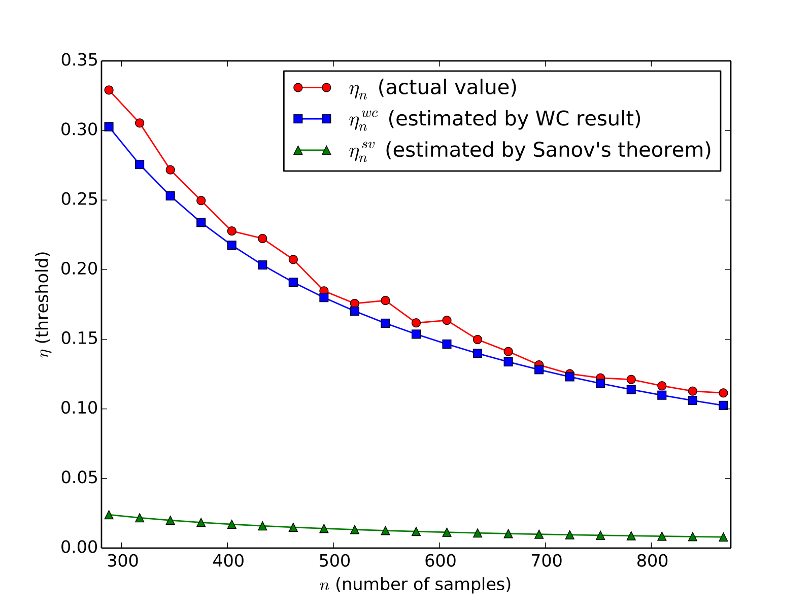
Let the false alarm probability be $\beta_{n}=\beta=0.001$. We set the aforementioned parameters as $N=12$, $\varepsilon=10^{-8}$, $T=1000$, $m_{0}=1000$, and let $n_{0}=1000N^{2}$. In Fig. 1, the red line indicates the theoretical value of the threshold $\eta_{n}$, the blue line shows the WC approximation $\eta_{n}^{wc}$, and the green line demonstrates the estimate $\eta_{n}^{sv}$ obtained by Sanov’s theorem, all as a function of the number of samples $n$. It is seen that $\eta_{n}^{wc}$ is much more accurate than $\eta_{n}^{sv}$.

Figure 1: Threshold ($\eta$) versus number of samples ($n$); the number of states in the original Markov chain is $N=12$.

Remark 3: In Fig. 1, the red line corresponding to the actual value $\eta_{n}$ is not as smooth; the reason is that each time when varying the number of samples $n$, we regenerate all the samples ${\mathbf{Z}}^{\scriptscriptstyle{\left(t\right)}}=\big{\{}{Z_{1}^{\scriptscriptstyle{\left(t\right)}},\ldots,Z_{n}^{\scriptscriptstyle{\left(t\right)}}}\big{\}},~{}t=1,\ldots,T$, from scratch. On the other hand, the blue line corresponding to $\eta_{n}^{wc}$ looks smooth; this is because we only need to generate the $T$ Gaussian sample vectors according to $\mathcal{N}({0,~{}\hat{\bm{\Lambda}}})$ once. Note that, in our experiments, most of the running time is spent generating the samples ${{\mathbf{Z}}^{\scriptscriptstyle{\left(t\right)}}}=\big{\{}{Z_{1}^{\scriptscriptstyle{\left(t\right)}},\ldots,Z_{n}^{\scriptscriptstyle{\left(t\right)}}}\big{\}},~{}t=1,\ldots,T$, and then calculating $\eta_{n}$. In practice, when implementing the approximation procedure proposed in this subsection, we will only need to focus on obtaining $\eta_{n}^{wc}$, which is computationally inexpensive.

IV-B Simulation results for network anomaly detection

We will use the term traffic and flow interchangeably in this subsection; they mean the same thing. The simulations are done using the software package SADIT [11], which, based on the fs-simulator [19], can efficiently generate flow-level network traffic datasets with annotated anomalies.

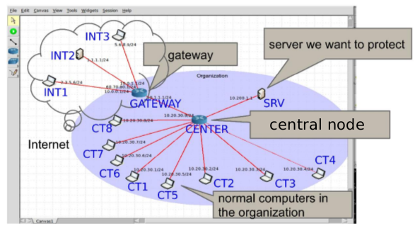
The network (see Fig. 2) consists of an internal network involving 8 normal users (CT1-CT8) and 1 server (SRV) that stores some sensitive information, and 3 Internet nodes (INT1-INT3) that visit the internal network via a gateway (GATEWAY).

Figure 2: Simulation setting (this figure is from [4] (or, see [20])).

When dealing with the data, we use the features “flow duration,” “flow size,” and “distance to cluster center” (this is related to a user IP address). The data preprocessing involves three steps: i) network traffic representation and flow aggregation, ii) quantization, and iii) window aggregation; cf. [4, Sec. iii@.A].

To implement Hoeffding’s test, we first estimate a PL (resp., a set of PLs) for the stationary (resp., time-varying) normal traffic. For the former case, we use as the reference traffic the whole flow sequence with anomalies at some time interval that we seek to detect. For the latter case, we generate the reference traffic and the traffic with anomalies separately, sharing all of the parameters except the ones regarding the anomalies. Using the windowing technique [20], [4], we then persistently monitor the traffic and report anomalies instantly whenever the relative entropy is higher than the threshold corresponding to the detection window.

The key difference between the whole detection procedures for the two types of traffic is that, estimating a PL for the stationary traffic is straightforward, while, for the time-varying traffic, we need to make an effort to identify several different PLs corresponding to certain time intervals. We apply the two-steps procedure proposed in [4]; that is, with some rough estimation of the shifting and periodic parameters of the traffic, we first generate a large set of PLs, and then refine the large family of PLs by solving a weighted set cover problem. For further theoretical details and the implementation, the reader is referred to [4], [11].

Note that, to deal with the time-varying traffic, [4] proposes a generalized Hoeffding’s test, which we will use for Scenario 2 in the following. However, there is no essential difference compared to the typical Hoeffding’s test. Note also that, in the following experiments, we only use the model-based method [20], [4].

IV-B1 Scenario 1 (Stationary Network Traffic)

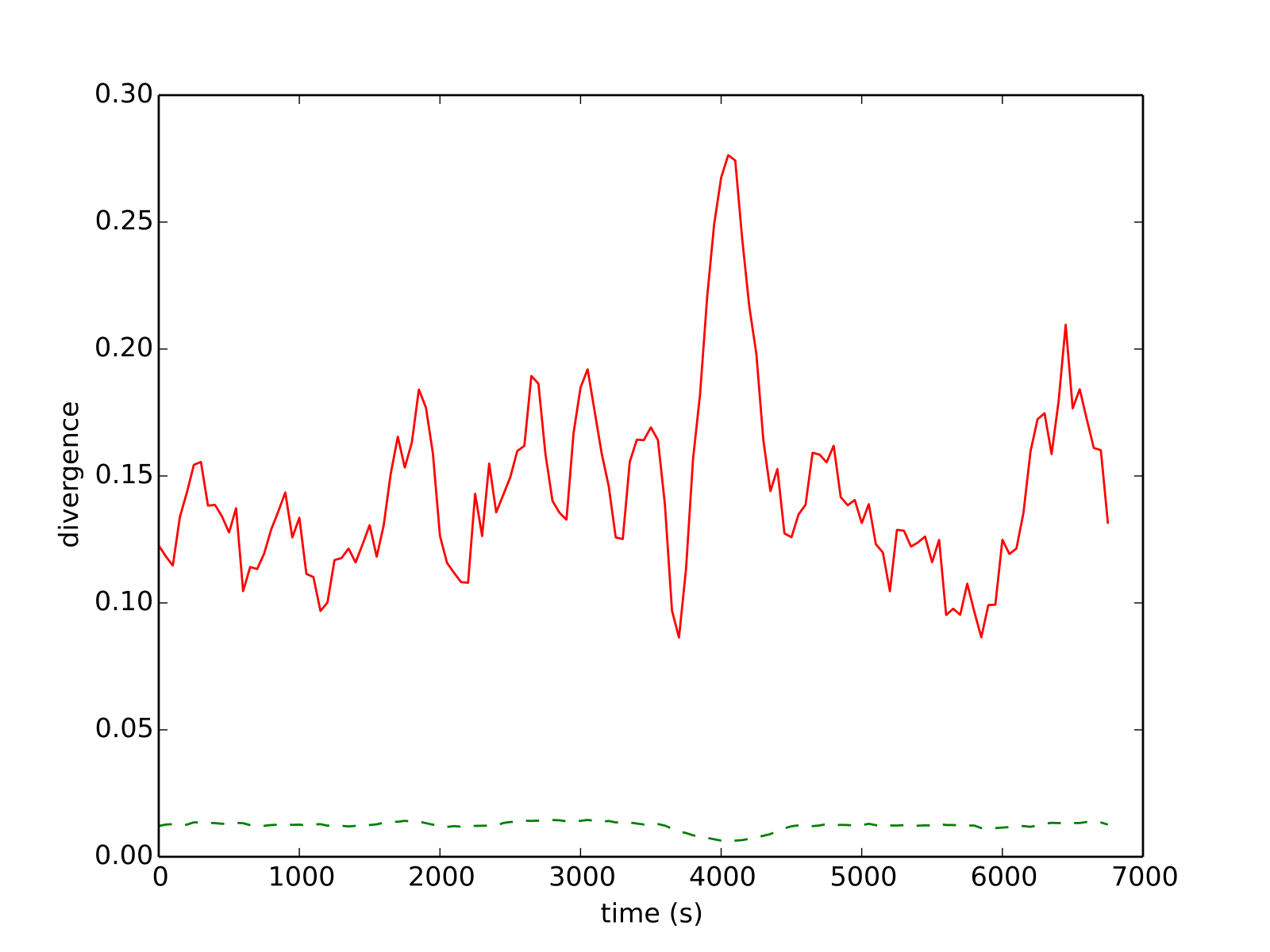
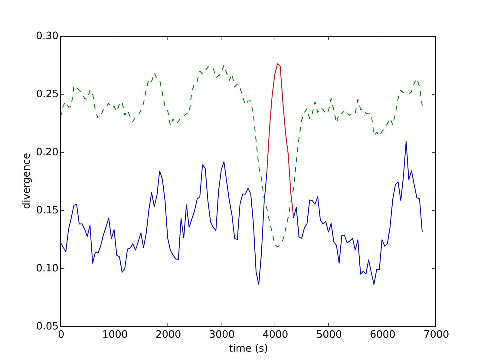
We mimic the case for anomaly caused by “large access rate;” cf. [20, Sec. iv@.A.3]. The simulation time is $7000$ s. A user suspiciously increases its access rate to 10 times of its normal value between $4000$ s and $4500$ s. The interval between the starting point of two consecutive time windows is taken as $50$ s, the window-size is chosen to be $w_{s}=400$ s, and the false alarm probability is set as $\beta=0.001$.

Set the quantization level for “flow duration,” “flow size,” and “distance to cluster center” to be $n_{1}=1$, $n_{2}=2$, and $n_{3}=2$, respectively. Set the number of user clusters as $k=3$.

Figure 3: Detection result for Scenario 1 with $w_{s}=400$ s, $n_{1}=1$, $n_{2}=2$, $n_{3}=2$, $k=3$; threshold is estimated by use of Sanov’s theorem.

Figure 4: Detection result for Scenario 1 with $w_{s}=400$ s, $n_{1}=1$, $n_{2}=2$, $n_{3}=2$, $k=3$; threshold is estimated by use of weak convergence result.

See Fig. 3 and Fig. 4 for the detection results. Both figures depict the relative entropy (divergence) metric in (2). The green dashed line in Fig. 3 is the threshold calculated using Sanov’s theorem (i.e., $\eta_{n}^{sv}$, where $n$ is the number of flows in a specific detection window). The green dashed line in Fig. 4 is the threshold computed using the WC result derived in Sec. iii@ (i.e., $\eta_{n}^{wc}$). The interval during which the entropy curve is above the threshold line (the red part) is the interval reported as abnormal.

Fig. 3 shows that, if using $\eta_{n}^{sv}$ as the threshold, then the detection method reports an anomaly for all windows including the ones wherein the behavior of the network traffic is actually normal; in other words, there are too many false alarms. Clearly, this is undesirable. Fig. 4 shows that, if, instead, we use $\eta_{n}^{wc}$ as the threshold, then the detection method will not report any false alarm while successfully identifying the true anomalies between $4000$ s and $4500$ s. The reason for such detection results is that $\eta_{n}^{wc}$ is more accurate than $\eta_{n}^{sv}$.

IV-B2 Scenario 2 (Time-Varying Network Traffic)

Consider the network with day-night pattern where the flow size follows a log-normal distribution. We use exactly the same scenario as that in [4, Sec. iv@.B.2].

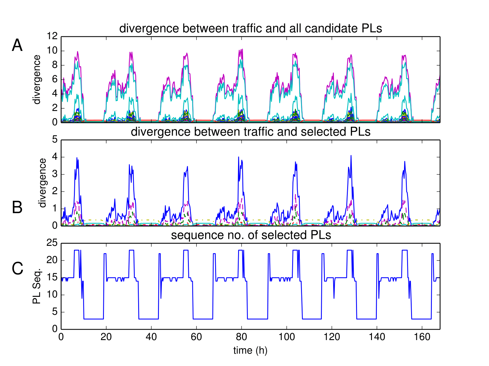
Applying the same procedure as in [4, Sec. iii@.C], we first obtain $32$ rough PLs. Then, using the heuristic PL refinement algorithm given in [4, Sec. iii@.D] equipped with the up-bound nominal cross-entropy parameter $\lambda=0.027565$, which is determined by the WC approximation, we finally obtain $6$ PLs (see Fig. 5). These PLs are active during morning, afternoon, evening, mid-night, dawn, and the transition time around sunrise, respectively. In the following detection procedure, the key difference between our method and the one used in [4] is that we no longer manually set the threshold universally as a constant; instead, the threshold $\eta_{n}^{wc}$ for each detection window is automatically calculated by use of the WC approximation. We set the quantization level for “flow duration,” “flow size,” and “distance to cluster center” to be $n_{1}=1$, $n_{2}=4$, and $n_{3}=1$, respectively, and set the number of user clusters to $k=1$. The interval between the starting point of two consecutive time windows is chosen as $1000$ s, the window-size is taken as $w_{s}=1000$ s, and the false alarm probability is set as $\beta=0.001$.

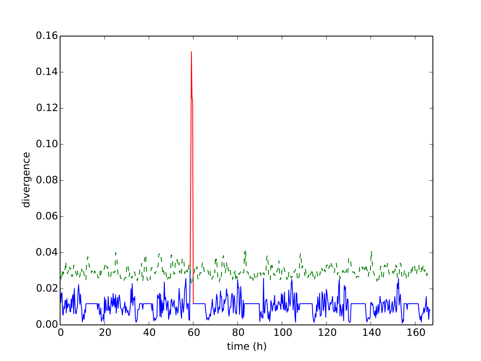
Noting that the anomaly is simulated beginning at 59 h and lasting for 80 minutes [4], we see from Fig. 6 that the anomaly is successfully detected, without any false alarms.

Figure 5: PLs identification for Scenario 2 with $w_{s}=1000$ s, $n_{1}=1$, $n_{2}=4$, $n_{3}=1$, $k=1$.

Figure 6: Detection result for Scenario 2 with $w_{s}=1000$ s, $n_{1}=1$, $n_{2}=4$, $n_{3}=1$, $k=1$.

V Conclusions

We establish a weak convergence result for the relative entropy in Hoeffding’s test under a Markovian assumption, which enables us to obtain a more accurate approximation (compared to the existing approximation given by Sanov’s theorem) for the threshold needed by the test. We validate the accuracy of such approximation through numerical experiments and simulations for network anomaly detection.

References

• [1] A. Dembo and O. Zeitouni, Large deviations techniques and applications.   Springer, 1998.
• [2] I. C. Paschalidis and G. Smaragdakis, “Spatio-temporal network anomaly detection by assessing deviations of empirical measures,” IEEE/ACM Transactions on Networking (TON), vol. 17, no. 3, pp. 685–697, 2009.
• [3] S. Meyn, A. Surana, Y. Lin, and S. Narayanan, “Anomaly detection using projective Markov models in a distributed sensor network,” in Proceedings of the 48th IEEE Conference on Decision and Control, 2009 held jointly with the 2009 28th Chinese Control Conference. CDC/CCC 2009., Dec 2009, pp. 4662–4669.
• [4] J. Wang and I. Paschalidis, “Statistical traffic anomaly detection in time-varying communication networks,” IEEE Transactions on Control of Network Systems, vol. 2, no. 2, pp. 100–111, 2015.
• [5] J. Unnikrishnan and D. Huang, “Weak convergence analysis of asymptotically optimal hypothesis tests,” IEEE Transactions on Information Theory, submitted, 2013.
• [6] W. Hoeffding, “Asymptotically optimal tests for multinomial distributions,” The Annals of Mathematical Statistics, pp. 369–401, 1965.
• [7] J. Zhang, “Threshold Approximation for Hoeffding’s Test under I.I.D. Assumption (TAHTIID),” https://github.com/jingzbu/TAHTIID, 2015.
• [8] J. Unnikrishnan, D. Huang, S. P. Meyn, A. Surana, and V. V. Veeravalli, “Universal and composite hypothesis testing via mismatched divergence,” IEEE Transactions on Information Theory, vol. 57, no. 3, pp. 1587–1603, 2011.
• [9] S. S. Wilks, “The large-sample distribution of the likelihood ratio for testing composite hypotheses,” The Annals of Mathematical Statistics, vol. 9, no. 1, pp. 60–62, 1938.
• [10] M. Iltis, “Sharp asymptotics of large deviations in dsuperscript𝑑\mathbb{R}^{d},” Journal of Theoretical Probability, vol. 8, no. 3, pp. 501–522, 1995.
• [11] J. Wang, J. Zhang, and I. C. Paschalidis, “Systematic Anomaly Detection of Internet Traffic (SADIT),” https://github.com/hbhzwj/SADIT, 2014.
• [12] G. L. Jones, “On the Markov chain central limit theorem,” Probability Surveys, vol. 1, pp. 299–320, 2004.
• [13] S. P. Meyn and R. L. Tweedie, Markov Chains and Stochastic Stability.   New York: Springer, 1993.
• [14] G. O. Roberts and J. S. Rosenthal, “General state space Markov chains and MCMC algorithms,” Probability Surveys, vol. 1, pp. 20–71, 2004.
• [15] F. Pène, “Rate of convergence in the multidimensional central limit theorem for stationary processes. Application to the Knudsen gas and to the Sinai billiard,” The Annals of Applied Probability, vol. 15, no. 4, pp. 2331–2392, 2005.
• [16] W. Feller, An introduction to probability theory and its applications.   John Wiley, 1957, vol. 2.
• [17] J. Zhang, “Threshold Approximation for Hoeffding’s Test under Markovian Assumption (TAHTMA),” https://github.com/jingzbu/TAHTMA, 2015.
• [18] R. A. Horn and C. R. Johnson, Matrix analysis.   Cambridge university press, 2012.
• [19] J. Sommers, R. Bowden, B. Eriksson, P. Barford, M. Roughan, and N. Duffield, “Efficient network-wide flow record generation,” in INFOCOM, 2011 Proceedings IEEE.   IEEE, 2011, pp. 2363–2371.
• [20] J. Wang, D. Rossell, C. G. Cassandras, and I. C. Paschalidis, “Network anomaly detection: A survey and comparative analysis of stochastic and deterministic methods,” in IEEE 52nd Annual Conference on Decision and Control (CDC), Dec 2013, pp. 182–187.