Newton-like method with diagonal correction for distributed optimization

Dragana Bajović 111Department of Power, Electronics and Communication Engineering, Faculty of Technical Sciences, University of Novi Sad, Trg Dositeja Obradovića 6, 21000 Novi Sad, Serbia. email: dbajovic@uns.ac.rs. 222Biosense Institute, University of Novi Sad, Ul. Zorana Djindjića 3, 21000 Novi Sad, Serbia.    Dušan Jakovetić 33footnotemark: 3    Nataša Krejić 333Department of Mathematics and Informatics, Faculty of Sciences, University of Novi Sad, Trg Dositeja Obradovića 4, 21000 Novi Sad, Serbia. e-mail: {djakovet@uns.ac.rs, natasak@uns.ac.rs, natasa.krklec@dmi.uns.ac.rs}. Research supported by the Serbian Ministry of Education, Science, and Technological Development, Grant no. 174030    Nataša Krklec Jerinkić 33footnotemark: 3
Abstract

We consider distributed optimization problems where networked nodes cooperatively minimize the sum of their locally known convex costs. A popular class of methods to solve these problems are the distributed gradient methods, which are attractive due to their inexpensive iterations, but have a drawback of slow convergence rates. This motivates the incorporation of second order information in the distributed methods, but this task is challenging: although the Hessians which arise in the algorithm design respect the sparsity of the network, their inverses are dense, hence rendering distributed implementations difficult. We overcome this challenge and propose a class of distributed Newton-like methods, which we refer to as Distributed Quasi Newton (DQN). The DQN family approximates the Hessian inverse by: 1) splitting the Hessian into its diagonal and off-diagonal part, 2) inverting the diagonal part, and 3) approximating the inverse of the off-diagonal part through a weighted linear function. The approximation is parameterized by the tuning variables which correspond to different splittings of the Hessian and by different weightings of the off-diagonal Hessian part. Specific choices of the tuning variables give rise to different variants of the proposed general DQN method – dubbed DQN-0, DQN-1 and DQN-2 – which mutually trade-off communication and computational costs for convergence. Simulations demonstrate the effectiveness of the proposed DQN methods.

Key words: Distributed optimization, second order methods, Newton-like methods, linear convergence.

AMS subject classification. 90C25, 90C53, 65K05

1 Introduction

We consider a connected network with n𝑛n nodes, each of which has access to a local cost function fi:p,i=1,,n.:subscript𝑓𝑖formulae-sequencesuperscript𝑝𝑖1𝑛f_{i}:\mathbb{R}^{p}\rightarrow\mathbb{R},\;i=1,\ldots,n. The objective for all nodes is to minimize the aggregate cost function f:p:𝑓superscript𝑝f:\mathbb{R}^{p}\rightarrow\mathbb{R}, defined by

f(y)=i=1nfi(y).𝑓𝑦superscriptsubscript𝑖1𝑛subscript𝑓𝑖𝑦f(y)=\sum_{i=1}^{n}f_{i}(y). (1)

Problems of this form arise in many emerging applications like big data analytics, e.g., [7], distributed inference in sensor networks [33, 16, 21, 5], and distributed control, [29].

Various methods for solving (1) in a distributed manner are available in the literature. A class of methods based on gradient descent at each node and exchange of information between neighboring nodes is particularly popular, see [30, 31, 32, 14, 15, 6, 40, 36, 20]. Assuming that the local costs fisubscript𝑓𝑖f_{i}’s are strongly convex and have Lipschitz continuous gradients and that a constant step size α𝛼\alpha is used, these methods converge linearly to a solution neighborhood. With such methods, step size α𝛼\alpha controls the tradeoff between the convergence speed towards a solution neighborhood and the distance of the limit point from the actual solution, larger α𝛼\alpha means faster convergence but larger distance from the solution in the limit; see, e.g., [15], [22]. Distributed first order (gradient) methods allow for a penalty interpretation, where the distributed method is interpreted as a (centralized) gradient method applied on a carefully constructed penalty reformulation of the original problem (1); see [15], [22] for details.

Given the existence of well developed theory and efficient implementations of higher order methods in centralized optimization in general, there is a clear need to investigate the possibilities of employing higher order methods in distributed optimization as well. More specifically, for additive cost structures (1) we study here, a further motivation for developing distributed higher order methods comes from their previous success when applied to similar problems in the context of centralized optimization. For example, additive cost (1) is typical in machine learning applications where second order methods play an important role, see, e.g., [2, 3, 4]. Another similar class of problems arise in stochastic optimization, where the objective function is given in the form of mathematical expectation. Again, second order methods are successfully applied in centralized optimization, [12, 17, 18, 25, 26].

There have been several papers on distributed Newton-type methods. A distributed second order methods for network utility maximization and network flow optimization are developed in [37] and [41] but on problem formulations different from (1). Network Newton method [22] aims at solving (1) and presents a family of distributed (approximate) Newton methods. The class of Netwrok Newton method, refereed to as NN, is extensively analyzed in [23, 24]. The proposed methods are based on the penalty interpretation, [15, 22], of the distributed gradient method in [30], and they approximate the Newton step through an \ell-th order Taylor approximation of the Hessian inverse, =0,1,01\ell=0,1,... This approximation gives rise to different variants of methods within the family, dubbed NN-\ell. Different choices of \ell exhibit inherent tradeoffs between the communication cost and the number of iterations until convergence, while NN-00, 111, and 222 are the most efficient in practice. The proposed methods converge linearly to a solution neighborhood, exhibit a kind of quadratic convergence phase, and show significantly better simulated performance when compared with the standard distributed gradient method in [30]. Reference [27] proposes a distributed second order method which approximates the (possibly expensive) primal updates with the distributed alternating direction of multipliers method in [35]. In [38], the authors propose a distributed Newton Raphson method based on the consensus algorithm and separation of time-scales. Reference [28] proposes distributed second order methods based on the proximal method of multipliers (PMM). Specifically, the methods approximate the primal variable update step through a second order approximation of the NN-type [22]. While the NN methods in [22] converge to a solution neighborhood, the methods in [28, 27, 38] converge to exact solutions.

In this paper, we extend [22, 23, 24] and propose a different family of distributed Newton-like methods for solving (1). We refer to the proposed family as Distributed Quasi Newton methods (DQN). The methods are designed to exploit the specific structure of the penalty reformulation [15, 22], as is done in [22], but with a different Hessian inverse approximation, for which the idea originates in [19]. Specifically, the Hessian matrix is approximated by its block diagonal part, while the remaining part of the Hessian is used to correct the right hand side of the quasi Newton equation. The methods exhibit linear convergence to a solution neighborhood under a set of standard assumptions for the functions fisubscript𝑓𝑖f_{i} and the network architecture – each fisubscript𝑓𝑖f_{i} is strongly convex and has Lipschitz continuous gradient, and the underlying network is connected. Simulation examples on (strongly convex) quadratic and logistic losses demonstrate that DQN compares favorably with NN proposed in [22].

With the DQN family of methods, the approximation of the Newton step is parameterized by diagonal matrix 𝕃ksubscript𝕃𝑘\mathbb{L}_{k} at each iteration k𝑘k, and different choices of 𝕃ksubscript𝕃𝑘\mathbb{L}_{k} give rise to different variants of DQN, which we refer to as DQN-00, 111, and 222. Different variants of DQN, based on different matrices 𝕃ksubscript𝕃𝑘\mathbb{L}_{k}, tradeoff the number of iterations and computational cost. In particular, setting 𝕃k=0subscript𝕃𝑘0\mathbb{L}_{k}=0 yields the DQN-0 method; a constant, diagonal matrix 𝕃k=𝕃subscript𝕃𝑘𝕃\mathbb{L}_{k}=\mathbb{L} corresponds to DQN-1. Finally, 𝕃ksubscript𝕃𝑘\mathbb{L}_{k} with DQN-2 is obtained through approximately fitting the Newton equation (34) using a first order Taylor approximation. The DQN-1 method utilizes the latter, DQN-2’s weight matrix at the first iteration, and then it “freezes” it to this constant value throughout the iterations; that is, it sets 𝕃=𝕃0𝕃subscript𝕃0\mathbb{L}=\mathbb{L}_{0}, where 𝕃0subscript𝕃0\mathbb{L}_{0} corresponds to the weight matrix of DQN-2 in the initial iteration.

Let us further specify the main differences between the proposed DQN family and NN methods in [22] as the NN methods are used as the benchmark in the work presented here. First, the DQN methods introduce a different, more general splitting of Hessians with respect to NN, parameterized with a scalar θ0𝜃0\theta\geq 0; in contrast, the splitting used in NN corresponds to setting θ=1𝜃1\theta=1. Second, with the proposed variants of DQN-00, 111, and 222, we utilize diagonal matrices 𝕃ksubscript𝕃𝑘\mathbb{L}_{k}, while the NN-\ell methods use in general block-diagonal or neighbor-sparse matrices. Third, DQN and NN utilize different inverse Hessian approximations; the NN’s inverse Hessian approximation matrix is symmetric, while with DQN it is not symmetric in general. Fourth, while NN approximates the inverse Hessian directly (independently of the Newton equation), DQN actually aims at approximating the Newton equation. Hence, unlike NN, the resulting DQN’s inverse Hessian approximation (with DQN-2 in particular) explicitly depends on the gradient at the current iterate, as it is the case with many Quasi-Newton methods; see, e.g., [9]. Finally, the analysis here is very different from [22], and the major reason comes from the fact that the Hessian approximation with DQN is asymmetric in general. This fact also incurs the need for a safeguarding step with DQN in general, as detailed in Section 3. We also point out that results presented in [22] show that NN methods exhibit a quadratic convergence phase. It is likely that similar results can be shown for certain variants of DQN methods as well, but detailed analysis is left for future work. It may be very challenging to rigorously compare the linear convergence rate factors of DQN and NN methods and their respective inverse Hessian approximations. However, we provide in Section 5 both certain analytical insights and extensive numerical experiments to compare the two classes of methods.

As noted, DQN methods do not converge to the exact solution of (1), but they converge to a solution neighborhood, as it is the case with other methods (e.g., distributed gradient descent [30] and NN methods [22]) which are based on the penalty interpretation of (1). Hence, for very high accuracies, they may not be competitive with distributed second order methods which converge to the exact solution [27, 28, 38]. However, following the framework of embedding distributed second order methods into PMM – developed in [28], we apply here the DQN Newton direction approximations to the PMM methods; we refer to the resulting methods as PMM-DQN-\ell, =0,1,2012\ell=0,1,2. Simulation examples on strongly convex quadratic costs demonstrate that the PMM-DQN methods compare favorably with the methods in [27, 28, 38]. Therefore, with respect to the existing literature and in particular with respect to [22, 28], this paper broadens the possibilities for distributed approximations of relevant Newton directions, and hence offers alternative distributed second order methods, which exhibit competitive performance on the considered simulation examples. Analytical studies of PMM-DQN are left for future work.

This paper is organized as follows. In Section 2 we give the problem statement and some preliminaries needed for the definition of the method and convergence analysis. Section 3 contains the description of the proposed class of Newton-like methods and convergence results. Specific choices of the diagonal matrix that specifies the method completely are presented in Section 4. Some simulation results are presented in Section 5 while Section 6 discusses extensions of embedding DQN in the PMM framework. Finally, conclusions are drawn in Section 7, while Appendix provides some auxiliary derivations.

2 Preliminaries

Let us first give some preliminaries about the problem (1), its penalty interpretation in [15, 22], as well as the decentralized gradient descent algorithm in [30] that will be used later on.

The following assumption on the fisubscript𝑓𝑖f_{i}’s is imposed.

Assumption A1. The functions fi:p,i=1,,n:subscript𝑓𝑖formulae-sequencesuperscript𝑝𝑖1𝑛f_{i}:\mathbb{R}^{p}\rightarrow\mathbb{R},\;i=1,\ldots,n are twice continuously differentiable, and there exist constants 0<μL<0𝜇𝐿0<\mu\leq L<\infty such that for every xp𝑥superscript𝑝x\in\mathbb{R}^{p}

μI2fi(x)LI.precedes-or-equals𝜇𝐼superscript2subscript𝑓𝑖𝑥precedes-or-equals𝐿𝐼\mu I\preceq\nabla^{2}f_{i}(x)\preceq LI.

Here, I𝐼I denotes the p×p𝑝𝑝p\times p identity matrix, and notation MNprecedes-or-equals𝑀𝑁M\preceq N means that the matrix NM𝑁𝑀N-M is positive semi-definite.

This assumption implies that the functions fi,i=1,,nformulae-sequencesubscript𝑓𝑖𝑖1𝑛f_{i},\;i=1,\ldots,n are strongly convex with modulus μ>0,𝜇0\mu>0,

fi(z)fi(y)+fi(y)T(zy)+μ2zy2,y,zp,formulae-sequencesubscript𝑓𝑖𝑧subscript𝑓𝑖𝑦subscript𝑓𝑖superscript𝑦𝑇𝑧𝑦𝜇2superscriptnorm𝑧𝑦2𝑦𝑧superscript𝑝f_{i}(z)\geq f_{i}(y)+\nabla f_{i}(y)^{T}(z-y)+\frac{\mu}{2}\|z-y\|^{2},\;y,z\in\mathbb{R}^{p}, (2)

and the gradients are Lipschitz continuous with the constant L𝐿L i.e.

fi(y)fi(z)Lyz,y,zp,i=1,,n.formulae-sequencenormsubscript𝑓𝑖𝑦subscript𝑓𝑖𝑧𝐿norm𝑦𝑧𝑦formulae-sequence𝑧superscript𝑝𝑖1𝑛\|\nabla f_{i}(y)-\nabla f_{i}(z)\|\leq L\|y-z\|,\;y,z\in\mathbb{R}^{p},\;i=1,\ldots,n. (3)

Assume that the network of nodes is an undirected network 𝒢=(𝒱,),𝒢𝒱{\mathcal{G}}=({\mathcal{V}},{\mathcal{E}}), where 𝒱𝒱{\mathcal{V}} is the set of nodes and {\mathcal{E}} is the set of all edges, i.e., all pairs {i,j}𝑖𝑗\{i,j\} of nodes which can exchange information through a communication link.

Assumption A2. The network 𝒢=(𝒱,)𝒢𝒱{\mathcal{G}}=({\mathcal{V}},{\mathcal{E}}) is connected, undirected and simple (no self-loops nor multiple links).

Let us denote by Oisubscript𝑂𝑖O_{i} the set of nodes that are connected with the node i𝑖i (open neighborhood of node i𝑖i) and let O¯i=Oi{i}subscript¯𝑂𝑖subscript𝑂𝑖𝑖\bar{O}_{i}=O_{i}\bigcup\{i\} (closed neighborhood of node i𝑖i). We associate with 𝒢𝒢{\mathcal{G}} a symmetric, (doubly) stochastic n×n𝑛𝑛n\times n matrix W.𝑊W. The elements of W𝑊W are all nonnegative and rows (and columns) sum up to one. More precisely, we assume the following.

Assumption A3. The matrix W=WTn×n𝑊superscript𝑊𝑇superscript𝑛𝑛W=W^{T}\in\mathbb{R}^{n\times n} is stochastic with elements wijsubscript𝑤𝑖𝑗w_{ij} such that

wij>0 if {i,j},wij=0 if {i,j},ij, and wii=1jOiwijformulae-sequencesubscript𝑤𝑖𝑗0 if 𝑖𝑗subscript𝑤𝑖𝑗0 if 𝑖𝑗formulae-sequence𝑖𝑗 and subscript𝑤𝑖𝑖1subscript𝑗subscript𝑂𝑖subscript𝑤𝑖𝑗w_{ij}>0\mbox{ if }\{i,j\}\in{\mathcal{E}},\;w_{ij}=0\mbox{ if }\{i,j\}\notin{\mathcal{E}},\,i\neq j,\mbox{ and }w_{ii}=1-\sum_{j\in O_{i}}w_{ij}

and there are constants wminsubscript𝑤𝑚𝑖𝑛w_{min} and wmaxsubscript𝑤𝑚𝑎𝑥w_{max} such that for i=1,,n𝑖1𝑛i=1,\ldots,n

0<wminwiiwmax<1.0subscript𝑤𝑚𝑖𝑛subscript𝑤𝑖𝑖subscript𝑤𝑚𝑎𝑥10<w_{min}\leq w_{ii}\leq w_{max}<1.

Denote by λ1λnsubscript𝜆1subscript𝜆𝑛\lambda_{1}\geq\ldots\geq\lambda_{n} the eigenvalues of W.𝑊W. Then it can be easily seen that λ1=1.subscript𝜆11\lambda_{1}=1. Furthermore, the null space of IW𝐼𝑊I-W is spanned by e:=(1,,1).assign𝑒11e:=(1,\ldots,1).

Following [15], [22], the auxiliary function Φ:np,:Φsuperscript𝑛𝑝\Phi:\mathbb{R}^{np}\rightarrow\mathbb{R}, and the corresponding penalty reformulation of (1) is introduced as follows. Let x=(x1,,xn)np𝑥subscript𝑥1subscript𝑥𝑛superscript𝑛𝑝x=(x_{1},\ldots,x_{n})\in\mathbb{R}^{np} with xip,subscript𝑥𝑖superscript𝑝x_{i}\in{\mathbb{R}}^{p}, and denote by np×npsuperscript𝑛𝑝𝑛𝑝\mathbb{Z}\in\mathbb{R}^{np\times np} the matrix obtained as the Kronecker product of W𝑊W and the identity I𝐑p×p,=WI.formulae-sequence𝐼superscript𝐑𝑝𝑝tensor-product𝑊𝐼I\in\mathbf{R}^{p\times p},\mathbb{Z}=W\otimes I.

The corresponding penalty reformulation of (1) is given by

minxnpΦ(x):=αi=1nfi(xi)+12xT(𝕀)x.assignsubscript𝑥superscript𝑛𝑝Φ𝑥𝛼superscriptsubscript𝑖1𝑛subscript𝑓𝑖subscript𝑥𝑖12superscript𝑥𝑇𝕀𝑥\min_{x\in{\mathbb{R}^{np}}}\Phi(x):=\alpha\sum_{i=1}^{n}f_{i}(x_{i})+\frac{1}{2}x^{T}({\mathbb{I}}-\mathbb{Z})x. (4)

Applying the standard gradient method to (4) with the unit step size we get

xk+1=xkΦ(xk),k=0,1,,formulae-sequencesuperscript𝑥𝑘1superscript𝑥𝑘Φsuperscript𝑥𝑘𝑘01x^{k+1}=x^{k}-\nabla\,\Phi(x^{k}),\,k=0,1,..., (5)

which, denoting the i𝑖i-th p×1𝑝1p\times 1 block of xksuperscript𝑥𝑘x^{k} by xik,superscriptsubscript𝑥𝑖𝑘x_{i}^{k}, and after rearranging terms, yields the Decentralized Gradient Descent (DGD) method [30]

xik+1=jO¯iwijxjkαfi(xik),i=1,,n.formulae-sequencesuperscriptsubscript𝑥𝑖𝑘1subscript𝑗subscript¯𝑂𝑖subscript𝑤𝑖𝑗superscriptsubscript𝑥𝑗𝑘𝛼subscript𝑓𝑖superscriptsubscript𝑥𝑖𝑘𝑖1𝑛x_{i}^{k+1}=\sum_{j\in\bar{O}_{i}}w_{ij}\,x_{j}^{k}-\alpha\nabla f_{i}(x_{i}^{k}),\;i=1,\ldots,n. (6)

Clearly, the penalty parameter α𝛼\alpha influences the relation between (4) and (1) – a smaller α𝛼\alpha means better agreement between the problems but also implies smaller steps in (6) and thus makes the convergence slower. It can be shown, [22] that if y~p~𝑦superscript𝑝\tilde{y}\in\mathbb{R}^{p} is the solution of (1) and x:=(y¯1,,y¯n)npassignsuperscript𝑥subscript¯𝑦1subscript¯𝑦𝑛superscript𝑛𝑝x^{*}:=(\bar{y}_{1},\ldots,\bar{y}_{n})\in\mathbb{R}^{np} is the solution of (4) then, for all i𝑖i,

y¯iy~=𝒪(α).normsubscript¯𝑦𝑖~𝑦𝒪𝛼\|\bar{y}_{i}-\tilde{y}\|={\mathcal{O}}(\alpha). (7)

The convergence of (6) towards xsuperscript𝑥x^{*} is linear, i.e., the following estimate holds [40, 15],

Φ(xk)Φ(x)(1ξ)k(Φ(x0)Φ(x)),Φsuperscript𝑥𝑘Φsuperscript𝑥superscript1𝜉𝑘Φsuperscript𝑥0Φsuperscript𝑥\Phi(x^{k})-\Phi(x^{*})\leq(1-\xi)^{k}(\Phi(x^{0})-\Phi(x^{*})), (8)

where ξ(0,1)𝜉01\xi\in(0,1) is a constant depending on Φ,αΦ𝛼\Phi,\alpha and W.𝑊W.

The matrix and vector norms that will be frequently used in the sequel are defined here. Let a2subscriptnorm𝑎2\|a\|_{2} denote the Euclidean norm of vector a𝑎a of arbitrary dimension. Next, A2subscriptnorm𝐴2\|A\|_{2} denotes the spectral norm of matrix A𝐴A of arbitrary dimension. Further, for a matrix 𝕄np×np𝕄superscript𝑛𝑝𝑛𝑝{\mathbb{M}}\in\mathbb{R}^{np\times np} with blocks Mijp×psubscript𝑀𝑖𝑗superscript𝑝𝑝M_{ij}\in\mathbb{R}^{p\times p}, we will also use the following block norm:

𝕄:=maxj=1,,ni=1nMij2,assignnorm𝕄subscript𝑗1𝑛superscriptsubscript𝑖1𝑛subscriptnormsubscript𝑀𝑖𝑗2\|{\mathbb{M}}\|:=\max_{j=1,\ldots,n}\sum_{i=1}^{n}\|M_{ij}\|_{2},

where, as noted, Mij2subscriptnormsubscript𝑀𝑖𝑗2\|M_{ij}\|_{2} is the spectral norm of Mijsubscript𝑀𝑖𝑗M_{ij}. For a vector xnp𝑥superscript𝑛𝑝x\in\mathbb{R}^{np} with blocks xipsubscript𝑥𝑖superscript𝑝x_{i}\in\mathbb{R}^{p}, the following block norm is also used:

x:=i=1nxi2.assignnorm𝑥superscriptsubscript𝑖1𝑛subscriptnormsubscript𝑥𝑖2\|x\|:=\sum_{i=1}^{n}\|x_{i}\|_{2}.

3 Distributed Quasi Newton method

In this section we introduce a class of Quasi Newton methods for solving (4). The general Distributed Quasi Newton (DQN) method is proposed in Subsection 3.1. The method is characterized by a generic diagonal matrix 𝕃k.subscript𝕃𝑘\mathbb{L}_{k}. Global linear convergence rate for the class is established in Subsection 3.2, while local linear convergence rate with the full step size ε=1𝜀1\varepsilon=1 is analyzed in Subsection 3.3. Specific variants DQN-00, 111, and 222, which correspond to the specific choices of 𝕃ksubscript𝕃𝑘\mathbb{L}_{k}, are studied in Section 4. As we will see, algorithm DQN has certain tuning parameters, including the step size ε𝜀\varepsilon. Discussion on the tuning parameters choice is relegated to Section 4.

3.1 The proposed general DQN method

The problem we consider from now on is (4), where we recall =WItensor-product𝑊𝐼\mathbb{Z}=W\otimes I and W𝑊W satisfies assumption A3.

The problem under consideration has a specific structure as the Hessian is sparse if the underlying network is sparse. However its inverse is dense. Furthermore, the matrix inversion (i.e. linear system solving) is not suitable for decentralized computation. One possibility of exploiting the structure of 2Φ(x)superscript2Φ𝑥\nabla^{2}\Phi(x) in a distributed environment is presented in [22] where the Newton step is approximated through a number of inner iterations. We present here a different possibility. Namely, we keep the diagonal part of 2Φ(x)superscript2Φ𝑥\nabla^{2}\Phi(x) as the Hessian approximation but at the same time use the non-diagonal part of 2Φ(x)superscript2Φ𝑥\nabla^{2}\Phi(x) to correct the right hand side vector in the (Quasi)-Newton equation. Let us define the splitting

Wd=diag(W)andWu=WWd,formulae-sequencesubscript𝑊𝑑𝑑𝑖𝑎𝑔𝑊andsubscript𝑊𝑢𝑊subscript𝑊𝑑W_{d}=diag(W)\quad\mbox{and}\quad W_{u}=W-W_{d},

and =d+usubscript𝑑subscript𝑢\mathbb{Z}=\mathbb{Z}_{d}+\mathbb{Z}_{u} with

d=WdI=diag()andu=WuI.formulae-sequencesubscript𝑑tensor-productsubscript𝑊𝑑𝐼𝑑𝑖𝑎𝑔andsubscript𝑢tensor-productsubscript𝑊𝑢𝐼\mathbb{Z}_{d}=W_{d}\otimes I=diag(\mathbb{Z})\quad\mbox{and}\quad\mathbb{Z}_{u}=W_{u}\otimes I.

Here, diag(W)𝑑𝑖𝑎𝑔𝑊diag(W) denotes the diagonal matrix with the same diagonal as the matrix W𝑊W. Hence, matrix dsubscript𝑑\mathbb{Z}_{d} is a np×np𝑛𝑝𝑛𝑝np\times np diagonal matrix whose i𝑖i-th p×p𝑝𝑝p\times p block is the scalar matrix wiiI,subscript𝑤𝑖𝑖𝐼w_{ii}I, usubscript𝑢\mathbb{Z}_{u} is a np×np𝑛𝑝𝑛𝑝np\times np block (symmetric) matrix such that (i,j)𝑖𝑗(i,j)-th p×p𝑝𝑝p\times p off-diagonal blocks are again scalar matrices wijIsubscript𝑤𝑖𝑗𝐼w_{ij}I, while the diagonal blocks are all equal to zero.

Clearly, the gradient is

Φ(x)=αF(x)+(𝕀)x,Φ𝑥𝛼𝐹𝑥𝕀𝑥\nabla\Phi(x)=\alpha\nabla F(x)+(\mathbb{I}-\mathbb{Z})x,

where 𝕀𝕀\mathbb{I} denotes the np×np𝑛𝑝𝑛𝑝np\times np identity matrix and

F(x)=i=1nfi(xi),F(x)=(f1(x1),,fn(xn)),formulae-sequence𝐹𝑥superscriptsubscript𝑖1𝑛subscript𝑓𝑖subscript𝑥𝑖𝐹𝑥subscript𝑓1subscript𝑥1subscript𝑓𝑛subscript𝑥𝑛F(x)=\sum_{i=1}^{n}f_{i}(x_{i}),\quad\nabla F(x)=(\nabla f_{1}(x_{1}),\ldots,\nabla f_{n}(x_{n})),

while the Hessian is

2Φ(x)=α2F(x)+𝕀superscript2Φ𝑥𝛼superscript2𝐹𝑥𝕀\nabla^{2}\Phi(x)=\alpha\nabla^{2}F(x)+\mathbb{I}-\mathbb{Z}

where 2F(x)superscript2𝐹𝑥\nabla^{2}F(x) is the block diagonal matrix with the i𝑖ith diagonal block 2fi(xi)superscript2subscript𝑓𝑖subscript𝑥𝑖\nabla^{2}f_{i}(x_{i}).

The general Distributed Quasi Newton, DQN, algorithm is presented below. Denote by k𝑘k the iteration counter, k=0,1,𝑘01k=0,1,..., and let xk=(x1k,,xnk)npsuperscript𝑥𝑘superscriptsubscript𝑥1𝑘superscriptsubscript𝑥𝑛𝑘superscript𝑛𝑝x^{k}=(x_{1}^{k},...,x_{n}^{k})\in{\mathbb{R}}^{np} be the estimate of xsuperscript𝑥x^{*} at iteration k𝑘k. Consider the following splitting of the Hessian

2Φ(xk)=𝔸k𝔾,superscript2Φsuperscript𝑥𝑘subscript𝔸𝑘𝔾\nabla^{2}\Phi(x^{k})={\mathbb{A}}_{k}-\mathbb{G}, (9)

with

𝔸k=α2F(xk)+(1+θ)(𝕀d)subscript𝔸𝑘𝛼superscript2𝐹superscript𝑥𝑘1𝜃𝕀subscript𝑑{\mathbb{A}}_{k}=\alpha\nabla^{2}F(x^{k})+(1+\theta)(\mathbb{I}-\mathbb{Z}_{d}) (10)

and

𝔾=u+θ(𝕀d)𝔾subscript𝑢𝜃𝕀subscript𝑑\mathbb{G}=\mathbb{Z}_{u}+\theta(\mathbb{I}-\mathbb{Z}_{d})

for some θ0𝜃0\theta\geq 0. Hence, 𝔾𝔾\mathbb{G} is a np×np𝑛𝑝𝑛𝑝np\times np block (symmetric) matrix whose i𝑖i-th p×p𝑝𝑝p\times p diagonal block equals giiIsubscript𝑔𝑖𝑖𝐼g_{ii}\,I, with gii:=θ(1wii)assignsubscript𝑔𝑖𝑖𝜃1subscript𝑤𝑖𝑖g_{ii}:=\theta\,(1-w_{ii}), while the (i,j)𝑖𝑗(i,j)-th p×p𝑝𝑝p\times p off-diagonal block equals gijIsubscript𝑔𝑖𝑗𝐼g_{ij}\,I, with gij:=wijassignsubscript𝑔𝑖𝑗subscript𝑤𝑖𝑗g_{ij}:=w_{ij}. One can easily see that the splitting above recovers the splitting for NN methods [22] taking θ=1.𝜃1\theta=1. We keep θ𝜃\theta unspecified for now and later on, we will demonstrate numerically that taking θ=0𝜃0\theta=0 can be beneficial. Also, notice that 𝔸ksubscript𝔸𝑘{\mathbb{A}}_{k} is block diagonal with the i𝑖ith diagonal block

Aik=α2fi(xik)+(1+θ)(1wii)I.subscriptsuperscript𝐴𝑘𝑖𝛼superscript2subscript𝑓𝑖subscriptsuperscript𝑥𝑘𝑖1𝜃1subscript𝑤𝑖𝑖𝐼A^{k}_{i}=\alpha\nabla^{2}f_{i}(x^{k}_{i})+(1+\theta)(1-w_{ii})I.

Let 𝕃knp×npsubscript𝕃𝑘superscript𝑛𝑝𝑛𝑝\mathbb{L}_{k}\in\mathbb{R}^{np\times np} be a diagonal matrix composed of diagonal p×p𝑝𝑝p\times p matrices Λik,i=1,,n.formulae-sequencesuperscriptsubscriptΛ𝑖𝑘𝑖1𝑛\Lambda_{i}^{k},\;i=1,\ldots,n. In this paper, we adopt the following approximation of the Newton direction sNk=(𝔸k𝔾)1Φ(xk)subscriptsuperscript𝑠𝑘𝑁superscriptsubscript𝔸𝑘𝔾1Φsuperscript𝑥𝑘s^{k}_{N}=-({\mathbb{A}}_{k}-\mathbb{G})^{-1}\nabla\Phi(x^{k}):

sk=(𝕀𝕃k𝔾)𝔸k1Φ(xk).superscript𝑠𝑘𝕀subscript𝕃𝑘𝔾subscriptsuperscript𝔸1𝑘Φsuperscript𝑥𝑘s^{k}=-(\mathbb{I}-\mathbb{L}_{k}\mathbb{G}){\mathbb{A}}^{-1}_{k}\nabla\Phi(x^{k}). (11)

The motivation for this approximation comes from [19] and the following reasoning. Keep the Hessian approximation on the left hand side of the Newton equation (𝔸k𝔾)sNk=Φ(xk)subscript𝔸𝑘𝔾subscriptsuperscript𝑠𝑘𝑁Φsuperscript𝑥𝑘({\mathbb{A}}_{k}-\mathbb{G})s^{k}_{N}=-\nabla\Phi(x^{k}) diagonal, and correct the right hand side through the off-diagonal Hessian part. In more detail, the Newton equation can be equivalently written as:

𝔸ksNk=Φ(xk)+𝔾sNk,subscript𝔸𝑘superscriptsubscript𝑠𝑁𝑘Φsuperscript𝑥𝑘𝔾subscriptsuperscript𝑠𝑘𝑁\mathbb{A}_{k}\,s_{N}^{k}=-\nabla\Phi(x^{k})+\mathbb{G}\,s^{k}_{N}, (12)

where the off-diagonal part s~k:=𝔾sNkassignsuperscript~𝑠𝑘𝔾subscriptsuperscript𝑠𝑘𝑁\mathaccent 869{s}^{k}:=\mathbb{G}\,s^{k}_{N} is moved to the right hand side. If we pretended for a moment to know the value of s~ksuperscript~𝑠𝑘\mathaccent 869{s}^{k}, then the Newton direction is obtained as:

sNk=(𝔸k)1(Φ(xk)s~k).subscriptsuperscript𝑠𝑘𝑁superscriptsubscript𝔸𝑘1Φsuperscript𝑥𝑘superscript~𝑠𝑘s^{k}_{N}=-\left(\mathbb{A}_{k}\right)^{-1}\left(\nabla\Phi(x^{k})-\mathaccent 869{s}^{k}\right). (13)

This form is suitable for distributed implementation due to the need to invert only the block diagonal matrix 𝔸ksubscript𝔸𝑘\mathbb{A}_{k}. However, s~ksuperscript~𝑠𝑘\mathaccent 869{s}^{k} is clearly not known, and hence we approximate it. To this end, note that, assuming that 𝔾Φ(xk)𝔾Φsuperscript𝑥𝑘\mathbb{G}\nabla\Phi(x^{k}) is a vector with all the entries being non-zero, without loss of generality, s~ksuperscript~𝑠𝑘\mathaccent 869{s}^{k} can be written as follows:

s~k=𝕃k𝔾Φ(xk),superscript~𝑠𝑘subscript𝕃𝑘𝔾Φsuperscript𝑥𝑘\mathaccent 869{s}^{k}=\mathbb{L}_{k}\,\mathbb{G}\,\nabla\Phi(x^{k}), (14)

where 𝕃ksubscript𝕃𝑘\mathbb{L}_{k} is a diagonal matrix. Therefore, estimating s~ksuperscript~𝑠𝑘\mathaccent 869{s}^{k} translates into estimating the diagonal matrix 𝕃ksubscript𝕃𝑘\mathbb{L}_{k}, assuming that 𝔾Φ(xk)𝔾Φsuperscript𝑥𝑘\mathbb{G}\,\nabla\Phi(x^{k}) is known. We follow [19] and consider simple approximations of the “true” 𝕃ksubscript𝕃𝑘\mathbb{L}_{k}. E.g., we will consider 𝕃k=0subscript𝕃𝑘0\mathbb{L}_{k}=0 which discards the off-diagonal Hessian part. Also, as we will see ahead, we adopt a Taylor approximation method for estimating 𝕃ksubscript𝕃𝑘\mathbb{L}_{k}. Now, substituting (14) into (13), we obtain the following Newton direction approximation:

s0k=(𝔸k)1(𝕀𝕃k𝔾)Φ(xk).superscriptsubscript𝑠0𝑘superscriptsubscript𝔸𝑘1𝕀subscript𝕃𝑘𝔾Φsuperscript𝑥𝑘s_{0}^{k}=-\left(\mathbb{A}_{k}\right)^{-1}\left(\mathbb{I}-\mathbb{L}_{k}\,\mathbb{G}\right)\nabla\Phi(x^{k}). (15)

Finally, we adopt (11) as the definite form of the Newton direction approximation, i.e., we permute the matrices (𝕀𝕃k𝔾)𝕀subscript𝕃𝑘𝔾\left(\mathbb{I}-\mathbb{L}_{k}\,\mathbb{G}\right) and (𝔸k)1superscriptsubscript𝔸𝑘1\left(\mathbb{A}_{k}\right)^{-1}. The reason is that both sksuperscript𝑠𝑘s^{k} and s0ksuperscriptsubscript𝑠0𝑘s_{0}^{k} have the same inner product with Φ(xk)Φsuperscript𝑥𝑘\nabla\Phi(x^{k}), and hence they have the same descent properties (for example, Theorem 3.2 ahead holds unchanged for sksuperscript𝑠𝑘s^{k} and s0ksuperscriptsubscript𝑠0𝑘s_{0}^{k}), while a careful inspection shows that sksuperscript𝑠𝑘s^{k} allows for a cheaper (in terms of communications per iteration) distributed implementation.

The reasoning above justifies restriction to diagonal 𝕃ksubscript𝕃𝑘\mathbb{L}_{k}’s, i.e., in view of (14), adopting diagonal 𝕃ksubscript𝕃𝑘\mathbb{L}_{k}’s does not in principle, i.e., in structure sacrifice the quality of the Newton direction approximation, while it is computationally cheap.

Then, following a typical Quasi-Newton scheme, the next iteration is defined by

xk+1=xk+εsk,superscript𝑥𝑘1superscript𝑥𝑘𝜀superscript𝑠𝑘x^{k+1}=x^{k}+\varepsilon s^{k}, (16)

for some step size ε.𝜀\varepsilon.

Clearly, the choice of 𝕃ksubscript𝕃𝑘\mathbb{L}_{k} is crucial in the approximation of (2Φ(xk))1.superscriptsuperscript2Φsuperscript𝑥𝑘1(\nabla^{2}\Phi(x^{k}))^{-1}. The following general algorithm assumes only that 𝕃ksubscript𝕃𝑘\mathbb{L}_{k} is diagonal and bounded. Specific choices of 𝕃ksubscript𝕃𝑘\mathbb{L}_{k} will be discussed in Section 4. Actually, all the proposed variants DQN-00, 111, and 222 utilize diagonal matrices 𝕃ksubscript𝕃𝑘\mathbb{L}_{k}. Parameter θ𝜃\theta affects splitting (9) and the search direction (11). For this moment we are assuming only that θ𝜃\theta is nonnegative and fixed initially, while further details are presented later on.

In summary, the proposed distributed algorithm for solving (4) is given below.

Algorithm 1: DQN in vector format
Given x0np,ε,ρ>0.formulae-sequencesuperscript𝑥0superscript𝑛𝑝𝜀𝜌0x^{0}\in\mathbb{R}^{np},\varepsilon,\rho>0. Set k=0.𝑘0k=0.

  • Step 1.

    Chose a diagonal matrix 𝕃knp×npsubscript𝕃𝑘superscript𝑛𝑝𝑛𝑝\mathbb{L}_{k}\in\mathbb{R}^{np\times np} such that

    𝕃kρ.normsubscript𝕃𝑘𝜌\|\mathbb{L}_{k}\|\leq\rho.
  • Step 2.

    Set

    sk=(𝕀𝕃k𝔾)𝔸k1Φ(xk).superscript𝑠𝑘𝕀subscript𝕃𝑘𝔾superscriptsubscript𝔸𝑘1Φsuperscript𝑥𝑘s^{k}=-(\mathbb{I}-\mathbb{L}_{k}\mathbb{G}){\mathbb{A}}_{k}^{-1}\nabla\Phi(x^{k}).
  • Step 3.

    Set

    xk+1=xk+εsk,k=k+1.formulae-sequencesuperscript𝑥𝑘1superscript𝑥𝑘𝜀superscript𝑠𝑘𝑘𝑘1x^{k+1}=x^{k}+\varepsilon s^{k},\;k=k+1.

For the sake of clarity, the proposed algorithm, from the perspective of each node i𝑖i in the network, is presented in Algorithm 2.

Algorithm 2: DQN – distributed implementation
At each node i𝑖i, require ρ,ε>0.𝜌𝜀0\rho,\varepsilon>0.

  • 1

    Initialization: Each node i𝑖i sets k=0𝑘0k=0 and xi0psuperscriptsubscript𝑥𝑖0superscript𝑝x_{i}^{0}\in{\mathbb{R}}^{p}.

  • 2

    Each node i𝑖i transmits xiksuperscriptsubscript𝑥𝑖𝑘x_{i}^{k} to all its neighbors jOi𝑗subscript𝑂𝑖j\in O_{i} and receives xjksuperscriptsubscript𝑥𝑗𝑘x_{j}^{k} from all jOi𝑗subscript𝑂𝑖j\in O_{i}.

  • 3

    Each node i𝑖i calculates

    dik=(Aik)1[αfi(xik)+jOiwij(xikxjk)].superscriptsubscript𝑑𝑖𝑘superscriptsuperscriptsubscript𝐴𝑖𝑘1delimited-[]𝛼subscript𝑓𝑖superscriptsubscript𝑥𝑖𝑘subscript𝑗subscript𝑂𝑖subscript𝑤𝑖𝑗superscriptsubscript𝑥𝑖𝑘superscriptsubscript𝑥𝑗𝑘d_{i}^{k}=\left(A_{i}^{k}\right)^{-1}\left[\,\alpha\,\nabla f_{i}(x_{i}^{k})+\sum_{j\in O_{i}}w_{ij}\left(x_{i}^{k}-x_{j}^{k}\right)\,\right].
  • 4

    Each node i𝑖i transmits diksuperscriptsubscript𝑑𝑖𝑘d_{i}^{k} to all its neighbors jOi𝑗subscript𝑂𝑖j\in O_{i} and receives djksuperscriptsubscript𝑑𝑗𝑘d_{j}^{k} from all jOi𝑗subscript𝑂𝑖j\in O_{i}.

  • 5

    Each node i𝑖i chooses a diagonal p×p𝑝𝑝p\times p matrix ΛiksuperscriptsubscriptΛ𝑖𝑘\Lambda_{i}^{k}, such that Λik2ρ.subscriptnormsuperscriptsubscriptΛ𝑖𝑘2𝜌\|\Lambda_{i}^{k}\|_{2}\leq\rho.

  • 6

    Each node i𝑖i calculates:

    sik=dik+ΛikjO¯iGijdjk.superscriptsubscript𝑠𝑖𝑘superscriptsubscript𝑑𝑖𝑘superscriptsubscriptΛ𝑖𝑘subscript𝑗subscript¯𝑂𝑖subscript𝐺𝑖𝑗superscriptsubscript𝑑𝑗𝑘s_{i}^{k}=-d_{i}^{k}+\Lambda_{i}^{k}\sum_{j\in\bar{O}_{i}}G_{ij}\,d_{j}^{k}.
  • 7

    Each node i𝑖i updates its solution estimate as:

    xik+1=xik+εsik.superscriptsubscript𝑥𝑖𝑘1superscriptsubscript𝑥𝑖𝑘𝜀superscriptsubscript𝑠𝑖𝑘x_{i}^{k+1}=x_{i}^{k}+\varepsilon\,s_{i}^{k}.
  • 8

    Set k=k+1𝑘𝑘1k=k+1 and go to step 3.

Calculation of ΛiksuperscriptsubscriptΛ𝑖𝑘\Lambda_{i}^{k} in step 6 will be specified in the next section, and, for certain algorithm variants, will involve an additional inter-neighbor communication of a p𝑝p-dimensional vector. Likewise, choices of tuning parameters ε,ρ,θ𝜀𝜌𝜃\varepsilon,\rho,\theta are discussed throughout the remaining of this section and Section 4.

Remark. It is useful to compare (11) with the direction adopted in NN methods. Setting θ=1𝜃1\theta=1 and 𝕃k=0subscript𝕃𝑘0\mathbb{L}_{k}=0 recovers NN-00, θ=1𝜃1\theta=1 and 𝕃k=𝔸k1subscript𝕃𝑘superscriptsubscript𝔸𝑘1\mathbb{L}_{k}=-{\mathbb{A}}_{k}^{-1} recovers NN-1,11, while NN-222 can not be recovered in a similar fashion. Hence, DQN in a sense generalizes NN-00 and NN-111. An approximation 𝕃k=𝕃,subscript𝕃𝑘𝕃\mathbb{L}_{k}=\mathbb{L}, that will be considered later on, does not recover any of NN methods.

Observe that the approximation matrix (𝕀𝕃k𝔾)𝔸k1𝕀subscript𝕃𝑘𝔾superscriptsubscript𝔸𝑘1(\mathbb{I}-\mathbb{L}_{k}\mathbb{G})\mathbb{A}_{k}^{-1} is not symmetric in general. This fact induces the need for a safeguarding step in Algorithm 1, more precisely the elements of 𝕃ksubscript𝕃𝑘\mathbb{L}_{k} are uniformly bounded as stated in Step 1 (Algorithm 1), 𝕃ρ,norm𝕃𝜌\|\mathbb{L}\|\leq\rho, and the resulting method requires an analysis different from [22].

3.2 Global linear convergence rate

In this subsection, the global linear convergence rate of Algorithm DQN is established. The convergence analysis consists of two parts. First, we demonstrate that sksuperscript𝑠𝑘s^{k} is a descent direction. Then we determine a suitable interval for the step size ε𝜀\varepsilon that ensures linear convergence of the iterative sequence.

The following Gershgorin type theorem for block matrices is needed for the first part of convergence analysis.

Theorem 3.1.

[11] For any np×npsuperscript𝑛𝑝𝑛𝑝\mathbb{C}\in\mathbb{R}^{np\times np} partitioned into blocks Cijsubscript𝐶𝑖𝑗C_{ij} of size p×p𝑝𝑝p\times p, each eigenvalue μ𝜇\mu of \mathbb{C} satisfies

1(CiiμI)12ijCij21subscriptnormsuperscriptsubscript𝐶𝑖𝑖𝜇𝐼12subscript𝑖𝑗subscriptnormsubscript𝐶𝑖𝑗2\frac{1}{\|(C_{ii}-\mu I)^{-1}\|_{2}}\leq\sum_{i\neq j}\|C_{ij}\|_{2} (17)

for at least one i{1,,n}.𝑖1𝑛i\in\{1,\ldots,n\}.

Using the above theorem we can prove the following lower bound for all eigenvalues of a symmetric block matrix.

Corollary 3.1.

Let np×npsuperscript𝑛𝑝𝑛𝑝\mathbb{C}\in\mathbb{R}^{np\times np} be a symmetric matrix partitioned into blocks Cijsubscript𝐶𝑖𝑗C_{ij} of size p×p𝑝𝑝p\times p. Then each eigenvalue μ𝜇\mu of \mathbb{C} satisfies

μmini=1,,n{λmin(Cii)jiCij2},𝜇subscript𝑖1𝑛subscript𝜆subscript𝐶𝑖𝑖subscript𝑗𝑖subscriptnormsubscript𝐶𝑖𝑗2\mu\geq\min_{i=1,\ldots,n}\left\{\lambda_{\min}(C_{ii})-\sum_{j\neq i}\|C_{ij}\|_{2}\right\},

where λmin(Cii)subscript𝜆subscript𝐶𝑖𝑖\lambda_{\min}(C_{ii}) is the smallest eigenvalue of Cii.subscript𝐶𝑖𝑖C_{ii}.

Proof. Given that \mathbb{C} is symmetric, all its eigenvalues are real. Also, Ciisubscript𝐶𝑖𝑖C_{ii} is symmetric and has only real eigenvalues. Now, fix one eigenvalue μ𝜇\mu of the matrix .\mathbb{C}. By Theorem 3.1, there exists i{1,,n},𝑖1𝑛i\in\{1,\ldots,n\}, such that (17) holds. Next, we have

(CiiμI)12=1minj=1,,p|λj(Cii)μ|,subscriptnormsuperscriptsubscript𝐶𝑖𝑖𝜇𝐼121subscript𝑗1𝑝subscript𝜆𝑗subscript𝐶𝑖𝑖𝜇\|(C_{ii}-\mu I)^{-1}\|_{2}=\frac{1}{\min_{j=1,\ldots,p}|\lambda_{j}(C_{ii})-\mu|},

where λj(Cii)subscript𝜆𝑗subscript𝐶𝑖𝑖\lambda_{j}(C_{ii}) is the j𝑗j-th eigenvalue of Cii.subscript𝐶𝑖𝑖C_{ii}. Thus

minj=1,,p|λj(Cii)μ|jiCij2.subscript𝑗1𝑝subscript𝜆𝑗subscript𝐶𝑖𝑖𝜇subscript𝑗𝑖subscriptnormsubscript𝐶𝑖𝑗2\min_{j=1,\ldots,p}|\lambda_{j}(C_{ii})-\mu|\leq\sum_{j\neq i}\|C_{ij}\|_{2}.

We have just concluded that, for any eigenvalue μ𝜇\mu of \mathbb{C} there exists i{1,,n}𝑖1𝑛i\in\{1,\ldots,n\} and j{1,,p}𝑗1𝑝j\in\{1,\ldots,p\} such that μ𝜇\mu lies in the interval

[λj(Cii)ilCil2,λj(Cii)+ilCil2].subscript𝜆𝑗subscript𝐶𝑖𝑖subscript𝑖𝑙subscriptnormsubscript𝐶𝑖𝑙2subscript𝜆𝑗subscript𝐶𝑖𝑖subscript𝑖𝑙subscriptnormsubscript𝐶𝑖𝑙2[\lambda_{j}(C_{ii})-\sum_{i\neq l}\|C_{il}\|_{2},\lambda_{j}(C_{ii})+\sum_{i\neq l}\|C_{il}\|_{2}].

Hence, for each μ𝜇\mu for which (17) holds for some fixed i,𝑖i, we have

μλmin(Cii)liCil2𝜇subscript𝜆subscript𝐶𝑖𝑖subscript𝑙𝑖subscriptnormsubscript𝐶𝑖𝑙2\mu\geq\lambda_{\min}(C_{ii})-\sum_{l\neq i}\|C_{il}\|_{2}

and the statement follows. \Box

We are now ready to prove that the search direction (11) is descent.

Theorem 3.2.

Suppose that A1-A3 hold. Let

0ραμ+(1+θ)(1wmax)(1wmin)(1+θ)(1αL+(1+θ)(1wmin)δ)0𝜌𝛼𝜇1𝜃1subscript𝑤𝑚𝑎𝑥1subscript𝑤𝑚𝑖𝑛1𝜃1𝛼𝐿1𝜃1subscript𝑤𝑚𝑖𝑛𝛿0\leq\rho\leq\frac{\alpha\mu+(1+\theta)(1-w_{max})}{(1-w_{min})(1+\theta)}\left(\frac{1}{\alpha L+(1+\theta)(1-w_{min})}-\delta\right) (18)

for some δ(0,1/(αL+(1+θ)(1wmin)))𝛿01𝛼𝐿1𝜃1subscript𝑤𝑚𝑖𝑛\delta\in(0,1/(\alpha L+(1+\theta)(1-w_{min}))). Then sksuperscript𝑠𝑘s^{k} defined by (11) is a descent direction and satisfies

TΦ(xk)skδΦ(xk)22.superscript𝑇Φsuperscript𝑥𝑘superscript𝑠𝑘𝛿superscriptsubscriptnormΦsuperscript𝑥𝑘22\nabla^{T}\Phi(x^{k})s^{k}\leq-\delta\|\nabla\Phi(x^{k})\|_{2}^{2}.

Proof. Let us first show that sksuperscript𝑠𝑘s^{k} is descent search direction. As

TΦ(xk)sk=TΦ(xk)(𝕀𝕃k𝔾)𝔸k1Φ(xk),superscript𝑇Φsuperscript𝑥𝑘superscript𝑠𝑘superscript𝑇Φsuperscript𝑥𝑘𝕀subscript𝕃𝑘𝔾superscriptsubscript𝔸𝑘1Φsuperscript𝑥𝑘\nabla^{T}\Phi(x^{k})s^{k}=-\nabla^{T}\Phi(x^{k})(\mathbb{I}-\mathbb{L}_{k}\mathbb{G}){\mathbb{A}}_{k}^{-1}\nabla\Phi(x^{k}),

sksuperscript𝑠𝑘s^{k} is descent if vT(𝕀𝕃k𝔾)𝔸k1v>0superscript𝑣𝑇𝕀subscript𝕃𝑘𝔾superscriptsubscript𝔸𝑘1𝑣0v^{T}(\mathbb{I}-\mathbb{L}_{k}\mathbb{G}){\mathbb{A}}_{k}^{-1}v>0 for arbitrary vnp×np.𝑣superscript𝑛𝑝𝑛𝑝v\in\mathbb{R}^{np\times np}. Given that (𝕀𝕃k𝔾)𝔸k1𝕀subscript𝕃𝑘𝔾superscriptsubscript𝔸𝑘1(\mathbb{I}-\mathbb{L}_{k}\mathbb{G}){\mathbb{A}}_{k}^{-1} is not symmetric in general, we know the above is true if and only if the matrix

k=12((𝕀𝕃k𝔾)𝔸k1+𝔸k1(𝕀𝔾𝕃k))superscript𝑘12𝕀subscript𝕃𝑘𝔾superscriptsubscript𝔸𝑘1superscriptsubscript𝔸𝑘1𝕀𝔾subscript𝕃𝑘\mathbb{C}^{k}=\frac{1}{2}((\mathbb{I}-\mathbb{L}_{k}\mathbb{G}){\mathbb{A}}_{k}^{-1}+{\mathbb{A}}_{k}^{-1}(\mathbb{I}-\mathbb{G}\mathbb{L}_{k}))

is positive definite. ksuperscript𝑘\mathbb{C}^{k} is symmetric and thus it should be positive definite if all of its eigenvalues are positive. The matrix ksuperscript𝑘\mathbb{C}^{k} is partitioned in the blocks

Ciik=(Aik)112θ(1wii)(Λik(Aik)1+(Aik)1Λik),i=1,,n,formulae-sequencesubscriptsuperscript𝐶𝑘𝑖𝑖superscriptsubscriptsuperscript𝐴𝑘𝑖112𝜃1subscript𝑤𝑖𝑖subscriptsuperscriptΛ𝑘𝑖superscriptsubscriptsuperscript𝐴𝑘𝑖1superscriptsubscriptsuperscript𝐴𝑘𝑖1subscriptsuperscriptΛ𝑘𝑖𝑖1𝑛C^{k}_{ii}=(A^{k}_{i})^{-1}-\frac{1}{2}\theta(1-w_{ii})(\Lambda^{k}_{i}(A^{k}_{i})^{-1}+(A^{k}_{i})^{-1}\Lambda^{k}_{i}),\quad i=1,\ldots,n,
Cijk=12wij(Λik(Ajk)1+(Aik)1Λjk),ij.formulae-sequencesubscriptsuperscript𝐶𝑘𝑖𝑗12subscript𝑤𝑖𝑗subscriptsuperscriptΛ𝑘𝑖superscriptsubscriptsuperscript𝐴𝑘𝑗1superscriptsubscriptsuperscript𝐴𝑘𝑖1subscriptsuperscriptΛ𝑘𝑗𝑖𝑗C^{k}_{ij}=-\frac{1}{2}w_{ij}(\Lambda^{k}_{i}(A^{k}_{j})^{-1}+(A^{k}_{i})^{-1}\Lambda^{k}_{j}),\quad i\neq j.

Corollary 3.1 implies that

λmin(k)mini=1,,n(λmin(Ciik)jiCijk2)subscript𝜆𝑚𝑖𝑛superscript𝑘subscript𝑖1𝑛subscript𝜆𝑚𝑖𝑛subscriptsuperscript𝐶𝑘𝑖𝑖subscript𝑗𝑖subscriptnormsubscriptsuperscript𝐶𝑘𝑖𝑗2\lambda_{min}(\mathbb{C}^{k})\geq\min_{i=1,\ldots,n}(\lambda_{min}(C^{k}_{ii})-\sum_{j\neq i}\|C^{k}_{ij}\|_{2})

The definition of 𝔸ksubscript𝔸𝑘\mathbb{A}_{k} implies

(αμ+(1+θ)(1wii))IAik(αL+(1+θ)(1wii))Iprecedes-or-equals𝛼𝜇1𝜃1subscript𝑤𝑖𝑖𝐼subscriptsuperscript𝐴𝑘𝑖precedes-or-equals𝛼𝐿1𝜃1subscript𝑤𝑖𝑖𝐼(\alpha\mu+(1+\theta)(1-w_{ii}))I\preceq A^{k}_{i}\preceq(\alpha L+(1+\theta)(1-w_{ii}))I (19)

so,

(αμ+(1+θ)(1wmax))IAik(αL+(1+θ)(1wmin))Iprecedes-or-equals𝛼𝜇1𝜃1subscript𝑤𝑚𝑎𝑥𝐼subscriptsuperscript𝐴𝑘𝑖precedes-or-equals𝛼𝐿1𝜃1subscript𝑤𝑚𝑖𝑛𝐼(\alpha\mu+(1+\theta)(1-w_{max}))I\preceq A^{k}_{i}\preceq(\alpha L+(1+\theta)(1-w_{min}))I

and therefore, for every i=1,,n𝑖1𝑛i=1,\ldots,n

(Aik)121αμ+(1+θ)(1wmax).subscriptnormsuperscriptsubscriptsuperscript𝐴𝑘𝑖121𝛼𝜇1𝜃1subscript𝑤𝑚𝑎𝑥\|(A^{k}_{i})^{-1}\|_{2}\leq\frac{1}{\alpha\mu+(1+\theta)(1-w_{max})}.

Moreover, it follows

λmin(Ciik)1αL+(1+θ)(1wmin)θ(1wii)ραμ+(1+θ)(1wmax)subscript𝜆𝑚𝑖𝑛subscriptsuperscript𝐶𝑘𝑖𝑖1𝛼𝐿1𝜃1subscript𝑤𝑚𝑖𝑛𝜃1subscript𝑤𝑖𝑖𝜌𝛼𝜇1𝜃1subscript𝑤𝑚𝑎𝑥\lambda_{min}(C^{k}_{ii})\geq\frac{1}{\alpha L+(1+\theta)(1-w_{min})}-\frac{\theta(1-w_{ii})\rho}{\alpha\mu+(1+\theta)(1-w_{max})}

and

Cijk2wijραμ+(1+θ)(1wmax).subscriptnormsubscriptsuperscript𝐶𝑘𝑖𝑗2subscript𝑤𝑖𝑗𝜌𝛼𝜇1𝜃1subscript𝑤𝑚𝑎𝑥\|C^{k}_{ij}\|_{2}\leq\frac{w_{ij}\rho}{\alpha\mu+(1+\theta)(1-w_{max})}.

Now,

λmin(Ck)subscript𝜆𝑚𝑖𝑛superscript𝐶𝑘\displaystyle\lambda_{min}(C^{k}) \displaystyle\geq mini=1,,n(1αL+(1+θ)(1wmin)θ(1wii)ραμ+(1+θ)(1wmax)\displaystyle\min_{i=1,\ldots,n}(\frac{1}{\alpha L+(1+\theta)(1-w_{min})}-\frac{\theta(1-w_{ii})\rho}{\alpha\mu+(1+\theta)(1-w_{max})} (20)
\displaystyle- jOiwijραμ+(1+θ)(1wmax))\displaystyle\sum_{j\in O_{i}}w_{ij}\frac{\rho}{\alpha\mu+(1+\theta)(1-w_{max})})
=\displaystyle= mini=1,,n(1αL+(1+θ)(1wmin)ρ(1wii)(1+θ)αμ+(1+θ)(1wmax))subscript𝑖1𝑛1𝛼𝐿1𝜃1subscript𝑤𝑚𝑖𝑛𝜌1subscript𝑤𝑖𝑖1𝜃𝛼𝜇1𝜃1subscript𝑤𝑚𝑎𝑥\displaystyle\min_{i=1,\ldots,n}(\frac{1}{\alpha L+(1+\theta)(1-w_{min})}-\frac{\rho(1-w_{ii})(1+\theta)}{\alpha\mu+(1+\theta)(1-w_{max})})
\displaystyle\geq 1αL+(1+θ)(1wmin)ρ(1wmin)(1+θ)αμ+(1+θ)(1wmax)1𝛼𝐿1𝜃1subscript𝑤𝑚𝑖𝑛𝜌1subscript𝑤𝑚𝑖𝑛1𝜃𝛼𝜇1𝜃1subscript𝑤𝑚𝑎𝑥\displaystyle\frac{1}{\alpha L+(1+\theta)(1-w_{min})}-\rho\frac{(1-w_{min})(1+\theta)}{\alpha\mu+(1+\theta)(1-w_{max})}
\displaystyle\geq δ.𝛿\displaystyle\delta.

Since δ>0𝛿0\delta>0 we conclude that ksuperscript𝑘\mathbb{C}^{k} is positive definite. Moreover, vTkv=vT(𝕀𝕃k𝔾)𝔸k1v,superscript𝑣𝑇superscript𝑘𝑣superscript𝑣𝑇𝕀subscript𝕃𝑘𝔾superscriptsubscript𝔸𝑘1𝑣v^{T}\mathbb{C}^{k}v=v^{T}(\mathbb{I}-\mathbb{L}_{k}\mathbb{G})\mathbb{A}_{k}^{-1}v, for any vnp×np𝑣superscript𝑛𝑝𝑛𝑝v\in\mathbb{R}^{np\times np} and

TΦ(xk)sksuperscript𝑇Φsuperscript𝑥𝑘superscript𝑠𝑘\displaystyle\nabla^{T}\Phi(x^{k})s^{k} =\displaystyle= TΦ(xk)(𝕀𝕃k𝔾)𝔸k1Φ(xk)superscript𝑇Φsuperscript𝑥𝑘𝕀subscript𝕃𝑘𝔾superscriptsubscript𝔸𝑘1Φsuperscript𝑥𝑘\displaystyle-\nabla^{T}\Phi(x^{k})(\mathbb{I}-\mathbb{L}_{k}\mathbb{G}){\mathbb{A}}_{k}^{-1}\nabla\Phi(x^{k})
=\displaystyle= TΦ(xk)CkΦ(xk)superscript𝑇Φsuperscript𝑥𝑘superscript𝐶𝑘Φsuperscript𝑥𝑘\displaystyle-\nabla^{T}\Phi(x^{k})C^{k}\nabla\Phi(x^{k})
\displaystyle\leq δΦ(xk)22.𝛿superscriptsubscriptnormΦsuperscript𝑥𝑘22\displaystyle-\delta\|\nabla\Phi(x^{k})\|_{2}^{2}.

\Box

The next lemma corresponds to the standard property of descent direction methods that establish the relationship between the search vector and the gradient.

Lemma 3.1.

Suppose that A1-A3 hold. Then

sk2βΦ(xk)2,subscriptnormsuperscript𝑠𝑘2𝛽subscriptnormΦsuperscript𝑥𝑘2\|s^{k}\|_{2}\leq\beta\|\nabla\Phi(x^{k})\|_{2},

where

β=1+ρ(1+θ)(1wmin)αμ+(1+θ)(1wmax).𝛽1𝜌1𝜃1subscript𝑤𝑚𝑖𝑛𝛼𝜇1𝜃1subscript𝑤𝑚𝑎𝑥\beta=\frac{1+\rho(1+\theta)(1-w_{min})}{\alpha\mu+(1+\theta)(1-w_{max})}. (22)

Proof. For matrix 𝔸ksubscript𝔸𝑘\mathbb{A}_{k}, there holds that:

𝔸k121αμ+(1+θ)(1wmax).subscriptnormsuperscriptsubscript𝔸𝑘121𝛼𝜇1𝜃1subscript𝑤𝑚𝑎𝑥\|\mathbb{A}_{k}^{-1}\|_{2}\leq\frac{1}{\alpha\mu+(1+\theta)(1-w_{max})}. (23)

This can be shown similarly as the upper bound on (Aik)12subscriptnormsuperscriptsubscriptsuperscript𝐴𝑘𝑖12\|({A}^{k}_{i})^{-1}\|_{2} below (19). Furthermore,

𝔾2(1+θ)(1wmin).subscriptnorm𝔾21𝜃1subscript𝑤𝑚𝑖𝑛\|\mathbb{G}\|_{2}\leq(1+\theta)(1-w_{min}). (24)

This is true as

𝔾2subscriptnorm𝔾2\displaystyle\|\mathbb{G}\|_{2} =\displaystyle= u+θ(𝕀d)2u2+θ𝕀d2subscriptnormsubscript𝑢𝜃𝕀subscript𝑑2subscriptnormsubscript𝑢2𝜃subscriptnorm𝕀subscript𝑑2\displaystyle\|\mathbb{Z}_{u}+\theta(\mathbb{I}-\mathbb{Z}_{d})\|_{2}\leq\|\mathbb{Z}_{u}\|_{2}+\theta\|\mathbb{I}-\mathbb{Z}_{d}\|_{2}
\displaystyle\leq 𝕀d2+θ𝕀d2(1+θ)(1wmin),subscriptnorm𝕀subscript𝑑2𝜃subscriptnorm𝕀subscript𝑑21𝜃1subscript𝑤𝑚𝑖𝑛\displaystyle\|\mathbb{I}-\mathbb{Z}_{d}\|_{2}+\theta\|\mathbb{I}-\mathbb{Z}_{d}\|_{2}\leq(1+\theta)(1-w_{min}),

where we used u=d𝕀d(1wmin)𝕀subscript𝑢subscript𝑑precedes-or-equals𝕀subscript𝑑precedes-or-equals1subscript𝑤𝑚𝑖𝑛𝕀\mathbb{Z}_{u}=\mathbb{Z}-\mathbb{Z}_{d}\preceq\mathbb{I}-\mathbb{Z}_{d}\preceq(1-w_{min})\mathbb{I}. Therefore, we have:

sk2subscriptnormsuperscript𝑠𝑘2\displaystyle\|s^{k}\|_{2} \displaystyle\leq (𝕀𝕃k𝔾)𝔸k12Φ(xk)2subscriptnorm𝕀subscript𝕃𝑘𝔾superscriptsubscript𝔸𝑘12subscriptnormΦsuperscript𝑥𝑘2\displaystyle\|(\mathbb{I}-\mathbb{L}_{k}\mathbb{G}){\mathbb{A}}_{k}^{-1}\|_{2}\|\nabla\Phi(x^{k})\|_{2}
\displaystyle\leq (1+𝕃k2𝔾2)𝔸k12Φ(xk)21subscriptnormsubscript𝕃𝑘2subscriptnorm𝔾2subscriptnormsuperscriptsubscript𝔸𝑘12subscriptnormΦsuperscript𝑥𝑘2\displaystyle(1+\|\mathbb{L}_{k}\|_{2}\|\mathbb{G}\|_{2})\|{\mathbb{A}}_{k}^{-1}\|_{2}\|\nabla\Phi(x^{k})\|_{2}
\displaystyle\leq 1+ρ(1+θ)(1wmin)αμ+(1+θ)(1wmax)Φ(xk)2.1𝜌1𝜃1subscript𝑤𝑚𝑖𝑛𝛼𝜇1𝜃1subscript𝑤𝑚𝑎𝑥subscriptnormΦsuperscript𝑥𝑘2\displaystyle\frac{1+\rho(1+\theta)(1-w_{min})}{\alpha\mu+(1+\theta)(1-w_{max})}\|\nabla\Phi(x^{k})\|_{2}.

\Box

Let us now show that there exists a step size ε>0𝜀0\varepsilon>0 such that the sequence {xk}superscript𝑥𝑘\{x^{k}\} generated by Algorithm DQN converges to the solution of (4). Notice that (4) has a unique solution, say x.superscript𝑥x^{*}. Assumption A1 implies that Φ(x)Φ𝑥\nabla\Phi(x) is Lipschitz continuous as well, i.e., with L~:=αL+2(1wmin),assign~𝐿𝛼𝐿21subscript𝑤𝑚𝑖𝑛\tilde{L}:=\alpha L+2(1-w_{min}), there holds

Φ(x)Φ(y)2L~xy2,x,ynp.formulae-sequencesubscriptnormΦ𝑥Φ𝑦2~𝐿subscriptnorm𝑥𝑦2𝑥𝑦superscript𝑛𝑝\|\nabla\Phi(x)-\nabla\Phi(y)\|_{2}\leq\tilde{L}\|x-y\|_{2},\;x,y\in\mathbb{R}^{np}. (25)

Furthermore,

μ~2xx22Φ(x)Φ(x)1μ~Φ(x)22~𝜇2superscriptsubscriptnorm𝑥superscript𝑥22Φ𝑥Φsuperscript𝑥1~𝜇superscriptsubscriptnormΦ𝑥22\frac{\tilde{\mu}}{2}\|x-x^{*}\|_{2}^{2}\leq\Phi(x)-\Phi(x^{*})\leq\frac{1}{\tilde{\mu}}\|\nabla\Phi(x)\|_{2}^{2} (26)

for μ~=αμ~𝜇𝛼𝜇\tilde{\mu}=\alpha\mu and all xnp.𝑥superscript𝑛𝑝x\in\mathbb{R}^{np}. The main convergence statement is given below.

Theorem 3.3.

Assume that the conditions of Theorem 3.2 are satisfied. Define

ε=δβ2L~𝜀𝛿superscript𝛽2~𝐿\varepsilon=\frac{\delta}{\beta^{2}\tilde{L}} (27)

with β𝛽\beta given by (22). Then Algorithm DQN generates a sequence {xk}superscript𝑥𝑘\{x^{k}\} such that

limkxk=xsubscript𝑘superscript𝑥𝑘superscript𝑥\lim_{k\to\infty}x^{k}=x^{*}

and the convergence is at least linear with

Φ(xk+1)Φ(x)(1δ2μ~2L~β2)(Φ(xk)Φ(x)),k=0,1,.formulae-sequenceΦsuperscript𝑥𝑘1Φsuperscript𝑥1superscript𝛿2~𝜇2~𝐿superscript𝛽2Φsuperscript𝑥𝑘Φsuperscript𝑥𝑘01\Phi(x^{k+1})-\Phi(x^{*})\leq\left(1-\frac{\delta^{2}\tilde{\mu}}{2\tilde{L}\beta^{2}}\right)\left(\Phi(x^{k})-\Phi(x^{*})\right),\quad k=0,1,\ldots.

Proof. The Mean Value Theorem, Lipschitz property of ΦΦ\nabla\Phi, Theorem 3.2 and Lemma 3.1 yield

Φ(xk+1)Φ(x)Φsuperscript𝑥𝑘1Φsuperscript𝑥\displaystyle\Phi(x^{k+1})-\Phi(x^{*}) =\displaystyle= Φ(xk+εsk)Φ(x)Φsuperscript𝑥𝑘𝜀superscript𝑠𝑘Φsuperscript𝑥\displaystyle\Phi(x^{k}+\varepsilon s^{k})-\Phi(x^{*}) (28)
=\displaystyle= Φ(xk)+01TΦ(xk+tεsk)εsk𝑑tΦ(x)±εTΦ(xk)skplus-or-minusΦsuperscript𝑥𝑘superscriptsubscript01superscript𝑇Φsuperscript𝑥𝑘𝑡𝜀superscript𝑠𝑘𝜀superscript𝑠𝑘differential-d𝑡Φsuperscript𝑥𝜀superscript𝑇Φsuperscript𝑥𝑘superscript𝑠𝑘\displaystyle\Phi(x^{k})+\int_{0}^{1}\nabla^{T}\Phi(x^{k}+t\varepsilon s^{k})\varepsilon s^{k}dt-\Phi(x^{*})\pm\varepsilon\nabla^{T}\Phi(x^{k})s^{k}
\displaystyle\leq Φ(xk)Φ(x)+ε01TΦ(xk+tεsk)TΦ(xk)2sk2𝑑tΦsuperscript𝑥𝑘Φsuperscript𝑥𝜀superscriptsubscript01subscriptnormsuperscript𝑇Φsuperscript𝑥𝑘𝑡𝜀superscript𝑠𝑘superscript𝑇Φsuperscript𝑥𝑘2subscriptnormsuperscript𝑠𝑘2differential-d𝑡\displaystyle\Phi(x^{k})-\Phi(x^{*})+\varepsilon\int_{0}^{1}\|\nabla^{T}\Phi(x^{k}+t\varepsilon s^{k})-\nabla^{T}\Phi(x^{k})\|_{2}\|s^{k}\|_{2}dt
+\displaystyle+ εTΦ(xk)sk𝜀superscript𝑇Φsuperscript𝑥𝑘superscript𝑠𝑘\displaystyle\varepsilon\nabla^{T}\Phi(x^{k})s^{k}
\displaystyle\leq Φ(xk)Φ(x)+ε01L~tεsk22𝑑t+εTΦ(xk)skΦsuperscript𝑥𝑘Φsuperscript𝑥𝜀superscriptsubscript01~𝐿𝑡𝜀superscriptsubscriptnormsuperscript𝑠𝑘22differential-d𝑡𝜀superscript𝑇Φsuperscript𝑥𝑘superscript𝑠𝑘\displaystyle\Phi(x^{k})-\Phi(x^{*})+\varepsilon\int_{0}^{1}\tilde{L}t\varepsilon\|s^{k}\|_{2}^{2}dt+\varepsilon\nabla^{T}\Phi(x^{k})s^{k}
=\displaystyle= Φ(xk)Φ(x)+12ε2L~sk22+εTΦ(xk)skΦsuperscript𝑥𝑘Φsuperscript𝑥12superscript𝜀2~𝐿superscriptsubscriptnormsuperscript𝑠𝑘22𝜀superscript𝑇Φsuperscript𝑥𝑘superscript𝑠𝑘\displaystyle\Phi(x^{k})-\Phi(x^{*})+\frac{1}{2}\varepsilon^{2}\tilde{L}\|s^{k}\|_{2}^{2}+\varepsilon\nabla^{T}\Phi(x^{k})s^{k}
\displaystyle\leq Φ(xk)Φ(x)+β2L~2ε2Φ(xk)22εδΦ(xk)22Φsuperscript𝑥𝑘Φsuperscript𝑥superscript𝛽2~𝐿2superscript𝜀2superscriptsubscriptnormΦsuperscript𝑥𝑘22𝜀𝛿superscriptsubscriptnormΦsuperscript𝑥𝑘22\displaystyle\Phi(x^{k})-\Phi(x^{*})+\beta^{2}\frac{\tilde{L}}{2}\varepsilon^{2}\|\nabla\Phi(x^{k})\|_{2}^{2}-\varepsilon\delta\|\nabla\Phi(x^{k})\|_{2}^{2}
=\displaystyle= Φ(xk)Φ(x)+(β2L~2ε2εδ)2Φ(xk)22.Φsuperscript𝑥𝑘Φsuperscript𝑥superscript𝛽2~𝐿2superscript𝜀2𝜀𝛿superscriptsubscriptnormsuperscript2Φsuperscript𝑥𝑘22\displaystyle\Phi(x^{k})-\Phi(x^{*})+\left(\frac{\beta^{2}\tilde{L}}{2}\varepsilon^{2}-\varepsilon\delta\right)\|\nabla^{2}\Phi(x^{k})\|_{2}^{2}.

Define

ϕ(ε)=β2L~2ε2εδ.italic-ϕ𝜀superscript𝛽2~𝐿2superscript𝜀2𝜀𝛿\phi(\varepsilon)=\frac{\beta^{2}\tilde{L}}{2}\varepsilon^{2}-\varepsilon\delta.

Then ϕ(0)=0,ϕ(ε)=L~εβ2δformulae-sequenceitalic-ϕ00superscriptitalic-ϕ𝜀~𝐿𝜀superscript𝛽2𝛿\phi(0)=0,\;\phi^{\prime}(\varepsilon)=\tilde{L}\varepsilon\beta^{2}-\delta and ϕ′′(ε)>0.superscriptitalic-ϕ′′𝜀0\phi^{\prime\prime}(\varepsilon)>0. Thus, the minimizer of ϕitalic-ϕ\phi is ε=δ/(β2L~)superscript𝜀𝛿superscript𝛽2~𝐿\varepsilon^{*}=\delta/(\beta^{2}\tilde{L}) and

ϕ(ε)=δ22β2L~.italic-ϕsuperscript𝜀superscript𝛿22superscript𝛽2~𝐿\phi(\varepsilon^{*})=-\frac{\delta^{2}}{2\beta^{2}\tilde{L}}. (29)

Now, (28) and (29) give

Φ(xk+1)Φ(x)Φ(xk)Φ(x)δ22β2L~Φ(xk)22.Φsuperscript𝑥𝑘1Φsuperscript𝑥Φsuperscript𝑥𝑘Φsuperscript𝑥superscript𝛿22superscript𝛽2~𝐿superscriptsubscriptnormΦsuperscript𝑥𝑘22\Phi(x^{k+1})-\Phi(x^{*})\leq\Phi(x^{k})-\Phi(x^{*})-\frac{\delta^{2}}{2\beta^{2}\tilde{L}}\|\nabla\Phi(x^{k})\|_{2}^{2}.

From (26), we also have

Φ(xk)Φ(x)1μ~Φ(xk)22Φsuperscript𝑥𝑘Φsuperscript𝑥1~𝜇superscriptsubscriptnormΦsuperscript𝑥𝑘22\Phi(x^{k})-\Phi(x^{*})\leq\frac{1}{\tilde{\mu}}\|\nabla\Phi(x^{k})\|_{2}^{2}

and

δ22β2L~Φ(xk)22(Φ(xk)Φ(x))δ2μ~2β2L~,superscript𝛿22superscript𝛽2~𝐿superscriptsubscriptnormΦsuperscript𝑥𝑘22Φsuperscript𝑥𝑘Φsuperscript𝑥superscript𝛿2~𝜇2superscript𝛽2~𝐿-\frac{\delta^{2}}{2\beta^{2}\tilde{L}}\|\nabla\Phi(x^{k})\|_{2}^{2}\leq-\left(\Phi(x^{k})-\Phi(x^{*})\right)\frac{\delta^{2}\tilde{\mu}}{2\beta^{2}\tilde{L}},

so

Φ(xk+1)Φ(x)(1δ2μ~2β2L~)(Φ(xk)Φ(x)).Φsuperscript𝑥𝑘1Φsuperscript𝑥1superscript𝛿2~𝜇2superscript𝛽2~𝐿Φsuperscript𝑥𝑘Φsuperscript𝑥\Phi(x^{k+1})-\Phi(x^{*})\leq\left(1-\frac{\delta^{2}\tilde{\mu}}{2\beta^{2}\tilde{L}}\right)\left(\Phi(x^{k})-\Phi(x^{*})\right).

Given that μ~=αμαL<L~~𝜇𝛼𝜇𝛼𝐿~𝐿\tilde{\mu}=\alpha\mu\leq\alpha L<\tilde{L}, we have μ~/L~<1~𝜇~𝐿1\tilde{\mu}/\tilde{L}<1. Moreover,

δ𝛿\displaystyle\delta <\displaystyle< 1αL+(1+θ)(1wmin)1αμ+(1+θ)(1wmax)1𝛼𝐿1𝜃1subscript𝑤𝑚𝑖𝑛1𝛼𝜇1𝜃1subscript𝑤𝑚𝑎𝑥\displaystyle\frac{1}{\alpha L+(1+\theta)(1-w_{min})}\leq\frac{1}{\alpha\mu+(1+\theta)(1-w_{max})}
\displaystyle\leq 1+ρ(1+θ)(1wmin)αμ+(1+θ)(1wmax)=β1𝜌1𝜃1subscript𝑤𝑚𝑖𝑛𝛼𝜇1𝜃1subscript𝑤𝑚𝑎𝑥𝛽\displaystyle\frac{1+\rho(1+\theta)(1-w_{min})}{\alpha\mu+(1+\theta)(1-w_{max})}=\beta

and

ξ:=1δ2μ~2β2L~(0,1).assign𝜉1superscript𝛿2~𝜇2superscript𝛽2~𝐿01\xi:=1-\frac{\delta^{2}\tilde{\mu}}{2\beta^{2}\tilde{L}}\in(0,1).

We conclude with

Φ(xk+1)Φ(x)ξ(Φ(xk)Φ(x))Φsuperscript𝑥𝑘1Φsuperscript𝑥𝜉Φsuperscript𝑥𝑘Φsuperscript𝑥\Phi(x^{k+1})-\Phi(x^{*})\leq\xi\left(\Phi(x^{k})-\Phi(x^{*})\right)

and

limkΦ(xk)=Φ(x).subscript𝑘Φsuperscript𝑥𝑘Φsuperscript𝑥\lim_{k\to\infty}\Phi(x^{k})=\Phi(x^{*}).

As ΦC2(n),Φsuperscript𝐶2superscript𝑛\Phi\in C^{2}(\mathbb{R}^{n}), the above limit also implies

limkxk=x.subscript𝑘superscript𝑥𝑘superscript𝑥\lim_{k\to\infty}x^{k}=x^{*}.

\Box

The proof of the above theorem clearly shows that for any ε(0,δ/(β2L~)]𝜀0𝛿superscript𝛽2~𝐿\varepsilon\in(0,\delta/(\beta^{2}\tilde{L})] algorithm DQN converges. However, taking ε𝜀\varepsilon as large as possible implies larger steps and thus faster convergence.

3.3 Local linear convergence

We have proved global linear convergence for the specific step length ε𝜀\varepsilon given in Theorem 3.3. However, local linear convergence can be obtained for the full step size, using the theory developed for Inexact Newton methods [8]. The step sksuperscript𝑠𝑘s^{k} can be considered as an Inexact Newton step and we are able to estimate the residual in Newton equation as follows.

Theorem 3.4.

Suppose that A1-A3 hold. Let xksuperscript𝑥𝑘x^{k} be such that Φ(xk)0.Φsuperscript𝑥𝑘0\nabla\Phi(x^{k})\neq 0. Assume that sksuperscript𝑠𝑘s^{k} is generated in Step 2 of Algorithm 1 with

0ρ<αμ(1+θ)(1wmin)(αL+2(1+θ)(1wmin)).0𝜌𝛼𝜇1𝜃1subscript𝑤𝑚𝑖𝑛𝛼𝐿21𝜃1subscript𝑤𝑚𝑖𝑛0\leq\rho<\frac{\alpha\mu}{(1+\theta)(1-w_{min})\left(\alpha L+2(1+\theta)(1-w_{min})\right)}.

Then there exists t(0,1)𝑡01t\in(0,1) such that

Φ(xk)+2Φ(xk)sk<tΦ(xk).normΦsuperscript𝑥𝑘superscript2Φsuperscript𝑥𝑘superscript𝑠𝑘𝑡normΦsuperscript𝑥𝑘\|\nabla\Phi(x^{k})+\nabla^{2}\Phi(x^{k})s^{k}\|<t\|\nabla\Phi(x^{k})\|.

Proof. First, notice that the interval for ρ𝜌\rho is well defined. The definition of the search direction (11) and the splitting of the Hessian (9) yield

Φ(xk)+2Φ(xk)sk=(𝔾𝔸k1+𝔸k𝕃k𝔾𝔸k1𝔾𝕃k𝔾𝔸k1)Φ(xk):=kΦ(xk).Φsuperscript𝑥𝑘superscript2Φsuperscript𝑥𝑘superscript𝑠𝑘𝔾superscriptsubscript𝔸𝑘1subscript𝔸𝑘subscript𝕃𝑘𝔾superscriptsubscript𝔸𝑘1𝔾subscript𝕃𝑘𝔾superscriptsubscript𝔸𝑘1Φsuperscript𝑥𝑘assignsubscript𝑘Φsuperscript𝑥𝑘\nabla\Phi(x^{k})+\nabla^{2}\Phi(x^{k})s^{k}=(\mathbb{G}{\mathbb{A}}_{k}^{-1}+{\mathbb{A}}_{k}\mathbb{L}_{k}\mathbb{G}{\mathbb{A}}_{k}^{-1}-\mathbb{G}\mathbb{L}_{k}\mathbb{G}{\mathbb{A}}_{k}^{-1})\nabla\Phi(x^{k}):=\mathbb{Q}_{k}\nabla\Phi(x^{k}).

Therefore,

k𝔾𝔸k1+𝔾𝔸k1𝕃k𝔸k+𝔾𝔸k1𝕃k𝔾.normsubscript𝑘norm𝔾superscriptsubscript𝔸𝑘1norm𝔾superscriptsubscript𝔸𝑘1normsubscript𝕃𝑘normsubscript𝔸𝑘norm𝔾superscriptsubscript𝔸𝑘1normsubscript𝕃𝑘norm𝔾\|\mathbb{Q}_{k}\|\leq\|\mathbb{G}{\mathbb{A}}_{k}^{-1}\|+\|\mathbb{G}{\mathbb{A}}_{k}^{-1}\|\|\mathbb{L}_{k}\|\|{\mathbb{A}}_{k}\|+\|\mathbb{G}{\mathbb{A}}_{k}^{-1}\|\|\mathbb{L}_{k}\|\|\mathbb{G}\|.

Moreover,

𝔾𝔸k1norm𝔾superscriptsubscript𝔸𝑘1\displaystyle\|\mathbb{G}{\mathbb{A}}_{k}^{-1}\| =\displaystyle= maxj(θ(1wjj)(Ajk)1+iOjwij(Ajk)1)subscript𝑗𝜃1subscript𝑤𝑗𝑗normsuperscriptsuperscriptsubscript𝐴𝑗𝑘1subscript𝑖subscript𝑂𝑗subscript𝑤𝑖𝑗normsuperscriptsuperscriptsubscript𝐴𝑗𝑘1\displaystyle\max_{j}(\theta(1-w_{jj})\|(A_{j}^{k})^{-1}\|+\sum_{i\in O_{j}}w_{ij}\|(A_{j}^{k})^{-1}\|)
\displaystyle\leq maxjθ(1wjj)+1wjjαμ+(1+θ)(1wjj).subscript𝑗𝜃1subscript𝑤𝑗𝑗1subscript𝑤𝑗𝑗𝛼𝜇1𝜃1subscript𝑤𝑗𝑗\displaystyle\max_{j}\frac{\theta(1-w_{jj})+1-w_{jj}}{\alpha\mu+(1+\theta)(1-w_{jj})}.

Recalling (19) and the fact that the expression above is decreasing with respect to wjj,subscript𝑤𝑗𝑗w_{jj}, we get

𝔾𝔸k1(1+θ)(1wmin)αμ+(1+θ)(1wmin)=:γ,\|\mathbb{G}{\mathbb{A}}_{k}^{-1}\|\leq\frac{(1+\theta)(1-w_{min})}{\alpha\mu+(1+\theta)(1-w_{min})}=:\gamma, (30)

and there holds AkαL+(1+θ)(1wmin)normsubscript𝐴𝑘𝛼𝐿1𝜃1subscript𝑤𝑚𝑖𝑛\|A_{k}\|\leq\alpha L+(1+\theta)(1-w_{min}). Furthermore, (23), (24) and 𝕃kρnormsubscript𝕃𝑘𝜌\|\mathbb{L}_{k}\|\leq\rho imply

knormsubscript𝑘\displaystyle\|\mathbb{Q}_{k}\| \displaystyle\leq γ+γρ(1+θ)(1wmin)+γρ(αL+(1+θ)(1wmin))𝛾𝛾𝜌1𝜃1subscript𝑤𝑚𝑖𝑛𝛾𝜌𝛼𝐿1𝜃1subscript𝑤𝑚𝑖𝑛\displaystyle\gamma+\gamma\rho(1+\theta)(1-w_{min})+\gamma\rho(\alpha L+(1+\theta)(1-w_{min}))
=\displaystyle= γ+ργ(αL+2(1+θ)(1wmin))𝛾𝜌𝛾𝛼𝐿21𝜃1subscript𝑤𝑚𝑖𝑛\displaystyle\gamma+\rho\gamma(\alpha L+2(1+\theta)(1-w_{min}))
<\displaystyle< γ+1γ=1.𝛾1𝛾1\displaystyle\gamma+1-\gamma=1.

Thus, the statements is true with

t=γ+ργ(αL+2(1+θ)(1wmin)).𝑡𝛾𝜌𝛾𝛼𝐿21𝜃1subscript𝑤𝑚𝑖𝑛t=\gamma+\rho\gamma(\alpha L+2(1+\theta)(1-w_{min})). (32)

\Box

Theorem 3.4 introduces an upper bound on the safeguard parameter ρ𝜌\rho different than the one considered in Theorem 3.2. The relation between the two bounds depends on the choice of δ𝛿\delta in Theorem 3.2. Taking a sufficiently small δ𝛿\delta in Theorem 3.2, we obtain that ρ𝜌\rho in Theorem 3.2 is larger. However, taking δ<1αL+(1+θ)(1wmin)𝛿1𝛼𝐿1𝜃1subscript𝑤𝑚𝑖𝑛\delta<\frac{1}{\alpha L+(1+\theta)(1-w_{min})} sufficiently close to 1αL+(1+θ)(1wmin)1𝛼𝐿1𝜃1subscript𝑤𝑚𝑖𝑛\frac{1}{\alpha L+(1+\theta)(1-w_{min})}, ρ𝜌\rho in Theorem 3.4 eventually becomes larger.

One way to interpret the relation between Theorems 3.2 and 3.3 on one hand, and Theorem 3.4 on the other hand, as far as ρ𝜌\rho is concerned, is as follows. Taking a very small δ𝛿\delta, Theorem 3.3 allows for a quite large ρ𝜌\rho but on the other hand it significantly decreases the admissible step size ε𝜀\varepsilon. At the same time, Theorem 3.4 corresponds in a sense to an opposite situation where ε𝜀\varepsilon is allowed to be quite large (in fact, equal to one), while ρ𝜌\rho is quite restricted. Therefore, the two results exploit the allowed “degrees of freedom” in a different way.

For the sake of completeness we list here the conditions for local convergence of Inexact Newton methods.

Theorem 3.5.

[8] Assume that A1 holds and that sksuperscript𝑠𝑘s^{k} satisfies the inequality

Φ(xk)+2Φ(xk)sk<tΦ(xk),k=0,1,formulae-sequencenormΦsuperscript𝑥𝑘superscript2Φsuperscript𝑥𝑘superscript𝑠𝑘𝑡normΦsuperscript𝑥𝑘𝑘01\|\nabla\Phi(x^{k})+\nabla^{2}\Phi(x^{k})s^{k}\|<t\|\nabla\Phi(x^{k})\|,\quad k=0,1,\ldots

for some t<1.𝑡1t<1. Furthermore, assume that xk+1=xk+sk,k=0,1,.formulae-sequencesuperscript𝑥𝑘1superscript𝑥𝑘superscript𝑠𝑘𝑘01x^{k+1}=x^{k}+s^{k},\;k=0,1,\ldots. Then there exists η>0𝜂0\eta>0 such that for all x0xη,normsuperscript𝑥0superscript𝑥𝜂\|x^{0}-x^{*}\|\leq\eta, the sequence {xk}superscript𝑥𝑘\{x^{k}\} converges to x.superscript𝑥x^{*}. The convergence is linear,

xk+1xtxkx,k=0,1,,formulae-sequencesubscriptnormsuperscript𝑥𝑘1superscript𝑥𝑡subscriptnormsuperscript𝑥𝑘superscript𝑥𝑘01\|x^{k+1}-x^{*}\|_{*}\leq t\|x^{k}-x^{*}\|_{*},k=0,1,\ldots,

where y=2Φ(x)y.subscriptnorm𝑦normsuperscript2Φsuperscript𝑥𝑦\|y\|_{*}=\|\nabla^{2}\Phi(x^{*})y\|.

The two previous theorems imply the following Corollary.

Corollary 3.2.

Assume that the conditions of Theorem 3.4 hold. Then there exists η>0𝜂0\eta>0 such that for every x0superscript𝑥0x^{0} satisfying x0xη,normsuperscript𝑥0superscript𝑥𝜂\|x^{0}-x^{*}\|\leq\eta, the sequence {xk}superscript𝑥𝑘\{x^{k}\} generated by Algorithm DQN and ε=1𝜀1\varepsilon=1 converges linearly to xsuperscript𝑥x^{*} and

2Φ(x)(xk+1x)t2Φ(x)(xkx),k=0,1,formulae-sequencenormsuperscript2Φsuperscript𝑥superscript𝑥𝑘1superscript𝑥𝑡normsuperscript2Φsuperscript𝑥superscript𝑥𝑘superscript𝑥𝑘01\|\nabla^{2}\Phi(x^{*})(x^{k+1}-x^{*})\|\leq t\|\nabla^{2}\Phi(x^{*})(x^{k}-x^{*})\|,\quad k=0,1,\ldots

holds with t(0,1)𝑡01t\in(0,1).

For (strongly convex) quadratic functions fisubscript𝑓𝑖f_{i}, i=1,,n𝑖1𝑛i=1,\ldots,n we can also claim global linear convergence as follows.

Theorem 3.6.

Assume that all loss functions fisubscript𝑓𝑖f_{i} are strongly convex quadratic and that the conditions of Theorem 3.4 are satisfied. Let {xk}superscript𝑥𝑘\{x^{k}\} be a sequence generated by Algorithm DQN with ε=1.𝜀1\varepsilon=1. Then limkxk=xsubscript𝑘superscript𝑥𝑘superscript𝑥\lim_{k\to\infty}x^{k}=x^{*} and

xk+1xtxkx,k=0,1,formulae-sequencesubscriptnormsuperscript𝑥𝑘1superscript𝑥𝑡subscriptnormsuperscript𝑥𝑘superscript𝑥𝑘01\|x^{k+1}-x^{*}\|_{*}\leq t\,\|x^{k}-x^{*}\|_{*},\quad k=0,1,\ldots

for t𝑡t defined in Theorem 3.4.

Proof. Given that the penalty term in (4) is convex quadratic, if all local cost functions fisubscript𝑓𝑖f_{i} are strongly convex quadratic, then the objective function ΦΦ\Phi is also strongly convex quadratic, i.e., it can be written as

Φ(x)=12(xx)T𝔹(xx),Φ𝑥12superscript𝑥superscript𝑥𝑇𝔹𝑥superscript𝑥\Phi(x)=\frac{1}{2}(x-x^{*})^{T}\mathbb{B}(x-x^{*}), (33)

for some fixed, symmetric positive definite matrix 𝔹np×np.𝔹superscript𝑛𝑝𝑛𝑝\mathbb{B}\in\mathbb{R}^{np\times np}. Recall that xsuperscript𝑥x^{*} is the global minimizer of ΦΦ\Phi. Then

Φ(x)=𝔹(xx) and 2Φ(x)=𝔹.Φ𝑥𝔹𝑥superscript𝑥 and superscript2Φ𝑥𝔹\nabla\Phi(x)=\mathbb{B}(x-x^{*})\mbox{ and }\nabla^{2}\Phi(x)=\mathbb{B}.

Starting from

sk=(2Φ(xk))1Φ(xk)+ek,superscript𝑠𝑘superscriptsuperscript2Φsuperscript𝑥𝑘1Φsuperscript𝑥𝑘superscript𝑒𝑘s^{k}=-(\nabla^{2}\Phi(x^{k}))^{-1}\nabla\Phi(x^{k})+e^{k},

we get

2Φ(xk)eknormsuperscript2Φsuperscript𝑥𝑘superscript𝑒𝑘\displaystyle\|\nabla^{2}\Phi(x^{k})e^{k}\| =\displaystyle= 2Φ(xk)(sk+(2Φ(xk))1Φ(xk))normsuperscript2Φsuperscript𝑥𝑘superscript𝑠𝑘superscriptsuperscript2Φsuperscript𝑥𝑘1Φsuperscript𝑥𝑘\displaystyle\|\nabla^{2}\Phi(x^{k})\left(s^{k}+(\nabla^{2}\Phi(x^{k}))^{-1}\nabla\Phi(x^{k})\right)\|
=\displaystyle= Φ(xk)+2Φ(xk)sk<tΦ(xk)normΦsuperscript𝑥𝑘superscript2Φsuperscript𝑥𝑘superscript𝑠𝑘𝑡normΦsuperscript𝑥𝑘\displaystyle\|\nabla\Phi(x^{k})+\nabla^{2}\Phi(x^{k})s^{k}\|<t\|\nabla\Phi(x^{k})\|

by Theorem 3.4. Next,

xk+1superscript𝑥𝑘1\displaystyle x^{k+1} =\displaystyle= xk+sk=xk(2Φ(xk))1Φ(xk)+eksuperscript𝑥𝑘superscript𝑠𝑘superscript𝑥𝑘superscriptsuperscript2Φsuperscript𝑥𝑘1Φsuperscript𝑥𝑘superscript𝑒𝑘\displaystyle x^{k}+s^{k}=x^{k}-(\nabla^{2}\Phi(x^{k}))^{-1}\nabla\Phi(x^{k})+e^{k}
=\displaystyle= xk𝔹1Φ(xk)+ek,superscript𝑥𝑘superscript𝔹1Φsuperscript𝑥𝑘superscript𝑒𝑘\displaystyle x^{k}-\mathbb{B}^{-1}\nabla\Phi(x^{k})+e^{k},

and

xk+1x=xkx𝔹1Φ(xk)+ek.superscript𝑥𝑘1superscript𝑥superscript𝑥𝑘superscript𝑥superscript𝔹1Φsuperscript𝑥𝑘superscript𝑒𝑘x^{k+1}-x^{*}=x^{k}-x^{*}-\mathbb{B}^{-1}\nabla\Phi(x^{k})+e^{k}.

Therefore,

𝔹(xk+1x)=𝔹(xkx)Φ(xk)+𝔹ek.𝔹superscript𝑥𝑘1superscript𝑥𝔹superscript𝑥𝑘superscript𝑥Φsuperscript𝑥𝑘𝔹superscript𝑒𝑘\mathbb{B}(x^{k+1}-x^{*})=\mathbb{B}(x^{k}-x^{*})-\nabla\Phi(x^{k})+\mathbb{B}e^{k}.

Now,

𝔹ek=2Φ(xk)ek<tΦ(xk)=t𝔹(xkx),norm𝔹superscript𝑒𝑘normsuperscript2Φsuperscript𝑥𝑘superscript𝑒𝑘𝑡normΦsuperscript𝑥𝑘𝑡norm𝔹superscript𝑥𝑘superscript𝑥\|\mathbb{B}e^{k}\|=\|\nabla^{2}\Phi(x^{k})e^{k}\|<t\|\nabla\Phi(x^{k})\|=t\|\mathbb{B}(x^{k}-x^{*})\|,

and

𝔹(xk+1x)=𝔹ekt𝔹(xkx).norm𝔹superscript𝑥𝑘1superscript𝑥norm𝔹superscript𝑒𝑘𝑡norm𝔹superscript𝑥𝑘superscript𝑥\|\mathbb{B}(x^{k+1}-x^{*})\|=\|\mathbb{B}e^{k}\|\leq t\|\mathbb{B}(x^{k}-x^{*})\|.

\Box

4 Variants of the general DQN

Let us now discuss the possible alternatives for the choice of 𝕃k.subscript𝕃𝑘\mathbb{L}_{k}. Subsection 4.1 presents three different variants of the general DQN algorithm which mutually differ in the choice of matrix 𝕃ksubscript𝕃𝑘\mathbb{L}_{k}. We refer to the three choices as DQN-00, DQN-111, and DQN-222. All results established in Section 3 hold for these three alternatives. Subsection 4.1 also provides local linear convergence rates for DQN-222 without safeguarding. Subsection 4.2 gives a discussion on the algorithms’ tuning parameters, as well as on how the required global knowledge by all nodes can be acquired in a distributed way.

4.1 Algorithms DQN-00, 111, and 222

The analysis presented so far implies only that the diagonal matrix 𝕃ksubscript𝕃𝑘\mathbb{L}_{k} has to be bounded. Let us now look closer at different possibilities for defining 𝕃k,subscript𝕃𝑘\mathbb{L}_{k}, keeping the restrictions stated in Theorem 3.2 and 3.4.

DQN-0. We first present the method DQN-00 which sets 𝕃k=0subscript𝕃𝑘0\mathbb{L}_{k}=0. Clearly, for DQN-00, Theorems 3.2 and 3.4 hold, and thus we get linear convergence with the proper choice of ε,𝜀\varepsilon, and local linear convergence with ε=1.𝜀1\varepsilon=1. The approximation of the Hessian inverse in this case equals 𝔸k1superscriptsubscript𝔸𝑘1\mathbb{A}_{k}^{-1}, i.e., the Hessian is approximated by its block diagonal part only. The method DQN-00 corresponds to Algorithm 1 with only steps 1-4 and 7-9 executed, with Λik=0superscriptsubscriptΛ𝑖𝑘0\Lambda_{i}^{k}=0 in step 7. Clearly, choice 𝕃k=0subscript𝕃𝑘0\mathbb{L}_{k}=0 is the cheapest possibility among the choices of 𝕃ksubscript𝕃𝑘\mathbb{L}_{k} if we consider the computational cost per iteration k𝑘k. The same holds for communication cost per k𝑘k, as each node needs to transmit only xiksuperscriptsubscript𝑥𝑖𝑘x_{i}^{k} per each iteration, i.e., one p𝑝p-dimensional vector per node, per iteration is communicated. We note that DQN-00 resembles NN-00, but the difference in general is that DQN-00 uses a different splitting, parameterized with θ0𝜃0\theta\geq 0; actually, NN-00 represents the special case with θ=1𝜃1\theta=1.

DQN-1. Algorithm DQN-111 corresponds to setting 𝕃k=𝕃,k=0,1,,formulae-sequencesubscript𝕃𝑘𝕃𝑘01\mathbb{L}_{k}=\mathbb{L},k=0,1,\ldots, where 𝕃𝕃\mathbb{L} is a constant diagonal matrix. Assuming that 𝕃𝕃\mathbb{L} is chosen such that 𝕃ρ,norm𝕃𝜌\|\mathbb{L}\|\leq\rho, with ρ𝜌\rho specified in Theorem 3.2, global linear convergence for a proper step size ε𝜀\varepsilon and local linear convergence for the full step size ε=1𝜀1\varepsilon=1 again hold. Algorithm DQN-111 is given by Algorithm 1, where each node utilizes a constant, diagonal matrix ΛisubscriptΛ𝑖\Lambda_{i}. There are several possible ways of choosing the ΛisubscriptΛ𝑖\Lambda_{i}’s. In this paper, we focus on the following choice. In the first iteration k=0𝑘0k=0, each node i𝑖i sets matrix Λi0superscriptsubscriptΛ𝑖0\Lambda_{i}^{0} through algorithm DQN-222, stated in the sequel, and then it keeps the same matrix Λi0superscriptsubscriptΛ𝑖0\Lambda_{i}^{0} throughout the whole algorithm. The computational cost per iteration of DQN-111 is higher than the cost of DQN-00. At each iteration, each node i𝑖i needs to compute the corresponding inverse of i𝑖i-th block of 𝔸ksubscript𝔸𝑘\mathbb{A}_{k} and then to multiply it by the constant diagonal matrix ΛisubscriptΛ𝑖\Lambda_{i}. Regarding the communication cost, each node transmits two p𝑝p-dimensional vectors per iteration – xiksuperscriptsubscript𝑥𝑖𝑘x_{i}^{k} and diksuperscriptsubscript𝑑𝑖𝑘d_{i}^{k} (except in the first iteration k=0𝑘0k=0 when it also transmits an additional vector ui0superscriptsubscript𝑢𝑖0u_{i}^{0}; see ahead Algorithm 3). Although the focus of this paper is on the diagonal 𝕃ksubscript𝕃𝑘\mathbb{L}_{k}’s, we remark that setting θ=1𝜃1\theta=1 and 𝕃k=𝔸k1subscript𝕃𝑘superscriptsubscript𝔸𝑘1\mathbb{L}_{k}=-{\mathbb{A}}_{k}^{-1} recovers the NN-1 method.

DQN-2. Algorithm DQN-222 corresponds to an iteration-varying, diagonal matrix 𝕃ksubscript𝕃𝑘\mathbb{L}_{k}. Ideally, one would like to choose matrix 𝕃ksubscript𝕃𝑘\mathbb{L}_{k} such that search direction sksuperscript𝑠𝑘s^{k} resembles the Newton step as much as possible, with the restriction that 𝕃ksubscript𝕃𝑘\mathbb{L}_{k} is diagonal. The Newton direction sNksubscriptsuperscript𝑠𝑘𝑁s^{k}_{N} satisfies the equation

2Φ(xk)sNk+Φ(xk)=0.superscript2Φsuperscript𝑥𝑘superscriptsubscript𝑠𝑁𝑘Φsuperscript𝑥𝑘0\nabla^{2}\Phi(x^{k})s_{N}^{k}+\nabla\Phi(x^{k})=0. (34)

We seek 𝕃ksubscript𝕃𝑘\mathbb{L}_{k} such that it makes residual M(𝕃k)𝑀subscript𝕃𝑘M(\mathbb{L}_{k}) small, where M(𝕃k)𝑀subscript𝕃𝑘M(\mathbb{L}_{k}) is defined as follows:

M(𝕃k)=2Φ(xk)sk+Φ(xk).𝑀subscript𝕃𝑘normsuperscript2Φsuperscript𝑥𝑘superscript𝑠𝑘Φsuperscript𝑥𝑘M(\mathbb{L}_{k})=\|\nabla^{2}\Phi(x^{k})s^{k}+\nabla\Phi(x^{k})\|. (35)

Notice that

M(𝕃k)𝑀subscript𝕃𝑘\displaystyle M(\mathbb{L}_{k}) =\displaystyle= 2Φ(xk)sk+Φ(xk)normsuperscript2Φsuperscript𝑥𝑘superscript𝑠𝑘Φsuperscript𝑥𝑘\displaystyle\|\nabla^{2}\Phi(x^{k})s^{k}+\nabla\Phi(x^{k})\|
=\displaystyle= 2Φ(xk)(I𝕃k𝔾)𝔸k1Φ(xk)+Φ(xk)normsuperscript2Φsuperscript𝑥𝑘𝐼subscript𝕃𝑘𝔾superscriptsubscript𝔸𝑘1Φsuperscript𝑥𝑘Φsuperscript𝑥𝑘\displaystyle\|-\nabla^{2}\Phi(x^{k})(I-\mathbb{L}_{k}\mathbb{G}){\mathbb{A}}_{k}^{-1}\nabla\Phi(x^{k})+\nabla\Phi(x^{k})\|
=\displaystyle= 2Φ(xk)𝔸k1Φ(xk)+2Φ(xk)𝕃k𝔾𝔸k1Φ(xk)+Φ(xk)normsuperscript2Φsuperscript𝑥𝑘superscriptsubscript𝔸𝑘1Φsuperscript𝑥𝑘superscript2Φsuperscript𝑥𝑘subscript𝕃𝑘𝔾superscriptsubscript𝔸𝑘1Φsuperscript𝑥𝑘Φsuperscript𝑥𝑘\displaystyle\|-\nabla^{2}\Phi(x^{k}){\mathbb{A}}_{k}^{-1}\nabla\Phi(x^{k})+\nabla^{2}\Phi(x^{k})\mathbb{L}_{k}\mathbb{G}{\mathbb{A}}_{k}^{-1}\nabla\Phi(x^{k})+\nabla\Phi(x^{k})\|
=\displaystyle= (Ak𝔾)𝔸k1Φ(xk)+2Φ(xk)𝕃k𝔾𝔸k1Φ(xk)+Φ(xk)normsubscript𝐴𝑘𝔾superscriptsubscript𝔸𝑘1Φsuperscript𝑥𝑘superscript2Φsuperscript𝑥𝑘subscript𝕃𝑘𝔾superscriptsubscript𝔸𝑘1Φsuperscript𝑥𝑘Φsuperscript𝑥𝑘\displaystyle\|-(A_{k}-\mathbb{G}){\mathbb{A}}_{k}^{-1}\nabla\Phi(x^{k})+\nabla^{2}\Phi(x^{k})\mathbb{L}_{k}\mathbb{G}{\mathbb{A}}_{k}^{-1}\nabla\Phi(x^{k})+\nabla\Phi(x^{k})\|
=\displaystyle= 𝔾𝔸k1Φ(xk)+2Φ(xk)𝕃k𝔾𝔸k1Φ(xk).norm𝔾superscriptsubscript𝔸𝑘1Φsuperscript𝑥𝑘superscript2Φsuperscript𝑥𝑘subscript𝕃𝑘𝔾superscriptsubscript𝔸𝑘1Φsuperscript𝑥𝑘\displaystyle\|\mathbb{G}{\mathbb{A}}_{k}^{-1}\nabla\Phi(x^{k})+\nabla^{2}\Phi(x^{k})\mathbb{L}_{k}\mathbb{G}{\mathbb{A}}_{k}^{-1}\nabla\Phi(x^{k})\|.

Therefore,

2Φ(xk)sk+Φ(xk)=uk+2Φ(xk)𝕃kuk,superscript2Φsuperscript𝑥𝑘superscript𝑠𝑘Φsuperscript𝑥𝑘superscript𝑢𝑘superscript2Φsuperscript𝑥𝑘subscript𝕃𝑘superscript𝑢𝑘\nabla^{2}\Phi(x^{k})s^{k}+\nabla\Phi(x^{k})=u^{k}+\nabla^{2}\Phi(x^{k})\mathbb{L}_{k}u^{k}, (36)

where

uk=𝔾𝔸k1Φ(xk).superscript𝑢𝑘𝔾superscriptsubscript𝔸𝑘1Φsuperscript𝑥𝑘u^{k}=\mathbb{G}{\mathbb{A}}_{k}^{-1}\nabla\Phi(x^{k}).

The minimizer of M(𝕃k)𝑀subscript𝕃𝑘M(\mathbb{L}_{k}) is clearly achieved if 𝕃ksubscript𝕃𝑘\mathbb{L}_{k} satisfies the equation

𝕃kuk=(2Φ(xk))1uk,subscript𝕃𝑘superscript𝑢𝑘superscriptsuperscript2Φsuperscript𝑥𝑘1superscript𝑢𝑘\mathbb{L}_{k}u^{k}=-(\nabla^{2}\Phi(x^{k}))^{-1}u^{k}, (37)

but (37) involves the inverse Hessian. Thus we approximate (2Φ(xk))1superscriptsuperscript2Φsuperscript𝑥𝑘1(\nabla^{2}\Phi(x^{k}))^{-1} by the Taylor expansion as follows. Clearly,

(2Φ(xk))1=(α2F(xk)+𝕀)1=(𝕀𝕍k)1,Vk=α2F(xk).formulae-sequencesuperscriptsuperscript2Φsuperscript𝑥𝑘1superscript𝛼superscript2𝐹superscript𝑥𝑘𝕀1superscript𝕀subscript𝕍𝑘1subscript𝑉𝑘𝛼superscript2𝐹superscript𝑥𝑘(\nabla^{2}\Phi(x^{k}))^{-1}=(\alpha\nabla^{2}F(x^{k})+\mathbb{I}-\mathbb{Z})^{-1}=(\mathbb{I}-\mathbb{V}_{k})^{-1},\quad V_{k}=\mathbb{Z}-\alpha\nabla^{2}F(x^{k}). (38)

Assume that α<(1+λn)/L,𝛼1subscript𝜆𝑛𝐿\alpha<(1+\lambda_{n})/L, with λnsubscript𝜆𝑛\lambda_{n} being the smallest eigenvalue of W.𝑊W. Then

𝕍k(λnαL)𝕀𝕀.succeeds-or-equalssubscript𝕍𝑘subscript𝜆𝑛𝛼𝐿𝕀succeeds𝕀\mathbb{V}_{k}\succeq(\lambda_{n}-\alpha\,L)\,\mathbb{I}\succ-\mathbb{I}.

Similarly,

𝕍k(1αμ)𝕀I.precedes-or-equalssubscript𝕍𝑘1𝛼𝜇𝕀precedes𝐼\mathbb{V}_{k}\preceq(1-\alpha\,\mu)\,\mathbb{I}\prec I.

Hence,

ρ(𝕍k)𝕍k2<1.𝜌subscript𝕍𝑘subscriptnormsubscript𝕍𝑘21\rho(\mathbb{V}_{k})\leq\|\mathbb{V}_{k}\|_{2}<1.

Therefore, 𝕀𝕍k𝕀subscript𝕍𝑘\mathbb{I}-\mathbb{V}_{k} is nonsingular,

(𝕀𝕍k)1=𝕀+𝕍k+i=2𝕍ki,superscript𝕀subscript𝕍𝑘1𝕀subscript𝕍𝑘superscriptsubscript𝑖2superscriptsubscript𝕍𝑘𝑖(\mathbb{I}-\mathbb{V}_{k})^{-1}=\mathbb{I}+\mathbb{V}_{k}+\sum_{i=2}^{\infty}\mathbb{V}_{k}^{i},

and the approximation

(2Φ(xk))1=(𝕀𝕍k)1𝕀+𝕍ksuperscriptsuperscript2Φsuperscript𝑥𝑘1superscript𝕀subscript𝕍𝑘1𝕀subscript𝕍𝑘(\nabla^{2}\Phi(x^{k}))^{-1}=(\mathbb{I}-\mathbb{V}_{k})^{-1}\approx\mathbb{I}+\mathbb{V}_{k} (39)

is well defined. So, we can take 𝕃ksubscript𝕃𝑘\mathbb{L}_{k} which satisfies the following equation

𝕃kuk=(𝕀+𝕍k)uk.subscript𝕃𝑘superscript𝑢𝑘𝕀subscript𝕍𝑘superscript𝑢𝑘\mathbb{L}_{k}u^{k}=-(\mathbb{I}+\mathbb{V}_{k})u^{k}. (40)

Obviously, 𝕃ksubscript𝕃𝑘\mathbb{L}_{k} can be computed in a distributed manner. We refer to the method which corresponds to this choice of 𝕃ksubscript𝕃𝑘\mathbb{L}_{k} as DQN-222. The algorithm is given by Algorithm 2 where step 6, the choice of 𝕃k=diag(Λ1,,Λn),subscript𝕃𝑘𝑑𝑖𝑎𝑔subscriptΛ1subscriptΛ𝑛\mathbb{L}_{k}=diag(\Lambda_{1},...,\Lambda_{n}), involves the steps presented below in Algorithm 3. Denote by uiksuperscriptsubscript𝑢𝑖𝑘u_{i}^{k} the i𝑖i-th p×1𝑝1p\times 1 block of uksuperscript𝑢𝑘u^{k} – the block which corresponds to node i.𝑖i.

Algorithm 3: Choosing 𝕃ksubscript𝕃𝑘\mathbb{L}_{k} with DQN-2

  • 6.1

    Each node i𝑖i calculates

    uik=jO¯iGijdjk.superscriptsubscript𝑢𝑖𝑘subscript𝑗subscript¯𝑂𝑖subscript𝐺𝑖𝑗superscriptsubscript𝑑𝑗𝑘u_{i}^{k}=\sum_{j\in\bar{O}_{i}}G_{ij}\,d_{j}^{k}.
  • 6.2

    Each node i𝑖i transmits uiksuperscriptsubscript𝑢𝑖𝑘u_{i}^{k} to all its neighbors jOi𝑗subscript𝑂𝑖j\in O_{i} and receives ujksuperscriptsubscript𝑢𝑗𝑘u_{j}^{k} from all jOi𝑗subscript𝑂𝑖j\in O_{i}.

  • 6.3

    Each node i𝑖i calculates ΛiksuperscriptsubscriptΛ𝑖𝑘{\Lambda}_{i}^{k} – the solution to the following system of equations (where the only unknown is the p×p𝑝𝑝p\times p diagonal matrix ΛiksuperscriptsubscriptΛ𝑖𝑘\Lambda_{i}^{k}):

    Λikuik=[(1+wii)Iα2fi(xik)]uikjOiwijujk.superscriptsubscriptΛ𝑖𝑘superscriptsubscript𝑢𝑖𝑘delimited-[]1subscript𝑤𝑖𝑖𝐼𝛼superscript2subscript𝑓𝑖superscriptsubscript𝑥𝑖𝑘superscriptsubscript𝑢𝑖𝑘subscript𝑗subscript𝑂𝑖subscript𝑤𝑖𝑗superscriptsubscript𝑢𝑗𝑘\Lambda_{i}^{k}\,u_{i}^{k}=-\left[\,(1+w_{ii})I-\alpha\,\nabla^{2}f_{i}(x_{i}^{k})\,\right]\,u_{i}^{k}-\sum_{j\in O_{i}}w_{ij}\,u_{j}^{k}.
  • 6.4

    Each node i𝑖i projects each diagonal entry of ΛiksuperscriptsubscriptΛ𝑖𝑘{\Lambda}_{i}^{k} onto the interval [ρ,ρ]𝜌𝜌[-\rho,\,\rho].

Note that step 6 with algorithm DQN-222 requires an additional p𝑝p-dimensional communication per each node, per each k𝑘k (the communication of the uiksuperscriptsubscript𝑢𝑖𝑘u_{i}^{k}’s.) Hence, overall, with algorithm DQN-222 each node transmits three p𝑝p-dimensional vectors per k𝑘kxiksuperscriptsubscript𝑥𝑖𝑘x_{i}^{k}, diksuperscriptsubscript𝑑𝑖𝑘d_{i}^{k}, and uiksuperscriptsubscript𝑢𝑖𝑘u_{i}^{k}.

We next show that algorithm DQN-222 exhibits local linear convergence even when safeguarding (Step 6.4 in Algorithm 3) is not used.

Theorem 4.1.

Suppose that A1-A3 hold and let xksuperscript𝑥𝑘x^{k} be an arbitrary point such that Φ(xk)0.Φsuperscript𝑥𝑘0\nabla\Phi(x^{k})\neq 0. Assume that

α<min{1+λnL,wmin2L,2μL2},𝛼1subscript𝜆𝑛𝐿subscript𝑤𝑚𝑖𝑛2𝐿2𝜇superscript𝐿2\alpha<\min\left\{\frac{1+\lambda_{n}}{L},\,\frac{w_{min}}{2L},\,\frac{2\mu}{L^{2}}\right\}, (41)

and sksuperscript𝑠𝑘s^{k} is generated by (11) and Algorithm 2, Steps 6.1 -6.3. Then there exists t(0,1)𝑡01t\in(0,1) such that

Φ(xk)+2Φ(xk)sk<tΦ(xk).normΦsuperscript𝑥𝑘superscript2Φsuperscript𝑥𝑘superscript𝑠𝑘𝑡normΦsuperscript𝑥𝑘\|\nabla\Phi(x^{k})+\nabla^{2}\Phi(x^{k})s^{k}\|<t\|\nabla\Phi(x^{k})\|.

Proof. Using (36) and (40) we obtain

2Φ(xk)sk+Φ(xk)normsuperscript2Φsuperscript𝑥𝑘superscript𝑠𝑘Φsuperscript𝑥𝑘\displaystyle\|\nabla^{2}\Phi(x^{k})s^{k}+\nabla\Phi(x^{k})\| =\displaystyle= uk+2Φ(xk)𝕃kuknormsuperscript𝑢𝑘superscript2Φsuperscript𝑥𝑘subscript𝕃𝑘superscript𝑢𝑘\displaystyle\|u^{k}+\nabla^{2}\Phi(x^{k})\mathbb{L}_{k}u^{k}\| (42)
=\displaystyle= uk2Φ(xk)(𝕀+Vk)uknormsuperscript𝑢𝑘superscript2Φsuperscript𝑥𝑘𝕀subscript𝑉𝑘superscript𝑢𝑘\displaystyle\|u^{k}-\nabla^{2}\Phi(x^{k})(\mathbb{I}+V_{k})u^{k}\|
=\displaystyle= (𝕀2Φ(xk)(𝕀+α2F(xk)))uknorm𝕀superscript2Φsuperscript𝑥𝑘𝕀𝛼superscript2𝐹superscript𝑥𝑘superscript𝑢𝑘\displaystyle\|(\mathbb{I}-\nabla^{2}\Phi(x^{k})(\mathbb{I}+\mathbb{Z}-\alpha\nabla^{2}F(x^{k})))u^{k}\|
=\displaystyle= kuk,normsuperscript𝑘superscript𝑢𝑘\displaystyle\|\mathbb{P}^{k}u^{k}\|,

where

ksuperscript𝑘\displaystyle\mathbb{P}^{k} =\displaystyle= 𝕀2Φ(xk)(𝕀+α2F(xk))𝕀superscript2Φsuperscript𝑥𝑘𝕀𝛼superscript2𝐹superscript𝑥𝑘\displaystyle\mathbb{I}-\nabla^{2}\Phi(x^{k})(\mathbb{I}+\mathbb{Z}-\alpha\nabla^{2}F(x^{k}))
=\displaystyle= 𝕀(𝕀+α2F(xk))(𝕀+α2F(xk))𝕀𝕀𝛼superscript2𝐹superscript𝑥𝑘𝕀𝛼superscript2𝐹superscript𝑥𝑘\displaystyle\mathbb{I}-\left(\mathbb{I}+\alpha\nabla^{2}F(x^{k})-\mathbb{Z}\right)\left(\mathbb{I}+\mathbb{Z}-\alpha\nabla^{2}F(x^{k})\right)
=\displaystyle= 2α(2F(xk)+2F(xk))+(α2F(xk))2superscript2𝛼superscript2𝐹superscript𝑥𝑘superscript2𝐹superscript𝑥𝑘superscript𝛼superscript2𝐹superscript𝑥𝑘2\displaystyle\mathbb{Z}^{2}-\alpha(\mathbb{Z}\nabla^{2}F(x^{k})+\nabla^{2}F(x^{k})\mathbb{Z})+\left(\alpha\nabla^{2}F(x^{k})\right)^{2}

Since 2fi(xi)L,normsuperscript2subscript𝑓𝑖subscript𝑥𝑖𝐿\|\nabla^{2}f_{i}(x_{i})\|\leq L, there follows 2F(xk)Lnormsuperscript2𝐹superscript𝑥𝑘𝐿\|\nabla^{2}F(x^{k})\|\leq L and the previous equality implies

k2α(2F(xk)+2F(xk))+α2L2:=Uk+α2L2.normsuperscript𝑘normsuperscript2𝛼superscript2𝐹superscript𝑥𝑘superscript2𝐹superscript𝑥𝑘superscript𝛼2superscript𝐿2assignnormsuperscript𝑈𝑘superscript𝛼2superscript𝐿2\|\mathbb{P}^{k}\|\leq\|\mathbb{Z}^{2}-\alpha(\mathbb{Z}\nabla^{2}F(x^{k})+\nabla^{2}F(x^{k})\mathbb{Z})\|+\alpha^{2}L^{2}:=\|U^{k}\|+\alpha^{2}L^{2}. (43)

Now,

Uijk=k=1nwikwkjIα(wij2fj(xjk)+wij2fi(xik)).superscriptsubscript𝑈𝑖𝑗𝑘superscriptsubscript𝑘1𝑛subscript𝑤𝑖𝑘subscript𝑤𝑘𝑗𝐼𝛼subscript𝑤𝑖𝑗superscript2subscript𝑓𝑗superscriptsubscript𝑥𝑗𝑘subscript𝑤𝑖𝑗superscript2subscript𝑓𝑖superscriptsubscript𝑥𝑖𝑘U_{ij}^{k}=\sum_{k=1}^{n}w_{ik}w_{kj}I-\alpha(w_{ij}\nabla^{2}f_{j}(x_{j}^{k})+w_{ij}\nabla^{2}f_{i}(x_{i}^{k})).

Furthermore, the assumption α<wmin/(2L)𝛼subscript𝑤𝑚𝑖𝑛2𝐿\alpha<w_{min}/(2L) implies

k=1nwikwkjwiiwijwijwminwij2αLwij2αμ.superscriptsubscript𝑘1𝑛subscript𝑤𝑖𝑘subscript𝑤𝑘𝑗subscript𝑤𝑖𝑖subscript𝑤𝑖𝑗subscript𝑤𝑖𝑗subscript𝑤𝑚𝑖𝑛subscript𝑤𝑖𝑗2𝛼𝐿subscript𝑤𝑖𝑗2𝛼𝜇\sum_{k=1}^{n}w_{ik}w_{kj}\geq w_{ii}w_{ij}\geq w_{ij}w_{min}\geq w_{ij}2\alpha L\geq w_{ij}2\alpha\mu.

Moreover, 2fj(xjk)μIsucceeds-or-equalssuperscript2subscript𝑓𝑗superscriptsubscript𝑥𝑗𝑘𝜇𝐼\nabla^{2}f_{j}(x_{j}^{k})\succeq\mu I and

Uijk2k=1nwikwkj2αμwij.subscriptnormsuperscriptsubscript𝑈𝑖𝑗𝑘2superscriptsubscript𝑘1𝑛subscript𝑤𝑖𝑘subscript𝑤𝑘𝑗2𝛼𝜇subscript𝑤𝑖𝑗\|U_{ij}^{k}\|_{2}\leq\sum_{k=1}^{n}w_{ik}w_{kj}-2\alpha\mu w_{ij}.

Therefore,

Uknormsuperscript𝑈𝑘\displaystyle\|U^{k}\| \displaystyle\leq maxj=1,,ni=1n(k=1nwikwkj2αμwij)subscript𝑗1𝑛superscriptsubscript𝑖1𝑛superscriptsubscript𝑘1𝑛subscript𝑤𝑖𝑘subscript𝑤𝑘𝑗2𝛼𝜇subscript𝑤𝑖𝑗\displaystyle\max_{j=1,\ldots,n}\sum_{i=1}^{n}(\sum_{k=1}^{n}w_{ik}w_{kj}-2\alpha\mu w_{ij})
=\displaystyle= maxj=1,,nk=1nwkji=1nwik2αμi=1nwijsubscript𝑗1𝑛superscriptsubscript𝑘1𝑛subscript𝑤𝑘𝑗superscriptsubscript𝑖1𝑛subscript𝑤𝑖𝑘2𝛼𝜇superscriptsubscript𝑖1𝑛subscript𝑤𝑖𝑗\displaystyle\max_{j=1,\ldots,n}\sum_{k=1}^{n}w_{kj}\sum_{i=1}^{n}w_{ik}-2\alpha\mu\sum_{i=1}^{n}w_{ij}
=\displaystyle= 12αμ.12𝛼𝜇\displaystyle 1-2\alpha\mu.

So,

kh(α),normsuperscript𝑘𝛼\|\mathbb{P}^{k}\|\leq h(\alpha), (44)

where h(α)=12αμ+α2L2𝛼12𝛼𝜇superscript𝛼2superscript𝐿2h(\alpha)=1-2\alpha\mu+\alpha^{2}L^{2}. This function is convex and nonnegative since μL𝜇𝐿\mu\leq L and therefore

minαh(α)=h(μL2)=1μ2L2>0.subscript𝛼𝛼𝜇superscript𝐿21superscript𝜇2superscript𝐿20\min_{\alpha}h(\alpha)=h\left(\frac{\mu}{L^{2}}\right)=1-\frac{\mu^{2}}{L^{2}}>0.

Moreover, h(0)=h(2μL2)=102𝜇superscript𝐿21h(0)=h\left(\frac{2\mu}{L^{2}}\right)=1 and we conclude that for all α(0,2μ/L2)𝛼02𝜇superscript𝐿2\alpha\in(0,2\mu/L^{2}) there holds h(α)(0,1)𝛼01h(\alpha)\in(0,1). As

uk=𝔾𝔸k1Φ(xk),superscript𝑢𝑘𝔾superscriptsubscript𝔸𝑘1Φsuperscript𝑥𝑘u^{k}=\mathbb{G}{\mathbb{A}}_{k}^{-1}\nabla\Phi(x^{k}),

we have

uk𝔾𝔸k1Φ(xk).normsuperscript𝑢𝑘norm𝔾superscriptsubscript𝔸𝑘1normΦsuperscript𝑥𝑘\|u^{k}\|\leq\|\mathbb{G}{\mathbb{A}}_{k}^{-1}\|\|\nabla\Phi(x^{k})\|. (45)

Now,

𝔾𝔸k1norm𝔾superscriptsubscript𝔸𝑘1\displaystyle\|\mathbb{G}{\mathbb{A}}_{k}^{-1}\| =\displaystyle= maxj(θ(1wjj)(Ajk)1+iOjwij(Ajk)1)subscript𝑗𝜃1subscript𝑤𝑗𝑗normsuperscriptsuperscriptsubscript𝐴𝑗𝑘1subscript𝑖subscript𝑂𝑗subscript𝑤𝑖𝑗normsuperscriptsuperscriptsubscript𝐴𝑗𝑘1\displaystyle\max_{j}(\theta(1-w_{jj})\|(A_{j}^{k})^{-1}\|+\sum_{i\in O_{j}}w_{ij}\|(A_{j}^{k})^{-1}\|)
\displaystyle\leq maxjθ(1wjj)+1wjjαμ+(1+θ)(1wjj)subscript𝑗𝜃1subscript𝑤𝑗𝑗1subscript𝑤𝑗𝑗𝛼𝜇1𝜃1subscript𝑤𝑗𝑗\displaystyle\max_{j}\frac{\theta(1-w_{jj})+1-w_{jj}}{\alpha\mu+(1+\theta)(1-w_{jj})}
=\displaystyle= (1+θ)(1wmin)αμ+(1+θ)(1wmin)<1.1𝜃1subscript𝑤𝑚𝑖𝑛𝛼𝜇1𝜃1subscript𝑤𝑚𝑖𝑛1\displaystyle\frac{(1+\theta)(1-w_{min})}{\alpha\mu+(1+\theta)(1-w_{min})}<1.

Therefore,

uk<Φ(xk).normsuperscript𝑢𝑘normΦsuperscript𝑥𝑘\|u^{k}\|<\|\nabla\Phi(x^{k})\|. (46)

Putting together (42)-(46), for θ0𝜃0\theta\geq 0 and α𝛼\alpha satisfying (41) we obtain

Φ(xk)+2Φ(xk)skh(α)uk<h(α)Φ(xk),normΦsuperscript𝑥𝑘superscript2Φsuperscript𝑥𝑘superscript𝑠𝑘𝛼normsuperscript𝑢𝑘𝛼normΦsuperscript𝑥𝑘\|\nabla\Phi(x^{k})+\nabla^{2}\Phi(x^{k})s^{k}\|\leq h(\alpha)\|u^{k}\|<h(\alpha)\|\nabla\Phi(x^{k})\|,

i.e. the statement holds with

t=h(α)=12αμ+α2L2𝑡𝛼12𝛼𝜇superscript𝛼2superscript𝐿2t=h(\alpha)=1-2\alpha\mu+\alpha^{2}L^{2} (47)

\Box

Applying Theorem 3.5 once again, we get the local linear convergence as stated in the following corollary.

Corollary 4.1.

Assume that the conditions of Theorem 4.1 hold. Then there exists η𝜂\eta such that for every x0superscript𝑥0x^{0} satisfying x0xηnormsuperscript𝑥0superscript𝑥𝜂\|x^{0}-x^{*}\|\leq\eta the sequence {xk},superscript𝑥𝑘\{x^{k}\}, generated by DQN-2 method with Steps 6.1-6.3 of Algorithm 3 and ε=1,𝜀1\varepsilon=1, converges linearly to xsuperscript𝑥x^{*} and

2Φ(x)(xk+1x)t2Φ(x)(xkx),k=0,1,formulae-sequencenormsuperscript2Φsuperscript𝑥superscript𝑥𝑘1superscript𝑥𝑡normsuperscript2Φsuperscript𝑥superscript𝑥𝑘superscript𝑥𝑘01\|\nabla^{2}\Phi(x^{*})(x^{k+1}-x^{*})\|\leq t\|\nabla^{2}\Phi(x^{*})(x^{k}-x^{*})\|,\quad k=0,1,\ldots (48)

holds with t𝑡t given by (47).

We remark that, for strongly convex quadratic fisubscript𝑓𝑖f_{i}’s, the result analogous to Theorem 3.6 holds in the sense of global linear convergence, i.e., inequality (48) holds for all k𝑘k and arbitrary initial point x0superscript𝑥0x^{0}.

Remark. ***An interesting future research direction is to adapt and analyze convergence of the DQN methods in asynchronous environments, as it has been already numerically studied recently in [10]. Therein, it is shown that the studied second order methods still converge in an asynchronous setting, though with a lower convergence speed.

4.2 Discussion on the tuning parameters

Let us now comment on the choice of the involved parameters – matrix W𝑊W and scalars α,ρ,ε,θ𝛼𝜌𝜀𝜃\alpha,\rho,\varepsilon,\theta, and δ𝛿\delta. We first consider the general DQN method in Algorithm 1, i.e., our comments apply to all DQN-\ell variants, =0,1,01\ell=0,1, and 222.

Matrix W𝑊W only needs to satisfy that: 1) the underlying support network is connected and 2) all diagonal entries wiisubscript𝑤𝑖𝑖w_{ii} lie between wminsubscript𝑤𝑚𝑖𝑛w_{min} and wmaxsubscript𝑤𝑚𝑎𝑥w_{max}, where 0<wminwmax<10subscript𝑤𝑚𝑖𝑛subscript𝑤𝑚𝑎𝑥10<w_{min}\leq w_{max}<1. Regarding the latter condition, it is standard and rather mild; it is only required for (7) to hold, i.e., to ensure that solving (4) gives an approximate solution to the desired problem (1). Regarding the second condition, it can be easily fulfilled through simple weight assignments, e.g., through the Metropolis weights choice; see, e.g., [39].

We now discuss the choice of the parameters α,ρ,θ,ε,𝛼𝜌𝜃𝜀\alpha,\rho,\theta,\varepsilon, and δ𝛿\delta. First, α𝛼\alpha defines the penalty reformulation (4), and therefore, it determines the asymptotic error that the algorithm achieves. The smaller α𝛼\alpha, the smaller the limiting (saturation) error of the algorithm is, but the slower the convergence rate is. Thus, the parameter should be set a priori according to a given target accuracy; see also [40]. A practical guidance, as considered in [13], is to set α=1/(𝒦L)𝛼1𝒦𝐿\alpha=1/(\mathcal{K}\,L), where L𝐿L is the Lipschitz gradient constant as in the paper, and 𝒦=10𝒦10\mathcal{K}=10-100100100. Next, parameter θ0𝜃0\theta\geq 0 determines the splitting of the Hessian. It can simply be taken as θ=0𝜃0\theta=0, and a justification for this choice can be found in Section 5. Next, the role of δ𝛿\delta is mainly theoretical. Namely, Theorems 3.2 and 3.3 consider generic choices of 𝕃ksubscript𝕃𝑘\mathbb{L}_{k}’s, and they are worst-case type results. Therein, δ𝛿\delta essentially trades off the guaranteed worst-case (global linear) convergence factor with the size of admissible range of the 𝕃ksubscript𝕃𝑘\mathbb{L}_{k}’s (size of the maximal allowed ρ𝜌\rho). As per (18), a reasonable choice to balance the two effects is δ=12(αL+(1+θ)wmin)𝛿12𝛼𝐿1𝜃subscript𝑤𝑚𝑖𝑛\delta=\frac{1}{2\left(\alpha L+(1+\theta)w_{min}\right)}. Having set δ𝛿\delta, the remaining two parameters, ε𝜀\varepsilon and ρ𝜌\rho, can be set according to (27) and (18), respectively. As noted, the described choice of the triple (δ,ρ,ϵ)𝛿𝜌italic-ϵ(\delta,\rho,\epsilon) is a consequence of the worst case, conservative analysis with Theorems 3.2 and 3.3 (which still have a theoretical significance, though). In practice, we recommend setting δ=0𝛿0\delta=0, ε=1𝜀1\varepsilon=1, and ρ𝜌\rho as the upper bound in (18) with δ=0𝛿0\delta=0.

Discussion on distributed implementation. The algorithm’s tuning parameters need to be set beforehand in a distributed way. Regarding weight matrix W𝑊W, each node i𝑖i needs to store beforehand the weights wiisubscript𝑤𝑖𝑖w_{ii} and wijsubscript𝑤𝑖𝑗w_{ij}, jOi𝑗subscript𝑂𝑖j\in O_{i}, for all its neighbors. The weights can be set according to the Metropolis rule, e.g., [39], where each node i𝑖i needs to know only the degrees of its immediate neighbors. Such weight choice, as noted before, satisfies the imposed assumptions.

In order to set the scalar tuning parameters α,𝛼\alpha, θ𝜃\theta, ε𝜀\varepsilon, and ρ𝜌\rho, each node i𝑖i needs to know beforehand global quantities wminsubscript𝑤𝑚𝑖𝑛w_{min}, wmaxsubscript𝑤𝑚𝑎𝑥w_{max}, μ𝜇\mu and L𝐿L. Each of these parameters represent either a maximum or a minimum of nodes’ local quantities. For example, wmaxsubscript𝑤𝑚𝑎𝑥w_{max} is the maximum of the wiisubscript𝑤𝑖𝑖w_{ii}’s over i=1,,n𝑖1𝑛i=1,...,n, where node i𝑖i holds quantity wiisubscript𝑤𝑖𝑖w_{ii}. Hence, each node can obtain wmaxsubscript𝑤𝑚𝑎𝑥w_{max} by running a distributed algorithm for maximum computation beforehand; for example, nodes can utilize the algorithm in [34].

5 Simulations

This section shows numerical performance of the proposed methods on two examples, namely the strongly convex quadratic cost functions and the logistic loss functions.

Simulation setup. Two simulation scenarios with different types of nodes’cost functions fisubscript𝑓𝑖f_{i}’s: 1) strongly convex quadratic costs and 2) logistic (convex) loss functions are considered. Very similar scenarios have been considered in [22, 23, 24]. With the quadratic costs scenario, fi:p:subscript𝑓𝑖superscript𝑝f_{i}:\,{\mathbb{R}}^{p}\rightarrow\mathbb{R} is given by

fi(x)=12(xai)Bi(xai),subscript𝑓𝑖𝑥12superscript𝑥subscript𝑎𝑖topsubscript𝐵𝑖𝑥subscript𝑎𝑖f_{i}(x)=\frac{1}{2}(x-a_{i})^{\top}B_{i}(x-a_{i}),

where Bip×psubscript𝐵𝑖superscript𝑝𝑝B_{i}\in{\mathbb{R}}^{p\times p} is a positive definite (symmetric matrix), and aipsubscript𝑎𝑖superscript𝑝a_{i}\in{\mathbb{R}}^{p} is a vector. Matrices Bisubscript𝐵𝑖B_{i}, i=1,,n𝑖1𝑛i=1,...,n are generated mutually independently, and so are the vectors aisubscript𝑎𝑖a_{i}’s; also, Bisubscript𝐵𝑖B_{i}’s are generated independently from the aisubscript𝑎𝑖a_{i}’s. Each matrix Bisubscript𝐵𝑖B_{i} is generated as follows. First, we generate a matrix B^isubscript^𝐵𝑖\mathaccent 866{B}_{i} whose entries are drawn mutually independently from the standard normal distribution, and then we extract the eigenvector matrix Q^p×p^𝑄superscript𝑝𝑝\mathaccent 866{Q}\in{\mathbb{R}}^{p\times p} of matrix 12(B^+B^)12^𝐵superscript^𝐵top\frac{1}{2}(\mathaccent 866{B}+\mathaccent 866{B}^{\top}). We finally set Bi=Q^Diag(c^i)Q^subscript𝐵𝑖^𝑄Diagsubscript^𝑐𝑖superscript^𝑄topB_{i}=\mathaccent 866{Q}\mathrm{Diag}(\mathaccent 866{c}_{i})\mathaccent 866{Q}^{\top}, where c^ipsubscript^𝑐𝑖superscript𝑝\mathaccent 866{c}_{i}\in{\mathbb{R}}^{p} has the entries generated mutually independently from the interval [1,101]1101[1,101]. Each vector aipsubscript𝑎𝑖superscript𝑝a_{i}\in{\mathbb{R}}^{p} has mutually independently generated entries from the interval [1,11]111[1,11]. Note that aisubscript𝑎𝑖a_{i}–the minimizer of fisubscript𝑓𝑖f_{i}–is clearly known beforehand to node i𝑖i, but the desired global minimizer of f𝑓f is not known by any node i𝑖i.

The logistic loss scenario corresponds to distributed learning of a linear classifier; see, e.g., [1] for details. Each node i𝑖i possesses J=2𝐽2J=2 data samples {aij,bij}j=1Jsuperscriptsubscriptsubscript𝑎𝑖𝑗subscript𝑏𝑖𝑗𝑗1𝐽\{a_{ij},b_{ij}\}_{j=1}^{J}. Here, aij3subscript𝑎𝑖𝑗superscript3a_{ij}\in{\mathbb{R}}^{3} is a feature vector, and bij{1,+1}subscript𝑏𝑖𝑗11b_{ij}\in\{-1,+1\} is its class label. We want to learn a vector x=(x1,x0)𝑥superscriptsuperscriptsubscript𝑥1topsubscript𝑥0topx=(x_{1}^{\top},x_{0})^{\top}, x1p1subscript𝑥1superscript𝑝1x_{1}\in{\mathbb{R}}^{p-1}, and x0subscript𝑥0x_{0}\in{\mathbb{R}}, p2𝑝2p\geq 2, such that the total logistic loss with l2subscript𝑙2l_{2} regularization is minimized:

i=1nj=1J𝒥logis(bij(x1a+x0))+τx2,superscriptsubscript𝑖1𝑛superscriptsubscript𝑗1𝐽subscript𝒥logissubscript𝑏𝑖𝑗superscriptsubscript𝑥1top𝑎subscript𝑥0𝜏superscriptnorm𝑥2\sum_{i=1}^{n}\sum_{j=1}^{J}\mathcal{J}_{\mathrm{logis}}\left(b_{ij}(x_{1}^{\top}a+x_{0})\right)+\tau\|x\|^{2},

Here, 𝒥logis()subscript𝒥logis\mathcal{J}_{\mathrm{logis}}(\cdot) is the logistic loss

𝒥logis(z)=log(1+ez),subscript𝒥logis𝑧1superscript𝑒𝑧\mathcal{J}_{\mathrm{logis}}(z)=\log(1+e^{-z}),

and τ𝜏\tau is a positive regularization parameter. Note that, in this example, we have

fi(x)=j=1J𝒥logis(bij(x1a+x0))+τnx2,subscript𝑓𝑖𝑥superscriptsubscript𝑗1𝐽subscript𝒥logissubscript𝑏𝑖𝑗superscriptsubscript𝑥1top𝑎subscript𝑥0𝜏𝑛superscriptnorm𝑥2f_{i}(x)=\sum_{j=1}^{J}\mathcal{J}_{\mathrm{logis}}\left(b_{ij}(x_{1}^{\top}a+x_{0})\right)+\frac{\tau}{n}\|x\|^{2},

f(x)=i=1nfi(x)𝑓𝑥superscriptsubscript𝑖1𝑛subscript𝑓𝑖𝑥f(x)=\sum_{i=1}^{n}f_{i}(x). The aijsubscript𝑎𝑖𝑗a_{ij}’s are generated independently over i𝑖i and j𝑗j, where each entry of aijsubscript𝑎𝑖𝑗a_{ij} is drawn independently from the standard normal distribution. The “true” vector x=((x1),x0)superscript𝑥superscriptsuperscriptsuperscriptsubscript𝑥1topsuperscriptsubscript𝑥0topx^{\star}=((x_{1}^{\star})^{\top},x_{0}^{\star})^{\top} is obtained by drawing its entries independently from standard normal distribution. Then, the class labels are bij=sign((x1)aij+x0+εij)subscript𝑏𝑖𝑗signsuperscriptsubscriptsuperscript𝑥1topsubscript𝑎𝑖𝑗subscriptsuperscript𝑥0subscript𝜀𝑖𝑗b_{ij}=\mathrm{sign}\left((x^{\star}_{1})^{\top}a_{ij}+x^{\star}_{0}+\varepsilon_{ij}\right), where εijsubscript𝜀𝑖𝑗\varepsilon_{ij}’s are drawn independently from normal distribution with zero mean and standard deviation 0.10.10.1.

The network instances are generated from the random geometric graph model: nodes are placed uniformly at random over a unit square, and the node pairs within distance r=ln(n)n𝑟ln𝑛𝑛r=\sqrt{\frac{\mathrm{ln}(n)}{n}} are connected with edges. All instances of networks used in the experiments are connected. The weight matrix W𝑊W is set as follows. For a pair of nodes i𝑖i and j𝑗j connected with an edge, wij=12max{di,dj}+1subscript𝑤𝑖𝑗12subscript𝑑𝑖subscript𝑑𝑗1w_{ij}=\frac{1}{2\max\{d_{i},d_{j}\}+1}, where disubscript𝑑𝑖d_{i} is the degree of the node i𝑖i; for a pair of nodes not connected by an edge, we have wij=0subscript𝑤𝑖𝑗0w_{ij}=0; and wii=1jiwijsubscript𝑤𝑖𝑖1subscript𝑗𝑖subscript𝑤𝑖𝑗w_{ii}=1-\sum_{j\neq i}w_{ij}, for all i𝑖i. For the case of regular graphs, considered in [22, 23, 24], this weight choice coincides with that in [22, 23, 24].

The proposed methods DQN are compared with the methods NN-00, NN-111, and NN-222 proposed in [22]. The methods NN-\ell, with 33\ell\geq 3 are not numerically tested in [22] and require a large communication cost per iteration. Recall that the method proposed in this paper are denoted DQN-\ell with 𝕃k=0subscript𝕃𝑘0\mathbb{L}_{k}=0 as DQN-00; it has the same communication cost per iteration k𝑘k as NN-00, where each node transmits one (p𝑝p-dimensional) vector per iteration. Similarly, DQN-111 corresponds to NN-111, where two per-node vector communications are utilized, while DQN-222 corresponds to NN-222 (3 vector communications per node).

With both the proposed methods and the methods in [22], the step size ε=1𝜀1\varepsilon=1 is used. Step size ε=1𝜀1\varepsilon=1 has also been used in [22, 23, 24]. Note that both classes of methods – NN and DQN – guarantee global convergence with ε=1𝜀1\varepsilon=1 for quadratic costs, while neither of the two groups of methods have guaranteed global convergence with logistic losses. For the proposed methods, safeguarding is not used with quadratic costs. With logistic costs, the safeguarding is not used with DQN-00 and 222 but it is used with DQN-111, which diverges without the safeguard on the logistic costs. The safeguard parameter ρ𝜌\rho defined as the upper bound in (18) with δ=0𝛿0\delta=0 is employed. Further, with all DQNs, θ=0𝜃0\theta=0 is used. With all the algorithms, each node’s solution estimate is initialized by a zero vector.

The following error metric

1ni=1nxikx2x2,x0,1𝑛superscriptsubscript𝑖1𝑛subscriptnormsuperscriptsubscript𝑥𝑖𝑘superscript𝑥2subscriptnormsuperscript𝑥2superscript𝑥0\frac{1}{n}\sum_{i=1}^{n}\frac{\left\|x_{i}^{k}-x^{\star}\right\|_{2}}{\|x^{\star}\|_{2}},\,\,x^{\star}\neq 0,

is used and refered to as the relative error at iteration k𝑘k.

Figure 1 (left) plots the relative error versus the number of iterations k𝑘k for a network with n=30𝑛30n=30 nodes, and the quadratic costs with the variable dimension p=4𝑝4p=4. First, we can see that the proposed DQN-\ell methods perform better than their corresponding counterparts NN-\ell, =0,1,2012\ell=0,1,2. Also, note that the performance of DQN-1 and DQN-2 in terms of iterations match in this example. Figure 1 (right) plots the relative error versus total number of communications. We can see that, for this example, DQN-00 is the most efficient among all methods in terms of the communication cost. Further, interestingly, the performance of NN-00, NN-111, and NN-222 is practically the same in terms of communication cost on this example. The clustering of the performance of NN-00, NN-111, and NN-222 (although not so pronounced as in our examples) emerges also in Simulations in [22, 23, 24]. Also, the performance of DQN-0 and NN-1 practically matches. In summary, method DQN-00 shows the best performance in terms of communication cost on this example, while DQN-111 and 222 are the best in terms of the number of iterations k𝑘k.

The improvements of DQN over NN are mainly due to the different splitting parameter θ=0𝜃0\theta=0. Actually, our numerical experience suggests that NN-\ell may perform better than DQN-\ell with θ=1𝜃1\theta=1 for =1,2.12\ell=1,2. We provide an intuitive explanation for the advantages of choice θ=0𝜃0\theta=0, focusing on the comparison between NN-0 and DQN-0. Namely, the adopted descent directions with both of these methods correspond to the quality of the zeroth order Taylor expansion of the following matrix:

(𝕀(𝔸k(θ))1𝔾)1𝕀.superscript𝕀superscriptsubscript𝔸𝑘𝜃1𝔾1𝕀\left(\mathbb{I}-(\mathbb{A}_{k}(\theta))^{-1}\mathbb{G}\right)^{-1}\approx\mathbb{I}. (49)

In (49), with NN-0, we have 𝔸k(θ)=𝔸k(θ=1)subscript𝔸𝑘𝜃subscript𝔸𝑘𝜃1\mathbb{A}_{k}(\theta)=\mathbb{A}_{k}(\theta=1), while with DQN-0, we have that: 𝔸k(θ)=𝔸k(θ=0)subscript𝔸𝑘𝜃subscript𝔸𝑘𝜃0\mathbb{A}_{k}(\theta)=\mathbb{A}_{k}(\theta=0); note that these two matrices are different. Now, the error (remainder) of the Taylor approximation is roughly of size (𝔸k(θ))1𝔾normsuperscriptsubscript𝔸𝑘𝜃1𝔾\|(\mathbb{A}_{k}(\theta))^{-1}\mathbb{G}\|. In view of the upper bound in (30), we have with NN-0 that the remainder is of size:

(𝔸k(1))1𝔾1αμ2(1wmin),normsuperscriptsubscript𝔸𝑘11𝔾1𝛼𝜇21subscript𝑤𝑚𝑖𝑛\|(\mathbb{A}_{k}(1))^{-1}\mathbb{G}\|\approx 1-\frac{\alpha\,\mu}{2(1-w_{min})}, (50)

for small αμ𝛼𝜇\alpha\,\mu. On the other hand, we have that the DQN-0’s remainder is:

(𝔸k(0))1𝔾1αμ1wmin.normsuperscriptsubscript𝔸𝑘01𝔾1𝛼𝜇1subscript𝑤𝑚𝑖𝑛\|(\mathbb{A}_{k}(0))^{-1}\mathbb{G}\|\approx 1-\frac{\alpha\,\mu}{1-w_{min}}.

Therefore, the remainder is (observed through this rough, but indicative, estimate) larger with NN-0, and that is why DQN-0 performs better. We can similarly compare NN-1 (which corresponds to the first order Taylor approximation of the matrix in (49)) with DQN-0. The remainder with NN-1 is roughly (𝔸k(1))1𝔾21αμ1wminsuperscriptnormsuperscriptsubscript𝔸𝑘11𝔾21𝛼𝜇1subscript𝑤𝑚𝑖𝑛\|(\mathbb{A}_{k}(1))^{-1}\mathbb{G}\|^{2}\approx 1-\frac{\alpha\,\mu}{1-w_{min}}, which equals to the remainder estimate of DQN-0. This explains why the two methods perform very similarly. Finally, note that the upper bound on 𝔾𝔸k1norm𝔾superscriptsubscript𝔸𝑘1\|\mathbb{G}{\mathbb{A}}_{k}^{-1}\| in (30) is an increasing function of θ0𝜃0\theta\geq 0 (the lower the θ𝜃\theta, the better the bound), which justifies the choice θ=0𝜃0\theta=0 adopted here for DQN.

Figure 2 (left and right) repeats the plots for the network with n=400𝑛400n=400 nodes, quadratic costs, and the variable dimension p=3𝑝3p=3. One can see that again the proposed methods outperform their respective NN-\ell counterparts. In terms of communication cost, DQN-00 and DQN-111 perform practically the same and are the most efficient among all methods.
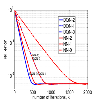
Refer to caption
Refer to caption
Figure 1: Relative error versus number of iterations k𝑘k (left) and versus number of communications (right) for quadratic costs and n=30𝑛30n=30-node network.
Refer to caption
Refer to caption
Figure 2: Relative error versus number of iterations k𝑘k (left) and versus number of communications (right) for quadratic costs and n=400𝑛400n=400-node network.

Figure 3 plots the relative error versus number of iterations (left) and number of per-node communications (right) for the logistic losses with variable dimension p=4𝑝4p=4 and the network with n=30𝑛30n=30 nodes. One can see that again the proposed methods perform better than the NN-\ell counterparts. In terms of the communication cost, DQN-00 is the most efficient among all methods, while DQN-222 is fastest in terms of the number of iterations. Finally, Figure 4 repeats the plots for variable dimension p=4𝑝4p=4 and the network with n=200𝑛200n=200 nodes, and it shows similar conclusions: among all DQN and NN methods, DQN-00 is the most efficient in terms of communications, while DQN-222 is fastest in terms of the number of iterations.
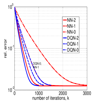
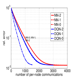
Refer to caption
Refer to caption
Figure 3: Relative error versus number of iterations k𝑘k (left) and versus number of communications (right) for logistic costs and n=30𝑛30n=30-node network.
Refer to caption
Refer to caption
Figure 4: Relative error versus number of iterations k𝑘k (left) and versus number of communications (right) for logistic costs and n=200𝑛200n=200-node network.

6 Extensions

As noted before, DQN methods do not converge to the exact solution of (1) but to a solution neighborhood controlled by the step size α𝛼\alpha. As such, for high solution accuracies required, they may not be competitive with distributed second order methods which converge to the exact solution [28, 38, 27].

However, we can exploit the results of [28] and “embed” the DQN algorithms in the framework of proximal multiplier methods (PMMs), just like [28] embeds the NN methods into the PMM framework. We refer to the resulting algorithms as PMM-DQN-\ell, =0,1,2.012\ell=0,1,2. (Here, PMM-DQN-\ell parallels DQN-\ell in terms of complexity of approximating Hessians, and in terms of the communication cost per iteration.) It is worth noting that the contribution to embed distributed second order methods into the PMM framework is due [28]. Here we extend [28] to demonstrate (by simulation) that the DQN-type Hessian approximations within the PMM framework yield efficient distributed second order methods.

We now briefly describe a general PMM-DQN method; for the methodology to devise distributed second order PMM methods, we refer to [28]. See also the Appendix for further details. We denote by x^k=(x^1k,,x^nk)npsuperscript^𝑥𝑘subscriptsuperscript^𝑥𝑘1subscriptsuperscript^𝑥𝑘𝑛superscript𝑛𝑝\mathaccent 866{x}^{\,k}=\left(\mathaccent 866{x}^{\,k}_{1},...,\mathaccent 866{x}^{\,k}_{n}\right)\in{\mathbb{R}}^{np} the current iterate, where x^ikpsubscriptsuperscript^𝑥𝑘𝑖superscript𝑝\mathaccent 866{x}^{\,k}_{i}\in{\mathbb{R}}^{p} is node i𝑖i’s estimate of the solution to (1) at iteration k𝑘k. Besides x^ksuperscript^𝑥𝑘\mathaccent 866{x}^{\,k} (the primal variable), the PMM-DQN method also maintains a dual variable q^k=(q^1k,,q^nk)npsuperscript^𝑞𝑘subscriptsuperscript^𝑞𝑘1subscriptsuperscript^𝑞𝑘𝑛superscript𝑛𝑝\mathaccent 866{q}^{\,k}=\left(\mathaccent 866{q}^{\,k}_{1},...,\mathaccent 866{q}^{\,k}_{n}\right)\in{\mathbb{R}}^{n\,p}, where q^ikpsubscriptsuperscript^𝑞𝑘𝑖superscript𝑝\mathaccent 866{q}^{\,k}_{i}\in{\mathbb{R}}^{p} is node i𝑖i’s dual variable at iteration k𝑘k. Quantities ^ksubscript^𝑘\mathaccent 866{\mathbb{H}}_{k}, 𝔸^ksubscript^𝔸𝑘\mathaccent 866{\mathbb{A}}_{k}, 𝔾^^𝔾\mathaccent 866{\mathbb{G}} and g^ksubscript^𝑔𝑘\mathaccent 866{g}_{k} defined below play a role in the PMM-DQN method and are, respectively, the counterparts of 2Φ(xk)superscript2Φsuperscript𝑥𝑘\nabla^{2}\Phi(x^{\,k}), 𝔸ksubscript𝔸𝑘{\mathbb{A}}_{k}, 𝔾𝔾{\mathbb{G}} and Φ(xk)Φsuperscript𝑥𝑘\nabla\Phi(x^{\,k}) with DQN:

^ksubscript^𝑘\displaystyle\mathaccent 866{\mathbb{H}}_{k} =\displaystyle= 2F(x^k)+β(𝕀)+ϵpmm𝕀=𝔸^k𝔾^superscript2𝐹superscript^𝑥𝑘𝛽𝕀subscriptitalic-ϵpmm𝕀subscript^𝔸𝑘^𝔾\displaystyle\nabla^{2}F(\mathaccent 866{x}^{\,k})+\beta\,\left(\mathbb{I}-\mathbb{Z}\right)+\epsilon_{\mathrm{pmm}}\,\mathbb{I}=\mathaccent 866{\mathbb{A}}_{k}-\mathaccent 866{\mathbb{G}} (51)
𝔸^ksubscript^𝔸𝑘\displaystyle\mathaccent 866{\mathbb{A}}_{k} =\displaystyle= 2F(x^k)+β(𝕀d)+ϵpmm𝕀+βθ(𝕀d)superscript2𝐹superscript^𝑥𝑘𝛽𝕀subscript𝑑subscriptitalic-ϵpmm𝕀𝛽𝜃𝕀subscript𝑑\displaystyle\nabla^{2}F(\mathaccent 866{x}^{\,k})+\beta\,\left(\mathbb{I}-{\mathbb{Z}}_{d}\right)+\epsilon_{\mathrm{pmm}}\,\mathbb{I}+\beta\,\theta\left(\mathbb{I}-\mathbb{Z}_{d}\right) (52)
𝔾^^𝔾\displaystyle\mathaccent 866{\mathbb{G}} =\displaystyle= βu+βθ(𝕀d)𝛽subscript𝑢𝛽𝜃𝕀subscript𝑑\displaystyle\beta\,{\mathbb{Z}}_{u}+\beta\,\theta\,\left(\mathbb{I}-\mathbb{Z}_{d}\right) (53)
g^ksubscript^𝑔𝑘\displaystyle\mathaccent 866{g}_{k} =\displaystyle= F(x^k)+β(𝕀)x^k+q^k.𝐹superscript^𝑥𝑘𝛽𝕀superscript^𝑥𝑘superscript^𝑞𝑘\displaystyle\nabla F(\mathaccent 866{x}^{\,k})+\beta\,(\mathbb{I}-\mathbb{Z})\mathaccent 866{x}^{\,k}+\mathaccent 866{q}^{\,k}. (54)

Here, θ0𝜃0\theta\geq 0 is the splitting parameter as with DQN, β>0𝛽0\beta>0 is the dual step size and ϵpmm>0subscriptitalic-ϵpmm0\epsilon_{\mathrm{pmm}}>0 relates to the proximal term of the corresponding augmented Lagrangian; see [28] for details. We now present the general PMM-DQN algorithm. Note from Step 2 the analogous form of the Hessian inverse approximation as with DQN; the approximation is again parameterized with a (np)×(np)𝑛𝑝𝑛𝑝(np)\times(np) diagonal matrix 𝕃^k.subscript^𝕃𝑘\mathaccent 866{\mathbb{L}}_{k}.

Algorithm 4: PMM-DQN in vector format
Given x0=0superscript𝑥00x^{0}=0, β,ϵpmm,ρ>0,θ0formulae-sequence𝛽subscriptitalic-ϵpmm𝜌0𝜃0\beta,\epsilon_{\mathrm{pmm}},\rho>0,\;\theta\geq 0. Set k=0.𝑘0k=0.

  • Step 1.

    Chose a diagonal matrix 𝕃^knp×npsubscript^𝕃𝑘superscript𝑛𝑝𝑛𝑝\mathaccent 866{\mathbb{L}}_{k}\in\mathbb{R}^{np\times np} such that

    𝕃^kρ.normsubscript^𝕃𝑘𝜌\|\mathaccent 866{\mathbb{L}}_{k}\|\leq\rho.
  • Step 2.

    Set

    s^k=(𝕀𝕃^k𝔾^)𝔸^k1g^k.superscript^𝑠𝑘𝕀subscript^𝕃𝑘^𝔾superscriptsubscript^𝔸𝑘1subscript^𝑔𝑘\mathaccent 866{s}^{\,k}=-(\mathbb{I}-\mathaccent 866{\mathbb{L}}_{k}\mathaccent 866{\mathbb{G}})\mathaccent 866{{\mathbb{A}}}_{k}^{-1}\,\mathaccent 866{g}_{k}.
  • Step 3.

    Set

    x^k+1=x^k+s^k.superscript^𝑥𝑘1superscript^𝑥𝑘superscript^𝑠𝑘\mathaccent 866{x}^{\,k+1}=\mathaccent 866{x}^{\,k}+\mathaccent 866{s}^{\,k}.
  • Step 4.

    Set

    q^k+1=q^k+(𝕀)x^k+1;k=k+1.formulae-sequencesuperscript^𝑞𝑘1superscript^𝑞𝑘𝕀superscript^𝑥𝑘1𝑘𝑘1\mathaccent 866{q}^{\,k+1}=\mathaccent 866{q}^{\,k}+\left(\mathbb{I}-\mathbb{Z}\right)\mathaccent 866{x}^{\,k+1};\;k=k+1.

The same algorithm is presented below from the distributed implementation perspective. (Note that here we adopt the notation similar to DQN, i.e., the (i,j)𝑖𝑗(i,j)-th p×p𝑝𝑝p\times p block of 𝔾^^𝔾\mathaccent 866{\mathbb{G}} is denoted by G^ijsubscript^𝐺𝑖𝑗\mathaccent 866{G}_{ij}; the i𝑖i-th p×p𝑝𝑝p\times p diagonal block of 𝕃^ksubscript^𝕃𝑘\mathaccent 866{\mathbb{L}}_{k} is denoted by Λ^iksubscriptsuperscript^Λ𝑘𝑖\mathaccent 866{\Lambda}^{\,k}_{i}; and i𝑖i-th p×p𝑝𝑝p\times p diagonal block of 𝔸^ksubscript^𝔸𝑘\mathaccent 866{\mathbb{A}}_{k} is denoted by A^iksubscriptsuperscript^𝐴𝑘𝑖\mathaccent 866{A}^{\,k}_{i}.)

Algorithm 5: PMM-DQN – Distributed implementation
At each node i𝑖i, require β,ρ,ϵpmm>0𝛽𝜌subscriptitalic-ϵpmm0\beta,\rho,\epsilon_{\mathrm{pmm}}>0, θ0𝜃0\theta\geq 0.

  • 1

    Initialization: Each node i𝑖i sets k=0𝑘0k=0 and x^i0=q^i0=0superscriptsubscript^𝑥𝑖0superscriptsubscript^𝑞𝑖00\mathaccent 866{x}_{i}^{0}=\mathaccent 866{q}_{i}^{0}=0.

  • 2

    Each node i𝑖i calculates

    d^ik=(A^ik)1[fi(x^ik)+βjOiwij(x^ikx^jk)+q^ik].superscriptsubscript^𝑑𝑖𝑘superscriptsuperscriptsubscript^𝐴𝑖𝑘1delimited-[]subscript𝑓𝑖superscriptsubscript^𝑥𝑖𝑘𝛽subscript𝑗subscript𝑂𝑖subscript𝑤𝑖𝑗superscriptsubscript^𝑥𝑖𝑘superscriptsubscript^𝑥𝑗𝑘superscriptsubscript^𝑞𝑖𝑘\mathaccent 866{d}_{i}^{\,k}=\left(\mathaccent 866{A}_{i}^{\,k}\right)^{-1}\left[\,\nabla f_{i}(\mathaccent 866{x}_{i}^{\,k})+\beta\,\sum_{j\in O_{i}}w_{ij}\left(\mathaccent 866{x}_{i}^{\,k}-\mathaccent 866{x}_{j}^{\,k}\right)+\mathaccent 866{q}_{i}^{\,k}\,\right].
  • 3

    Each node i𝑖i transmits d^iksuperscriptsubscript^𝑑𝑖𝑘\mathaccent 866{d}_{i}^{\,k} to all its neighbors jOi𝑗subscript𝑂𝑖j\in O_{i} and receives d^jksuperscriptsubscript^𝑑𝑗𝑘\mathaccent 866{d}_{j}^{\,k} from all jOi𝑗subscript𝑂𝑖j\in O_{i}.

  • 4

    Each node i𝑖i chooses a diagonal p×p𝑝𝑝p\times p matrix Λ^iksuperscriptsubscript^Λ𝑖𝑘\mathaccent 866{\Lambda}_{i}^{\,k}, such that Λ^ikρ.normsuperscriptsubscript^Λ𝑖𝑘𝜌\|\mathaccent 866{\Lambda}_{i}^{\,k}\|\leq\rho.

  • 6

    Each node i𝑖i calculates:

    s^ik=d^ik+Λ^ikjO¯iG^ijd^jk.superscriptsubscript^𝑠𝑖𝑘superscriptsubscript^𝑑𝑖𝑘superscriptsubscript^Λ𝑖𝑘subscript𝑗subscript¯𝑂𝑖subscript^𝐺𝑖𝑗superscriptsubscript^𝑑𝑗𝑘\mathaccent 866{s}_{i}^{\,k}=-\mathaccent 866{d}_{i}^{\,k}+\mathaccent 866{\Lambda}_{i}^{\,k}\sum_{j\in\bar{O}_{i}}\mathaccent 866{G}_{ij}\,\mathaccent 866{d}_{j}^{\,k}.
  • 6

    Each node i𝑖i updates its solution estimate as:

    x^ik+1=x^ik+s^ik.superscriptsubscript^𝑥𝑖𝑘1superscriptsubscript^𝑥𝑖𝑘superscriptsubscript^𝑠𝑖𝑘\mathaccent 866{x}_{i}^{\,k+1}=\mathaccent 866{x}_{i}^{\,k}+\mathaccent 866{s}_{i}^{\,k}.
  • 7

    Each node i𝑖i transmits x^ik+1superscriptsubscript^𝑥𝑖𝑘1\mathaccent 866{x}_{i}^{\,k+1} to all its neighbors jOi𝑗subscript𝑂𝑖j\in O_{i} and receives x^jk+1superscriptsubscript^𝑥𝑗𝑘1\mathaccent 866{x}_{j}^{\,k+1} from all jOi𝑗subscript𝑂𝑖j\in O_{i}.

  • 8

    Each node i𝑖i updates the dual variable q^iksuperscriptsubscript^𝑞𝑖𝑘\mathaccent 866{q}_{i}^{k} as follows:

    q^ik+1=q^ik+jOiwij(x^ik+1x^jk+1).superscriptsubscript^𝑞𝑖𝑘1superscriptsubscript^𝑞𝑖𝑘subscript𝑗subscript𝑂𝑖subscript𝑤𝑖𝑗superscriptsubscript^𝑥𝑖𝑘1superscriptsubscript^𝑥𝑗𝑘1\mathaccent 866{q}_{i}^{\,k+1}=\mathaccent 866{q}_{i}^{\,k}+\sum_{j\in O_{i}}w_{ij}\left(\mathaccent 866{x}_{i}^{\,k+1}-\mathaccent 866{x}_{j}^{\,k+1}\right).
  • 9

    Set k=k+1𝑘𝑘1k=k+1 and go to Step 2.

Note that, at Step 2, each node i𝑖i needs the neighbors’ estimates x^jksuperscriptsubscript^𝑥𝑗𝑘\mathaccent 866{x}_{j}^{k}, jOi𝑗subscript𝑂𝑖j\in O_{i}. For k1𝑘1k\geq 1, the availability of such information is ensured through Step 7 of the previous iteration k1𝑘1k-1; at k=0𝑘0k=0, Step 2 is also realizable as it is assumed that x^i0=0superscriptsubscript^𝑥𝑖00\mathaccent 866{x}_{i}^{0}=0, for all i=1,,n𝑖1𝑛i=1,...,n. As with the DQN methods, different variants PMM-DQN-\ell mutually differ in the choice of matrix 𝕃^ksubscript^𝕃𝑘\mathaccent 866{\mathbb{L}}_{k}. With PMM-DQN-00, we set 𝕃^k=0subscript^𝕃𝑘0\mathaccent 866{\mathbb{L}}_{k}=0; with PMM-DQN-222, 𝕃^ksubscript^𝕃𝑘\mathaccent 866{\mathbb{L}}_{k} is set as described below; with PMM-DQN-111, we set 𝕃^k=𝕃^=constsubscript^𝕃𝑘^𝕃const\mathaccent 866{\mathbb{L}}_{k}=\mathaccent 866{\mathbb{L}}=\mathrm{const} to 𝕃^0subscript^𝕃0\mathaccent 866{\mathbb{L}}_{0}, i.e., to the value of 𝕃^ksubscript^𝕃𝑘\mathaccent 866{\mathbb{L}}_{k} from the first iteration of PMM-DQN-222.

We now detail how 𝕃^ksubscript^𝕃𝑘\mathaccent 866{\mathbb{L}}_{k} is chosen with PMM-DQN-222. The methodology is completely analogous to DQN-222: the idea is to approximate the exact Newton direction s^Nksuperscriptsubscript^𝑠𝑁𝑘\mathaccent 866{s}_{N}^{k} which obeys the following Newton-type equation:

^ks^k+g^k=0,subscript^𝑘superscript^𝑠𝑘subscript^𝑔𝑘0\mathaccent 866{\mathbb{H}}_{k}\,\mathaccent 866{s}^{\,k}+\mathaccent 866{g}_{k}=0, (55)

through Taylor expansions. Using (55) and completely analogous steps as with DQN-222, it follows that 𝕃^ksubscript^𝕃𝑘\mathaccent 866{\mathbb{L}}_{k} is obtained through solving the following system of linear equations with respect to 𝕃^ksubscript^𝕃𝑘\mathaccent 866{\mathbb{L}}_{k}:

𝕃^ku^k=(1β+ϵpmm𝕀+β(β+ϵpmm)21(β+ϵpmm)22F(x^k))u^ksubscript^𝕃𝑘superscript^𝑢𝑘1𝛽subscriptitalic-ϵpmm𝕀𝛽superscript𝛽subscriptitalic-ϵpmm21superscript𝛽subscriptitalic-ϵpmm2superscript2𝐹superscript^𝑥𝑘superscript^𝑢𝑘\displaystyle\mathaccent 866{\mathbb{L}}_{k}\,\mathaccent 866{u}^{\,k}=-\left(\frac{1}{\beta+\epsilon_{\mathrm{pmm}}}\mathbb{I}+\frac{\beta}{(\beta+\epsilon_{\mathrm{pmm}})^{2}}\mathbb{Z}-\frac{1}{(\beta+\epsilon_{\mathrm{pmm}})^{2}}\nabla^{2}F(\mathaccent 866{x}^{k})\right)\mathaccent 866{u}^{\,k} (56)
whereu^k=𝔾^𝔸^k1g^k.wheresuperscript^𝑢𝑘^𝔾superscriptsubscript^𝔸𝑘1subscript^𝑔𝑘\displaystyle\mathrm{where}\,\,\,\,\,\mathaccent 866{u}^{\,k}=\mathaccent 866{\mathbb{G}}\,{\mathaccent 866{\mathbb{A}}}_{k}^{\,-1}\,\mathaccent 866{g}_{k}.

The overall algorithm for setting 𝕃^ksubscript^𝕃𝑘\mathaccent 866{\mathbb{L}}_{k} with PMM-DQN-222 (step 4 of Algorithm 5) is presented below.

Algorithm 6: Computing 𝕃^ksubscript^𝕃𝑘\mathaccent 866{\mathbb{L}}_{k} with PMM-DQN-222

  • 4.1

    Each node i𝑖i calculates

    u^ik=jO¯iG^ijd^jk.superscriptsubscript^𝑢𝑖𝑘subscript𝑗subscript¯𝑂𝑖subscript^𝐺𝑖𝑗superscriptsubscript^𝑑𝑗𝑘\mathaccent 866{u}_{i}^{\,k}=\sum_{j\in\bar{O}_{i}}\mathaccent 866{G}_{ij}\,\mathaccent 866{d}_{j}^{\,k}.
  • 4.2

    Each node i𝑖i transmits u^iksuperscriptsubscript^𝑢𝑖𝑘\mathaccent 866{u}_{i}^{\,k} to all its neighbors jOi𝑗subscript𝑂𝑖j\in O_{i} and receives u^jksuperscriptsubscript^𝑢𝑗𝑘\mathaccent 866{u}_{j}^{\,k} from all jOi𝑗subscript𝑂𝑖j\in O_{i}.

  • 4.3

    Each node i𝑖i calculates Λ^iksuperscriptsubscript^Λ𝑖𝑘\mathaccent 866{\Lambda}_{i}^{\,k} – the solution to the following system of equations (where the only unknown is the p×p𝑝𝑝p\times p diagonal matrix Λ^isubscript^Λ𝑖\mathaccent 866{\Lambda}_{i}):

    Λ^iu^ik=[(1β+ϵpmm+βwii(β+ϵpmm)2)I1(β+ϵpmm)22fi(x^ik)]subscript^Λ𝑖superscriptsubscript^𝑢𝑖𝑘delimited-[]1𝛽subscriptitalic-ϵpmm𝛽subscript𝑤𝑖𝑖superscript𝛽subscriptitalic-ϵpmm2𝐼1superscript𝛽subscriptitalic-ϵpmm2superscript2subscript𝑓𝑖superscriptsubscript^𝑥𝑖𝑘\displaystyle\mathaccent 866{\Lambda}_{i}\,\mathaccent 866{u}_{i}^{\,k}=-\left[\,(\frac{1}{\beta+\epsilon_{\mathrm{pmm}}}+\frac{\beta\,w_{ii}}{(\beta+\epsilon_{\mathrm{pmm}})^{2}})I-\frac{1}{(\beta+\epsilon_{\mathrm{pmm}})^{2}}\nabla^{2}f_{i}(\mathaccent 866{x}_{i}^{\,k})\,\right]
    ×u^ikβ(β+ϵpmm)2jOiwiju^jk.absentsuperscriptsubscript^𝑢𝑖𝑘𝛽superscript𝛽subscriptitalic-ϵpmm2subscript𝑗subscript𝑂𝑖subscript𝑤𝑖𝑗superscriptsubscript^𝑢𝑗𝑘\displaystyle\phantom{\Lambda_{i}\,\mathaccent 866{u}_{i}^{\,k}=}\times\mathaccent 866{u}_{i}^{\,k}-\frac{\beta}{(\beta+\epsilon_{\mathrm{pmm}})^{2}}\sum_{j\in O_{i}}w_{ij}\,\mathaccent 866{u}_{j}^{\,k}.
  • 4.4

    Each node i𝑖i projects each diagonal entry of Λ^iksuperscriptsubscript^Λ𝑖𝑘\mathaccent 866{\Lambda}_{i}^{k} onto the interval [ρ,ρ]𝜌𝜌[-\rho,\,\rho].

Simulations. We now compare by simulation the PMM-DQN-\ell methods with the ESOM-\ell algorithms proposed in [28], the DQM algorithm in [27], and different variants of the Newton Raphson Consensus (NRC) algorithm proposed in [38].

The simulation setup is as follows. The network is an instance of the random geometric graph with n=30𝑛30n=30 nodes and 166166166 links. The optimization variable dimension is p=4𝑝4p=4, and the local nodes costs are strongly convex quadratic, generated at random in the same way as with the quadratic costs examples in Section 5. With all methods which involve weighted averaging (ESOM-\ell, PMM-DQN-\ell, and NRC), we use the Metropolis weights. We consider the ESOM-\ell and PMM-DQN-\ell methods for =0,1,2.012\ell=0,1,2. With the methods ESOM-\ell and PMM-DQN-\ell, we set the proximal constant ϵpmm=10subscriptitalic-ϵpmm10\epsilon_{\mathrm{pmm}}=10 (see [28] for details). Further, we tune the dual step size β𝛽\beta separately for each of these methods to the best by considering the following candidate values: β{104,103.5,103,,103.5,104}𝛽superscript104superscript103.5superscript103superscript103.5superscript104\beta\in\{10^{-4},10^{-3.5},10^{-3},...,10^{3.5},10^{4}\}, i.e., a grid of points equidistant on the log10subscriptlog10\mathrm{log}_{10} scale with the half-decade spacing. The algorithm DQM has the tuning step size parameter c>0𝑐0c>0 (see [27] for details) which we also tune to the best using the same grid of candidate values. Regrading the methods proposed in [38], we consider both the standard (NRC) and the accelerated (FNRC) algorithm variant. These methods have a communication cost per node, per iteration which is quadratic in p𝑝p, due to exchanging local Hessian estimates. (Specifically, as it is sufficient to transmit the upper-triangular part of a local Hessian (due to the matrix symmetry), each node per iteration transmits p×(p+1)/2𝑝𝑝12p\times(p+1)/2 scalars for the Hessian exchange.) This is different from the ESOM, DQM, and PMM-DQN methods which have a cost linear in p𝑝p. We also consider the Jacobi variants in [38] (both the standard – JC and the accelerated – FJC variant) which approximate local Hessians through diagonal matrices and hence their communication cost per node, per iteration reduces to a cost linear in p𝑝p. With NRC, FNRC, JC, and FJC, we set their step size ϵitalic-ϵ\epsilon to unity (see [38] for details), as this (maximal possible) step size value yielded fastest convergence. We observed that JC and FJC converged with a non-zero limiting error, while decreasing the value of ϵitalic-ϵ\epsilon did not improve the limiting error of the method while slowing down the methods. Hence, with all the methods considered, we tune their step sizes to the best (up to the finite candidate grid points resolution). With FNRC and FJC, we set the acceleration parameter ϕitalic-ϕ\phi in the same way as in [38] (see page 10 of [38].) With all PMM-DQN methods, we do not use safeguarding (ρ=+𝜌\rho=+\infty), and we set θ=0𝜃0\theta=0. With all the methods considered, the primal variables – solution estimates (and dual variables, if exist) are initialized with zero vectors. The error metric is the same as with the quadratic example in Section 5.

Figure 5 compares the PMM-DQN-\ell algorithms and the ESOM-\ell algorithms in [28] in terms of the number of iterations (left) and the number of per-node communications (right). We can see that, in terms of iterations, for each fixed \ell, the corresponding PMM-DQN method performs better than the corresponding ESOM method. The exception is the case =00\ell=0 where the two methods are comparable. The same conclusions hold for the number of communications also. Further, in terms of the number of iterations, PMM-DQN-1 and PMM-DQN-2 are the best among all methods; in terms of communications, PMM-DQN-1 is the best method among all PMM-DQN and ESOM method considered.

In Figure 6, we compare the best among the PMM-DQN-\ell methods, the best among the ESOM-\ell methods (in terms of iterations, the best are PMM-DQN-1 and ESOM-2, while in terms of communications, the best are PMM-DQN-1 and ESOM-0), DQM, and the NRC methods group (NRC, FNRC, JC, and FJC). We can see that the PMM-DQN-1 method converges faster than all other methods, both in terms of iterations and communications.
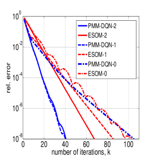
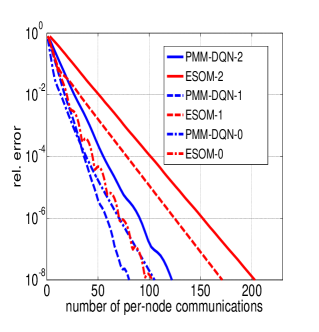
Refer to caption
Refer to caption
Figure 5: Comparison between the PMM-DQN-\ell algorithms and the ESOM-\ell algorithms in [28]. The figures plot relative error versus number of iterations k𝑘k (left) and versus number of communications (right) for quadratic costs and n=30𝑛30n=30-node network.
Refer to caption
Refer to caption
Figure 6: Comparison between the DQM algorithm in [27], the NRC algorithm in [38], the best among the PMM-DQN-\ell algorithms, and the best among the ESOM-\ell algorithms. The Figures plot relative error versus number of iterations k𝑘k (left) and versus number of communications (right) for quadratic costs and n=30𝑛30n=30-node network.

7 Conclusions

The problem under consideration is defined by an aggregate, network-wide sum cost function across nodes in a connected network. It is assumed that the cost functions are convex and differentiable, while the network is characterized by a symmetric, stochastic matrix W𝑊W that fulfils standard assumptions. The proposed methods are designed by exploiting a penalty reformulation of the original problem and rely heavily on the sparsity structure of the Hessian. The general method is tailored as a Newton-like method, taking the block diagonal part of the Hessian as an approximate Hessian and then correcting this approximation by a diagonal matrix 𝕃ksubscript𝕃𝑘\mathbb{L}_{k}. The key point in the proposed class of methods is to exploit the structure of Hessian and replace the dense part of the inverse Hessian by an inexpensive linear approximation, determined by matrix 𝕃ksubscript𝕃𝑘\mathbb{L}_{k}. Depending on the choice of 𝕃ksubscript𝕃𝑘\mathbb{L}_{k}, one can define different methods, and three of such choices are analyzed in this work. An important characteristic of the whole class of DQN methods is global linear convergence with a proper choice of the step size. Furthermore, we have shown local linear convergence for the full step size using the convergence theory of Inexact Newton methods as well as global convergence with the full step size for the special case of strictly convex quadratic loss functions.

The three specific methods are analyzed in detail, termed DQN-0, DQN-1 and DQN-2. They are defined by the three different choices of matrix 𝕃ksubscript𝕃𝑘\mathbb{L}_{k} – the zero matrix, a constant matrix, and the iteration-varying matrix that defines a search direction which mimics the Newton direction as much as possible under the imposed restrictions of inexpensive distributed implementation. For the last choice of the time varying matrix, we have shown local linear convergence for the full step size without safeguarding.

The cost in terms of computational effort and communication of these three methods correspond to the costs of the state-of-the-art Network Newton methods, NN-0, NN-1 and NN-2, which are used as the benchmark class in this paper. The simulation results on two relevant problems, the quadratic loss and the logistic loss, demonstrate the efficiency of the proposed methods and compare favorably with the benchmark methods. Finally, applying the recent contributions of [28], the proposed distributed second order methods were extended to the framework of proximal multiplier methods. Unlike DQN, the modified methods converge to the exact solution and further enhance the performance when high solution accuracies are required.

Acknowledgement. We are grateful to the anonymous referees whose comments and suggestions helped us to improve the quality of this paper.

References

  • [1] Boyd, S., Parikh, N., Chu, E., Peleato, B., Eckstein, J., Distributed optimization and statistical learning via the alternating direction method of multipliers, Foundations and Trends in Machine Learning, Volume 3, Issue 1, (2011) pp. 1-122.
  • [2] Byrd, R. H., Chin, G. M., Neveitt, W., Nocedal, J., On the Use of Stochastic Hessian Information in Optimization Methods for Machine Learning, SIAM Journal on Optimization, 21 (3), (2011) pp. 977-995.
  • [3] Byrd, R. H.. Chin, G. M., Nocedal, J., Wu, Y., Sample size selection in optimization methods for machine learning, Mathematical Programming, no. 134 vol. 1 (2012) pp. 127-155.
  • [4] Byrd, R. H., Hansen, S. L. , Nocedal, J., Singer, Y., A Stochastic Quasi-Newton Method for Large-Scale Optimization, SIAM J. Optimization, 26 (2) (2016) 1008-1031.
  • [5] Cattivelli, F., Sayed, A. H., Diffusion LMS strategies for distributed estimation, IEEE Transactions on Signal Processing, vol. 58, no. 3, (2010) pp. 1035–1048.
  • [6] Chen I.-A., Ozdaglar, A., A fast distributed proximal gradient method, in Allerton Conference on Communication, Control and Computing, Monticello, IL, October 2012.
  • [7] Daneshmand, A., Facchinei, F., Kungurtsev, V., Scutari, G., Hybrid random/deterministic parallel algorithms for nonconvex big data optimization, IEEE Transactions on Signal Processing, 63 (15) (2014), 3914-3929.
  • [8] Dembo, R.S. Eisenstat, S.C. Steinhaug, T., Inexact Newton method, SIAM Journall on Numerical Analysis 19,2, (1982), 400-409.
  • [9] Dennis, J.R., Schnabel R.B., Numerical Methods for Unconstrained Optimization and Nonlinear Equations (1996) SIAM
  • [10] Eisen, M., Mokhtari, A., Ribeiro, A., A Decentralized Quasi-Newton Method for Dual Formulations of Consensus Optimization, 2016, IEEE Conference on Decision and Control (CDC), to appear, 2016.
  • [11] Feingold, D.G., Varga, R. S., Block Diagonally Dominant Matrices and Generalizations of the Gershgorin Circle Theorem, Pacific Journal of Mathematics, 12 (4), (1962) 1241-1250.
  • [12] Friedlander, M. P. , Schmidt, M., Hybrid deterministic-stochastic methods for data fitting, SIAM Journal on Scientific Computing 34 (2012), 1380-1405.
  • [13] Jakovetić, D., Bajović, D., Krejić, N., Krklec Jerinkić, N., Distributed Gradient Methods with Variable Number of Working Nodes, IEEE Transactions on Signal Processing, 64 (15), (2016), 4080-4095.
  • [14] Jakovetić, D., Xavier, J., Moura, J. M. F., Fast distributed gradient methods, IEEE Transactions on Automatic Control, vol. 59, no. 5, (2014) pp. 1131–1146.
  • [15] Jakovetić, D., Moura, J. M. F., Xavier, J., Distributed Nesterov-like gradient algorithms, in CDC’12, 51stst{}^{\textrm{st}} IEEE Conference on Decision and Control, Maui, Hawaii, December 2012, pp. 5459–5464.
  • [16] Kar, S., Moura, J. M. F., Ramanan, K., Distributed parameter estimation in sensor networks: Nonlinear observation models and imperfect communication, IEEE Transactions on Information Theory, vol. 58, no. 6, (2012) pp. 3575–3605.
  • [17] Krejić, N., Krklec, N., Variable sample size methods for unconstrained optimization, Journal of Computational and Applied Mathematics 245 (2013), 213-231.
  • [18] Krejić, N., Krklec Jerinkić, N., Nonmonotone line search methods with variable sample size, Numerical Algorithms 68 (2015), pp. 711-739.
  • [19] Krejić N., Lužanin Z., Newton-like method with modification of the right-hand side vector, Mathematics of Computation, 71, 237 (2002), 237-250.
  • [20] Lobel, I., Ozdaglar, A., Feijer, D., Distributed Multi-agent Optimization with State-Dependent Communication, Mathematical Programming, vol. 129, no. 2, (2014) pp. 255-284.
  • [21] Lopes, C., Sayed, A. H., Adaptive estimation algorithms over distributed networks, in 21st IEICE Signal Processing Symposium, Kyoto, Japan, Nov. 2006.
  • [22] Mokhtari, A., Ling, Q., Ribeiro, A., An approximate Newton method for distributed optimization, Proc. Int. Conf. Acoustic Speech Signal Process pp. 2959-2963, Brisbane, Australia, 2015.
  • [23] Mokhtari, A., Ling, Q., Ribeiro, A., Network Newton–Part I: Algorithm and Convergence, 2015, available at: http://arxiv.org/abs/1504.06017
  • [24] Mokhtari, A., Ling, Q., Ribeiro, A., Network Newton–Part II: Convergence Rate and Implementation, 2015, available at: http://arxiv.org/abs/1504.06020
  • [25] Mokhtari, A., Ribeiro, A., Regularized Stochastic BFGS method, IEEE Transactions on Signal Processing, Vol. 62, no. 23, (2014) pp. 6089-6104.
  • [26] Mokhtari, A., Ribeiro, A., Global convergence of Online Limited Memory BFGS Method, J. Machine Learning Research, vol. 17 no. 61 (2016), 1-35.
  • [27] A. Mokhtari, W. Shi, Q. Ling, and A. Ribeiro, DQM: Decentralized Quadratically Approximated Alternating Direction Method of Multipliers, IEEE Trans. Sig. Process., vol. 64, no. 19 (2016), 5158-5173.
  • [28] A. Mokhtari, W. Shi, Q. Ling, and A. Ribeiro, A Decentralized Second Order Method with Exact Linear Convergence Rate for Consensus Optimization, IEEE Tran. Signal and Information Processing over Networks (to appear), 2016.
  • [29] Mota, J., Xavier, J., Aguiar, P., Püschel, M., Distributed optimization with local domains: Applications in MPC and network flows, IEEE Transactions on Automatic Control, vol. 60, no. 7 (2015), 2004-2009.
  • [30] Nedić, A., Ozdaglar, A., Distributed subgradient methods for multi-agent optimization, IEEE Transactions on Automatic Control, vol. 54, no. 1, (2009) pp. 48–61.
  • [31] Ram, S., Nedić, A., Veeravalli, V., Distributed stochastic subgradient projection algorithms for convex optimization, Journal on Optimization Theory and Applications, vol. 147, no. 3, (2011) pp. 516–545.
  • [32] Ram, S. S. , Nedić, A., Veeravalli, V., Asynchronous gossip algorithms for stochastic optimization, in CDC ’09, 48th IEEE International Conference on Decision and Control, Shanghai, China, December 2009, pp. 3581 – 3586.
  • [33] Schizas, I. D. , Ribeiro, A., Giannakis, G. B., Consensus in ad hoc WSNs with noisy links – Part I: Distributed estimation of deterministic signals, IEEE Transactions on Signal Processing, vol. 56, no. 1, (2009) pp. 350–364.
  • [34] Shi, G., Johansson, K. H., Finite-time and asymptotic convergence of distributed averaging and maximizing algorithms, 2012, available at: http://arxiv.org/pdf/1205.1733.pdf
  • [35] W. Shi, Q. Ling, K. Yuan, G. Wu, and W. Yin, On the Linear Convergence of the ADMM in Decentralized Consensus Optimization, IEEE Transactions on Signal Processing, vol. 62, no. 7 (2013).
  • [36] Shi, W., Ling, Q., Wu, G., Yin, W., EXTRA: an Exact First-Order Algorithm for Decentralized Consensus Optimization, SIAM Journal on Optimization, No. 25 vol. 2, (2015) pp. 944-966.
  • [37] Wei, E., Ozdaglar, A., Jadbabaie, A., A distributed Newton method for network utility maximization I: algorithm, IEEE Transactions on Automatic Control, vol. 58, no. 9, (2013) pp. 2162- 2175.
  • [38] Varagnolo, D., Zanella, F., Cenedese, A., Pillonetto, G., Schenato, L., Newton-Raphson Consensus for Distributed Convex Optimization, IEEE Trans. Aut. Contr., vol. 61, no. 4 (2016).
  • [39] Xiao, L., Boyd, S., Lall, S., A scheme for robust distributed sensor fusion based on average consensus, in IPSN ’05, Information Processing in Sensor Networks, Los Angeles, California, 2005, pp. 63–70.
  • [40] Yuan, L., Ling, Q., Yin, W., On the convergence of decentralized gradient descent, 2013, available at: http://arxiv.org/abs/1310.7063.
  • [41] Zargham, M., Ribeiro, A., Jadbabaie, A., Accelerated dual descent for constrained convex network flow optimization, Decision and Control (CDC), 2013 IEEE 52nd Annual Conference on, pp. 1037-1042, 2013.

Appendix

Following [28], we briefly explain how we derive the PMM-DQN methods. The starting point for PMM-DQN is the quadratically approximated PMM method, which takes the following form (see [28] for details and derivations):

x^k+1superscript^𝑥𝑘1\displaystyle\mathaccent 866{x}^{\,k+1} =\displaystyle= x^k^k1(F(x^k)+q^k+β(𝕀)x^k)superscript^𝑥𝑘superscriptsubscript^𝑘1𝐹superscript^𝑥𝑘superscript^𝑞𝑘𝛽𝕀superscript^𝑥𝑘\displaystyle\mathaccent 866{x}^{\,k}-\mathaccent 866{\mathbb{H}}_{k}^{\,-1}\left(\nabla F(\mathaccent 866{x}^{\,k})+\mathaccent 866{q}^{\,k}+\beta(\mathbb{I}-\mathbb{Z})\mathaccent 866{x}^{\,k}\right) (57)
q^k+1superscript^𝑞𝑘1\displaystyle\mathaccent 866{q}^{\,k+1} =\displaystyle= q^k+β(𝕀)x^k+1.superscript^𝑞𝑘𝛽𝕀superscript^𝑥𝑘1\displaystyle\mathaccent 866{q}^{\,k}+\beta(\mathbb{I}-\mathbb{Z})\mathaccent 866{x}^{\,k+1}. (58)

Here, β>0𝛽0\beta>0 is the (dual) step size, ^ksubscript^𝑘\mathaccent 866{\mathbb{H}}_{k} is given in (51), and x^knpsuperscript^𝑥𝑘superscript𝑛𝑝\mathaccent 866{x}^{\,k}\in{\mathbb{R}}^{np} and q^knpsuperscript^𝑞𝑘superscript𝑛𝑝\mathaccent 866{q}^{\,k}\in{\mathbb{R}}^{np} are respectively the primal and dual variables at iteration k=0,1,,𝑘01k=0,1,..., initialized by x^ 0=q^ 0=0.superscript^𝑥 0superscript^𝑞 00\mathaccent 866{x}^{\,0}=\mathaccent 866{q}^{\,0}=0.

The challenge for distributed implementation of (57)–(58) is that the inverse of ^ksubscript^𝑘\mathaccent 866{\mathbb{H}}_{k} does not respect the sparsity pattern of the network. The ESOM methods, proposed in [28], approximate the inverse of ^ksubscript^𝑘\mathaccent 866{\mathbb{H}}_{k} following the NN-type approximations [22]. Here, we extend such possibilities and approximate the inverse of ^ksubscript^𝑘\mathaccent 866{\mathbb{H}}_{k} through the DQN-type approximations. This is defined in (51)–(53) and Algorithm PMM-DQN in Section 6.

As noted, the matrix 𝕃k=0subscript𝕃𝑘0\mathbb{L}_{k}=0 with PMM-DQN-0, and it is 𝕃k=𝕃0=constsubscript𝕃𝑘subscript𝕃0const\mathbb{L}_{k}=\mathbb{L}_{0}=\mathrm{const} with PMM-DQN-1, where 𝕃0subscript𝕃0\mathbb{L}_{0} is the matrix from the first iteration of the DQN-2 method. It remains to derive 𝕃ksubscript𝕃𝑘\mathbb{L}_{k} for PMM-DQN-2, as it is given in Section 6. As noted in Section 6, we approximate the Newton equation in (55). The derivation steps are the same as with DQN-2, with the following identification: 2Φ(xk)superscript2Φsuperscript𝑥𝑘\nabla^{2}\Phi(x^{k}) in (34) is replaced with ^ksubscript^𝑘\mathaccent 866{\mathbb{H}}_{k} in (55), and Φ(xk)Φsuperscript𝑥𝑘\nabla\Phi(x^{k}) with g^ksuperscript^𝑔𝑘\mathaccent 866{g}^{\,k} in (55). Then, equation (37) with DQN-2 transforms into the following equation with PMM-DQN-2:

𝕃^ku^k=^k1u^k,subscript^𝕃𝑘superscript^𝑢𝑘superscriptsubscript^𝑘1superscript^𝑢𝑘\mathaccent 866{\mathbb{L}}_{k}\,\mathaccent 866{u}^{\,k}=-\mathaccent 866{\mathbb{H}}_{k}^{\,-1}\mathaccent 866{u}^{\,k}, (59)

where u^ksuperscript^𝑢𝑘\mathaccent 866{u}^{\,k} is given in (56). Finally, it remains to approximate ^k1superscriptsubscript^𝑘1\mathaccent 866{\mathbb{H}}_{k}^{\,-1} through a first order Taylor approximation, as follows:

^k1superscriptsubscript^𝑘1\displaystyle\mathaccent 866{\mathbb{H}}_{k}^{\,-1} =\displaystyle= [(β+ϵpmm)(𝕀(ββ+ϵpmm1β+ϵpmm2F(x^k)))]1superscriptdelimited-[]𝛽subscriptitalic-ϵpmm𝕀𝛽𝛽subscriptitalic-ϵpmm1𝛽subscriptitalic-ϵpmmsuperscript2𝐹superscript^𝑥𝑘1\displaystyle\left[\,\,(\beta+\epsilon_{\mathrm{pmm}})\left(\,\mathbb{I}-\left(\frac{\beta}{\beta+\epsilon_{\mathrm{pmm}}}\mathbb{Z}-\frac{1}{\beta+\epsilon_{\mathrm{pmm}}}\nabla^{2}F(\mathaccent 866{x}^{\,k})\right)\,\right)\,\,\right]^{-1}
\displaystyle\approx 1β+ϵpmm[𝕀+ββ+ϵpmm1β+ϵpmm2F(x^k)].1𝛽subscriptitalic-ϵpmmdelimited-[]𝕀𝛽𝛽subscriptitalic-ϵpmm1𝛽subscriptitalic-ϵpmmsuperscript2𝐹superscript^𝑥𝑘\displaystyle\frac{1}{\beta+\epsilon_{\mathrm{pmm}}}\left[\,\,\mathbb{I}+\frac{\beta}{\beta+\epsilon_{\mathrm{pmm}}}\mathbb{Z}-\frac{1}{\beta+\epsilon_{\mathrm{pmm}}}\nabla^{2}F(\mathaccent 866{x}^{\,k})\,\,\right].

The above Taylor approximation is well defined if the spectral radius of matrix (ββ+ϵpmm1β+ϵpmm2F(x^k))𝛽𝛽subscriptitalic-ϵpmm1𝛽subscriptitalic-ϵpmmsuperscript2𝐹superscript^𝑥𝑘\left(\frac{\beta}{\beta+\epsilon_{\mathrm{pmm}}}\mathbb{Z}-\frac{1}{\beta+\epsilon_{\mathrm{pmm}}}\nabla^{2}F(\mathaccent 866{x}^{\,k})\right) is strictly less than one. It is easy to verify that this will be the case if the (positive) parameters β𝛽\beta and ϵpmmsubscriptitalic-ϵpmm\epsilon_{\mathrm{pmm}} satisfy β>12max{0,Lϵpmm}𝛽120𝐿subscriptitalic-ϵpmm\beta>\frac{1}{2}\max\{0,L-\epsilon_{\mathrm{pmm}}\}.