HAMSI: A Parallel Incremental Optimization Algorithm Using Quadratic Approximations for Solving Partially Separable Problems

Abstract.

We propose HAMSI (Hessian Approximated Multiple Subsets Iteration), which is a provably convergent, second order incremental algorithm for solving large-scale partially separable optimization problems. The algorithm is based on a local quadratic approximation, and hence, allows incorporating curvature information to speed-up the convergence. HAMSI is inherently parallel and it scales nicely with the number of processors. Combined with techniques for effectively utilizing modern parallel computer architectures, we illustrate that the proposed method converges more rapidly than a parallel stochastic gradient descent when both methods are used to solve large-scale matrix factorization problems. This performance gain comes only at the expense of using memory that scales linearly with the total size of the optimization variables. We conclude that HAMSI may be considered as a viable alternative in many large scale problems, where first order methods based on variants of stochastic gradient descent are applicable.

1. Introduction

A vast variety of problems in machine learning are framed as unconstrained optimization problems of the form

(1) $$\min_{x}\sum_{i\in\mathcal{I}}f_{i}(x),$$

where $x$ is a vector of parameters and $f_{i}$ are a collection of functions that implicitly depend on an observed data set. Formally, each index $i$ in the set $\mathcal{I}$ corresponds to a single data item, and the number of additive terms in the overall objective scales with the size of the available data. A natural approach for solving the so called large scale problems (where the set $\mathcal{I}$ is large) is using parallel computation and a divide-and-conquer approach.

In an optimization context, divide-and-conquer provides an immediate solution to the so-called separable problems. One particular toy example of a separable problem is the following:

(2) $$\min_{x}\{f_{1}(x_{1},x_{2})+f_{2}(x_{3})+f_{3}(x_{4},x_{5},x_{6})\}.$$

Here, the parameter vector $x=(x_{1},\cdots,x_{6})$ is partitioned into $3$ blocks, denoted by ${\boldsymbol{\alpha}}_{1}=\{1,2\}$, ${\boldsymbol{\alpha}}_{2}=\{3\}$ and ${\boldsymbol{\alpha}}_{3}=\{4,5,6\}$ and each objective function $f_{i}$ depends only on $x_{{\boldsymbol{\alpha}}_{i}}$ for all $i\in\{1,2,3\}$. We denote the parameter index set as $\mathcal{J}$ and the function index set as $\mathcal{I}$; in this example, $\mathcal{J}=\{1,\cdots,6\}$ and $\mathcal{I}=\{1,2,3\}$. As individual terms are additive, and ${\boldsymbol{\alpha}}_{i}$ are mutually disjoint, each subproblem $\min_{x}f_{i}(x_{{\boldsymbol{\alpha}}_{i}})$ can be solved in parallel and the results can be combined.

However, there are many optimization problems of interest that are not separable, primary examples being various matrix decomposition or regression problems. Fortunately, such problems still have some inherent structure that can be exploited for parallel computation. As an example, consider a slightly different toy example

(3) $$\min_{x}\{f_{1}(x_{1},x_{2})+f_{2}(x_{2},x_{3},x_{4})+f_{3}(x_{4},x_{5},x_{6})\},$$

where the parameter vector $x$ is again partitioned into $3$ blocks, ${\boldsymbol{\alpha}}_{1}=\{1,2\}$, ${\boldsymbol{\alpha}}_{2}=\{2,3,4\}$ and ${\boldsymbol{\alpha}}_{3}=\{4,5,6\}$. Here, the blocks ${\boldsymbol{\alpha}}_{i}$ are no longer mutually disjoint but have relatively small intersections; for example variable $x_{2}$ is shared among terms $f_{1}$ and $f_{2}$, while $x_{4}$ is shared between $f_{2}$ and $f_{3}$. We refer to such an objective function as partially separable. Such problems can be conveniently visualized using a bipartite graph $\mathcal{G}$ – also widely known as a factor graph (Kschischang et al., 2001), albeit in the context of probabilistic inference. Here, the optimization variables $x_{j}$ and the individual objective function terms $f_{i}$ correspond to nodes, and ${\boldsymbol{\alpha}}_{i}$ sets refer to the existing edges (see Figure 1). The graph represents the relation $j\in{\boldsymbol{\alpha}}_{i}$; formally, we have $\mathcal{G}=(\mathcal{I},\mathcal{J},\mathcal{E})$ with the vertex sets $\mathcal{I},\mathcal{J}$ and the edge set $\mathcal{E}$ such that for $i\in\mathcal{I}$ and $j\in\mathcal{J}$, we have $\{i,j\}\in\mathcal{E}$ when $j\in{\boldsymbol{\alpha}}_{i}$.

Figure 1. A bipartite graph (factor graph) representation of the two toy problems described in the text. (Left) For the separable problem, the graph is disconnected and each subgraph corresponds to an independent problem and can be optimized in parallel. (Right) For partially separable problems, the graph is connected. We can render the graph disconnected by removing some function terms (black squares).

1.1. Problem Statement

In the subsequent part of this paper, we shall focus on the following optimization problem:

(4) $$\min_{x\in\mathbb{R}^{|\mathcal{J}|}}\sum_{i\in\mathcal{I}}f_{i}(x_{{\boldsymbol{\alpha}}_{i}}),$$

where each term $f_{i}:\mathbb{R}^{|\mathcal{J}|}\mapsto\mathbb{R}$ for $i\in\mathcal{I}$ of the overall objective function $f$ is a twice continuously differentiable function. The function index set $\mathcal{I}\equiv\{1,2,\cdots,|\mathcal{I}|\}$ has typically a very large cardinality $|\mathcal{I}|$, however, each term $f_{i}$ depends only on a small subset of the elements of $x$; that is, $f_{i}(x)\equiv f_{i}(x_{{\boldsymbol{\alpha}}_{i}})$. Here ${\boldsymbol{\alpha}}_{i}$ are index sets such that for all $i\in\mathcal{I}$, ${\boldsymbol{\alpha}}_{i}\subseteq\mathcal{J}$ where the function index set $\mathcal{J}\equiv\{1,2,\cdots,|\mathcal{J}|\}$. Each singleton $j\in\mathcal{J}$ corresponds to a unique component of vector $x$, denoted as $x_{j}$. Thus, if ${\boldsymbol{\alpha}}=\{j_{1},j_{2},\cdots,j_{A}\}$, we have a vector $x_{\boldsymbol{\alpha}}=(x_{j_{1}},x_{j_{1}},\cdots,x_{j_{A}})$.

There are various strategies for the optimization of partially separable objective functions. One approach is based on taking alternating steps, where one can select each coordinate $x_{j}$ in turns while regarding the remaining variables $x_{-j}$ as constant, and at each step solves a smaller optimization problem $\min_{x_{j}}f(x_{j},x_{-j})$. Alternating least squares, coordinate descent, or various message passing algorithms are examples of alternating approaches.

In this paper, we shall focus on a different strategy, where we select a collection of terms $f_{i}$ rather than individual variables $x_{i}$. Such methods are known under the name incremental methods; cf. (Bertsekas, 2011). At each iteration $\tau$, an incremental method selects only a small subset of the function terms $f_{i}$. That is, a subset $S^{(\tau)}$ is selected from the function indices such that $S^{(\tau)}\subset\mathcal{I}$. Then, the iterative algorithm takes a step towards the minimum of a proxy objective function, $\sum_{i\in S^{(\tau)}}f_{i}(x)$ (see Figure 2). While at each step $\tau$ a different proxy objective is used and the actual objective is never evaluated, incremental algorithms still converge to a solution of the overall problem under mild conditions, with the stochastic gradient descent (SGD) being perhaps the most prominent example. In this paper, by careful selection of subsets $S^{(\tau)}$ at each step $\tau$, we shall keep the proxy objective separable to allow parallel computation.

Figure 2. Incremental optimization of a partially separable objective by two proxy objectives $f_{1}(x)+f_{3}(x)$ and $f_{2}(x)$. By only choosing a subset of the function terms (denoted by black squares) and omitting others (white squares) at each iteration we move towards the solution of the proxy objective. If the function terms are carefully selected, each proxy objective admits parallel optimization and by suitably damping the iterations, an approximate solution to the true solution can be obtained. We develop a general second order method for this general schema.

1.2. A Motivating Example

The rather generic form of the objective function given by (4) covers various optimization problems arising in machine learning. We provide here a particular example to demonstrate the general approach, yet the formulation can be applied to many other models and to a wide extent of the application areas. It can be easily checked, that problems such as sparse logical regression, matrix completion or multilayer perceptron training can be framed as solving a partially separable objective function of the form (4) expressable by a sparse factor graph.

Example 1.1.

Consider the following matrix factorization problem:

$$\min_{x}\left\|\left(\begin{array}[]{cc}y_{1}&y_{2}\\ y_{3}&y_{4}\\ y_{5}&y_{6}\end{array}\right)-\left(\begin{array}[]{c}x_{1}\\ x_{2}\\ x_{3}\end{array}\right)\left(\begin{array}[]{cc}x_{4}&x_{5}\\ \end{array}\right)\right\|_{F}^{2},$$

where $\|\cdot\|_{F}$ is the Frobenius norm. Then using our notation, the objective function becomes

$$\sum_{i\in\mathcal{I}}f_{i}(x_{{\boldsymbol{\alpha}}_{i}})=(y_{1}-x_{1}x_{4})^{2}+(y_{2}-x_{1}x_{5})^{2}+\cdots+(y_{6}-x_{3}x_{5})^{2}.$$

Clearly, we have $\mathcal{I}=\{1,2,\cdots,6\}$ and $\mathcal{J}=\{1,2,\cdots,5\}$ with the subsets ${\boldsymbol{\alpha}}_{1}=\{1,4\}$, ${\boldsymbol{\alpha}}_{2}=\{1,5\}$, ${\boldsymbol{\alpha}}_{3}=\{2,4\}$, ${\boldsymbol{\alpha}}_{4}=\{2,5\}$, ${\boldsymbol{\alpha}}_{5}=\{3,4\}$, and ${\boldsymbol{\alpha}}_{6}=\{3,5\}$. The corresponding bipartite graph is illustrated in Figure 3, left.

For a more general matrix factorization problem, we have an observed data matrix $Y\in\mathbb{R}^{K\times N}$ and we wish to find two factor matrices $X_{1}$ and $X_{2}$, where $X_{1}\in\mathbb{R}^{K\times L}$ and $X_{2}\in\mathbb{R}^{L\times N}$ such that

$$\min_{X_{1},X_{2}}\|Y-X_{1}X_{2}\|_{F}^{2}.$$

In elementwise notation we have

(6) $$f(x)=\sum_{a,b}(y_{a,b}-\sum_{k}x_{1,a,k}x_{2,k,b})^{2}.$$

Letting $i=(a,b)$, we see that this objective can be written as

$$f(x)=\sum_{i\in\mathcal{I}}f_{i}(x_{{\boldsymbol{\alpha}}_{i}}),$$

where ${\boldsymbol{\alpha}}_{i}$ is the set of indices that correspond to the row $a$ of $X_{1}$ and column $b$ of $X_{2}$. When some entries of the matrix $Y$ are unknown, the summation in Eq.6 is merely over the observed pairs $(a,b)$, leading still to the form of the final objective.

1.3. Related Literature

We propose an incremental and parallel algorithm that incorporates (approximate) curvature information for distributed large-scale optimization. Our experience confirms that using second order information can accelarate convergence even with incremental gradients. To gather second order information, the inner problems of our algorithm are modeled by quadratic functions. Similar to incremental and aggregate methods (Bertsekas, 2011; Tseng, 1998; Solodov, 1998; Blatt et al., 2007; Roux et al., 2012), our algorithm exploits the structure of the objective function, as characterized conveniently by the bipartite graph $\mathcal{G}$, and evaluates the gradient only for a subset of the component functions at each iteration, and it chooses the subsets of component functions in a way that provides separability of the inner problems. This helps to distribute the computations over multiple processors and enables doing stepwise computations on subdomains in parallel. Consequently, modern distributed and multicore computer systems can be easily utilized.

Gemulla et al. (2011) have proposed such a distribution scheme for the matrix factorization problem, which is employed to deal with large-scale distibuted relational data thanks to its partially-separable nature (Singh and Gordon, 2008; Cichocki et al., 2009). They employ SGD and analyze its convergence properties. They also consider the distribution of the problem data on a cluster of computers. The idea of second order incremental methods has also been investigated. Bertsekas (1996) has introduced such a method specifically designed for the least squares problem. His proposal is an incremental version of the Gauss-Newton method. An extension of this method for general functions has recently been presented by Gürbüzbalaban et al. (2014). They have shown linear convergence for the method under strong convexity and gradient growth assumptions. Moreover, their method requires the computation and the inversion of the exact Hessian matrices of the component functions. Shamir et al. (2014) have proposed a distributed Newton-like algorithm for convex problems, where the method requires to compute and invert $|{\mathcal{}J}|\times|{\mathcal{}J}|$ Hessian matrices that are local to each computational node. Due to its generic setting, the method cannot make use of an explicit parameter space decomposition, hence requires the entire parameter vector to be stored in the memory and communicated at every iteration. In another study, an incremental aggregated quasi-Newton algorithm has been proposed, where the main idea is to update the quadratic model of one component function at each iteration (Sohl-Dickstein et al., 2014).

Another group of recent work is devoted to stochastic quasi-Newton methods. The stochastic block BFGS approach proposed by Gower et al. (2016) does multi-secant updates, and employs variance-reduced gradients to achieve linear convergence for convex problems. In a recent study, Moritz et al. (2015) have proposed stochastic quasi-Newton methods that can achieve linear convergence rates under convexity assumptions, using aggregated gradients and variance reduction techniques. Whilst these methods have been shown to be useful in certain applications, they are not suitable for parallel computation due to their gradient aggregation steps. On the other hand, applying a quasi-Newton method with stochastic (or incremental) gradients is not straightforward as it may cause a data consistency problem, which becomes more prominent in a parallel computation setting; cf. (Schraudolph et al., 2007; Byrd et al., 2016; Berahas et al., 2016).

The analysis presented in (Gürbüzbalaban et al., 2014) for second order incremental methods does not cover our deterministic algorithm as they assume convexity of the objective function. Our analysis follows the lines of the analysis in (Solodov, 1998) of incremental gradient algorithms for nonconvex problems, which does not directly apply to our case since it does not cover the incorporation of second order information. In a recent study, (Wang et al., 2014) have analyzed a framework for stochastic quasi-Newton methods, which applies to nonconvex stochastic optimization problems. Their analysis covers our stochastic algorithm considering (1) as an expected value expression with a discrete probability distribution.

In this paper, we make the following contributions:

• We propose a generic algorithm, which incorporates second order information. The proposed algorithm can be applied to a large-class of convex and nonconvex problems, such as; matrix-tensor factorization, regression, and neural network training.

• We demonstrate the convergence properties of our algorithm when the subset selection step is deterministic. To the best of our knowledge, a proof for such a deterministic algorithm has not been given before in the machine learning literature.

• We investigate several shared-memory parallelization techniques and propose a simple cache-friendly load balancing heuristic that can be used for stratification-based parallel matrix and tensor processing. This latter contribution is particularly important in real applications, where the pattern of observed entries in a matrix or tensor is far from being uniformly distributed.

• To present a particular application of the generic algorithm, we give an implementation based on L-BFGS (Byrd et al., 1994) procedure, where we pay special attention to the consistency of the updates.

• We test our algorithm on large-scale matrix factorization problems of varying sizes and obtain faster convergence with superior solution times than a well-known first order method (Gemulla et al., 2011).

• Our implementation is available online, where interested readers can reproduce the results with the best performing algorithm in this paper. On the same page, we also report our results with the well-known MovieLens datasets. Our results are among the best ones to this date.

2. Proposed Algorithm: HAMSI

The gist of our approach is iterating over multiple subsets of data, where at each iteration a second order method can be employed. To derive the generic algorithm, let us first express the function index set $\mathcal{I}$ by a union of subsets $S_{k}$ for $k=1\cdots K$ such that

$$\mathcal{I}=S_{1}\cup\cdots\cup S_{k}\cup\cdots\cup S_{K}.$$

The subsets $S_{k}$ are not necessary mutually disjoint, but we typically choose them as such. We will refer to this collection of subsets a cover, that will be denoted as $\mathcal{S}\equiv\{S_{1},\cdots,S_{K}\}$. Furthermore, each subset $S_{k}\in\mathcal{S}$ for $k=1\cdots K$ is further partitioned into mutually exclusive blocks $B_{k}$ as

$$S_{k}=S_{k,1}\cup\cdots\cup S_{k,b}\cup\cdots\cup S_{k,B_{k}},$$

where $S_{k,b}\cap S_{k,b^{\prime}}=\emptyset$ for all $k$ and $b\neq b^{\prime}$. The example in Figure 2 has a partition

$$\mathcal{I}=S_{1}\cup S_{2}=(S_{1,1}\cup S_{1,2})\cup S_{2,1}=(\{1\}\cup\{3\})\cup\{2\}.$$

The cover $\mathcal{S}$ can be chosen in many ways. Once a cover is fixed, partitioning of each subset $S_{k}$ is guided by the factor graph, where the individual blocks correspond to the terms that can be independently optimized. This can be achieved by choosing the partitions $S_{k,b}$ such that the set of variable nodes connected to the function nodes $f_{i}$ such that $i\in S_{k,b}$ are mutually disjoint. Naturally, one can keep the number of blocks $B_{k}$ large to keep the degree of parallelism as high as possible.

The partitions can be understood easily by visualizing the bipartite graph. For the matrix factorization problem in Example 1.1, we have illustrated the partitioning in Figure 3. In a sense, we aim to solve the matrix factorization problem by approximately solving a sequence of matrix completion problems where the pattern of missing entries at each stage is carefully chosen by the algorithm.

Figure 3. (Left) The factor graph of the problem in Example 1.1. (Middle and Right) A partitioning of function index set as $\mathcal{I}=\cup_{k=1}^{K}S_{k}$ where $S_{k}=S_{k,1}\cup\cdots\cup S_{k,B_{k}}$ for $k=1\cdots K$. In this example $K=2$ and with number of blocks $B_{1}=B_{2}=2$. (Middle) First subset ($k=1$) with $S_{1}=S_{1,1}\cup S_{1,2}=\{1\}\cup\{4,6\}$ and ${\boldsymbol{\alpha}}_{1,1}=\{1,4\}$, ${\boldsymbol{\alpha}}_{1,2}=\{2,3,5\}$, (Right) Second subset ($k=2$) with $S_{2}=S_{2,1}\cup S_{2,2}=\{3,5\}\cup\{2\}$, ${\boldsymbol{\alpha}}_{k,1}=\{2,3,4\}$ and ${\boldsymbol{\alpha}}_{k,2}=\{1,5\}$. Note that each partition renders separable subproblems as the associated variable sets are mutually disjoint ${\boldsymbol{\alpha}}_{1,1}\cap{\boldsymbol{\alpha}}_{1,2}$ and ${\boldsymbol{\alpha}}_{2,1}\cap{\boldsymbol{\alpha}}_{2,2}$. The resulting algorithm can be viewed as alternating between two appropriately chosen matrix factorization problems with missing data, each of which can be solved efficiently in parallel by exploiting the separability.

Formally, we let

$$\mathcal{I}=\bigcup_{k=1}^{K}\bigcup_{b=1}^{B_{k}}S_{k,b},$$

where the optimization problem with a partially separable objective function (4) can be written as

(7) $$\min_{x\in\mathbb{R}^{|\mathcal{J}|}}\sum_{k=1}^{K}\sum_{b=1}^{B_{k}}\sum_{i\in S_{k,b}}f_{i}(x_{{\boldsymbol{\alpha}}_{i}}).$$

The parallelization within our algorithm relies on the fact that the objective function in (7) is separable over the second summation indexed by the block index $b$. To achieve this we define

$${\boldsymbol{\alpha}}_{k,b}\equiv\bigcup_{i\in S_{k,b}}{\boldsymbol{\alpha}}_{i}\ \ \mbox{ for all }k=1,\cdots,K;b=1,\cdots,B_{k},$$

and require $\ {\boldsymbol{\alpha}}_{k,b}\cap{\boldsymbol{\alpha}}_{k,b^{\prime}}=\emptyset\ \mbox{ for }b\neq b^{\prime}\mbox{ and }\ \bigcup_{b=1}^{B_{k}}{\boldsymbol{\alpha}}_{k,b}\subseteq\mathcal{J}\ \mbox{ for all }k=1,\cdots,K$. The equality $\ {\boldsymbol{\alpha}}_{k,b}\cap{\boldsymbol{\alpha}}_{k,b^{\prime}}=\emptyset$ is required for the parallel and exact computation of the (partial) gradients. However, as we describe in Section 5.2, there exist synchronization-free algorithms in the literature that accept a small amount of noise in the gradient. For these algorithms, the parameter sets of the blocks may be overlapping. In any case we have,

$$f_{k,b}(x_{{\boldsymbol{\alpha}}_{k,b}})=\sum_{i\in S_{k,b}}f_{i}(x_{\alpha_{i}}).$$

This construction leads to the final form of our optimization problem that we shall consider in our subsequent discussion:

(8) $$\min_{x\in\mathbb{R}^{|\mathcal{J}|}}\sum_{k=1}^{K}\sum_{b=1}^{B_{k}}f_{k,b}(x_{{\boldsymbol{\alpha}}_{k,b}}).$$

2.1. HAMSI

Our algorithm uses incremental gradients and incorporates a second order information into the optimization steps. The second order information comes from an approximation to the Hessian of the objective function. As we also work on multiple subsets of $|\mathcal{I}|$ functions, the algorithm is aptly called Hessian Approximated Multiple Subsets Iteration (HAMSI). The key idea of the algorithm is using a local convex quadratic approximation

(9) $$Q(z;\hat{x},g,H,\beta)\equiv(z-\hat{x})^{\top}g+\frac{1}{2}(z-\hat{x})^{\top}H(z-\hat{x})+\frac{1}{2}\beta\|z-\hat{x}\|^{2}$$

for step computation. Here, $g$ is an incremental gradient, $H$ is (an approximation to) the Hessian of the objective function. The parameter $\beta$ is crucial not only to bound the step length but also to control the oscillation of the incremental steps.

1 input : $x$, $H$, ${\boldsymbol{\alpha}}_{k,b}$ for all $k=1,\cdots,K$; $b=1,\cdots,B_{k}$.

2 $t=1$

3 ${\mathcal{K}}=[K,1,2,\cdots,K-1,K]$

4 repeat

5       Update $\beta_{t}$   (increasing sequence)

6       $\mathcal{K}\leftarrow$ SetSchedule($\mathcal{K}$)

7       for $\ell=1,2,\cdots,K+1$ do

8             $k={\mathcal{K}}[\ell]$

9             for $b=1,2,\cdots,B_{k}$ do in parallel

10                   $x_{{\boldsymbol{\alpha}}_{k,b}}=\mbox{arg min}_{z}Q(z;x_{{\boldsymbol{\alpha}}_{k,b}},\nabla f_{k,b}(x_{{\boldsymbol{\alpha}}_{k,b}}),H_{{\boldsymbol{\alpha}}_{k,b}},\beta_{t})$

11                  

12            

13      Evaluate approximate Hessian matrix $H$ at $x$

14       $t\leftarrow t+1$

15      

16until convergence or $t$ > max_epochs

Algorithm 1 Hessian Approximated Multiple Subsets Iteration (HAMSI)

Algorithm 1 gives the high-level pseudocode of HAMSI. In the algorithm, $x$ represents the current solution. At the $k^{th}$ inner iteration, HAMSI uses the functions in $S_{k}$ (lines 1-1). The order of the subsets, $\mathcal{K}$, is determined by a SetSchedule function which gets the current order as a parameter, obtains the new order by applying one cyclic left-shift to the first $K$ elements of $\mathcal{K}$ and makes sure that the sequence ends with the same number as the first. An illustrative execution of the SetSchedule function for $K=4$ is as follows:

Iteration $t$	$[3,4,1,2,3]=\text{\sc SetSchedule}([2,3,4,1,2])$
Iteration $t+1$	$[4,1,2,3,4]=\text{\sc SetSchedule}([3,4,1,2,3])$
Iteration $t+2$	$[1,2,3,4,1]=\text{\sc SetSchedule}([4,1,2,3,4])$
$\vdots$	$\vdots$

We note that the subsets are determined only once at the beginning and the SetSchedule function only reorders a schedule array $\mathcal{K}$ of size $K+1$ appropriately.

For each subset, lines 1 and 1 traverse the corresponding blocks and update the corresponding parts of the solution, where the updated part can be denoted as $\bigcup_{b=1}^{B_{k}}{\boldsymbol{\alpha}}_{k,b}$. It is important to note that the corresponding inner loop computes the blocks of each inner step in parallel and the same (approximate) matrix $H$ is employed at all inner iterations during the $t^{th}$ cycle. However, the inner iterations use different blocks of $H$ denoted by the submatrix $H_{{\boldsymbol{\alpha}}_{k,b}}$, where $H_{{\boldsymbol{\alpha}}}=\{H(i,i^{\prime}):i,i^{\prime}\in{\boldsymbol{\alpha}}\}$. The parameter $\beta_{t}$ is also constant during the inner iterations and then it is updated at the next iteration (line 1). The above description of the algorithm overlooks several important implementation details; in particular, how to construct the quadratic approximation in line 1 and how to solve the corresponding subproblems. We shall give an explicit implementation in Section 4, where we exemplify these details.

2.2. Convergence

Next, we show the convergence properties of HAMSI when the order of subset selection is deterministic. Our demonstration follows a similar construction as given in (Mangasarian and Solodov, 1994; Solodov, 1998). To simplify our exposition, we define

$$\nabla f_{S_{k}}(x)\equiv\sum_{b=1}^{B_{k}}\nabla f_{k,b}(x_{{\boldsymbol{\alpha}}_{k,b}})$$

and denote the solution at iteration $t$ by $x^{(t)}$. Since the approximate Hessian is also evaluated at $x^{(t)}$, we denote it by $H^{(t)}$. Notice that we update the current solution in lines 1-1. Thus, we denote those inner iterates by $x^{(t,\ell)}$. Using this notation, the very last inner iterate $x^{(t,K+1)}$ becomes $x^{(t+1)}$ after line 1.

Before presenting our results, let us first list our assumptions:

1. The twice differentiable objective function $f$ is bounded below.

2. The Hessian matrices for the component functions are uniformly bounded at every iteration. That is, for every $S_{k}$ and $t$, we have

   $$\|\nabla^{2}f_{S_{k}}(x^{(t)})\|\leq L,$$

   where $L$ is the well-known Lipschitz constant.

3. The eigenvalues of the approximation matrices are bounded so that

   $$(U+\beta_{t})^{-1}=U_{t}\leq\|(H^{(t)}+I\beta_{t})^{-1}\|\leq M_{t}=(M+\beta_{t})^{-1}$$

   holds. Here, $U_{t}$ and $M_{t}$ are known constants with $0<M\leq U$, and $I$ denotes the identity matrix.

4. The gradient norms are uniformly bounded at every iteration $t$. That is, for every $S_{k}$ we have

   $$\|\nabla f_{S_{k}}(x^{(t)})\|\leq C,$$

   where $C$ is a known constant.

The proof of our convergence theorem depends on two intermediate results given by two lemmas. The first one establishes a bound on the difference between the true gradient of a block at $x^{(t)}$ and the evaluated gradient at the inner iterate $x^{(t,\ell)}$. The second lemma gives a bound on the error committed by taking incremental steps at the inner iterates $x^{(t,\ell)}$ instead of the exact Newton step at $x^{(t)}$. Finally, the convergence theorem uses the boundedness of the objective function and obtains the desired result by simple contradiction. The proofs of the two lemmas and the theorem are given in the Appendix A. Note that in line 1 of Algorithm 1, the subset selection depends on the index $\ell$. To show this dependence, we shall use the shorthand notation $S_{[\ell]}$ instead of $S_{\mathcal{K}[\ell]}$ and define $x^{(t,0)}\equiv x^{(t)}$ to clarify our summations.

Lemma 2.1.

In Algorithm 1, let $x^{(t)}$ be the solution at iteration $t$ and $x^{(t,\ell)}$ be the inner iteration $\ell$. Then, we have

(10) $$\|\nabla f_{S_{[\ell]}}(x^{(t,\ell-1)})-\nabla f_{S_{[\ell]}}(x^{(t)})\|\leq LM_{t}C(\ell-1).$$

Next lemma gives a bound on the difference between two consecutive iterations.

Lemma 2.2.

Given two consecutive iterations, $t$ and $t+1$ of Algorithm 1, we have

$$\|x^{(t+1)}-x^{(t)}\|\leq\frac{B+C(M+1)}{M+1}M_{t},$$

where $B\equiv\frac{1}{2}LCK(K+1)$.

Finally, we present the convergence of the proposed algorithm.

Theorem 2.3.

Consider the iterates $x^{(t)}$ of Algorithm 1. Suppose that $\beta^{(t)}\geq 1$ is chosen to satisfy

(11) $$\sum_{t=1}^{\infty}U_{t}=\infty\mbox{ and }\sum_{t=1}^{\infty}M^{2}_{t}<\infty.$$

Then,

$$\underset{t\uparrow\infty}{\lim}\nabla f(x^{(t)})=0,$$

and for each accumulation point $x^{*}$ of the sequence $\{x^{(t)}\}$, we have $\nabla f(x^{*})=0$.

Clearly, the simple choice of $\beta^{(t)}=(\eta t)^{\gamma}$ with $\eta>0$ and $\gamma\in(0.5,1]$ satisfies condition (11).

We note for non-convex problems that analyzing the rate of convergence with Hessian approximations is known to be very difficult; cf. (Shamir et al., 2014). We shall, however, demonstrate the convergence behavior of HAMSI empirically on large-scale problems in Section 5.

3. Partitioning and Parallelization

Our second aim in this paper is to investigate various parallelization strategies for HAMSI. Naturally, these strategies can also be applied to other gradient descent based optimization algorithms. As expected, the computational efficiency of the approach hinges critically on the choice of independent subproblems (partitioning terms into groups). A parallel optimization algorithm requires finding a suitable cover $\mathcal{S}=\{S_{1},\cdots,S_{K}\}$ of the function index set $\mathcal{I}$, and a partitioning of each subset $S_{k}\in\mathcal{S}$ into a number of blocks. Taking the number of synchronization points required for a correct parallel execution into account and enforcing load balancing, the cover generation and partitioning problems lead themselves to various interesting combinatorial optimization problems, such as graph coloring and balanced stratification. In Section 5.2, we describe three parallelization techniques and two of their variants which obey the generic form of a partially separable objective function of Equation 8.

The first parallelization scheme, Color, uses a valid coloring of the bipartite graph representation at Figure 1. Given a bipartite graph $\mathcal{G}=(\mathcal{I},\mathcal{J},\mathcal{E})$, the function vertices in $\mathcal{I}$ are first colored with $K$ such that two $\mathcal{I}$ vertices that are adjacent to at least one $\mathcal{J}$ parameter vertex, have different colors. If this is the case, we say that the coloring is valid. Once a coloring of the $\mathcal{I}$ vertices are given, they can be partitioned into disjoint subsets with respect to their colors. Clearly, this partitioning defines a cover $\mathcal{S}=\{S_{1},\cdots,S_{K}\}$, where each block $S_{k,b}\subseteq S_{k}$ contains a single function for all $k=1,\cdots,K$ and $b=1,\cdots,B_{k}$. Thanks to the validity of the coloring, all the blocks in the same subset can be processed in parallel since ${\boldsymbol{\alpha}}_{k,b}\cap{\boldsymbol{\alpha}}_{k,b^{\prime}}=\emptyset$ for all $1\leq b<b^{\prime}\leq B_{k}$; that is, the parameter sets of the blocks are disjoint. However, for a parallel, lock-free execution, one still needs a synchronization point in between $S_{k}$ and $S_{k^{\prime}}$, since the index sets ${\boldsymbol{\alpha}}_{k,b}$ and ${\boldsymbol{\alpha}}_{k^{\prime},b^{\prime}}$ may overlap for some $1\leq b\leq B_{k}$ and $1\leq b^{\prime}\leq B_{k^{\prime}}$ pair. Hence, the subsets $S_{k}$ can be processed in any desired order but not concurrently.

From the parallelization point of view, there are two desired properties of a coloring-based execution: (i) the number of synchronization points should be as small as possible; (ii) the load distribution among the processors should be balanced. The former is implied by the formal definition of the graph coloring problem, which necessitates the minimum number of colors. Unfortunately, the problem is NP-Complete (Matula, 1968) and hard to approximate (Zuckerman, 2007) for most of its variants. Fortunately, there exist cheap coloring heuristics in the literature that keep the number of colors small and can also be employed for the bipartite-graph coloring problem described above (Gebremedhin et al., 2013). These heuristics have been succesfully used to compute Hessian and Jacobian matrices and derivatives in parallel (Gebremedhin et al., 2002, 2005; Bozdağ et al., 2010). In this work, we employ a sequential greedy heuristic from (Gebremedhin et al., 2013), which employs a first-fit policy and visits the vertices in some order and greedily colors the current vertex with the first available color (the one with the smallest index) that is consistent with the previous coloring decisions.

Given a coloring, the subsets $S_{k}$ for $k=1,\cdots,K$ are well defined. While processing a subset, it is straightforward to evenly distribute its blocks to the processors since their parameters are disjoint and sizes are uniform: in Color, the threads process (almost) the same number of blocks of the same subset. However, in our preliminary experiments, we observed that the first-fit policy generates a few very large color sets (ones with smaller index) and thousands of color sets (larger indexed colors) with less than five functions. In general, when we have more than $B_{k}$ threads to process $S_{k}$, only $B_{k}$ of the threads will be fed with work. Fortunately, the small-indexed color sets contain enough work to saturate each thread in a single, shared memory architecture, and these sets contain almost all of the functions when combined. Nevertheless, to balance the color set cardinalities, we modify the first-fit policy and instead of choosing the first available color for a function, we choose a random available color. This scheme, Color-B, fills the large-indexed colors better and yields a balanced function-to-color distribution. Figure 4 illustrates this point for the MovieLens 100K dataset.

Figure 4. The number of functions in each color set (sorted with respect to their cardinalities) for MovieLens 100K dataset when a greedy coloring approach with a first-fit (Color) and random available color (Color-B) policy is applied.

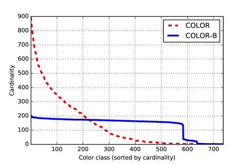
As our experiments show, the minimum number of colors for a valid coloring can be in the order of thousands in practice and hence, the number of subsets, $K$, cannot be set to a very small number. To solve this problem, for Color and Color-B, we have packed the color sets into $K$ bins such that each bin has almost an equal number of functions. Given $K$, the packing is performed in a greedy fashion by applying a first-fit policy and putting a color set into the first available bin having less than $|\mathcal{I}|/K$ functions. After the packing, the $k$th bin is used to form the subset $S_{k}$.

The second parallelization scheme we employed, Hogwild, does not consider synchronization at all (Recht et al., 2011). Hence, all the synchronization overhead can be avoided at the cost of computing a potentially inaccurate (partial) gradient. In this scheme, the functions in $\mathcal{I}$ are randomly distributed into $K$ subsets, where each subset $S_{k}$ for $k=1,\cdots,K$ contains (almost) the same number of functions. As in Color, a block is defined as a single-function. In this scheme, the parameter sets of the blocks in a subset can be overlapping, and when they are processed in parallel, some entries of the gradient may be computed incorrectly due to potential race conditions. Considering the large size of the parameter set in practice and the limit on the number of cores on a single machine, Hogwild assumes that there will be no error in the gradient, and even there is, its impact will be insignificant.

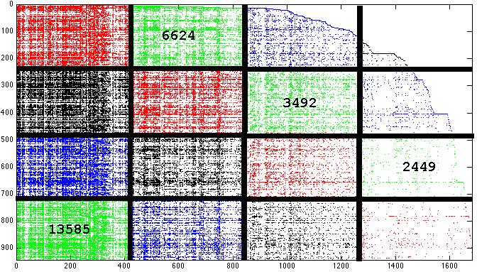
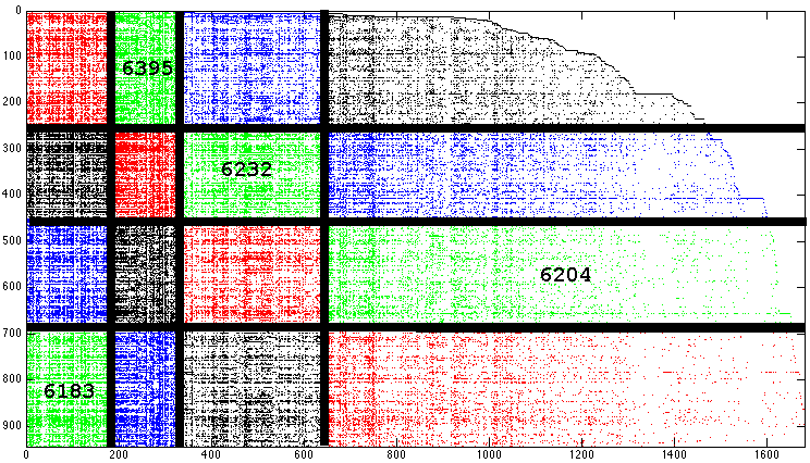
The third scheme we experimented is stratification that has previously been applied to parallelize stochastic gradient descent in a distributed-memory setting (Gemulla et al., 2011). When the functions and/or observations are in a structured, multi-dimensional form, such as a matrix or a tensor, stratification partitions the (parameter) dimensions into a number of intervals and form a number of function strata that are amenable to parallelization. Figure 5 shows two possible stratifications for the MovieLens 100K matrix that contains 100K ratings from 943 users (rows) on 1682 movies (columns). The functions in different strata are colored with different colors: each stratum in the figure corresponds to a subset $S_{k}$ for $k\in\{1,2,3,4\}$ and each small, colored rectangle corresponds to a block; i.e., $B_{k}=4$ for $k\in\{1,2,3,4\}$. Since the block intervals are different within each subset, the blocks of the same subset $S_{k}$ can be processed in parallel by $B_{k}$ threads. In the literature, equi-length intervals (formed by the long thick lines in the figure) have been used for stratification and we call this variant as Strata. The original scheme by Gemulla et al. (2011) does not consider the balance on the number of functions within the blocks of the same subset.

As Figure 5(a) shows, for Strata, the sparsity and irregularity of the datasets can yield an unbalanced function-to-block distribution, which implies a load imbalance for a parallel execution. For this reason, we propose a balanced stratification scheme, Strata-B, which aims to generate blocks that contain (almost) the same number of functions for each subset. For a single dimension, the intervals are generated as follows: Starting from an empty interval, the current interval is extended by one as long as it contains less than $|\mathcal{I}|/K$ functions. If the number of functions surpasses this value, the current interval is finalized and the next one is started. This process is repeated for each dimension to generate the blocks. This greedy procedure does not consider all the dimensions at once, and hence, it does not directly balance the number of functions within the rectangle block. However, according to our experiments, it performs much better than the original Strata scheme. For instance, for MovieLens 100K, the second block $S_{2}$ of a 4-way Strata contains blocks with 6624, 3492, 2449, and 13585 functions. As Figure 5(b) shows, these values for Strata-B are 6395, 6232, 6204 and 6183, respectively.

(a) Strata

(b) Strata-B

Figure 5. Two stratifications for the MovieLens 100K matrix that contains 100K ratings from 943 users (rows) on 1682 movies (columns). (Left) Strata uses equi-length intervals as suggested in the literature. (Right) Strata-B uses a greedy balancing heuristic with non-equal intervals. The numbers on the rectangles show the number of non-zeros/functions within that block.

1 input : $x$, schedule, $\eta$, $\gamma$ and ${\boldsymbol{\alpha}}_{k,b}$ for all $k=1,\cdots,K$; $b=1,\cdots,B_{k}$.

2 $t=1$, $S=\mathbf{0}$, $Y=\mathbf{0}$

3 ${\mathcal{K}}=[K,1,2,\cdots,K-1,K]$

4 repeat

5       $\beta_{t}=(\eta t)^{\gamma}$

6       $\mathcal{K}\leftarrow$ SetSchedule($\mathcal{K}$, schedule)

7       for $\ell=1,2,\cdots,K+1$ do

8             $k={\mathcal{K}}[\ell]$

9             for $b=1,2,\cdots,B_{k}$ do in parallel

10                   $g_{{\boldsymbol{\alpha}}_{k,b}}=\nabla f_{k,b}(x_{{\boldsymbol{\alpha}}_{k,b}})$

11                   if $\ell=1$ then

12                         $\bar{g}_{{\boldsymbol{\alpha}}_{k,b}}=g_{{\boldsymbol{\alpha}}_{k,b}}$, $\bar{x}_{{\boldsymbol{\alpha}}_{k,b}}=x_{{\boldsymbol{\alpha}}_{k,b}}$

13                        

14                  $x_{{\boldsymbol{\alpha}}_{k,b}}=x_{{\boldsymbol{\alpha}}_{k,b}}-\frac{1}{\beta_{t}}(\sigma g_{{\boldsymbol{\alpha}}_{k,b}}+W_{{\boldsymbol{\alpha}}_{k,b}}NW_{{\boldsymbol{\alpha}}_{k,b}}^{\top}g_{{\boldsymbol{\alpha}}_{k,b}})$

15                  

16            

17      $s=x-\bar{x}$, $y=g-\bar{g}$,

18       if $s^{\top}y>0$ then

19             $\sigma=\frac{s^{\top}y}{y^{\top}y}$

20             $S=[S(:,2:M),s]$,  $Y=[Y(:,2:M),y]$,  $W=[S,\ \sigma Y]$

21             $C=Y^{\top}Y$,  $R=\mbox{triu}(S^{\top}Y)$,  $D=\mbox{diag}(R)I$

22             $N=\left[\begin{array}[]{cc}R^{-\top}(D+\sigma C)R^{-1}&-R^{-\top}\\ -R^{-1}&0\end{array}\right]$

23            

24      $t\leftarrow t+1$

25      

26until convergence or $t$ > max_epochs

Algorithm 2 HAMSI with L-BFGS Updates

4. Example Implementation

We give a particular implementation of HAMSI in Algorithm 2 for illustrative purposes. Here, the approximate Hessian matrices are obtained using the BFGS quasi-Newton update formula. In particular, the compact form of limited memory BFGS (L-BFGS) is used in inner iterations to form the quadratic models and obtain their analytical solutions (Byrd et al., 1994). L-BFGS allows the computation of $(H^{(t)}+\beta_{t}I)^{-1}v$ for a given vector $v$ without forming any $|\mathcal{J}|\times|\mathcal{J}|$ matrices, and without any $\mathcal{O}(|\mathcal{J}|^{2})$ operations. Moreover, the memory requirement is only $\mathcal{O}(M|\mathcal{J}|)$, where $M$ is the memory size. This step corresponds to the exact solution of our subproblem in HAMSI (line 1 of Algorithm 1).

Quasi-Newton approximations require the difference of two consecutive iterates as well as the difference of the gradients evaluated at those iterates. In line 2 of Algorithm 2, we store the previous iterate as well as its gradient. Then, in line 2 the desired differences $s$ and $y$ are evaluated after the new iterate, $x$ and its gradient, $g$ are evaluated. A limited memory quasi-Newton algorithm uses a collection of $M$ such differences to update the approximate Hessian; we denote the corresponding memory matrices of size $|\mathcal{J}|\times M$ as $S$ and $Y$. The vector and matrix algebra operations from line 2 to line 2 are nothing else but the direct use of compact form formulas; we refer to (Byrd et al., 1994) for details.

In Algorithm 1, the SetSchedule function rotates over all the subsets in the same cyclic order. However, in the literature, it is also quite common to select the subsets randomly without replacement; cf. (Gemulla et al., 2011) In the next section, we shall compare our results against the random order. Therefore, in our example implementation we have also added one more parameter to the SetSchedule function. The parameter schedule can be either deterministic (det) or stochastic (stoc). The deterministic order is the one cyclic left-shift as in Algorithm 1. The stochastic order, on the other hand, obtains a temporary array by a random permutation of the first $K$ elements of $\mathcal{K}$ and then, appends this temporary array with the first element in the array. The resulting array then becomes the new $\mathcal{K}$ in line 1. An illustrative execution of the new SetSchedule function for $K=4$ is as follows:

Iteration	Deterministic	Stochastic
$t$	$\mathcal{K}=[3,4,1,2,3]$	$\mathcal{K}=[3,1,4,2,3]$
$t+1$	$\mathcal{K}=[4,1,2,3,4]$	$\mathcal{K}=[2,4,3,1,2]$
$t+2$	$\mathcal{K}=[1,2,3,4,1]$	$\mathcal{K}=[3,2,1,4,3]$
$\vdots$	$\vdots$	$\vdots$

All the vector and matrix operations (including the memory copy operations) in Algorithm 1 are parallelized; as stated, the gradient is computed in parallel by using the techniques in Section 3. For practical purposes, while processing the blocks of a subset $S_{k}$, we postpone the partial iterate updates at line 2 and do a single lazy update $x=x-\frac{1}{\beta_{t}}(\sigma g+WNW^{\top}g)$ once for each iteration of the for loop at line 2. Furthermore, for memory and cost efficiency, this update is performed (in parallel) from right-to-left; i.e., following the order in $W(N(W^{\top}g))$. In this way, we do not need to store $WNW^{\top}$ and perform three matrix-vector multiplications instead of expensive matrix-matrix multiplications. These operations are parallelized by block-partitioning of the columns and the rows of $W^{\top}$ and $W$, respectively. In addition, the (potentially expensive) shift operations for the matrices $S$ and $Y$ (at line 2) are avoided by inserting the new $s$ and $y$ vectors on top of an existing column in a round-robin fashion and only updating the corresponding row/column of $R=\mbox{triu}(S^{\top}Y)$ at every outer iteration.

5. Computational Study

All the simulation experiments in this section are performed on a single machine running on 64 bit CentOS 6.5 equipped with 384GB RAM and a dual-socket Intel Xeon E7-4870 v2 clocked at 2.30 GHz, where each socket has 15 cores (30 in total). Each core has a 32kB L1 and a 256kB L2 cache, and each socket has a 30MB L3 cache. All the codes are compiled with gcc 4.9.2 with the -O3 optimization flag enabled. For parallelization, we used OpenMP and for matrix operations, we use GSL v1.13 and compile the codes with options -lgsl -lgslcblas.

			Average Final RMSE Value
Dataset	Algorithm	schedule	Hogwild	Color	Color-B	Strata	Strata-B
$\underset{\text{ratings}}{1M}$ – $\underset{\text{users}}{6040}$- – $\underset{\text{movies}}{3883}$	mb-GD	det	3.1074	3.1061	3.0845	2.5315	2.4588
		stoc	3.1433	3.1470	3.1003	2.5325	2.4650
(25 seconds)	HAMSI	det	0.6901	0.6955	0.7102	0.6133	0.6022
		stoc	0.6900	0.7987	0.8017	0.6088	0.5994
$\underset{\text{ratings}}{10M}$ – $\underset{\text{users}}{71567}$ – $\underset{\text{movies}}{10681}$	mb-GD	det	4.3167	4.2676	4.2617	4.0029	3.4088
		stoc	4.3009	4.2863	4.2801	4.0035	3.4094
(250 seconds)	HAMSI	det	0.9279	1.0181	0.8941	0.8923	0.8643
		stoc	0.9207	1.1357	1.1229	0.8988	0.8652
$\underset{\text{ratings}}{20M}$ – $\underset{\text{users}}{138493}$ – $\underset{\text{movies}}{26744}$	mb-GD	det	4.8655	4.8051	4.8000	4.8093	3.8890
		stoc	4.8641	4.8279	4.8142	4.8091	3.8975
(500 seconds)	HAMSI	det	1.0170	1.1117	0.9521	1.0113	0.9042
		stoc	1.0112	1.2944	1.2220	1.0231	0.9035

Table 1. Root-mean square errors of all parallel execution strategies for mini-batch GD and HAMSI for three datasets. For each configuration, both algorithms are given the same initial solution, run for 25, 250, and 500 seconds on 1M, 10M and 20M rating datasets, respectively, with 16 threads. This experiment is performed three times with three different initial solutions and the average is reported.

5.1. Setup

For the experiments, we use the MovieLens datasets with 1M, 10M, and 20M ratings (Harper and Konstan, 2015). The number of entities (users and movies) for each dataset are given in Table 1. For each dataset, we form the corresponding User $\times$ Movie matrix and compute a factorization of rank $50$; i.e., the latent (inner) dimension of the factors is set to $50$. To compare the performance of HAMSI, we implemented the mini-batch gradient descent (mb-GD) as a baseline. In particular, both HAMSI and mb-GD use the same code base with minor differences: mb-GD uses a different schedule order $\mathcal{K}$ of size $K$ (instead of $K+1$), which is simply a permutation of $\{1,2,\cdots,K\}$ and the stochastic gradient update equation $x\leftarrow x-\frac{1}{\beta_{t}}g$ instead of the one altered with the approximate Hessian (line 2). We note that in the first few iterations, until full $S$ and $Y$ matrices are obtained, HAMSI also employs the gradient descent update. Clearly, mb-GD implementation does not perform any of the matrix operations at lines 2–2. The constant algorithm parameters are set as follows: for mb-GD, $(\eta=0.001,\gamma=0.51)$; for HAMSI, $(\eta=0.06,\gamma=0.51)$.

We carried out two sets of experiments: (I) fixed wallclock time and (II) fixed number of iterations. In the first set (I), we allocate a fixed optimization time for each algorithm and let the code run for $25$, $250$ and $500$ seconds for the datasets 1M, 10M and 20M, respectively. We report the training error, where we measure the quality of the final solution by the root-mean-square error (RMSE). We employed all 5 parallelization schemes, Hogwild, Color, Color-B, Strata, and Strata-B with $1,2,4,8$ and $16$ threads, and repeated each experiment three times with different random seeds used to generate the initial solutions. Overall, 3 (datasets) $\times$ 2 (algorithms) $\times$ 5 (parallelization scheme) $\times$ 5 ($\#$threads) $\times$ 3 (random seeds) $\times$ 2 (scheduling) $=900$ experiments are performed. For this set of experiments, the schemes Hogwild, Color and Color-B uses $K=20$ where Strata and Strata-B automatically sets $K$ to number of threads. As explained in Section 3, for Color and Color-B, we packed the color sets into $K=20$ large batches, since there were around $3500$, $35000$, and $65000$ color sets for the datasets 1M, 10M, and 20M respectively.

Table 1 shows the RMSE averages for parallel executions with 16 threads for the first experiment set (I). Since the algorithms are executed for a fixed amount of time but not for a fixed number of iterations, the parallelization scheme has a significant impact on the overall optimization performance. For both of the algorithms, Strata-B with a deterministic schedule is the best candidate in almost all the experiments. Furthermore, for HAMSI, the parallelization scheme Color-B is clearly better than Color. In general, HAMSI outperforms mini-batch GD in terms of the final RMSE value. Since both HAMSI and mb-GD use the same codebase, and mb-GD is allowed to perform more iterations in a fixed amount of time, we conclude that it pays well off doing the extra computations for the Hessian approximations overhead in HAMSI.

To compare the algorithms further, we select the best performing parameter settings from Table 1; that is, Strata-B scheme with deterministic scheduling. Figure 6 shows the progress of these mb-GD and HAMSI variants in terms of RMSE values. Clearly, HAMSI drastically improves the RMSE value for the corresponding problem much earlier than mb-GD. Furthermore, the differences in the attained RMSE values seem to increase with the size of the problem. This result also illustrates the performance gain obtained by using the second order information.

Figure 6. Convergence of mb-GD and HAMSI in terms RMSE values with 16 threads.

Our next discussion is about the changes in the convergence behavior of HAMSI when the number of threads is altered. Strata-B is used with a $K$ that is equal to the number of threads. Thus, the batch size becomes smaller when the number of threads increases. Consequently, the estimate of the original gradient deteriorates during the incremental steps leading to a somewhat high variance. However, Figure 7 shows that the performance of HAMSI is not affected significantly by the high variance gradient estimator. On the contrary, HAMSI seems to converge quickly for all problems when the number of threads is increased. This point is complementary to our observations in the next subsection, where we have demonstrated that HAMSI scales nicely with more computational resources.

Figure 7. Convergence behaviors of HAMSI when the number of threads is increased.

5.2. Efficiency of Parallelization

To further analyze the efficiency of the parallelization schemes and understand the differences in the final RMSE values, we partition the cost of an outer iteration into three phases: (i) data pass and gradient computation (line 2 of Algorithm 2); (ii) performing the updates (line 2 of Algorithm 2); (iii) maintaining the approximate Hessian (lines 2–2 of Algorithm 2).

(a) 1M

(b) 10M

(c) 20M

Figure 8. Hessian computation, update, and gradient computation time for an outer iteration of mb-GD and HAMSI with 16 threads.

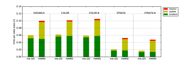
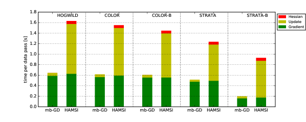
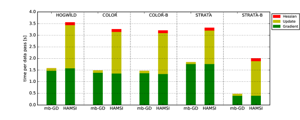
Figure 8 shows the times spent for these three phases with 16 threads. With HAMSI, the Hessian approximation is much cheaper than the other two phases. With mb-GD, computing the gradient, not surprisingly, is the main bottleneck. Hence, the parallelization schemes proposed in this work can be used to make a gradient-descent-based algorithm faster, and hence, more effective in practice. As mentioned above, although mb-GD performs $2$-$4\times$ more iterations per experiment, as Table 1 and Figure 6 show, HAMSI’s final RMSE values are much better than that of mb-GD’s.

Among all the parallelization schemes, Strata-B is the best one in terms of computational efficiency. Indeed, Strata-B is expected to be better than Strata, since the load is distributed to the threads more evenly. In addition, with Strata-B, each thread accesses a specific/narrowed part of $x$ and $g$. However, with Hogwild and coloring based schemes, the $x$ and $g$ locations accessed by a single thread, are distributed among all $x$ and $g$. Hence, stratification is expected to be a more cache-friendly parallelization scheme. To verify this, we performed a second set of experiments with 16 threads for which, each HAMSI variant, which employs a different parallelization scheme, is run for $100$ (outer) iterations and the cache miss ratios are observed with the perf command. To perform the same number of gradient computations, we keep $K=16$ for all the parallelization schemes in this experiment. Furthermore, by taking the function-to-thread assignment into account for each scheme and assuming that each function takes a unit time to process, we computed the total parallel gradient computation work for an outer iteration which is equal to

$$parWork=\sum_{k=1}^{K}{\lceil|S_{k}|/16\rceil}\mbox{\ \ \ \ and\ \ \ \ }parWork=\sum_{k=1}^{K}{\max_{b\in\{1,\cdots,B_{k}\}}\left(|S_{k,b}|\right)}.$$

The former one is for Hogwild, Color and Color-B, and the latter one is for Strata and Strata-B. The experiments are performed three times with three different initial solutions. Table 2 shows the averages of these experiments.

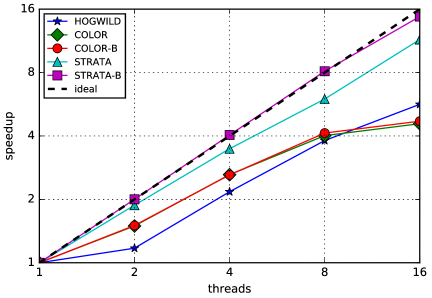
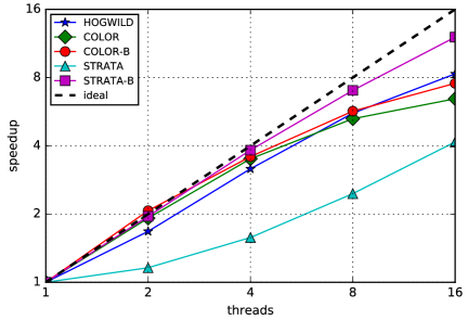
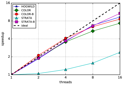
As expected, although Hogwild perfectly balances the load, it has the worst cache-miss ratio average. Furthermore, the stratification-based schemes are more cache friendly compared to others. Among them, Strata suffers due to a high $parWork$ value especially for $10M$ and $20M$ rating datasets and it is one of the slowest. On the other hand, Strata-B is the fastest, since it also solves the load balancing problem thanks to the proposed greedy approach to create balanced blocks. The performance difference between Strata-B and Hogwild (as well as Color and Color-B) is significant since the cost of a cache access increase $3$ to $4$ times for each cache level. Moreover, the impact of being cache friendly will be more important with increasing number of threads and larger datasets. Figure 9 shows the speedups for the gradient computation phase of HAMSI for all the datasets: Strata-B, as expected, is more scalable than the other schemes investigated in this work.

There exist other studies in the literature that aims providing load imbalance and good cache utilization at the same time. For instance, recently Pan et al. (2016) proposed Cyclades that samples and uses small, connected subgraphs of the function graph. They compared the performance of the proposed method with that of Hogwild on SGD with the 10M rating dataset. Connectivity implies cache locality up to some extent; indeed, a set of connected functions touch common factors. However, the corresponding subgraph of the factor graph may not be well-connected, where the connectedness, which is correlated with data reuse, can be quantified with clustering coefficients, edge-to-vertex ratio, etc. Furthermore, without arranging the locations of the factors on memory, e.g., via relabeling and modifying the input in a preprocessing phase, it is not possible to exploit the full potential of the connectivity. For instance, Pan et al. reported that with 16 threads, their partitioining phase takes as much time as 5.5 full data passes, i.e., outer iterations, of Hogwild where a single Hogwild data pass takes 0.48 seconds; with Cyclades the runtime reduces to 0.42 seconds. Although HAMSI is a second-order incremental algorithm and hence not exactly comparable with Cyclades, looking to mb-GD (which is also not directly comparable but the closest one we have), a full data pass takes 0.63 seconds for Hogwild on 10M rating dataset. Note that Cyclades experiments are performed on an 18-core Intel Xeon E7-8870 v3 with 576kB L1, 4.5MB L2, and 45MB L3 caches (32kB, 256kB, and 30MB, respectively, for our processor). Hence, due to possible implementation differences and a significantly better cache hierarchy, the runtime for Hogwild is better. However, the Strata-B parallelization of mb-GD reports 0.2 seconds for a full data pass on the same dataset which is 3$\times$ better than Hogwild where the improvement is around $15\%$ for Cyclades. This is expected since Strata-B respects the initial data labels, and hence, how the factor data is organized in the memory. Furthermore, since it only employs a cheap load-balancing heuristic, Strata-B’s preprocessing phase, performed only once, is 50$\times$ faster than a single data pass of Hogwild.

1M
Scheme	L1-dL ($\times 10^{9}$)	L1-m ($\%$)	L2-m ($\%$)	L3-m ($\%$)	$parWork$	RMSE	Time (sec)
Hogwild	75.0	13.1	8.7	1.7	62513	0.82	8.7
Color	74.8	11.8	5.5	1.1	64354	0.82	8.4
Color-B	75.0	11.9	5.6	1.2	64193	0.82	8.6
Strata	74.5	8.8	2.3	0.4	98087	0.83	4.8
Strata-B	74.3	8.8	2.3	0.4	69145	0.82	4.3
10M
Scheme	L1-dL ($\times 10^{9}$)	L1-m ($\%$)	L2-m ($\%$)	L3-m ($\%$)	$parWork$	RMSE	Time (sec)
Hogwild	666.7	13.2	10.2	3.0	625003	1.03	136.5
Color	673.6	11.8	7.6	1.6	642486	1.20	124.9
Color-B	672.6	11.9	7.7	1.7	641484	0.97	122.1
Strata	673.0	8.8	3.9	0.9	2535881	1.03	128.9
Strata-B	672.0	8.6	3.7	0.9	659763	1.01	95.1
20M
Scheme	L1-dL ($\times 10^{9}$)	L1-m ($\%$)	L2-m ($\%$)	L3-m ($\%$)	$parWork$	RMSE	Time (sec)
Hogwild	1328.5	13.3	10.5	3.9	1250016	1.12	304.6
Color	1354.9	11.7	7.9	2.1	1284808	1.28	269.8
Color-B	1381.2	11.7	8.0	2.2	1281179	1.05	270.3
Strata	1331.8	9.0	5.0	1.1	8726743	1.13	326.8
Strata-B	1331.7	8.8	4.2	1.1	1289630	1.12	189.1

Table 2. Cache miss ratios, $parWork$ and RMSE values, and the execution times of HAMSI variants when different parallelization schemes are employed with $K=16$ and 16 threads for the datasets with 1M, 10M and 20M ratings. The first column is the number of L1-cache data load requests performed by the execution, and the next three columns are percentages with respect to the first column.

(a) 1M

(b) 10M

(c) 20M

Figure 9. Speedups obtained on the gradient computation phase for each parallelization scheme with $1$, $2$, $4$, $8$ and $16$ threads for 1M, 10M, and 20M rating datasets.

6. Conclusion and Future Work

In this work, we propose HAMSI, Hessian Approximated Multiple Subsets Iteration, a provably convergent incremental algorithm for solving large-scale partially separable optimization problems that frequently emerge in machine learning and demonstrate its use in a matrix factorization problem with missing values. HAMSI may be considered as a viable alternative in many scenarios in practice as we empirically show in our matrix-factorization experiments. In the near future, we are planning to adopt the proposed optimization techniques as well as the parallelization schemes to other problems such as logistic regression, neural network training and tensor factorization.

HAMSI currently solves unconstrained optimization problems. However, in several applications, like nonnegative matrix factorization, there could be simple constraints that need to be taken into account. Although one can devise a straightforward projection step to maintain feasibility, our current analysis does not guarantee convergence. Incorporating simple constraints is in our future research agenda.

An interesting observation from Table 2 is that with fixed number of iterations, Color is the worst scheme in terms of RMSE values while Color-B is the best one. What differs these schemes from the others is an implicit high coverage of the gradient entries for each subset. Indeed, a valid coloring puts independent functions to the same set. Hence these functions will cover different gradient locations. However, the traditional first-fit policy employed by Color generates a few massive color sets with a (probably) full coverage and many small color sets covering only a few positions. Since the gradient descent variants perform the updates by following only these touched positions, the optimization process may be deteriorated with the restricted moves implied by Color. However, with Color-B, the problem will mostly be solved. We claim that although Color-B does not improve the computational efficiency due to a limited number of cores on a shared-memory machine, with a fixed number of iterations, its RMSE value is lower compared to other schemes since its gradient coverage is much better. Although we believe that this is an interesting claim needs to be proven, the investigation of such a claim is beyond the motivation of this study. In the future, we will analyze the impact of coverage on the optimization efficiency and investigate various parallelism schemes featuring a better gradient coverage, load balance, and cache locality at the same time.

Appendix A Omitted Proofs

Proof of Lemma 2.1

By using Assumption A.2, we have

$$\begin{array}[]{rl}\|\nabla f_{S_{[l]}}(x^{(t,l-1)})-\nabla f_{S_{[l]}}(x^{(t)})\|&\leq L\|x^{(t,l-1)}-x^{(t)}\|\\[5.69054pt] &=L\|x^{(t,l-1)}-x^{(t,l-2)}+x^{(t,l-2)}-x^{(t,l-3)}+\cdots+x^{(t,1)}-x^{(t)}\|\\[5.69054pt] &\leq L\sum_{j=1}^{\ell-1}\|x^{(t,j)}-x^{(t,j-1)}\|.\end{array}$$

Note for $j=1,\cdots,\ell-1$ that

$$\|x^{(t,j)}-x^{(t,j-1)}\|=\|x^{(t,j-1)}-(H^{(t)}+\beta_{t}I)^{-1}\nabla f_{S_{[j]}}(x^{(t,j-1)})-x^{(t,j-1)}\|\leq M_{t}C,$$

where the last inequality holds by Assumption A.4. Therefore, we have

$$\|\nabla f_{S_{[l]}}(x^{(t,l-1)})-\nabla f_{S_{[l]}}(x^{(t)})\|\leq LM_{t}C(\ell-1).$$

Proof of Lemma 2.2

At iteration $t+1$, we have

$$\begin{array}[]{rl}x^{(t+1)}&=x^{(t)}-\sum_{\ell=1}^{K+1}(H^{(t)}+\beta_{t}I)^{-1}\nabla f_{S_{[\ell]}}(x^{(t,\ell-1)})\\[5.69054pt] &=x^{(t)}-(H^{(t)}+\beta_{t}I)^{-1}\nabla f(x^{(t)})\\[5.69054pt] &\hskip 14.22636pt+(H^{(t)}+\beta_{t}I)^{-1}\sum_{\ell=1}^{K+1}(\nabla f_{S_{[\ell]}}(x^{(t)})-\nabla f_{S_{[\ell]}}(x^{(t,\ell-1)})).\end{array}$$

This shows that

(12) $$x^{(t+1)}-x^{(t)}=\Delta_{t}-(H^{(t)}+\beta_{t}I)^{-1}\nabla f(x^{(t)}),$$

where

$$\Delta_{t}\equiv(H^{(t)}+\beta_{t}I)^{-1}\sum_{\ell=1}^{K+1}(\nabla f_{S_{[\ell]}}(x^{(t)})-\nabla f_{S_{[\ell]}}(x^{(t,\ell-1)})).$$

Using now (10) implies

(13) $$\begin{array}[]{rl}\|\Delta_{t}\|&\leq M_{t}\sum_{\ell=1}^{K+1}\|\nabla f_{S_{[\ell]}}(x^{(t)})-\nabla f_{S_{[\ell]}}(x^{(t,\ell-1)})\|\\[5.69054pt] &\leq M_{t}\sum_{\ell=1}^{K+1}LM_{t}C(\ell-1)=\frac{1}{2}LM^{2}_{t}CK(K+1)=BM_{t}^{2}.\\[5.69054pt] \end{array}$$

Then, we obtain

$$\begin{array}[]{rl}\|x^{(t+1)}-x^{(t)}\|&=\|\Delta_{t}-(H^{(t)}+\beta_{t}I)^{-1}\nabla f(x^{(t)})\|\\[5.69054pt] &\leq\|\Delta_{t}\|+\|(H^{(t)}+\beta_{t}I)^{-1}\|\nabla f(x^{(t)})\|\\[5.69054pt] &\leq BM_{t}^{2}+CM_{t}\leq\frac{B+C(M+1)}{M+1}M_{t}.\end{array}$$

Proof of Theorem 2.3

As $f$ is a twice differentiable function, we have

$$f(x^{(t+1)})-f(x^{(t)})\leq{\nabla f(x^{(t)})}^{T}(x^{(t+1)}-x^{(t)})+\frac{LK}{2}\|x^{(t+1)}-x^{(t)}\|^{2}.$$

Using now Lemma 2.2 along with (12) and (13), we obtain

(14) $$\begin{array}[]{rl}f(x^{(t+1)})-f(x^{(t)})&\leq\nabla f(x^{(t)})^{T}\Delta_{t}-\nabla f(x^{(t)})^{T}(H^{(t)}+\beta_{t}I)^{-1}\nabla f(x^{(t)})+\frac{LK}{2}\|x^{(t+1)}-x^{(t)}\|^{2}\\[5.69054pt] &\leq\|\nabla f(x^{(t)})\|\||\Delta_{t}\|-U_{t}\|\nabla f(x^{(t)})\|^{2}+\frac{LK}{2}\left(\frac{B+C(M+1)}{M+1}\right)^{2}M^{2}_{t}\\[5.69054pt] &\leq-U_{t}\|\nabla f(x^{(t)})\|^{2}+\bar{B}M^{2}_{t},\end{array}$$

where $\bar{B}\equiv CB+\frac{LK}{2}\left(\frac{B+C(M+1)}{M+1}\right)^{2}$. Due to Assumption A.1, we can write $\inf_{x\in\mathbb{R}^{n}}f(x)=f^{*}>-\infty$. Thus, we obtain

$$0\leq f(x^{(t+1)})-f^{*}\leq f(x^{(t)})-f^{*}+\bar{B}M^{2}_{t}.$$

Relation (11) and Lemma 2.2 in (Mangasarian and Solodov, 1994) together show that the sequence $\{f(x^{(t)})\}$ converges. By using (14), we further have

$$\begin{array}[]{rl}f(x^{(1)})-f^{*}&\geq f(x^{(1)})-f(x^{(t)})=\sum_{j=1}^{t-1}(f(x^{(t)})-f(x^{(t+1)}))\\[5.69054pt] &\geq\sum_{j=1}^{t-1}U_{j}\|\nabla f(x^{(j)})\|^{2}-\bar{B}\sum_{j=1}^{t-1}M^{2}_{j}\\[5.69054pt] &\geq\underset{1\leq j\leq t-1}{\inf}\|\nabla f(x^{(j)})\|^{2}\sum_{j=1}^{t-1}U_{j}-\bar{B}\sum_{j=1}^{t-1}M^{2}_{j}.\end{array}$$

Let now $t\rightarrow\infty$, then

(15) $$f(x^{(1)})-f^{*}\geq\inf_{j\geq 1}\|\nabla f(x^{(j)})\|^{2}\sum_{j=1}^{\infty}U_{j}-\bar{B}\sum_{j=1}^{\infty}M^{2}_{j}.$$

Using again Assumption A.1 and conditon (11), we obtain

(16) $$\inf_{t\geq 1}\|\nabla f(x^{(t)})\|=0.$$

Now, suppose for contradiction that the sequence $\{\nabla f(x^{(t)})\}$ does not converge to zero. Then, there exists an increasing sequence of integers such that for some $\varepsilon>0$, we have $\|\nabla f(x^{(t_{\tau})})\|\geq\varepsilon$ for all $\tau$. On the other hand, the relation (16) implies that there exist some $j>t_{\tau}$ such that $\|\nabla f(x^{(j)})\|\leq\frac{\varepsilon}{2}$. Let $j_{\tau}$ be the least integer for each $\tau$ satisfying these inequalities. Then, we have

$$\begin{array}[]{rl}\frac{\varepsilon}{2}&\leq\|\nabla f(x^{(t_{\tau})})\|-\|\nabla f(x^{(j_{\tau})})\|\\[5.69054pt] &\leq\|\nabla f(x^{(t_{\tau})})-\nabla f(x^{(j_{\tau})})\|\\[5.69054pt] &\leq LK\|x^{(t_{\tau})}-x^{(j_{\tau})}\|\leq LK\frac{B+C(M+1)}{M+1}\sum_{k=t_{\tau}}^{j_{\tau}-1}M_{k},\end{array}$$

where the last inequality follows from Lemma 2.2. Since $0<M\leq U$, there exists $\zeta\leq\frac{M}{U}\leq 1$ such that

$$M+\beta_{k}\geq\zeta U+\beta_{k}\geq\zeta(U+\beta_{k})\implies M_{k}\leq\frac{1}{\zeta}U_{k}.$$

Thus, we obtain

$$0<\hat{B}\equiv\frac{\varepsilon(M+1)\zeta}{2LK(B+C(M+1))}\leq\sum_{k=t_{\tau}}^{j_{\tau}-1}U_{k}.$$

Then, using together with inequality (14), we obtain

$$\begin{array}[]{rl}f(x^{(t_{\tau})})-f(x^{(j_{\tau})})&\geq\sum_{k=t_{\tau}}^{j_{\tau}-1}U_{k}\|\nabla f(x^{(k)})\|^{2}-\bar{B}\sum_{k=t_{\tau}}^{j_{\tau}-1}M_{k}^{2}\\[5.69054pt] &\geq\hat{B}\underset{t_{\tau}\leq k\leq j_{\tau}-1}{\inf}\|\nabla f(x^{(k)})\|^{2}-\bar{B}\sum_{k=t_{\tau}}^{\infty}M_{k}^{2}.\end{array}$$

Since the left-hand-side of the inequality converges and the condition (11) holds, we have

(17) $$\lim_{\tau\uparrow\infty}\leavevmode\nobreak\ \underset{t_{\tau}\leq k\leq j_{\tau}-1}{\inf}\|\nabla f(x^{(k)})\|^{2}=0.$$

But our choice of $t_{\tau}$ and $j_{\tau}$ guarantees $\|\nabla f(x^{(k)})\|>\frac{\varepsilon}{2}$ for all $t_{\tau}\leq k\leq j_{\tau}$, and hence, we arrive at a contradiction with (17). Therefore, ${\nabla f(x^{(t)})}$ converges, and with the continuity of the gradient, we conclude for each accumulation point $x^{*}$ of the sequence $\{x^{(t)}\}$ that $\nabla f(x^{*})=0$ holds.

References

- (1)
- Berahas et al. (2016) A.S. Berahas, J. Nocedal, and M. Takáč. 2016. A Multi-Batch L-BFGS Method for Machine Learning. (2016), 1055–1063. http://papers.nips.cc/paper/6145-a-multi-batch-l-bfgs-method-for-machine-learning
- Bertsekas (1996) D.P. Bertsekas. 1996. Incremental least squares methods and the extended Kalman filter. SIAM Journal on Optimization 6, 3 (1996), 807–822.
- Bertsekas (2011) D.P. Bertsekas. 2011. Incremental gradient, subgradient, and proximal methods for convex optimization: A survey. Optimization for Machine Learning 2010 (2011), 1–38.
- Blatt et al. (2007) D. Blatt, A.O. Hero, and H. Gauchman. 2007. A convergent incremental gradient method with a constant step size. SIAM Journal on Optimization 18, 1 (2007), 29–51.
- Bozdağ et al. (2010) D. Bozdağ, Ü.V. Çatalyürek, A.H. Gebremedhin, F. Manne, E.G. Boman, and F. Özgüner. 2010. Distributed-memory Parallel Algorithms for Distance-2 Coloring and Related Problems in Derivative Computation. SIAM Journal on Scientific Computing 32, 4 (2010), 2418–2446. DOI:http://dx.doi.org/10.1137/080732158
- Byrd et al. (1994) R.H. Byrd, J. Nocedal, and R.B. Schnabel. 1994. Representations of quasi-Newton matrices and their use in limited memory methods. Mathematical Programming 63, 1-3 (1994), 129–156.
- Byrd et al. (2016) R. H. Byrd, S.L. Hansen, J. Nocedal, and Y. Singer. 2016. A Stochastic Quasi-Newton Method for Large-Scale Optimization. SIAM Journal on Optimization 26, 2 (2016), 1008–1031. DOI:http://dx.doi.org/10.1137/140954362
- Cichocki et al. (2009) A. Cichocki, R. Zdunek, A. H. Phan, and S. Amari. 2009. Nonnegative Matrix and Tensor Factorization. Wiley.
- Gebremedhin et al. (2002) A.H. Gebremedhin, F. Manne, and A. Pothen. 2002. Parallel distance-k coloring algorithms for numerical optimization. In Euro-Par 2002 Parallel Processing - 8th International Conference. 912–921.
- Gebremedhin et al. (2005) A.H. Gebremedhin, F. Manne, and A. Pothen. 2005. What Color is Your Jacobian? Graph Coloring for Computing Derivatives. SIAM Rev. 47, 4 (2005), 629–705.
- Gebremedhin et al. (2013) A.H. Gebremedhin, D. Nguyen, Md. M.A. Patwary, and A. Pothen. 2013. ColPack: Software for Graph Coloring and Related Problems in Scientific Computing. ACM Trans. Math. Softw. 40, 1, Article 1 (Oct. 2013), 31 pages.
- Gemulla et al. (2011) R. Gemulla, E. Nijkamp, P.J. Haas, and Y. Sismanis. 2011. Large-scale matrix factorization with distributed stochastic gradient descent. In ACM SIGKDD.
- Gower et al. (2016) R.M. Gower, D. Goldfarb, and P. Richtárik. 2016. Stochastic Block BFGS: Squeezing More Curvature out of Data. In Proceedings of The 33rd International Conference on Machine Learning (Proceedings of Machine Learning Research), Maria Florina Balcan and Kilian Q. Weinberger (Eds.), Vol. 48. PMLR, New York, New York, USA, 1869–1878. http://proceedings.mlr.press/v48/gower16.html
- Gürbüzbalaban et al. (2014) M. Gürbüzbalaban, A. Ozdaglar, and P. Parrilo. 2014. A globally convergent incremental Newton method. arXiv preprint arXiv:1410.5284 (2014).
- Harper and Konstan (2015) F.M. Harper and J.A. Konstan. 2015. The MovieLens Datasets: History and Context. ACM Trans. Interact. Intell. Syst. 5, 4, Article 19 (Dec. 2015), 19 pages. DOI:http://dx.doi.org/10.1145/2827872
- Kschischang et al. (2001) F.R. Kschischang, B.J. Frey, and H-A. Loeliger. 2001. Factor graphs and the sum-product algorithm. IEEE Transactions on Information Theory 47, 2 (2001), 498–519.
- Mangasarian and Solodov (1994) O.L. Mangasarian and M.V. Solodov. 1994. Serial and parallel backpropation convergence via nonmonotone perturbed minimization. Optimization Methods and Software 4 (1994), 103–116.
- Matula (1968) D. W. Matula. 1968. A min-max theorem for graphs with application to graph coloring. SIAM Rev. 10 (1968), 481–482.
- Moritz et al. (2015) P. Moritz, R. Nishihara, and M.I. Jordan. 2015. A Linearly-Convergent Stochastic L-BFGS Algorithm. arXiv preprint arXiv:1508.02087 (2015).
- Pan et al. (2016) X. Pan, M. Lam, S. Tu, D. Papailiopoulos, S. Zhang, M.I. Jordan, K. Ramchandran, and C. Ré. 2016. Cyclades: Conflict-free Asynchronous Machine Learning. In Advances in Neural Information Processing Systems 29, D. D. Lee, M. Sugiyama, U. V. Luxburg, I. Guyon, and R. Garnett (Eds.). Curran Associates, Inc., 2568–2576. http://papers.nips.cc/paper/6604-cyclades-conflict-free-asynchronous-machine-learning.pdf
- Recht et al. (2011) B. Recht, C. Re, S. Wright, and N. Feng. 2011. Hogwild: A Lock-Free Approach to Parallelizing Stochastic Gradient Descent. In Advances in Neural Information Processing Systems 24, J. Shawe-Taylor, R. S. Zemel, P. L. Bartlett, F. Pereira, and K. Q. Weinberger (Eds.). Curran Associates, Inc., 693–701. http://papers.nips.cc/paper/4390-hogwild-a-lock-free-approach-to-parallelizing-stochastic-gradient-descent.pdf
- Roux et al. (2012) N.L. Roux, M. Schmidt, and F.R. Bach. 2012. A stochastic gradient method with an exponential convergence _rate for finite training sets. In Advances in Neural Information Processing Systems. 2663–2671.
- Schraudolph et al. (2007) N.N. Schraudolph, J. Yu, and S. Gunter. 2007. A Stochastic Quasi-Newton Method for Online Convex Optimization. In Proceedings of the 11th International Conference Artificial Intelligence and Statistics (AISTATS). 433–440.
- Shamir et al. (2014) O. Shamir, N. Srebro, and T. Zhang. 2014. Communication Efficient Distributed Optimization using an Approximate Newton-type Method. In International Conference on Machine Learning (ICML).
- Singh and Gordon (2008) A. P. Singh and G. J. Gordon. 2008. A Unified View of Matrix Factorization Models. In European Conference on Machine Learning and Principles and Practice of Knowledge Discovery in Databases, Part II. Springer, 358–373.
- Sohl-Dickstein et al. (2014) J. Sohl-Dickstein, B. Poole, and S. Ganguli. 2014. Fast large-scale optimization by unifying stochastic gradient and quasi-Newton methods. In Proceedings of the 31th International Conference on Machine Learning (ICML). 604–612.
- Solodov (1998) M.V. Solodov. 1998. Incremental gradient algorithms with stepsizes bounded away from zero. Computational Optimization and Applications 11, 1 (1998), 23–35.
- Tseng (1998) P. Tseng. 1998. An incremental gradient (-projection) method with momentum term and adaptive stepsize rule. SIAM Journal on Optimization 8, 2 (1998), 506–531.
- Wang et al. (2014) X. Wang, S. Ma, and W. Liu. 2014. Stochastic Quasi-Newton Methods for Nonconvex Stochastic Optimization. arXiv preprint arXiv:1412.1196 (2014).
- Zuckerman (2007) D. Zuckerman. 2007. Linear Degree Extractors and the Inapproximability of Max Clique and Chromatic Number. Theory of Computing 3 (2007), 103–128.