Early-warning indicators for rate-induced tipping

Abstract

A dynamical system is said to undergo rate-induced tipping when it fails to track its quasi-equilibrium state due to an above-critical-rate change of system parameters. We study a prototypical model for rate-induced tipping, the saddle-node normal form subject to time-varying equilibrium drift and noise. We find that both most commonly used early-warning indicators, increase in variance and increase in autocorrelation, occur not when the equilibrium drift is fastest but with a delay. We explain this delay by demonstrating that the most likely trajectory for tipping also crosses the tipping threshold with a delay and therefore the tipping itself is delayed. We find solutions of the variational problem determining the most likely tipping path using numerical continuation techniques. The result is a systematic study of the most likely tipping time in the plane of two parameters, distance from tipping threshold and noise intensity.

The notion of tipping describes the phenomenon that at certain critical levels or rates the output of a system changes disproportionately compared to the change in input. Two particular examples in climate science are the possible collapse of the Atlantic Meridional Overturning Circulation (AMOC) due to increasing freshwater input or the sudden release of carbon in peatlands due to an external temperature increase above a critical rate (the compost bomb instability Wieczorek et al. (2011)). There is an ongoing debate, for example, in climate science Boulton, Allison, and Lenton (2014) and ecology Xu et al. (2015) whether it is possible to find early-warning indicators robustly in time series of system outputs before tipping occurs.

This paper focuses on the case of rate-induced tipping, which describes the scenario where a system fails to track its equilibrium due to a rapid change in parameters. We show that two popular candidates for early-warning indicators in time series, an increase in autocorrelation and an increase in variance, appear to give a delayed warning signal for tipping. We study the phenomenon by looking at the interaction of rate-induced tipping and noise. We find that the most likely time for the noise to kick the system over the threshold (which is a curve in phase space) is after the point where the threshold is closest to the equilibrium. We investigate this tipping (and, correspondingly, early-warning) delay systematically depending on two parameters: the distance of the parameter drift speed from its critical value and the noise intensity. We find that the delay is larger for smaller noise-intensity.

I Introduction

Tipping events are often described as sudden, disproportionate changes in output levels caused by small changes to input levels Ashwin, Perryman, and Wieczorek (2015). These can be irreversible events that have huge, unwanted consequences. Therefore, the study of early-warning indicators is of great interest and so recent research has developed and analyzed early-warning indicators, see Lenton (2011) for a review up to 2011 and Williamson and Lenton (2015) for references to later results. A few currently debated examples of complex systems deemed vulnerable to tipping from climate science, ecology and financial markets are: the abrupt reductions in Arctic summer sea ice Holland, Bitz, and Tremblay (2006), the collapse of the Atlantic Meridional Overturning Circulation (AMOC) Held and Kleinen (2004), the dieback of the Amazon rainforest Malhi et al. (2009), Australian ecosystemsLaurance et al. (2011), the light-driven regime shifts in polar ecosystems Clark et al. (2013), the collapse of coral reefs due to global warming and ocean acidification Hoegh-Guldberg et al. (2007), and crashes and rebounds of financial markets Yan, Woodard, and Sornette (2010). See also Lenton et al. (2008) for a list of policy-relevant tipping elements in the climate system. Ashwin et al. (2012) identified a few mathematical mechanisms behind the observed phenomena, attempting a classification:

• Bifurcation-induced tipping (Slow passage through a bifurcation)

• Noise-induced tipping (Transition between attractors due to random fluctuations)

• Rate-induced tipping (Failure to track a continuously changing quasi-steady state).

This paper studies how a system that is close to a rate-induced tipping event behaves under the influence of additive noise. We look at a prototypical system, the saddle-node normal form with additive noise and a ramped shift of the equilibrium as proposed by Ashwin et al. (2012). (A more general definition and further properties of rate-induced tipping are given by Ashwin, Perryman, and Wieczorek (2015).) Two early-warning indicators that are commonly used for bifurcation-induced tipping with noise are an increase of autocorrelation and an increase in variance in observed time series of system outputs Scheffer et al. (2009). The most common argument, why a generic output time series of a system approaching bifurcation-induced tipping should show an increase in autocorrelation and variance assumes that the bifurcation of the deterministic part is a saddle-node bifurcation. Far away from the bifurcation one can think of the state of the system as the position of an overdamped particle at the bottom of a slowly softening potential well. Any small perturbation or disturbance will relax back to the equilibrium with a large decay rate Scheffer et al. (2012). As the bifurcation is approached, the potential well will become shallower, that is, the decay rate will decrease Kuehn (2015). Thus, any disturbance or perturbation will have an increased and more long-lasting effect such that, in the presence of noise, autocorrelation and variance in observed time series increases.

In practice, the early-warning indicators are used on observational time series data of systems where quantitatively accurate models are unavailable, such as palaeoclimate temperature and CO₂ proxies Ditlevsen and Johnsen (2010) and lake eutrophication Wang et al. (2012). In the cited cases the early-warning indicators were not used for prediction (as they were about events in the past), but as evidence for (or against) the presence of underlying tipping mechanisms. For example, Dakos et al. (2008) used an increase in autocorrelation in a sequence of palaeoclimate time series as evidence for bifurcation-induced tipping while Ditlevsen and Johnsen (2010) used the absence of the increase in variance (and the inconclusive behavior of the autocorrelation) as evidence that the Dansgaard-Oeschger events are a case of noise-induced tipping. Similarly, the presence of early-warning indicators in simulation data from a global circulation model showing a collapse of the Atlantic Meridional Overturning circulation (AMOC) through freshwater input was used as evidence for a bifurcation-induced tipping event Boulton, Allison, and Lenton (2014). All of the cited studies base their arguments on the knowledge that, close to a bifurcation- or noise-induced tipping point the system (after de-trending) behaves like an Ornstein-Uhlenbeck (OU) process. For the OU process one can infer from observed autocorrelation and variance the underlying linear decay rate, thus, permitting conclusions about the approach (or lack of it) of the equilibrium to a saddle-node bifurcation. This paper studies the effect of noise on the third mechanism from the list by Ashwin et al. (2012), rate-induced tipping, with the goal to aid identification of this type from time series.

In contrast to bifurcation-induced tipping, rate-induced tipping is failure of the system to track the continuously changing quasi-steady state Ashwin et al. (2012). Unlike bifurcation-induced tipping, at each moment in time there exists a stable (quasi-)equilibrium but the rate at which this steady state shifts determines whether the system tips or not.

The effect of rate-induced tipping has been described only relatively recently. In particular, within climate science Wieczorek et al. (2011) considered a model for carbon storage and release in peatland soil, which showed the compost bomb instability. In their model an increase in temperature above a critical rate results in a release of carbon into the atmosphere from combustion of compost heaps. A higher CO₂ concentration in the atmosphere, creates further warming and thus triggering a positive feedback loop within the system Luke and Cox (2011). This is an example of rate-induced tipping as for every fixed atmospheric temperature there exists a globally stable steady state but the rapidity of the temperature increase causes sharp peaks of carbon release. Other examples of rate-induced tipping include the switching off of the AMOC due to the rate of increase of CO₂ in the atmosphere Stocker and Schmittner (1997). Scheffer et al. (2008) find in a plant-herbivore model the critical rates of plant growth causing a rate-induced transition from a herbivore controlled state to a vegetated state.

Rate-induced tipping is not associated to a loss of stability of equilibrium and thus cannot be explained using stability theory for equilibriaPerryman and Wieczorek (2014). An appropriate analogue to the“overdamped particle in a softening well” illustration for bifurcation-induced tipping is to think of an overdamped particle in a moving well. In contrast to bifurcation-induced tipping, the shape of the potential well remains constant but instead shifts at varying rates. The faster the shift the further the particle drifts away from the bottom of the well, up the side and thus closer to the saddle and escaping. Hence, there is no change in stability of the potential well, only the location of where the state is in terms of the potential. As a consequence, Ashwin et al. (2012) remarked there is no reason to assume why the early-warning indicators: autocorrelation and variance can still give useful predictions.

This paper builds on the work of Ashwin et al. (2012), which introduced a prototypical model for deterministic rate-induced tipping. We will consider the effect of additive white noise on this prototype model of rate-induced tipping. This models fluctuations/uncertainties that exist in various systems, for example the climate system. It also permits us to study early-warning indicators. The aim of this paper is to demonstrate that autocorrelation and variance will show an increase. However, this increase occurs with a delay, which is related to a delay in the actual tipping.

The paper is structured as follows: Section II describes the basic properties of the deterministic prototype model for rate-induced tipping introduced by Ashwin et al. (2012). Section III explores the apparent delay of the early-warning indicators for noise and rate-induced tipping. In Section IV we set up a boundary-value problem for most likely tipping paths, the sequence of continuation steps to solve this boundary-value problem are presented in Section V. In Section VI the most likely tipping path is discussed for a fixed set of system parameters, and in Section VII analysis of most likely paths for all relevant system parameters using numerical continuation is covered. Section VIII discusses results of delay in the context of autonomous systems before, Section IX presents some concluding remarks.

II The deterministic backbone — a prototype for rate-induced tipping

A prototype model for rate-induced tipping was introduced by Ashwin et al. (2012). The model is a scalar ordinary differential equation (ODE) for the variable $x(t)\in\mathbb{R}$:

$$\dot{x}=f(x,\lambda)=(x+\lambda)^{2}-1\mbox{.}$$ (1)

which, is the normal form for the saddle-node bifurcation. We have set the normal form parameter equal to $1$ w.l.o.g. (corresponding to a choice of scale for $x$ and time). The ODE (1) has two $\lambda$-dependent families of equilibria, one stable at $x_{\mathrm{eq}}^{(s)}(\lambda)=-\lambda-1$ and one unstable at $x_{\mathrm{eq}}^{(u)}(\lambda)=-\lambda+1$. The equilibria are separated by a distance of $2$. These families of equilibria $x_{\mathrm{eq}}^{(s)}(\lambda)$ and $x_{\mathrm{eq}}^{(u)}(\lambda)$ form straight lines in the $(\lambda,x)$ - plane and will be referred to as $W^{s}_{0}$ and $W^{u}_{0}$ respectively (see Figure 2). Equation (1) is the saddle-node normal form shifted by $\lambda$, for which we assume dependence on time in the form of a ramp (see Figure 1):

$$\lambda(t)=\dfrac{\lambda_{\max}}{2}\bigg{[}\tanh\bigg{(}\dfrac{\lambda_{\max}\epsilon t}{2}\bigg{)}+1\bigg{]}$$ (2)

where $\lambda_{\max}$ (distance) and $\epsilon$ (speed) are the shape parameters of the ramp-like shift.

Figure 1: Time profile of shift parameter $\lambda(t)$, equation (2), where the black dashed lines indicate the transition period for $\lambda_{\max}=3$, $\epsilon=1$

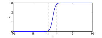
The time-derivative of $\lambda(t)$ is of most interest here as this determines the rate of shift for the (now quasi-) equilibria $x_{\mathrm{eq}}^{(s)}$ and $x_{\mathrm{eq}}^{(u)}$. The time derivative of $\lambda$ is

$$\dfrac{\mathrm{d}\lambda}{\mathrm{d}t}=\dfrac{\epsilon\lambda_{\max}^{2}}{4}\bigg{[}\operatorname{sech}^{2}\bigg{(}\dfrac{\lambda_{\max}\epsilon t}{2}\bigg{)}\bigg{]}=\epsilon\lambda(\lambda_{\max}-\lambda)\mbox{.}$$ (3)

This time derivative reaches its maximum at $t=0$ and so, for a fixed ramp height $\lambda_{\max}$, $\epsilon$ is directly proportional to the maximal rate of shift at $t=0$.

We note that (3) is also an ODE for $\lambda$ such that the prototype model can be considered as a two-dimensional ODE in the $(x,\lambda)$ phase plane (as done by Ashwin et al. (2012)):

$$\dot{x} =f(x,\lambda(t))=(x+\lambda(t))^{2}-1$$ (4)

$$\dot{\lambda} =\epsilon\lambda(\lambda_{max}-\lambda)$$ (5)

Notice that (5) is coupled to (4), but there is no coupling in the other direction.

(a)

(b)

(c)

(d)

(e)

(f)

Figure 2: Time profiles (a),(c),(e) and phase planes (b),(d),(f) of system (4)–(5) for $\epsilon<\epsilon_{c}$ - (a),(b), $\epsilon=\epsilon_{c}$ - (c),(d) and $\epsilon>\epsilon_{c}$ - (e),(f). Black dashed curves are the stable $W^{s}_{0}$ and unstable $W^{u}_{0}$ equilibria in the limit $\epsilon=0$, blue and red curves are the unstable and stable manifolds, $W^{u}(S_{-})$ and $W^{s}(U_{+})$, respectively ($\lambda_{\max}=3$).

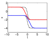
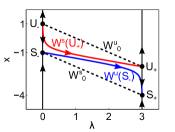
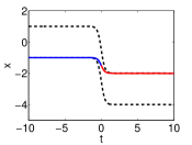
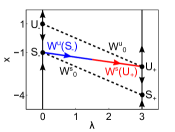
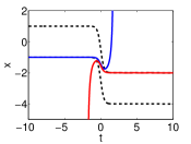
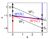
Figure 2 displays all qualitatively different phase portraits possible for (4)–(5) in panels 2(b), 2(d) and 2(f). The system has $4$ equilibria, $S_{-}$ (a saddle) and $U_{-}$ (a source) on the $\lambda=0$ line, and $S_{+}$ (a sink) and $U_{+}$ (a saddle) on the $\lambda=\lambda_{\max}$ line. The upper and lower black dashed lines represent the family of unstable $W^{u}_{0}$ and stable $W^{s}_{0}$ quasi-equilibria in the limit $\epsilon=0$, respectively. The blue curve is the unstable manifold $W^{u}(S_{-})$ of the saddle $S_{-}$, and the red curve is the stable manifold $W^{s}(U_{+})$ of the saddle $U_{+}$. The panels 2(a), 2(c) and 2(e) show the time profiles for $x$ on the invariant manifolds $W^{u}(S_{-})$ and $W^{s}(U_{+})$ (using the same color coding).

One can see that the time profile and the phase portrait of the unstable manifold $W^{u}(S_{-})$ and the stable manifold $W^{s}(U_{+})$ (Figures 2(a) and 2(b)) deviate increasingly from the quasi-equilibrium families $W^{u}_{0}$ and $W^{s}_{0}$ for increasing $\epsilon$. For small $\epsilon$, $W^{u}(S_{-})$ is close to $W^{s}_{0}$, but, for increasing $\epsilon$, $W^{u}(S_{-})$ moves further apart from $W^{s}_{0}$. The unstable manifold $W^{u}(S_{-})$ converges for $t\to\infty$ to the stable node $S_{+}$ for $\epsilon<\epsilon_{c}$. The red curve is the stable manifold $W^{s}(U_{+})$, which forms a separatrix partitioning the plane into two regions. In the region below the separatrix all trajectories are attracted to the stable node $S_{+}$, but in the region above the repelling stable manifold $W^{s}(U_{+})$, all trajectories will escape to $+\infty$ in finite time. Notice that the two manifolds $W^{u}(S_{-})$ and $W^{s}(U_{+})$ are closest at $\lambda=\lambda_{\max}/2$, when the time-derivative $\lambda$ (equation (3)) is at its maximum. This is due to the reflection symmetry within the system (4), (5)

$$\begin{bmatrix}x-x_{c}\\ \lambda-\lambda_{c}\end{bmatrix}\rightarrow\begin{bmatrix}x_{c}-x\\ \lambda_{c}-\lambda\end{bmatrix}$$

around the point $(x_{c},\lambda_{c})=(-1.5,1.5)$.

At a critical $\epsilon$, denoted $\epsilon_{c}$, $W^{s}(U_{+})$ and $W^{u}(S_{-})$ form a heteroclinic connection between the two saddles $S_{-}$ and $U_{+}$, as depicted in Figures 2(c), 2(d). Perryman and Wieczorek (2015) observed that the critical value $\epsilon_{c}$ equals $4/3$ and that the connecting orbit is the line

$$x=-\dfrac{\lambda}{3}-1$$ (6)

in the phase plane. For $\epsilon>\epsilon_{c}$, $W^{u}(S_{-})$ and $W^{s}(U_{+})$ change their arrangement, as displayed by Figures 2(e), 2(f). The unstable manifold $W^{u}(S_{-})$ no longer converges to the stable node $S_{+}$ such that trajectories from all initial conditions close to $S_{-}$ with $\lambda>0$ diverge ($x(t)\to+\infty$). In this case the parameter $\lambda$ is shifted at a rate that is too large for the unstable manifold $W^{u}(S_{-})$ to track the quasi-steady state $W^{s}_{0}$. For $\epsilon>\epsilon_{c}$ but close to $\epsilon_{c}$ this escape does not occur until $\lambda$ is close to $3$ such that one would observe the escape only when $\lambda$ is coming to rest again, and so there appears to be a lag in the timing of escape.

In summary, for this prototype model rate-induced tipping corresponds to a global bifurcation at parameter value $\epsilon_{c}$, a heteroclinic connection from the stable equilibrium before the parameter ramp to the unstable equilibrium after the ramp.

III Delay of early-warning indicators and delay of tipping

For the remainder of this paper we will consider the following scenario: the speed of the parameter ramp $\epsilon$ is less than its critical value $\epsilon_{c}=4/3$ such that without noise the system will not tip. The influence of noise, which we add to the dynamics (4) of $x$, will cause the system to tip with a certain probability. We can control this probability by varying noise intensity and $\epsilon$. We choose our parameters such that an escape of $x$ from $W^{s}_{0}$ beyond $W^{u}_{0}$ to $+\infty$ is extremely unlikely for $t$ far away from $0$ (and, thus, $\lambda$ far away from $\lambda_{\max}/2$). We expect this escape probability to increase during the ramp of $\lambda$ (for $t\approx 0$).

The realizations of $x$ for the prototype system (4)–(5) are governed by the stochastic differential equation (SDE):

$$\mathrm{d}X_{t}=[(X_{t}+\lambda(t))^{2}-1]\mathrm{d}t+\sqrt{2D}\mathrm{d}W_{t}$$ (7)

where $W_{t}$ is standard Brownian motion. The intensity of the noise is given by $\sqrt{2D}$ where $D$ is the diffusion coefficient. The probability density $P(x,t)$ of the random variable $X_{t}$ in the SDE (7) is governed by the Fokker-Planck equation; a linear partial differential equation (PDE):

$$\dfrac{\partial P(x,t)}{\partial t}=D\dfrac{\partial^{2}P(x,t)}{\partial x^{2}}-\dfrac{\partial}{\partial x}\bigg{(}f(x,t)P(x,t)\bigg{)}\mbox{,}$$ (8)

which includes the diffusion coefficient $D$ and drift term $f(x,t)=(x+\lambda(t))^{2}-1$. Applying Dirichlet boundary conditions at some $[x_{\mathrm{start}},x_{\mathrm{end}}]$ will cause the probability density to decay over time as realizations escape the domain. The probability of escape, $p_{\mathrm{esc}}(t_{n})$ at time step $t_{n}$ is therefore defined as:

$$p_{\mathrm{esc}}(t_{n})=1-\frac{\int P(x,t_{n})\mathrm{d}x}{\int P(x,t_{n-1})\mathrm{d}x}$$

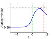
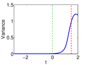
In addition, we use (8) to compute two characteristic quantities of the density $P(x,t)$ for (7), the lag-1 autocorrelation and the variance, shown in Figure 3. These quantities are commonly monitored in time series where one suspects an underlying parameter drift that approaches a bifurcation-induced (specifically saddle-node induced) tipping point. Both, autocorrelation and variance, should increase along the time series as the parameter comes closer to its saddle-node value (see Williamson and Lenton (2015) for other cases such as Hopf bifurcation). But what happens for the rate-induced tipping model?

(a) Autocorrelation

(b) Variance

Figure 3: Traditional early-warning indicators; lag-1 autocorrelation and variance show a delayed response for rate-induced tipping if tipping point is assumed to be at the time $t=0$ (green dashed line), the closest encounter of the stable and unstable manifolds, $W^{u}(S_{-})$ and $W^{s}(U_{+})$. However, both indicators increase before the tipping point if assumed to be at $t\approx 1.5$ (red dashed line) calculated from the peak of the escape rate in Figure 4. Parameters: $\epsilon=1.25$ and $D=0.008$ ($\Delta t=0.01$ for panel 3(a))

The lag-1 autocorrelation $a_{n}$ is defined to be the correlation between successive $X_{n\Delta t}$, separated by a time step $\Delta t$ (we choose $\Delta t=0.01$):

$$a_{n}=\dfrac{\mathrm{Cov}(X_{(n-1)\Delta t},X_{n\Delta t})}{\sqrt{\mathrm{Var}(X_{(n-1)\Delta t})\mathrm{Var}(X_{n\Delta t})}}$$ (9)

where $X_{n\Delta t}$ is the solution of (7) with density $P(\cdot,n\Delta t)$ at time step $n\Delta t$.

The initial condition for (8) is the stationary density of (7) with $\lambda_{0}=\lambda(t_{0})$ restricted to the fixed domain $x\in[x_{\mathrm{start}},x_{\mathrm{end}}]=[-6,2]$, which corresponds to the assumption that the ramp-up of $\lambda$ starts from a stationary state. See Appendix A(a) for a study of dependence on $x_{\mathrm{end}}$. For this stationary starting point the system can be approximately modeled by the Ornstein-Uhlenbeck process

$$\mathrm{d}X_{t}=-\theta X_{t}\mathrm{d}t+\sqrt{2D}\mathrm{d}W_{t}$$

where $\theta=-f^{\prime}(-1,0)=2$ is the decay rate at $S_{-}$. The Ornstein-Uhlenbeck process has autocorrelation and variance given by Aalen, Borgan, and Gjessing (2008):

Autocorrelation: $$a=\exp(-\theta\Delta t)\approx 1-\theta\Delta t$$

Variance: $$V=\dfrac{D}{\theta}$$

where we set $\Delta t=0.01$, thus, giving $a=0.98$ and $V=0.004$ in Figure 3.

We highlight that for starting at $t_{0}=-\infty$ the system will tip with probability one before the ramping shift begins. The time of tipping for a stationary system is approximated by Kramers’ time, $\tau_{K}$ Berglund and Gentz (2004), $(U(x)=-\int f(x)\mathrm{d}x)$:

$$\tau_{K}=C\exp\bigg{(}\dfrac{\Delta U}{D}\bigg{)}$$

where $\Delta U$ is the height of the potential barrier and the prefactor $C$ depends on the curvature at the minimum and maximum of the potential. In our case for equation (7), we have constant values for $\Delta U=4/3$ and $C=\pi$. We consider the regime where the probability of escape from the well, $p_{\mathrm{esc}}(t)$, increases by an order of magnitude during the ramping of the parameter $\lambda$:

$$\frac{1}{\tau_{K}}\ll\max_{t\in\mathbb{R}}p_{\mathrm{esc}}(t)\mbox{.}$$

In this regime we expect the time $t$ for which the escape rate $p_{\mathrm{esc}}(t)$ is maximal to occur at the time $t=0$. This corresponds to the closest encounter of the stable and unstable manifolds, $W^{u}(S_{-})$ and $W^{s}(U_{+})$, due to the symmetry in the deterministic part.

Figure 3 displays the lag-1 autocorrelation and variance for the time interval of most interest, namely $t\in[-3,2]$ when system (4), (5) is non-stationary. We observe that there is a delay in the warning for approaching the tipping point, if we take the tipping point as the time $t=0$ (green dashed line). The autocorrelation (Figure 3(a)) has only just started to increase at $t=0$. The variance (Figure 3(b)) shows an even longer delay in the signal. It increases noticeably only after $t=0$. Ditlevsen and Johnsen (2010) concluded for saddle-node induced tipping that only the presence of both indicators, increase of autocorrelation and variance, is sufficient evidence for the approach of a tipping point. When applied to rate-induced tipping, one would conclude initially that the warning will be significantly delayed from when we would expect the tipping. This warrants a systematic investigation to see when escape is most likely in close encounters with rate-induced tipping.

III.1 Escape rate over time

To investigate when the escape is likely to occur we initially consider the escape rate per unit time calculated using the Fokker-Planck equation (8). The escape rate per unit time is defined as the fraction of realizations that cross a known threshold curve $\tilde{x}(t)$ divided by the time step $\Delta t$. We choose a threshold curve $\tilde{x}(t)$ (bright blue in Figure 4) beyond which we classify a realization as having escaped. The threshold curve is chosen such as $\tilde{x}(t)=x^{u}(t)+y$, where $x^{u}(t)$ is the unique trajectory of the deterministic part of (7) that starts at $x(-10)=x_{0}=-1$ (thus, $(x^{u}(t),\lambda(t))$ is close to $W^{u}(S_{-})$) and $y=1.5$ is a fixed sufficiently large deviation from $x^{u}(t)$. Appendix A.2 studies systematically how the choice of threshold $\tilde{x}(t)$ affects the results.

Figure 4 displays the time profile (4(a)) and the phase portrait (4(b)) of the deterministic trajectory $x^{u}(t)$, the threshold curve $\tilde{x}(t)$ and the escape rate (over time and versus $\lambda$) obtained via (8).

(a) Time profile

(b) Phase plane

Figure 4: Time profile and phase plane and escape rate obtained via (8) for $\epsilon=1.25$ and $D=0.008$. Dashed curves represent stable $W^{s}_{0}$ and unstable $W^{u}_{0}$ equilibria, the dark blue curve is the unstable manifold $W^{u}(S_{-})$, the bright blue curve is the threshold curve $\tilde{x}(t)$ for $y=1.5$.

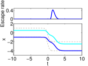
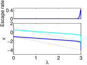
In this example, we have chosen $\epsilon=1.25$, which is close to $\epsilon_{c}=4/3$, and a small noise level $D=0.008$. For this choice of ramping speed parameter $\epsilon$, tipping would not occur in the deterministic case ($D=0$). However, with a noise level of $D=0.008$, roughly $36\%$ of realizations that start with initial condition $x(-10)=x_{0}$ go on to escape. As in Figure 2, the dark blue curve is the unstable manifold $W^{u}(S_{-})$ (the deterministic solution $x^{u}(t)$, starting at $x(-10)=x_{0}$, is extremely close to it). The bright blue curve is our threshold curve $\tilde{x}(t)$ (see Figure 13 in Appendix A.2 how the escape time depends on the threshold).

Figure 4 shows that the escape is most likely to occur at about $t=1.5$, hence, it is delayed, too. The red dashed line in Figure 3 represents the most likely time of tipping, given by the peak of the escape rate in Figure 4. Therefore taking this as our tipping point we see that there is an increase in both the autocorrelation and the variance on the approach to tipping. We conclude that for this example at least that the tipping is delayed and thus the early-warning signals can still offer forewarning of rate-induced tipping.

For a systematic study of how the time of most likely escape depends on the system parameters we formulate a variational optimization problem for the optimal path of escape.

IV Most likely (optimal) escape paths — The general variational problem

In this section we will formulate the ODE boundary-value problem (BVP) determining locally most likely paths for escape.

We define the most likely escape path as the path going from given $x_{0}$ to a given $x_{T}$ in a time interval $[t_{0},T_{\mathrm{end}}]$ maximizing the functional

$$F=\exp \bigg{[}\dfrac{U_{0}-U_{T}}{2D}-\int_{t_{0}}^{T_{\mathrm{end}}}\bigg{(}\dfrac{\dot{x}^{2}}{4D}+V_{s}\bigg{)}\mathrm{d}t\bigg{]}$$ (10)

along the path. The terms in $F$ are

$$U(x,t) =-\int f(\bar{x},t)\mathrm{d}\bar{x}\mbox{,}$$

$$V_{s}(x,t) =\dfrac{1}{4D}\bigg{(}\dfrac{\partial U}{\partial x}\bigg{)}^{2}-\dfrac{1}{2}\dfrac{\partial^{2}U}{\partial x^{2}}-\dfrac{1}{2D}\dfrac{\partial U}{\partial t}\mbox{,}$$ (11)

$$U_{0} =U(x_{0},t_{0})\mbox{,}\quad U_{T}=U(x_{T},T_{\mathrm{end}})\mbox{.}$$

The quantity $U$ is the potential of the deterministic part $f$ of the SDE (7) such that (7) can be written in terms of $U(x,t)$:

$$\mathrm{d}X_{t}=-\dfrac{\partial U(X_{t},t)}{\partial X_{t}}\mathrm{d}t+\sqrt{2D}\mathrm{d}W_{t}\mbox{.}$$ (12)

For a differentiable path $x$ the functional $F$ equals the probability of a realization $X_{t}$ following a sequence of infinitesimally small intervals $[x(k\Delta t)-\delta/2,x(k\Delta t)+\delta/2]$ in the limit $0<\delta\ll\Delta t\ll 1$ (up to a constant factor independent of $x$). Recall, that the random variable $X_{t}$ had a probability density function $P(x,t)$ given by the linear Fokker-Planck equation (8), from which the functional $F$ is derived. See Zhang (2008), (p. 25-31) for a detailed derivation of the functional $F$ from equations (10)-(12) for a time independent potential $U(x)$ (a simple extension is made for a time dependent potential $U(x,t)$ in Lin and Ho (2011) and Ho and Dai (2008)).

Assuming a fixed time interval $[t_{0},T_{\mathrm{end}}]$ and fixed start and end points $x_{0}$ and $x_{T}$, local critical points of $F$ are given by the Euler-Lagrange equation, a 2nd order BVP Zhang (2008):

$$\ddot{x}=2D\dfrac{\partial V_{s}}{\partial x}(x,t)\mbox{,}\qquad\begin{cases}x(t_{0})&=x_{0}\mbox{,}\\ x(T_{\mathrm{end}})&=x_{T}\mbox{.}\end{cases}$$ (13)

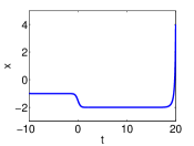
We would like to point out that the BVP (13) used to calculate the locally optimal path is valid for a scalar time-dependent system and for finite (non-small) noise variance $2D$. In the small noise limit, one can use minimum action methods to find the optimal path, which can be applied to multiple dimensions Ren, Vanden-Eijnden et al. (2004). Furthermore, according to Ren, Vanden-Eijnden et al. (2004), in gradient systems, over an infinite time interval, the optimal path becomes a minimum energy (where ‘energy’ refers to the functional $F$ that is optimized) path that forms a heteroclinic orbit between the two local minima of the potential. However, Figure 5 demonstrates that even for relatively small noise levels $D$ (such as $D=0.008$ as chosen for previous illustrations) we are far away from the small noise limit such that $T_{\mathrm{end}}$ is of order $1$: Figure 5(a) shows the (locally) optimal path $x(t)$ for $T_{\mathrm{end}}=20$. We observe that for a long time ($1<t<18$) the path $x(t)$ stays close to the saddle $U_{+}$ before eventually escaping to the chosen $x_{T}=4$. As Figure 5(b) shows, the lingering of $x(t)$ close to the saddle is only optimal for the fixed large $T_{\mathrm{end}}=20$. The functional $M=\log(F)$ increases for decreasing $T_{\mathrm{end}}$.

This implies that for positive (even small) noise variance $2D$ the functional $F$ should also be optimized with respect to the traveling time $T_{\mathrm{end}}$ of the path. We formulate the extended BVP corresponding to critical points with respect to path and traveling time in rescaled time on the base interval $[0,1]$. The BVP will then be solved with standard continuation software AUTO Doedel (2007). The BVP (13), rescaled to $[0,1]$ is (split into two components):

$$\dot{x}_{1} =x_{2}(T_{\mathrm{end}}-t_{0})\mbox{,} x_{1}(0) =x_{0}\mbox{,}$$ (14)

$$\dot{x}_{2} =g(x_{1},t)(T_{\mathrm{end}}-t_{0})\mbox{,} x_{1}(1) =x_{T}$$ (15)

where $t_{0}$ (fixed) and $T_{\mathrm{end}}$ (free) are the start and end $t$ values and

$$g(x_{1},t)=2D\dfrac{\partial V_{s}}{\partial x}(x_{1}(t),t)\mbox{.}$$

The solution of (14)–(15) is a critical point of $F$, given in (10), among all possible paths connecting from $x_{0}$ to $x_{T}$ in a fixed time $T=T_{\mathrm{end}}-t_{0}$. The function $M=\log(F)$, written for the rescaled path is

$$M=\int\limits_{0}^{1}\dfrac{U_{0}-U_{T}}{2D}-\bigg{[}\dfrac{x_{2}(t)^{2}}{4D}+V_{s}(x_{1}(t),t)\bigg{]}(T_{\mathrm{end}}-t_{0})\mathrm{d}t$$ (16)

$$\mbox{where}\quad U_{0}=U(x_{0},t_{0})\mbox{,}\quad U_{T}=U(x_{T},T_{\mathrm{end}})\mbox{.}$$

(a)

(b)

Figure 5: (a) Optimal path for $T_{\mathrm{end}}=20$. (b) Plot of function $M$ that needs to be maximized w.r.t. $T_{\mathrm{end}}$. $t_{0}=-10$, $\epsilon=1.25$, $D=0.008$.

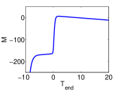
Paths maximizing $F$ (and, hence, $M$) also maximize the probability of realizations of SDE (7) following it. Figure 5(b) plots $M$ along paths satisfying (14)–(15) for a range of end times $T_{\mathrm{end}}$. Its maximum corresponds to the time $T_{\mathrm{end}}$ for which the functional $M$ is (locally) maximal among the range of $T_{\mathrm{end}}$ shown (this is for the fixed positive but small noise variance $2D=0.016$). We now extend the BVP (14)–(15) to include the criticality of $T_{\mathrm{end}}$ into the optimization problem. We outline the BVP of the variational problem for the general case here. The specific case for this example is in Appendix B.

Introducing the derivatives of $x_{1}$ and $x_{2}$ w.r.t. $T_{\mathrm{end}}$ as

$$z_{1}(t)=\dfrac{\partial x_{1}(t)}{\partial T_{\mathrm{end}}},\qquad z_{2}(t)=\dfrac{\partial x_{2}(t)}{\partial T_{\mathrm{end}}}\mbox{,}$$

these derivatives satisfy

$$\begin{aligned} \dot{z}_{1}&=x_{2}+z_{2}(T_{\mathrm{end}}-t_{0})\mbox{,}&z_{1}(0)&=0\mbox{,}\\ \dot{z}_{2}&=g(x_{1},t)+\dfrac{\partial g(x_{1},t)}{\partial x_{1}}z_{1}(T_{\mathrm{end}}-t_{0})\mbox{,}&z_{1}(1)&=0\mbox{.}\end{aligned}$$ (17)

Critical points of $M(x_{0},t_{0},x_{T},T_{\mathrm{end}},x_{1}(\cdot),x_{2}(\cdot))$, given in equation (16), w.r.t. $T_{\mathrm{end}}$ satisfy

$$\dfrac{\partial M}{\partial T_{\mathrm{end}}}+\dfrac{\partial M}{\partial x_{1}}\dfrac{\partial x_{1}}{\partial T_{\mathrm{end}}}+\dfrac{\partial M}{\partial x_{2}}\dfrac{\partial x_{2}}{\partial T_{\mathrm{end}}}=0\mbox{,}$$

which produces the integral condition:

$$0=m:=\int\limits_{0}^{1}\bigg{[}\dfrac{1}{2D}\dfrac{\partial U(x_{T},T_{\mathrm{end}})}{\partial T_{\mathrm{end}}}+\dfrac{x_{2}(t)^{2}}{4D}+V_{s}(x_{1}(t),t)\\ +\bigg{(}\dfrac{x_{2}(t)z_{2}(t)+g(x_{1}(t),t)z_{1}(t)}{2D}\bigg{)}(T_{\mathrm{end}}-t_{0})\bigg{]}\mathrm{d}t$$ (18)

Therefore, have to solve the four-dimensional BVP (14), (15), (17) for $x_{1}(t)$, $x_{2}(t)$, $z_{1}(t)$, $z_{2}(t)$ with the additional integral condition (18) and the additional parameter $T_{\mathrm{end}}$. We use AUTO (Version: AUTO-07P) Oldeman, Doedel, and Paffenroth (2013) to study the solutions of (14), (15), (17), (18) in dependence of the system parameters $D$ and $\epsilon$.

V Sequence of continuation steps for the optimal path to escape in optimal time

Since (14), (15), (17), (18) is nonlinear we need a sequence of initialization steps to arrive at the optimal path for particular desired values of ramping speed parameter (initially $\epsilon=1.25$, close to critical value $\epsilon_{c}=4/3$) and noise variance (initially $2D=0.1$). An advantage of using continuation is that once we have obtained an optimal path in an optimal time for a particular set of parameters we are free to perform a systematic parameter study of solutions of (14), (15), (17), (18) varying the ramping speed $\epsilon$ and noise level $D$.

V.1 List of free parameters

First we discuss some of the parameters used and reasoning for their initial values, as given in Table 1.

Table 1: Types of parameters used in continuation steps and their initial values

System (fixed) parameters	Continuation parameters	Bifurcation parameters	Monitoring parameter
$\!\begin{aligned} \ \\[-12.91663pt] p&=1\\ \lambda_{\max}&=3\\ t_{0}&=-10\\ x_{0}&=-1\end{aligned}$	$\!\begin{aligned} \ \\[-12.91663pt] T_{\mathrm{init}}&=0\\ x_{T}&=x_{0}\\ T_{\mathrm{end}}&=-9\\ m&=m_{0}\end{aligned}$	$\!\begin{aligned} \ \\[-12.91663pt] \epsilon&=1.25\\ D&=0.05\\ \\ \\ \end{aligned}$	$\!\begin{aligned} \ \\[-12.91663pt] M&=M_{0}\\ \\ \\ \\ \end{aligned}$

We introduce the factor $T_{\mathrm{init}}$ in equation (15) as an artificial parameter. Thus, (14)–(15) changes to

$$\dot{x}_{1} =x_{2}(T_{\mathrm{end}}-t_{0})$$

$$\dot{x}_{2} =g(x_{1},t)(T_{\mathrm{end}}-t_{0})T_{\mathrm{init}}\mbox{,}$$

giving a trivial system ($\dot{x}_{1}=x_{2}(T_{\mathrm{end}}-t_{0})$, $\dot{x}_{2}=0$) for $T_{\mathrm{init}}=0$, connecting it to system (14)–(15) via a continuation in $T_{\mathrm{init}}$ from $0$ to $1$. Furthermore, we initially choose $x_{T}=x_{0}$ and $T_{\mathrm{end}}=t_{0}+1=-9$, close to the initial time value $t_{0}$. Finally, the parameters $M$ and $m$ are used to monitor the values of the integrals in equations (16) and (18), respectively, such that sign changes of $m$ correspond to critical values of the functional $M$ (and, hence, $F$). The initial values of $M$ and $m$ are set equal to the integrals in (16) and (18) along the initial path. Outlined in Table 2 is a brief summary of the continuation steps performed to create an optimal path in an optimal time. We proceed with a brief explanation for each of the continuation steps with a more in depth discussion provided in Appendix C.

Table 2: Summary of continuation steps to perform in order to achieve an optimal path for escape in an optimal time (in brackets are the values used)

Step $\#$	Continuation parameter	Initial value	End value	Other free parameters
1	$T_{\mathrm{init}}$	$(0)$	$(1)$	$m$, $M$
2	$x_{T}$	$x_{0}$ $(-1)$	$\gg 1$ $(4)$	$m$, $M$
3	$T_{\mathrm{end}}$	$\sim t_{0}$ $(-9)$	$\gg 1$ $(20)$	$m$, $M$

V.2 Step 1: continuation of $T_{\mathrm{init}}$ from $0$ to $1$

The first step ends in a solution of the full system of equations (14)-(15). This is the short orbit (blue) from $x_{1}=S_{-}=-1$ to $x_{1}=-1$ in Figure 6. The parameters $M$ and $m$ are kept free during the continuation, monitoring the integrals in (16) and (18).

V.3 Step 2: continuation in $x_{T}$

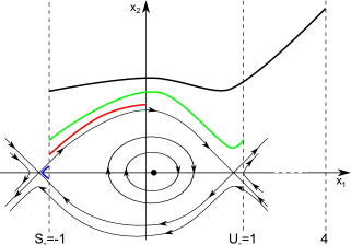
The result of Step 1 is a path maximizing $M$ when traveling from $x_{0}=-1$ to $x_{T}=-1$ in unit time ($t_{0}=-10$, $T_{\mathrm{end}}=-9$), where $\lambda(t)$ is close to stationary ($\lambda\approx 0$). Step 2 changes the right boundary value $x_{T}$ to the desired location. Guided by our aim to find most likely paths for escape, we perform a continuation to $x_{T}=4$ (we count a trajectory of (7) that reaches $x_{T}=4$ as having escaped). Figure 6 shows a sequence of solutions of (14)–(15) (colored) for the continuation stages of $x_{T}$ superimposed onto the phase portrait of the system (14)–(15) for $\lambda=0$.

Figure 6: Illustration of trajectories (colored) at different stages of the $x_{T}$ continuation step superimposed on the phase portrait for the full rate-induced system, when stationary, $\lambda=0$. $x_{T}=x_{0}=-1$ (blue), $x_{T}=0$ (red), $x_{T}=1$ (green), $x_{T}=4$ (black).

The results of this step is a path maximizing $M$ that connects $x_{0}=-1$ and $x_{T}=4$ in a very short time period ($T_{\mathrm{end}}-t_{0}=1$, see Figure 14(b) in Appendix C.2). Clearly this is not the optimal time to make this transition and so the next step is to continue in $T_{\mathrm{end}}$ to get to more realistic timings of escape.

V.4 Step 3: continuation in $T_{\mathrm{end}}$

We increase $T_{\mathrm{end}}$ to a large value, monitoring $M$ and $m$. Figure 5(b) shows the graph of $M$ over $T_{\mathrm{end}}$, which has a pronounced maximum at $T_{\mathrm{end}}\approx 1.5$. Critical points of $M$ are detected when $m$ changes sign, and therefore gives the optimal path for an optimal time provided $M$ is a maximum.

The optimal path constructed by the above steps will be systematically continued in the system parameters $D$ (noise variance $2D$) and $\epsilon$ (ramping speed of $\lambda(t)$) in Section VII.

VI Optimal path for escape for noise and rate-induced tipping

This section compares the optimal path for escape with the escape calculated directly from the solutions of (8). We are interested in the timing of escape, defined as the timing of crossing certain threshold curves. We do not want to have to rely on running full Monte Carlo simulations, but instead use the optimal path theory developed by Chaichian and Demichev (2001); Zhang (2008). We include the optimal path for escape (in green) into Figure 4 to compare the most likely timing of escape (the peak in the escape rate, measured at the threshold $\tilde{x}$) with the time $t$ the threshold $\tilde{x}$ intersects with the optimal path as computed through continuation, see Figure 7. The corresponding phase portrait in Figure 7(b) shows that both the simulations and optimal path suggest that the escape does not happen until just short of $\lambda=3$, the moment the potential well or steady states $W^{s}_{0}$, $W^{u}_{0}$ are coming to a rest.

(a) Time profile.

(b) Phase plane.

Figure 7: Time profile and phase plane with escape rate from simulations (top) and optimal path added in green for $\epsilon=1.25$ and $D=0.008$. Dashed curves represent stable $W^{s}_{0}$ and unstable $W^{u}_{0}$ quasi-equilibria, the dark blue curve is the unstable manifold $W^{u}(S_{-})$, the bright blue curve is the threshold curve $\tilde{x}(t)=x^{u}(t)+y$ with $y=1.5$.

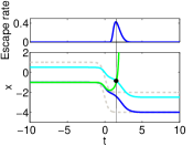
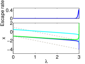
Figure 7 illustrates that the optimal path matches the mode (peak) of the escape rate well. In general, if the escape rate over time is unimodal with a sharp peak then the time profile of the optimal path is a good description of this peak. More precisely, the mode of the escape rate occurs very close to a time $t$ for which $\tilde{x}=x_{1}(t)$, where $x_{1}$ is the first component of the optimal path, the solution of the extended BVP (14), (15), (17), (18).

VI.1 Dependence on choice of threshold curve $\tilde{x}(t)$:

The choice of the threshold curve $\tilde{x}(t)$ in Figure 7 is at $\tilde{x}(t)=x^{u}(t)+y$ with $y=1.5$ (recall that $x^{u}(t)$ is the trajectory of the deterministic part of (7). Figure 8 shows a color plot for the escape rate at the threshold depending on the distance $y$. The distance of the optimal path from the unique trajectory $x^{u}(t)$ added in white. This highlights that, provided the threshold $\tilde{x}(t)$ is sufficiently far from $x^{u}(t)$, the optimal path will cross the threshold at the same moment the escape rate through the threshold is at its peak.

Figure 8: Color plot of the escape rate at the threshold $\tilde{x}(t)$ depending on the distance $y$ from the unstable manifold $W^{u}(S_{-})$. Distance of optimal path from $x^{u}(t)$ added in white, $\epsilon=1.25$, $D=0.008$.

VI.2 Dependence on starting time $t_{0}$ and starting position $x_{0}$:

We emphasize that the optimal path calculates the local optimum, i.e. assuming the system has not tipped before the ramping shift begins. We set $t_{0}=-10$, $x_{0}=-1$ to represent starting at the bottom of the potential well at time $-\infty$. Changing the starting time, for example to $t_{0}=-15$ or $t_{0}=-5$ has no effect on when the optimal path escapes and only extends or shortens the time profile of the path presented in Figure 7(a). Likewise, changing the starting position, provided it is still inside the well, has no effect on when the optimal path escapes. For slightly different $x_{0}$ the optimal path will converge onto the path in Figure 7(a) before $t=0$ and then follow the same path for escape.

Figure 9 shows how the $x_{1}(t)$ component of the optimal path is connected to the evolution of the density of realizations.

(a) Time profile.

(b) Phase plane.

Figure 9: Time profile and phase plane for density plot of simulations and optimal path added in bright blue for $\epsilon=1.25$ and $D=0.008$. Dashed white curves represent stable and unstable equilibria.

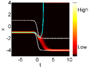
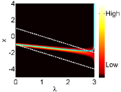
In the time profile plot, initially the spread of the distribution is very narrow centered around the steady state $W^{s}_{0}$, due to the small noise level $D$. When the system shifts, this distribution widens reflected by a lower density over a larger $x$ range. Once the shift stops, the density gradually becomes concentrated again, but some realizations have escaped, indicated by the elevated density at $x=4$. Initially, the optimal path is right at the mean of the distribution. The time when the optimal path deviates from the mean equals the time the density in the simulation is at its widest and where the additional mode (at $x=4$) appears. This once again suggests that the optimal path, derived from BVP (14), (15), (17), (18), describes the escape of realizations of the stochastic differential equation (7).

VII Timing of escape in 2 parameter plane

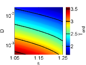
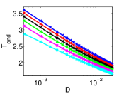
One of the advantages of reducing the study of escape time to optimal paths is that we can perform a systematic parameter study with moderate computational effort. First, we investigate the timing of escape in the two parameter plane of the ramping speed $\epsilon$ and noise level $D$, Figure 10, panels 10(a), 10(c) and 10(e). Panel 10(a) indicates with a black marker the end time $T_{\mathrm{end}}$ at which a particular optimal path reaches the end position $x_{T}=4$. Panel 10(c) shows a color contour plot, with the color denoting the time $T_{\mathrm{end}}$ for a range of optimal paths dependent on the ramping speed $\epsilon$ and noise level $D$. Recall that the optimal path is calculated by solving the system of equations (14)-(18) and following the continuation steps outlined in Section V for a particular $\epsilon$ and large noise level $D$. Then for each $\epsilon$ a final continuation is performed over $D$ to create an $11\times 40$ grid for the color plot.

The optimal path begins at $t_{0}=-10$ and so the length of the time interval for the path is between $11.7$ and $13.5$ time units for this range of $\epsilon$ and $D$ values. This demonstrates that for a small $\epsilon$ value and small noise levels escape occurs for positive $T_{\mathrm{end}}$, that is, with a delay compared to the time of closest encounter of the deterministic manifolds $W^{u}(S_{-})$ and $W^{s}(U_{+})$ (which would be at $t=0$). As $\epsilon$ increases towards $\epsilon_{c}=4/3$ and the noise level increases the time to escape decreases. This can be seen more clearly in panel 10(e), which takes cross sections of panel 10(c) for different values of $\epsilon$. The relationship is almost linear between the logarithm of the noise level and the time at which the final destination $x_{T}$ is reached. In summary, panels 10(c) and 10(e) indicate that the escape occurs with a delay especially for small noise. To investigate the precise value of the delay we will look at the timing of intersection between the optimal path and the stable manifold $W^{s}(U_{+})$, indicated by the black marker in panel 10(b).

(a)

(b)

(c)

(d)

(e)

(f)

Figure 10: Plots for end time $T_{\mathrm{end}}$ (a),(c),(e) and the crossing time $t_{\mathrm{cross}}$ with the stable manifold $W^{s}(U_{+})$ (b),(d),(f) of the optimal path (solution of (14)-(18)) for escape. (a),(b) Time profile of optimal path (green) and stable manifold $W^{s}(U_{+})$ (red) with the black marker highlighting $T_{\mathrm{end}}$ (a), $t_{\mathrm{cross}}$ (b) for a particular optimal path ($\epsilon=1.25$, $D=0.008$). (c),(d) Color contour plots for end time $T_{\mathrm{end}}$ (c) and the crossing time $t_{\mathrm{cross}}$ (d) in the 2 parameter $(\epsilon,D)$ - plane. (e),(f) Cross sections of (c),(d) respectively where each contour represents different value of $\epsilon$, spaced evenly at $0.04$ intervals, starting with $\epsilon=1.05$ (dark blue, top) increasing to $\epsilon=1.25$ (bright blue, bottom).

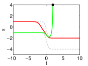
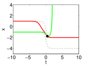
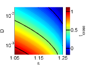
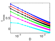
The reason for considering the stable manifold $W^{s}(U_{+})$ as a threshold is that it plays a role similar to a saddle in stationary escape problems. Once a realization has crossed this threshold it is more likely to escape to $+\infty$ (in finite time in our example). One may expect the optimal (that is, most likely) escape path to cross this manifold when the two manifolds $W^{u}(S_{-})$ and $W^{s}(U_{+})$ are closest together at $t=0$. The question is then whether the escape across the stable manifold $W^{s}(U_{+})$ occurs at $t$ close to $0$. Panels 10(d) and 10(f) present the timing of crossing the stable manifold $W^{s}(U_{+})$ to establish if this is the case.

We observe that the range of crossing times is smaller than the range of end times to reach $x_{T}$($=4$). This is expected since the traveling time from $W^{s}(U_{+})$ to $x_{T}$ decreases for increasing noise level $D$. For small noise levels the optimal path tracks the manifold $W^{s}(U_{+})$ for longer. In the limit of large noise level $D$ in the $(\epsilon,D)$-parameter plane the most likely crossing time is $t_{\mathrm{cross}}\approx t_{0}$(not shown). In this limit we have a purely noise-induced transition as the potential is nearly stationary at $t_{0}$. For decreasing $D$ the intersection between the optimal path and stable manifold $W^{s}(U_{+})$ varies with different ramping speeds $\epsilon$ such that we have combination of noise and rate-induced tipping, with timing depending on both parameters. As the ramping speed $\epsilon$ and noise level $D$ decreases the crossing time delay $t_{\mathrm{cross}}$ increases. For the smaller noise levels in the computed range the intersection $t_{\mathrm{cross}}$ of the optimal path with the stable manifold $W^{s}(U_{+})$ is of order $1$, when the manifolds $W^{u}(S_{-})$ and $W^{s}(U_{+})$ are significantly further apart than at $t=0$. This justifies the claim in the abstract that for noise- and rate-induced tipping the escape is delayed in the small noise limit.

(a) Color contour.

(b) Cross section.

Figure 11: (a) Color plot of the value of $M$. (b) Cross section of (a) each contour represents different value of $\epsilon$, spaced evenly at $0.04$ intervals, starting with $\epsilon=1.05$ (dark blue, bottom) increasing to $\epsilon=1.25$ (bright blue, top).

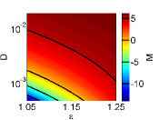
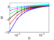
Figure 11 gives a crude estimate for the probability of escape depending on the ramping speed $\epsilon$ and noise level $D$. Note though, these are not the true probabilities but rather the values of the functional $M=\log F$ (see (10)) which the most likely path optimizes. The color in Figure 11(a) in the 2 parameter $(\epsilon,D)$-plane equals the value of the functional $M$ along the optimal path found at the corresponding point in the $(\epsilon,D)$-plane. As expected, the largest probability of escape is for large ramping speeds and large noise levels. The value of $M$ is smallest for slow ramping speeds and low noise levels. Figure 11(b) displaying the cross section of Figure 11(a) for different values of $\epsilon$ illustrates that $M$ decreases logarithmically as $D$ decreases on a logarithmic scale.

VIII General delay of tipping

In Section VII, we have shown that the tipping is delayed especially for small noise levels. In the context of autonomous systems Bakhtin (2013) gives an asymptotic formula for this delay. Bakhtin (2013) considers rare escapes for small noise levels for a process $\mathrm{d}x=xf(x)+\sqrt{2D}\mathrm{d}W_{t}$ on the interval $[A,B]$ containing $0$, starting from $x_{0}<0$, where $f$ is uniformly positive. Then the first time $T=T_{\mathrm{end}}-t_{0}$ to exit at the point $B$ (under the condition that $x(t)$ does indeed exit at $B$) in the limit $\sqrt{2D}\rightarrow 0$ satisfies

$$T=c_{1}\ln\bigg{(}\dfrac{1}{\sqrt{2D}}\bigg{)}$$

where $c_{1}$ is a constant independent of $D$. This states that for an autonomous system, the time for rare escapes increases linearly as the noise level decreases exponentially. This is consistent with our findings for the non-autonomous system, that as the noise is decreased the time $t_{\mathrm{cross}}$ at which the optimal path crosses the stable manifold $W^{s}(U_{+})$ increases slowly, Figure 10(f). To conclude, we find a similar relationship for the delay in the rate-induced tipping as that of Bakhtin (2013) for rare escapes of an autonomous system. The observed level of delay in Section VII is of order $1$ such that the noise levels that we consider small in Section VII are still far larger than the small-noise limit, for which BVPs for optimal escape paths are available in arbitrary dimensions. (These paths tend to be connecting orbits such that the optimal time is always infinity)Ren, Vanden-Eijnden et al. (2004).

IX Conclusions

We have shown that two commonly used early-warning indicators of tipping (increase of autocorrelation and increase of variance) are present but delayed in a prototypical model of rate-induced tipping. By looking at the timing of escape using optimal paths we find that the tipping event itself is delayed for small noise levels. We conclude that the delay in the early-warning indicators is consistent with the delay in the actual tipping (at least for the example).

We extended the boundary-value problem for the most likely path for tipping (escape) based on Zhang (2008) to include optimality of time for finite noise. This additional optimality criterion created a variational optimization problem that we solved computationally with continuation techniques (using the package AUTO). With the help of continuation we performed a systematic parameter study in the $(\epsilon,D)$-plane (ramping speed vs. noise level). The time when the optimal path for escape crosses the stable manifold $W^{s}(U_{+})$ is a measure for the timing of tipping. We find that for large ramping speeds and noise levels there is no delay and even for lower ramping speeds there is only a small delay. However, for small noise levels $D$ the tipping delay is of order $1$.

We hypothesize that the observed delay in tipping is present independent of the particular form of $\lambda(t)$ as long as it is qualitatively similar to the ramp like shift (3). Similarly, this delay should be observable independent of the particular shape of the potential well $U(\cdot,t)$. This paper demonstrated that the optimal path for escape, a solution of a BVP, matches simulation results well. The technique used to find the optimal path of escape finds the local maximum and is general such that it can be used to determine the timing for any type of tipping.

However, the optimal path may miss the global optimum when there is more than one realistic opportunity for escape. For a small single window of escape as considered in this paper the escape rate will form a unimodal distribution with a narrow peak, for which the optimal path is close to the mode. However, if one considers different scenarios $\lambda(t)$ for ramping the system parameter (for example, one that is not monotonically increasing, see Ashwin, Perryman, and Wieczorek (2015)), the escape rate would have a multimodal distribution. We conjecture that we find one optimal path for each of the modes of the distribution. It is unclear if for non-monotone parameter shift $\lambda(t)$ the tipping or the early-warning indicators are delayed for the small noise levels. This would further support the conclusion that the autocorrelation and variance can be used as early-warning signals for rate-induced tipping events. Furthermore, this paper has focused on the one-dimensional case. Thus, an extension to the general multiple dimensional case is still required.

Appendix A Dependence on parameters

This appendix details how the choice of the parameters $x_{\mathrm{end}}$, the upper domain boundary, and the threshold parameter $y$ affects the results presented in the paper.

A.1 Domain boundary parameter

We investigate the effect the upper boundary of the domain, $x_{\mathrm{end}}$, has on the early-warning indicators, the increase of autocorrelation and variance. We choose a domain $[x_{\mathrm{start}},x_{\mathrm{end}}]$ with $x_{\mathrm{start}}=-6$ and $x_{\mathrm{end}}$ as shown in Figure 12. Choosing the domain fixed in time is natural as in realistic problems we do not know a-priori the location of the moving well. In Section III we chose $x_{\mathrm{end}}=2$, which corresponds to a wide domain for the problem (including realizations into the computation of the early-warning indicator, which are already escaping). Figure 12 explores the effect narrowing the domain has on the decay rate estimate $\theta=(1-a)/\Delta t$ (where $a$ is the lag-$1$ autocorrelation with time step $\Delta t$) and variance $V$. We consider the decay rate, instead of the linearly related autocorrelation as the decay rate is independent of the time step $\Delta t$.

(a) Decay rate

(b) Variance

Figure 12: Effect of the width of domain on the decay rate and variance by varying upper boundary $x_{\mathrm{end}}$

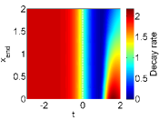
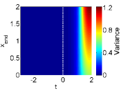
In Figure 12(a), we see that the timing of the onset of the decrease of the decay rate estimate $\theta$ is independent of the upper boundary of the domain, $x_{\mathrm{end}}$, and hence, so is timing of the onset of the increase of the lag-$1$ autocorrelation $a$. Likewise, in Figure 12(b) the timing of the onset of the variance is independent of $x_{\mathrm{end}}$ and, importantly, shows no increase before $t=0$. The precise values of the autocorrelation and the variance depend, of course, strongly on the width of the domain (and, hence, on $x_{\mathrm{end}}$). Thus, we have shown that, while autocorrelation and variance change quantitatively with the domain width, the timing of their increase (which is the early-warning indicator) does not change.

A.2 Threshold parameter

This section presents in more detail how the distance $y$ of the threshold curve $\tilde{x}(t)$ (at which we consider a realization as escaped) from the deterministic trajectory $x^{u}(t)$ influences our results ($\tilde{x}(t)=x^{u}(t)+y$). If we choose $y$ too small, then escape will be detected everywhere. This is demonstrated by Figure 13. For example, when the steady state is stationary no escape should be detected, because, if realizations cross the threshold $\tilde{x}(t)$, most will not escape to $+\infty$ but will return to the unstable manifold $W^{u}(S_{-})$. Clearly for a larger noise level $D$ a greater $y$ is required as there will be larger fluctuations about the unstable manifold $W^{u}(S_{-})$ than for a small noise level.

(a) $D=0.1$

(b) $D=0.008$

Figure 13: Evaluating distance $y$ required between the deterministic trajectory $x^{u}(t)$ and threshold $\tilde{x}(t)$ in both the large and small noise limit cases, $\epsilon=1.25$

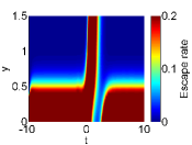
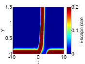
Figure 13(a) demonstrates that for values of $y$ less than a critical value $y_{c}\approx 1$, a large fraction of realizations would count as escaped even for $t$ close to $\pm 10$, where $\lambda$ is close to stationary, in the large noise case. For smaller noise level Figure 13(b) illustrates that a smaller $y$ will suffice. Both figures show that above a certain minimal value of $y$ the window of escape remains nearly independent of $y$. The value $y=1.5$, used in Section VI for our threshold curve $\tilde{x}(t)$, is well above that minimal value of $y$.

Appendix B Variational optimization problem for specific example

The following is the variational optimization problem for the specific rate-induced example discussed in the paper, equation (7).

The potential $U(x,\lambda(t))$ for equation (7) is:

$$U(x,\lambda(t)) =-\dfrac{x^{3}}{3}-\lambda x^{2}+(1-\lambda^{2})x\mbox{\quad such that}$$

$$U^{\prime} =-x^{2}-2\lambda x+1-\lambda^{2}$$

$$U^{\prime\prime} =-2(x+\lambda)$$

$$\dot{U} =-\dot{\lambda}x(x+2\lambda)=-\epsilon\lambda x(\lambda_{\max}-\lambda)(x+2\lambda)$$

where $U^{\prime}$ and $\dot{U}$ represent the derivatives of the potential w.r.t. space and time respectively and $\dot{\lambda}$ is given by equation (5). These equations feed into the $V_{s}$, equation (11) giving:

$$V_{s}= \dfrac{x^{4}+4\lambda^{2}x^{2}+(1-\lambda^{2})^{2}+4\lambda x^{3}-2x(x+2\lambda)(1-\lambda^{2})}{4D}$$

$$+x+\lambda+\dfrac{\epsilon\lambda x(\lambda_{\max}-\lambda)(x+2\lambda)}{2D}$$

and so the 2nd order boundary value problem, equation (13), split into 2 first order ODEs augmented with the ODE for $\lambda$, equation (5), which are to be solved on the $[0,1]$ time domain in AUTO looks like:

$$\dot{x}_{1} =x_{2}(T_{\mathrm{end}}-t_{0})$$ (19)

$$\dot{x}_{2} =h_{2}(x_{1},\lambda(t))(T_{\mathrm{end}}-t_{0})$$ (20)

$$\dot{\lambda} =h_{3}(\lambda(t))(T_{\mathrm{end}}-t_{0})$$ (21)

where (19)-(21) correspond with (14)-(15) and

$$h_{2}(x_{1},\lambda(t)) =2D\dfrac{\partial V_{s}(x_{1},\lambda(t))}{\partial x_{1}}$$

$$h_{3}(\lambda(t)) =\epsilon\lambda(\lambda_{\max}-\lambda)$$

The function $M=\log(F)$, equation (16) for the general case, is maximized and used to monitor any maxima or minima, is given by:

$$M= \int_{0}^{1}\bigg{[}\dfrac{U(x_{0},\lambda(t_{0}))-U(x_{T},\lambda(T_{\mathrm{end}}))}{2D}$$ (22)

$$-\bigg{(}\dfrac{x_{2}}{4D}+V_{s}(x_{1},\lambda(t))\bigg{)}(T_{\mathrm{end}}-t_{0})\bigg{]}\mathrm{d}t$$

The variational equations for $z_{1}$, $z_{2}$ (17) and $z_{3}=\dfrac{\partial\lambda(t)}{\partial T_{\mathrm{end}}}$ are given as:

$$\dot{z}_{1}= x_{2}+z_{2}(T_{\mathrm{end}}-t_{0})$$ (23)

$$\dot{z}_{2}= h_{2}(x_{1},\lambda(t))$$

$$+\bigg{(}\dfrac{\partial h_{2}(x_{1},\lambda(t))}{\partial x_{1}}z_{1}+\dfrac{\partial h_{2}(x_{1},\lambda(t))}{\partial\lambda}z_{3}\bigg{)}(T_{\mathrm{end}}-t_{0})$$

$$\dot{z}_{3}= h_{3}(\lambda(t))+\dfrac{\mathrm{d}h_{3}(\lambda(t))}{\mathrm{d}\lambda}(T_{\mathrm{end}}-t_{0})$$ (25)

To locate the local maximum of $M$, which is the derivative of (22) w.r.t. $T_{\mathrm{end}}$ we have a second integral condition corresponding to equation (18) in the paper (multiplied by $-4D$ to remove fractions):

$$\int_{0}^{1}\bigg{[}\bigg{(}z_{2}+2h_{2}(x_{1},\lambda(t))z_{1}+\dfrac{\partial V_{s}(x_{1},\lambda(t))}{\partial\lambda}z_{3}\bigg{)}(T_{\mathrm{end}}-t_{0})$$

$$+2\dfrac{\partial U(x_{T},\lambda(T_{\mathrm{end}}))}{\partial T_{\mathrm{end}}}+x_{2}+4DV_{s}(x_{1},\lambda(t))\bigg{]}\mathrm{d}t=0$$ (26)

and thus for the general example in the paper which had five equations to solve (14)-(15), (17) and (18) and for the specific rate-induced example there are seven equations to solve (19)-(21), (23)-(25) and (26).

Appendix C Detailed explanation of continuation steps

We provide further explanation of the continuation steps presented in the paper for the specific rate-induced example (19)-(21).

C.1 Step 1: $T_{\mathrm{init}}$ continuation

This continuation is similar to an integration in time continuation. However, there is a difference between this continuation and performing a continuation in $T_{\mathrm{end}}$ to $-9$ having started with $T_{\mathrm{end}}=-10$ and $T_{\mathrm{init}}=1$. Starting with $T_{\mathrm{end}}=-10$ would mean:

$$\dot{x}_{1} =0\qquad x_{1}(-10) =-1$$

$$\dot{x}_{2} =0\qquad x_{1}(-9) =-1$$

which has no unique solution. Incorporating the artificial continuation parameter $T_{\mathrm{init}}$ (initially at $0$) and setting $T_{\mathrm{end}}=-9$ we have:

$$\dot{x}_{1} =x_{2}\quad x_{1}(-10) =-1$$

$$\dot{x}_{2} =0\quad x_{1}(-9) =-1$$

which does have a locally unique solution. Thus, we can continue in $T_{\mathrm{init}}$ until $T_{\mathrm{init}}=1$ to obtain a solution of the full system (19)–(21). Note that the parameters $M$ and $m$ have to be kept free during this continuation such that the integral conditions (22), (26) are always satisfied.

C.2 Step 2: $x_{T}$ continuation

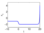
The sketch of the phase portrait, Figure 6, is an accurate representation of the full system that does not change over the time considered, since this continuation is for $t_{0}=-10$ and $T_{\mathrm{end}}=-9$ and hence $\lambda\approx 0$. The phase portrait contains two saddles, which are located close to the equilibrium points of $S_{-}$ and $U_{-}$ and one center close to the origin. The saddles are offset to the left of $S_{-}$ and $U_{-}$ by approximately $D/2$. The center of the elliptic region is located at $(x_{1},x_{2})\approx(D,0)$.

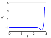
The initial trajectory after step 1 ($x_{T}=x_{0}=-1$) is a unique solution that is contained within the elliptic region near the saddle (see blue trajectory Figure 6). The boundary condition $x_{1}(t_{0})=x_{0}$ ensures that all trajectories start on the dashed line $S_{-}=-1$. During continuation in $x_{T}$ the trajectories need to travel further but still in the same time interval ($t_{0}=-10$, $T_{\mathrm{end}}=-9$) as $x_{T}$ is increased. Therefore, the starting position increases in the $x_{2}$ direction where the vector field has a larger $x_{1}$ component. This enables the trajectories to travel faster in order to travel further in the same time period. See Figure 6 for intermediate phase portraits in this continuation, Figure 14(a) for the phase portrait and 14(b) for the time profile of the (final) trajectory with $x_{T}=4$.

(a) $x_{T}=4$

(b) Optimal path after $x_{T}$ continuation step.

Figure 14: (a) Trajectory in $(x_{1},x_{2})$ - plane, (b) optimal path after $x_{T}$ continuation. $t_{0}=-10$, $\epsilon=1.25$, $D=0.05$.

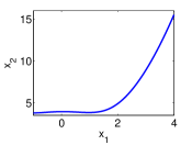
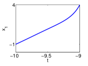
This trajectory corresponds to the optimal path for a purely noise-induced tipping since $\lambda$ is close to stationary. One would expect the optimal time for tipping to be a result of both noise and rate-induced tipping.

C.3 Step 3: $T_{\mathrm{end}}$ continuation

The next step is to perform a continuation in $T_{\mathrm{end}}$ while monitoring $m$ for roots (or $M$ for critical points). Since $M$ may have several local minima and maxima for increasing $T_{\mathrm{end}}$we continue in $T_{\mathrm{end}}$ too sufficiently large values where we observe the asymptotic monotone decrease of $M$. In our example, we continued $T_{\mathrm{end}}$ from $-9$ to $20$, monitoring the bifurcation diagram in the $(T_{\mathrm{end}},M)$ - plane (not shown but similar to Figure 5(b)).

For choice of parameter values displayed in Figure 5(b) there is only one critical point of $M$, which corresponds to the maximum we are interested in. Figure 15(a) displays the optimal path after the $T_{\mathrm{end}}$ continuation step, for $T_{\mathrm{end}}=20$. For $T_{\mathrm{end}}=20$ the optimal path reaches the saddle at $t\approx 1$, but waits at the saddle until $t\approx 18$ before escaping to $x_{T}$, which is optimal only in the limit $D\to 0$. Therefore, we detect when $m=0$ which satisfies the integral condition (26) to identify the maximum of $M$ and hence achieve the optimal path in an optimal time, see Figure 15(b).

(a) $T_{\mathrm{end}}=20$.

(b) $T_{\mathrm{end}}\approx 1.43$.

Figure 15: Comparison between optimal paths for $T_{\mathrm{end}}=20$ and after $m$ continuation is completed. $t_{0}=-10$, $\epsilon=1.25$, $D=0.05$

References

- Wieczorek et al. (2011) S. Wieczorek, P. Ashwin, C. M. Luke, and P. M. Cox, “Excitability in ramped systems: the compost-bomb instability,” in Proceedings of the Royal Society of London A: Mathematical, Physical and Engineering Sciences, Vol. 467 (The Royal Society, 2011) pp. 1243–1269.
- Boulton, Allison, and Lenton (2014) C. A. Boulton, L. C. Allison, and T. M. Lenton, “Early warning signals of Atlantic Meridional Overturning Circulation collapse in a fully coupled climate model,” Nature Communications 5 (2014).
- Xu et al. (2015) C. Xu, E. H. Van Nes, M. Holmgren, S. Kéfi, and M. Scheffer, “Local facilitation may cause tipping points on a landscape level preceded by early-warning indicators,” The American Naturalist 186, E000–E000 (2015).
- Ashwin, Perryman, and Wieczorek (2015) P. Ashwin, C. Perryman, and S. Wieczorek, “Parameter shifts for nonautonomous systems in low dimension: Bifurcation-and rate-induced tipping,” arXiv preprint arXiv:1506.07734 (2015).
- Lenton (2011) T. M. Lenton, “Early warning of climate tipping points,” Nature Climate Change 1, 201–209 (2011).
- Williamson and Lenton (2015) M. S. Williamson and T. M. Lenton, “Detection of bifurcations in noisy coupled systems from multiple time series,” Chaos: An Interdisciplinary Journal of Nonlinear Science 25, 036407 (2015).
- Holland, Bitz, and Tremblay (2006) M. M. Holland, C. M. Bitz, and B. Tremblay, “Future abrupt reductions in the summer Arctic sea ice,” Geophysical Research Letters 33 (2006).
- Held and Kleinen (2004) H. Held and T. Kleinen, “Detection of climate system bifurcations by degenerate fingerprinting,” Geophysical Research Letters 31 (2004).
- Malhi et al. (2009) Y. Malhi, L. E. Aragão, D. Galbraith, C. Huntingford, R. Fisher, P. Zelazowski, S. Sitch, C. McSweeney, and P. Meir, “Exploring the likelihood and mechanism of a climate-change-induced dieback of the Amazon rainforest,” Proceedings of the National Academy of Sciences 106, 20610–20615 (2009).
- Laurance et al. (2011) W. F. Laurance, B. Dell, S. M. Turton, M. J. Lawes, L. B. Hutley, H. McCallum, P. Dale, M. Bird, G. Hardy, G. Prideaux, et al., “The 10 Australian ecosystems most vulnerable to tipping points,” Biological Conservation 144, 1472–1480 (2011).
- Clark et al. (2013) G. F. Clark, J. S. Stark, E. L. Johnston, J. W. Runcie, P. M. Goldsworthy, B. Raymond, and M. J. Riddle, “Light-driven tipping points in polar ecosystems,” Global Change Biology 19, 3749–3761 (2013).
- Hoegh-Guldberg et al. (2007) O. Hoegh-Guldberg, P. Mumby, A. Hooten, R. Steneck, P. Greenfield, E. Gomez, C. Harvell, P. Sale, A. Edwards, K. Caldeira, et al., “Coral reefs under rapid climate change and ocean acidification,” Science 318, 1737–1742 (2007).
- Yan, Woodard, and Sornette (2010) W. Yan, R. Woodard, and D. Sornette, “Diagnosis and prediction of tipping points in financial markets: Crashes and rebounds,” Physics Procedia 3, 1641–1657 (2010).
- Lenton et al. (2008) T. M. Lenton, H. Held, E. Kriegler, J. W. Hall, W. Lucht, S. Rahmstorf, and H. J. Schellnhuber, “Tipping elements in the Earth’s climate system,” Proceedings of the National Academy of Sciences 105, 1786–1793 (2008).
- Ashwin et al. (2012) P. Ashwin, S. Wieczorek, R. Vitolo, and P. Cox, “Tipping points in open systems: bifurcation, noise-induced and rate-dependent examples in the climate system,” Philosophical Transactions of the Royal Society of London A: Mathematical, Physical and Engineering Sciences 370, 1166–1184 (2012), Correction co-authored with C. Perryman (Née Hobbs) 371, 20130098 (2013).
- Scheffer et al. (2009) M. Scheffer, J. Bascompte, W. A. Brock, V. Brovkin, S. R. Carpenter, V. Dakos, H. Held, E. H. Van Nes, M. Rietkerk, and G. Sugihara, “Early-warning signals for critical transitions,” Nature 461, 53–59 (2009).
- Scheffer et al. (2012) M. Scheffer, S. R. Carpenter, T. M. Lenton, J. Bascompte, W. Brock, V. Dakos, J. Van De Koppel, I. A. Van De Leemput, S. A. Levin, E. H. Van Nes, et al., “Anticipating critical transitions,” science 338, 344–348 (2012).
- Kuehn (2015) C. Kuehn, Multiple Time Scale Dynamics (Springer, 2015).
- Ditlevsen and Johnsen (2010) P. D. Ditlevsen and S. J. Johnsen, “Tipping points: early warning and wishful thinking,” Geophysical Research Letters 37 (2010).
- Wang et al. (2012) R. Wang, J. A. Dearing, P. G. Langdon, E. Zhang, X. Yang, V. Dakos, and M. Scheffer, “Flickering gives early warning signals of a critical transition to a eutrophic lake state,” Nature 492, 419–422 (2012).
- Dakos et al. (2008) V. Dakos, M. Scheffer, E. H. van Nes, V. Brovkin, V. Petoukhov, and H. Held, “Slowing down as an early warning signal for abrupt climate change,” Proceedings of the National Academy of Sciences 105, 14308–14312 (2008).
- Luke and Cox (2011) C. Luke and P. Cox, “Soil carbon and climate change: from the Jenkinson effect to the compost-bomb instability,” European Journal of Soil Science 62, 5–12 (2011).
- Stocker and Schmittner (1997) T. F. Stocker and A. Schmittner, “Influence of CO2 emission rates on the stability of the thermohaline circulation,” Nature 388, 862–865 (1997).
- Scheffer et al. (2008) M. Scheffer, E. H. Van Nes, M. Holmgren, and T. Hughes, “Pulse-driven loss of top-down control: the critical-rate hypothesis,” Ecosystems 11, 226–237 (2008).
- Perryman and Wieczorek (2014) C. Perryman and S. Wieczorek, “Adapting to a changing environment: non-obvious thresholds in multi-scale systems,” Proceedings of the Royal Society A: Mathematical, Physical and Engineering Science 470, 20140226 (2014).
- Perryman and Wieczorek (2015) C. Perryman and S. Wieczorek, “How fast is too fast? rate-induced bifurcations in multiple time-scale systems,” PhD thesis: In preparation (2015).
- Aalen, Borgan, and Gjessing (2008) O. Aalen, O. Borgan, and H. Gjessing, Survival and event history analysis: a process point of view (Springer Science & Business Media, 2008).
- Berglund and Gentz (2004) N. Berglund and B. Gentz, “On the noise-induced passage through an unstable periodic orbit i: Two-level model,” Journal of statistical physics 114, 1577–1618 (2004).
- Zhang (2008) B. W. Zhang, Theory and Simulation of Rare Events in Stochastic Systems (ProQuest, 2008).
- Lin and Ho (2011) W.-T. Lin and C.-L. Ho, “Similarity solutions of a class of perturbative Fokker-Planck equation,” Journal of Mathematical Physics 52, 073701 (2011).
- Ho and Dai (2008) C.-L. Ho and Y.-M. Dai, “A perturbative approach to a class of Fokker–Planck equations,” Modern Physics Letters B 22, 475–481 (2008).
- Ren, Vanden-Eijnden et al. (2004) W. Ren, E. Vanden-Eijnden, et al., “Minimum action method for the study of rare events,” Communications on Pure and Applied Mathematics 57, 637–656 (2004).
- Doedel (2007) E. J. Doedel, “Lecture notes on numerical analysis of nonlinear equations,” in Numerical Continuation Methods for Dynamical Systems: Path following and boundary value problems, edited by B. Krauskopf, H. M. Osinga, and J. Galán-Vioque (Springer-Verlag, Dordrecht, 2007) pp. 1–49.
- Oldeman, Doedel, and Paffenroth (2013) B. Oldeman, E. Doedel, and R. Paffenroth, “Auto-07p: http://sourceforge.net/projects/auto-07p/,” (2013).
- Chaichian and Demichev (2001) M. Chaichian and A. Demichev, Path Integrals in Physics: Volume I Stochastic Processes and Quantum Mechanics (Institute of Physics, 2001).
- Bakhtin (2013) Y. Bakhtin, “Gumbel distribution in exit problems,” arXiv preprint arXiv:1307.7060 (2013).