Transit timing to first order in eccentricity

Abstract

Characterization of transiting planets with transit timing variations (TTVs) requires understanding how to translate the observed TTVs into masses and orbital elements of the planets. This can be challenging in multi-planet transiting systems, but fortunately these systems tend to be nearly plane-parallel and low eccentricity. Here we present a novel derivation of analytic formulae for TTVs that are accurate to first order in the planet-star mass ratios and in the orbital eccentricities. These formulae are accurate in proximity to first order resonances, as well as away from resonance, and compare well with more computationally expensive N-body integrations in the low eccentricity, low mass-ratio regime when applied to simulated and to actual multi-transiting Kepler planet systems. We make code available for implementing these formulae.

1. Introduction

No planet orbits on a precisely Keplerian orbit: post-Newtonian corrections, stellar oblateness, and, most importantly, planetary perturbations cause deviations from a periodic ephemeris for transiting exoplanets (Miralda-Escudé, 2002; Schneider, 2003, 2004; Holman & Murray, 2005; Agol et al., 2005; Heyl & Gladman, 2007; Nesvorný & Morbidelli, 2008; Fabrycky, 2010). Transit-timing variations (TTVs) have been used to confirm that transit signals are in fact due to planets (Holman et al., 2010; Ford et al., 2012b; Steffen et al., 2012, 2013; Fabrycky et al., 2012; Ford et al., 2012a; Xie, 2013; Xie et al., 2014), to detect and characterize non-transiting planets (Ballard et al., 2011; Nesvorný et al., 2012, 2013), and to make precise measurements of the masses and dynamical states of multi-transiting exoplanet systems (e.g. Carter et al., 2012).

For the latter two applications, fast computation of TTVs is required for rapid searching through parameter space for perturbing companions, and for rapid computation of the posterior distributions of the masses and orbital elements of transiting planet systems. Numerical computation of TTVs can be sped up through symplectic integration, through a more efficient numerical solution of Kepler’s equation, and through transit time interpolation (Deck et al., 2014); however, this approach can still be too computationally intensive for high multiplicity systems, and does not pinpoint the physical origin of constraints upon planetary system properties. Analytic formulae based on perturbation theory can greatly speed computation, but the perturbation theory to high order in eccentricity and inclination becomes complicated quickly, and numerical codes that implement the analytic formulae have not been released or widely used (Nesvorný & Morbidelli, 2008; Nesvorný, 2009; Nesvorný & Beaugé, 2010). Much can be accomplished with first order (in eccentricity) perturbation theory because orbital eccentricities of many planets exhibiting TTVs are small. TTVs are most easily observed for pairs of planets near a mean motion resonance; thanks to the low eccentricity of the systems in consideration (Fabrycky et al., 2014; Hadden & Lithwick, 2014; Limbach & Turner, 2014; Van Eylen & Albrecht, 2015), the first order resonances are most represented among TTV pairs, and it is for first order resonances that a first order theory is adequate. TTVs caused by these first order resonant interactions are primarily sinusoidal and are subject to a degeneracy between mass and eccentricity (Boué et al., 2012), caused by mixing of two frequencies of perturbation which are aliased at the frequency of the transiting planet, as explained in an elegant analysis by Lithwick et al. (2012, hereafter LXW12). To break this degeneracy requires the measurement of additional modes, such as the short-timescale TTVs known as ‘chopping’ variations (Holman et al., 2010; Deck & Agol, 2015), or statistical analysis of many systems (Wu & Lithwick, 2013; Hadden & Lithwick, 2014; Xie, 2014). In addition, the LXW12 analysis is only approximate, and breaks down for pairs further from resonance (Deck & Agol, 2015). These issues motivate the current paper in which we derive an explicit formula for TTVs accurate to first order in eccentricity and planet-star mass ratio, valid for (nearly) plane-parallel transiting planets (although Nesvorný & Vokrouhlický 2014 showed that mutual inclinations of planets can be large and still be well described by coplanar TTVs).

We expect that these results will be useful a) for determining how different frequencies within the TTV signal constrain the planetary masses and orbital elements (Deck & Agol, 2015); b) for analyzing systems with a large number of interacting transiting planets by making linear additions of the analytic formula for pairs of planets (Lissauer et al., 2013; Jontof-Hutter et al., 2014); and c) for rapid search through parameter space of perturbing planets.

We first summarize the TTV solution to first order in eccentricity and mass in §2 (the full derivation is given in appendix A new approach to TTVs). We then compare these with prior results, both analytic and numeric (§3), including comparison of analytic and numeric analyses of specific systems. We discuss the numerical implementation and speed in §4. We end with a discussion of the possible applications and future directions (§5).

2. First-order solution:

Here we give a complete summary of the assumptions and variables used, and the solution to the first-order equations for readers that wish to simply use the results of this computation. The details of the derivation are given in Appendix A new approach to TTVs. Since multi-planet transiting systems typically have nearly edge-on orbits and hence small mutual inclinations, it is usually sufficient in analytic approximations to treat the problem in the plane-parallel approximation. This leaves four orbital elements for each planet (semi-major axis, $a_{i}$, mean longitude, $\lambda_{i}$, eccentricity, $e_{i}$, and longitude of periastron, $\varpi_{i}$), plus the mass ratio of each planet to the star, $m_{1}/m_{\star},m_{2}/m_{\star}$, where $m_{1}$ is the mass of the inner planet, $m_{2}$ is the mass of the outer planet, and $m_{\star}$ is the mass of the star. For nearly circular planetary orbits, there are two small dimensionless parameters in the problem: $\mu_{i}=m_{i}/m_{\star}$ and $e_{i}$. The usual procedure for computing transit timing variations is to: 1) to write down a Hamiltonian (or disturbing function) for perturbations due to another planet; 2) expand the Hamiltonian as a function of the orbital elements to the order in eccentricity desired plus one (e.g. if a transit timing solution is needed to first order in eccentricity, then the Hamiltonian must be expanded to second order in eccentricity), including the linear combinations of mean-longitudes leading to the important resonant terms necessary for sufficient accuracy; 3) compute the variation in the orbital elements using Hamilton’s equations, which are four first-order partial differential equations for each planet, and involves differentiating the Hamiltonian with respect to the orbital elements (which can be a rather complex operation); 4) integrate the resulting equations as a function of time; 5) compute the true longitudes, $\theta_{i}=\theta_{i,K}+\delta\theta_{i}$, as a function of time, where $\theta_{i,K}$ is the unperturbed Keplerian orbit, and $\delta\theta_{i}$ is the perturbation of the $i$th planet caused by its planet companion(s); 6) compute the transit timing variations:

$$\delta t_{i}=-\dot{\theta}_{i,K}^{-1}\delta\theta_{i}.$$ (1)

This is the approach taken by Agol et al. (2005), Nesvorný & Vokrouhlický (2014), and LXW12. A different approach employing Hamiltonian perturbation theory (Nesvorný & Morbidelli, 2008) was used in Deck & Agol (2015). This involves determining the canonical transformation between the full canonical orbital element set and the average set; the TTVs, which are deviations from an average “Keplerian” orbit, can be derived from this transformation.

The standard procedure outlined in detail above (based on Hamilton’s equations) has the advantages of requiring only first-order differential equations for the computation, and the advantage of using standard methods in celestial mechanics for the computation. However, there are two possible drawbacks: 1) the expansion of the Hamiltonian in orbital elements can be rather complex; 2) the main quantity of interest for transit-timing variations is $\delta\theta_{i}$, rather than the perturbed orbital elements. The derivation based on canonical transformations (Nesvorný & Morbidelli, 2008), though elegant, has the disadvantage of requiring the extra machinery and knowledge of Hamiltonian perturbation theory.

In our new derivation we forgo computing the orbital elements, and simply treat the problem in polar coordinates $(r_{i},\theta_{i})$. We then use Newton’s equations in terms of a disturbing function which can be expressed as a function of polar coordinates, with the added advantage that Newton’s equations make clearer which forces are causing the perturbations. This approach has some possible advantages: 1) only two differential equations are necessary (albeit second-order rather than first-order); 2) the derivatives of the disturbing function with respect to the polar coordinates are easy to compute; 3) the perturbed polar coordinates directly yield the transit timing variations; 4) the resulting expression is more compact than in the Hamiltonian formulation. The second-order differential equation may seem like a drawback, but it can be solved using complex notation (as in LXW12) and by expanding the derivatives of the disturbing function in terms of orbital elements, which yields harmonic functions which are easy to integrate. The final answer is expressed as a sum over harmonics of the perturbing planet’s orbital frequency (Deck & Agol, 2015). Each coefficient for each planet in the harmonic series solution can be solved for by inverting three two-by-two matrices, which have a standard format, resulting directly in the transit timing variations at a particular frequency.

The unperturbed orbital frequencies, $n_{i}=2\pi/P_{i}$, are defined by $n_{i}^{2}=Gm_{\star}/a_{i}^{3}$. As usual, $\alpha=a_{1}/a_{2}\approx(P_{1}/P_{2})^{2/3}$. We define $\tilde{A}_{jmn}=a_{1}^{m}a_{2}^{n+1}\frac{\partial^{m+n}}{\partial a_{1}^{m}\partial a_{2}^{n}}\left(a_{2}^{-1}b_{1/2}^{(j)}(\alpha)\right)$ where $b_{1/2}^{(j)}(\alpha)$ is the Laplace coefficient,

$$b_{1/2}^{(j)}(\alpha)=\frac{1}{\pi}\int_{0}^{2\pi}d\theta\frac{\cos{(j\theta)}}{(1+\alpha^{2}-2\alpha\cos{\theta})^{1/2}}.$$ (2)

The difference in mean longitude of the planets is $\psi=\lambda_{1}-\lambda_{2}$. Auxiliary dimensionless quantities are:

$$\beta_{j} =j(n_{1}-n_{2})/n_{1}=j(1-\alpha^{3/2}),$$ (3)

$$\kappa_{j} =j(n_{1}-n_{2})/n_{2}=j(\alpha^{-3/2}-1).$$ (4)

The functions $\tilde{A}_{jmn}$ we use below are given by:

$$\tilde{A}_{j00} = b_{1/2}^{(j)}(\alpha),$$ (5)

$$\tilde{A}_{j10} = \alpha\partial b_{1/2}^{(j)}/\partial\alpha,$$ (6)

$$\tilde{A}_{j20} = \alpha^{2}\partial^{2}b_{1/2}^{(j)}/\partial\alpha^{2},$$ (7)

$$\tilde{A}_{j01} = -(\tilde{A}_{j10}+\tilde{A}_{j00})=-(\alpha\partial b_{1/2}^{(j)}/\partial\alpha+b_{1/2}^{(j)}),$$ (8)

$$\tilde{A}_{j02} = 2\tilde{A}_{j00}+4\tilde{A}_{j10}+\tilde{A}_{j20}=2b_{1/2}^{(j)}+4\alpha\partial b_{1/2}^{(j)}/\partial\alpha+\alpha^{2}\partial^{2}b_{1/2}^{(j)}/\partial\alpha^{2},$$ (9)

$$\tilde{A}_{j11} = -(2\tilde{A}_{j10}+\tilde{A}_{j20})=-2\alpha\partial b_{1/2}^{(j)}/\partial\alpha-\alpha^{2}\partial^{2}b_{1/2}^{(j)}/\partial\alpha^{2}.$$ (10)

To use this solution in computing TTVs, the longitudes need to be computed from the observed transit times; the mean ephemeris, $(t_{0,i},P_{i})$, may be used in computing the (unperturbed) orbital ephemeris. Now, the mean longitudes are given to first order in eccentricity by

$$\lambda_{i}=2\pi\left(\frac{t-t_{0,i}}{P_{i}}\right)+2e_{i}\sin{\varpi_{i}},$$ (11)

if we assume that the orbital reference is along the line of sight, and thus $\lambda_{i}\approx 0$ at the times of transit.

The solutions for the inner planet ($i=1$) and outer planet ($i=2$) are given by:

$$\delta t_{1} = \frac{P_{1}}{2\pi}\mu_{2}\sum_{j\geq 1}\Big{[}f_{1,j}^{(0)}\sin{(j\psi)}+f_{1,j}^{(-1)}e_{1}\sin{\left[j\psi-(\lambda_{1}-\varpi_{1})\right]}+f_{1,j}^{(+1)}e_{1}\sin{\left[j\psi+(\lambda_{1}-\varpi_{1})\right]}$$ (12)

$$+ f_{1,j-1}^{(-2)}e_{2}\sin{\left[j\psi-(\lambda_{1}-\varpi_{2})\right]}+f_{1,j+1}^{(+2)}e_{2}\sin{\left[j\psi+(\lambda_{1}-\varpi_{2})\right]}\Big{]},$$ (13)

$$\delta t_{2} = \frac{P_{2}}{2\pi}\mu_{1}\sum_{j\geq 1}\Big{[}f_{2,j}^{(0)}\sin{(j\psi)}+f_{2,j}^{(-2)}e_{2}\sin{\left[j\psi-(\lambda_{2}-\varpi_{2})\right]}+f_{2,j}^{(+2)}e_{2}\sin{\left[j\psi+(\lambda_{2}-\varpi_{2})\right]}$$ (14)

$$+ f_{2,j+1}^{(-1)}e_{1}\sin{\left[j\psi-(\lambda_{2}-\varpi_{1})\right]}+f_{2,j-1}^{(+1)}e_{1}\sin{\left[j\psi+(\lambda_{2}-\varpi_{1})\right]}\Big{]},$$ (15)

where the functions $f_{i,j}^{(\pm k)}$ are given by:

$$f_{i,j}^{(\pm k)}(\alpha) = u(\gamma,c_{1},c_{2})+\delta_{ik}v_{\pm}(\zeta,d_{1},d_{2}),$$ (16)

$$u(\gamma,c_{1},c_{2}) = \frac{\left(3+\gamma^{2}\right)c_{1}+2\gamma c_{2}}{\gamma^{2}\left(1-\gamma^{2}\right)}$$ (17)

$$v_{\pm}(\zeta,d_{1},d_{2}) = \frac{\left(\pm\left(1-\zeta^{2}\right)+6\zeta\right)d_{1}+\left(2+\zeta^{2}\right)d_{2}}{\zeta(1-\zeta^{2})(\zeta\pm 1)(\zeta\pm 2)}.$$ (18)

where $\gamma$, $c_{1}$, and $c_{2}$ and $\zeta$, $d_{1}$, and $d_{2}$ are given in Table 1, and $\delta_{ik}$ is the Kronecker delta function. Note that the top signs in $\pm,\mp$ correspond to $+k$ values, while the bottom correspond to $-k$. The functions $f_{i,j}^{(\pm k)}$ are solely a function of $j$, $\pm k$, and $\alpha$.

Table 1Coefficients for $u(\gamma,c_{1},c_{2})$ and $v_{\pm}(\zeta,d_{1},d_{2})$ in first-order TTV solution (the $v_{\pm}$ coefficients correspond to the $k$ values in brackets [..]).

$i$	$\pm k$	$\gamma[\zeta]$	$c_{1}[d_{1}]$	$c_{2}[d_{2}]$
1	$0[\pm 1]$	$\beta_{j}$	$\alpha j\left(\tilde{A}_{j00}-\alpha\delta_{j1}\right)$	$\alpha\left(\tilde{A}_{j10}-\alpha\delta_{j1}\right)$
1	$\pm$1	$\beta_{j}\pm 1$	$\alpha j\left(\pm j\tilde{A}_{j00}-\frac{1}{2}\tilde{A}_{j10}+\frac{1}{2}(1\mp 2)\alpha\delta_{j1}\right)$	$\alpha\left(\pm j\tilde{A}_{j10}-\frac{1}{2}\tilde{A}_{j20}\mp\alpha\delta_{j1}\right)$
1	$\pm$2	$\beta_{j}\pm\alpha^{3/2}$	$\alpha j\left(\mp j\tilde{A}_{j00}-\frac{1}{2}\tilde{A}_{j01}-(1\mp 1)\alpha\delta_{j1}\right)$	$\alpha\left(\mp j\tilde{A}_{j10}-\frac{1}{2}\tilde{A}_{j11}-(1\mp 1)\alpha\delta_{j1}\right)$
2	$0[\pm 2]$	$\kappa_{j}$	$-j\left(\tilde{A}_{j00}-\alpha^{-2}\delta_{j1}\right)$	$\tilde{A}_{j01}-\alpha^{-2}\delta_{j1}$
2	$\pm 1$	$\kappa_{j}\pm\alpha^{-3/2}$	$-j\left(\pm j\tilde{A}_{j00}-\frac{1}{2}\tilde{A}_{j10}-(1\pm 1)\alpha^{-2}\delta_{j1}\right)$	$\pm j\tilde{A}_{j01}-\frac{1}{2}\tilde{A}_{j11}-(1\pm 1)\alpha^{-2}\delta_{j1}$
2	$\pm 2$	$\kappa_{j}\pm 1$	$-j\left(\mp j\tilde{A}_{j00}-\frac{1}{2}\tilde{A}_{j01}+\frac{1}{2}(1\pm 2)\alpha^{-2}\delta_{j1}\right)$	$\mp j\tilde{A}_{j01}-\frac{1}{2}\tilde{A}_{j02}\pm\alpha^{-2}\delta_{j1}$

In practice the sum over $j$ from 1 to $\infty$ must be truncated at a finite value of $j_{max}$. Typically $j_{max}$ does not need to be chosen to be too large since the Laplace coefficients decline in amplitude with $j$ (Deck & Agol, 2015). We recommend choosing a $j_{max}$ large enough such that the resulting computation is converged.

As an example of using Table 1, the coefficient $f_{1,j}^{(-1)}$ has $i=k=1$, $\gamma=\beta_{j}-1$, $c_{1}=\alpha j\left(-j\tilde{A}_{j00}-\frac{1}{2}\tilde{A}_{j10}+\frac{3}{2}\alpha\delta_{j1}\right)$ and $c_{2}=\alpha\left(-j\tilde{A}_{j10}-\frac{1}{2}\tilde{A}_{j20}+\alpha\delta_{j1}\right)$, $\zeta=\beta_{j}$, $d_{1}=\alpha j\left(\tilde{A}_{j00}-\alpha\delta_{j1}\right)$, and $d_{2}=\alpha\left(\tilde{A}_{j10}-\alpha\delta_{j1}\right)$. Then, the coefficient is given by:

$$f_{1,j}^{(-1)}(\alpha)=u(\beta_{j}-1,c_{1},c_{2})+v_{-}(\beta_{j},d_{1},d_{2}).$$ (19)

3. Comparison with other formulae

The zeroth-order solution (in the limit $e_{1}=e_{2}=0$) compares exactly with the results given in Agol et al. (2005), Nesvorný & Vokrouhlický (2014), and Deck & Agol (2015) which were derived with Hamilton’s equations and the approach based on canonical transformations; this is reassuring given the very different approach used in this derivation. We have also rederived the first-order eccentricity equations using the approach based on canonical perturbation theory employed in Deck & Agol (2015), and found exact agreement with the results presented here to first order in eccentricity.

In Figures (1) and (2) we plot the eccentricity-dependent coefficients, $f_{i,j}^{(\pm k)}(\alpha)$, as a function of period ratio, $P_{2}/P_{1}\approx\alpha^{-3/2}$. The zeroth-order eccentricity coefficients are plotted in Deck & Agol (2015). The first-order coefficients can show three singularities for the terms with superscripts $(-1)$ and $(-2)$ near first-order resonance, second-order resonance, and $\alpha=1$.

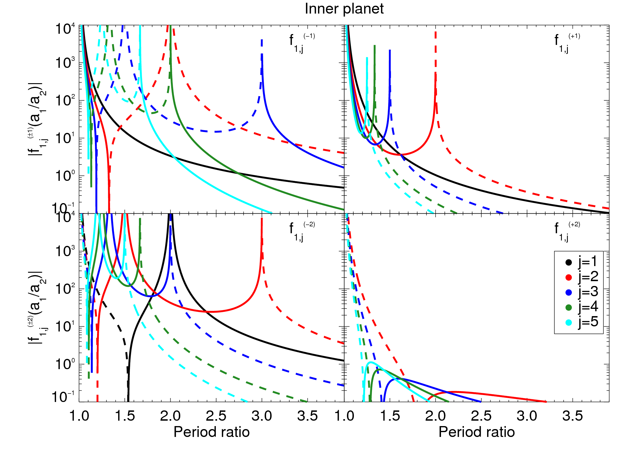
Figure 1.— Dimensionless coefficients, $f_{1,j}^{(\pm k)}$ for the inner planet. The dashed lines show where the coefficients are negative.

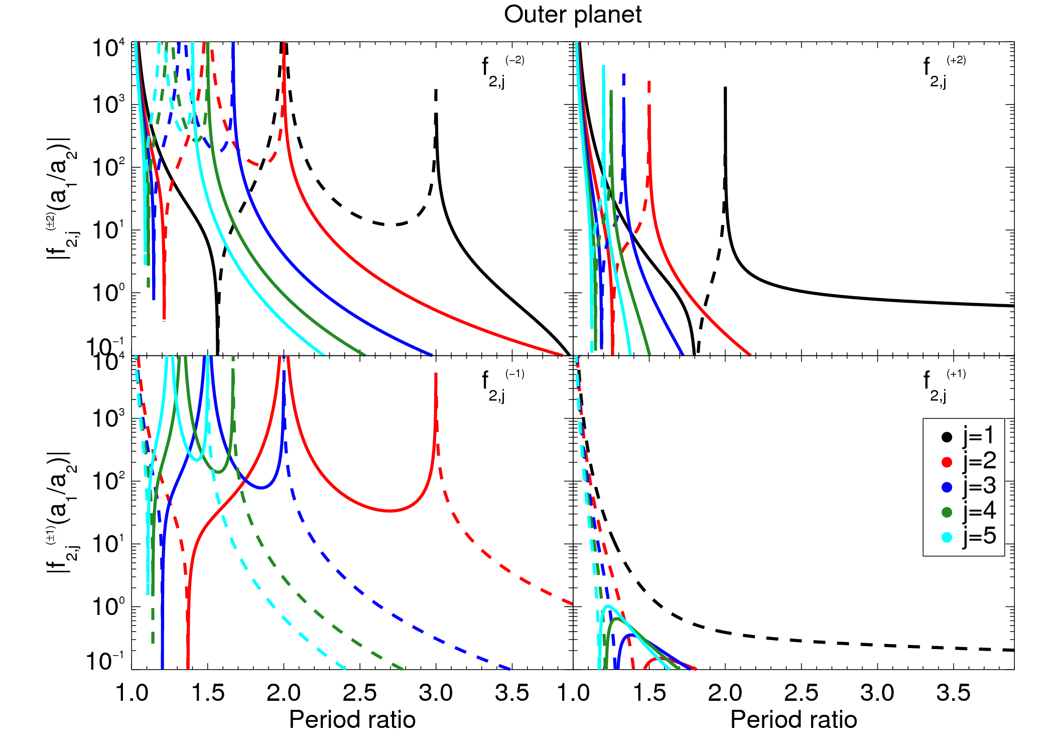
Figure 2.— Dimensionless coefficients, $f_{2,j}^{(\pm k)}$ for the outer planet. The dashed lines show where the coefficients are negative.

3.1. Comparison with first order resonant equations

LXW12 present a formula valid near (but not in) first order mean-motion resonances that captures the behavior of resonant terms in an elegant, but approximate, manner. Here we compare the complete formulae given here to their near-resonant formulae.

The expressions for $u$ and $v_{\pm}$ do not show the same dependence in the denominator as the expressions in LXW12; their expression just contains the resonant frequency, $jn_{1}-(j+1)n_{2}$, while ours contains additional frequencies. We carried out the partial fraction expansion of $u$ to isolate the denominator which matches LXW12’s expression, and we find that the expressions agree exactly with their expressions (A28) and (A29).

To compare our full expression with LXW12’s, we have computed the eccentricity-dependent $j=2$ (near 2:3) expression for the inner and outer planets (as this term is unaffected by the indirect terms). We re-write the TTV formulae derived here and in LXW12 for the $i-$th planet perturbed by planet $k$ as

$$\delta t_{i} =\frac{\mu_{k}}{n_{i}}\sum_{j\geq 1}\bigg{[}A_{i,i}^{j}e_{i}\sin{(j\lambda_{k}+\phi_{i,i}^{j})}+A_{i,k}^{j}e_{k}\sin{(j\lambda_{k}+\phi_{i,k}^{j})}\bigg{]}$$ (20)

where we have set $\theta_{i}=\lambda_{i}=0$ at transit (this incurs some error, at order $e$, but that is a second order effect since we are comparing the TTV term linear in $e$). When written in this way, the amplitude and phase depend only on $\alpha,\varpi_{1}$, and $\varpi_{2}$.

For the 3:2 resonance, the LXW12 resonant term depends on $e_{1}/(2n_{1}-3n_{2})^{2}$ and $e_{2}/(2n_{1}-3n_{2})^{2}$, which both decline quickly away from resonance, and thus other terms that depend on $e_{1}$ and $e_{2}$ make a more significant contribution further from resonance; hence our formulae agree close to resonance but diverge away from exact commensurability. Figure 3 shows the fractional error in the amplitude $A$ and phase $\phi$ of the terms that are proportional to the eccentricities of the planets for $\varpi_{1}\approx\varpi_{2}=0.45$ radians. The error in the LXW12 expression (A28) and (A29) reaches $\approx$20% at a 5% separation from exact resonance in this case; if we use the further approximate expression given in their main paper in lieu of (A28), the discrepancy for the inner planet increases to $\approx$30%. This is similar to the error in the zeroth-order component of their expression (Deck & Agol, 2015). The zeroth- and first-order eccentricity terms have a different dependence on longitudes: for example, for the inner planet the zeroth order term scales as $e^{\mathbbm{i}(j+1)(\lambda_{1}-\lambda_{2})}$, while the first order term scales as $e^{\mathbbm{i}(j\lambda_{1}-(j+1)\lambda_{2})}$, where $\mathbbm{i}=\sqrt{-1}$. Since the mean longitude of the inner planet is nearly identical at each transit of the inner planet, the $\lambda_{1}$ term in the exponent is approximately constant, while the $\lambda_{2}$ dependence is identical in both terms, leading to aliasing of these coefficients. Thus the error incurred in their approximation can lead to a different phase dependence and amplitude for this aliased term away from resonance.

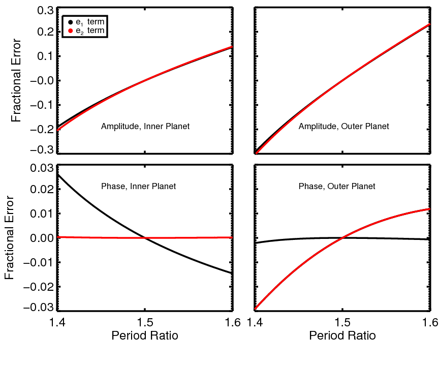
Figure 3.— Fractional error in the coefficients of the 3:2 resonant TTV expression given in LXW12 compared with the $j=2$ terms of our analytic expression. Black indicates dependence on the $e_{1}$ term, while red indicates the dependence on the $e_{2}$ term. The top show the fractional errors in the amplitudes of the inner (left) and outer (right) planets. The bottom shows the fractional error on the phases.

3.2. Comparison with N-body integrations

We have carried out extensive integrations of three-body systems using TTVFast (Deck et al., 2014), and compared the results with the first-order analytic formulae (equation 12). Note that the TTVFast code uses the convention of the longitude of periastron being measured from the sky plane to match the convention of radial velocity surveys, while here we use the observer’s line of sight as the reference direction, as done in LXW12 and Deck & Agol (2015). The longitudes computed from the TTVFast code need to have $\pi/2$ subtracted to make the plots shown below. In addition, the orbital elements accepted by TTVFast are the instantaneous/osculating orbital elements (initial conditions) at the specified initial time, while the orbital elements used in these formulae are the mean orbital elements of the planets over the timescale of the observations.

3.2.1 Eccentricity and period ratio dependence

Figure 4 compares the precision of the analytic formula as a function of $\alpha=(P_{1}/P_{2})^{2/3}$ and eccentricity of both planets, which are set to be equal, $e_{1}=e_{2}$. We have set $\varpi_{1}=\varpi_{2}+\pi$, which we found (approximately) maximizes the discrepancy of the analytic model compared with the N-body model, and $\varpi_{1}=\varpi_{2}$ which (approximately) minimizes the discrepancy; hence the figures bracket the precision of the analytic model. This is due to the fact that the anti-aligned longitude geometry causes the planets to be closer at conjunctions that occur when the inner planet is at apoapse and the outer is at periapse; their proximity at these conjunctions causes their gravitational interactions to be more sensitive to deviations from the epicyclic approximation, which are second order in eccentricity, and thus missing from our computation. We have assumed that the period of the inner planet is $P_{1}=30$ days, and we have integrated the system with TTVFast for 1600 days, about the duration of the initial Kepler mission, assuming plane-parallel orbits. For these tests we assume $\mu_{1}=\mu_{2}=10^{-5}$, and we selected random values for the longitudes of the planets at the initial time. For each set of initial conditions, we output the orbital elements at regular intervals during the N-body integration, from which we computed the average orbital elements over the duration of the integration. These averaged orbital elements were used for computing the amplitudes of the analytic model, which we summed up to $j_{max}=10$. We optimized the fit of the analytic formula to the numerical TTVs by allowing the ephemerides of the planets to vary in the formula, but holding the eccentricity vectors and mass ratios fixed at the values computed from the time-averaged N-body simulation, while we computed $\alpha$ in the analytic formula from the ratio of the periods derived from the best-fit ephemerides.

The fractional precision was computed from the RMS of the residuals of the best analytic model fit to the TTVs, divided by the RMS of the TTVs computed from the N-body integration. Figure 4 shows that the formula works to better than 10% precision for a wide range of $\alpha-e$ parameter space. However, it fails near resonances, most significantly for the $j$:$j+1$ resonances indicated in green, and $j$:$j+2$ in blue. For the outer planet, there are narrow regions near $1$:$j$ period ratios for which the formula does poorly. The disagreement grows in breadth for larger eccentricities. This diagram can be used to pinpoint the relevance of the analytic formula for a particular system, and we suggest that the analytic formulae should be used with caution in the regions where the formula disagrees by more than 10% precision.

Most of the regions where the formula fails are near resonance. In these cases, the residuals can frequently be fit by sinusoidal variations at the relevant resonant frequencies of the higher order resonant terms that are not captured in the first-order model; when including these sinusoidal terms in the fit, the residuals drop dramatically near the resonances. Thus, the analytic first-order solution plus a sinusoid with arbitrary amplitude and phase can be used for systems in which only the shape of the transit timing variations plus the specific variations of the non-resonant terms is necessary (although this approach breaks down for large enough eccentricity).

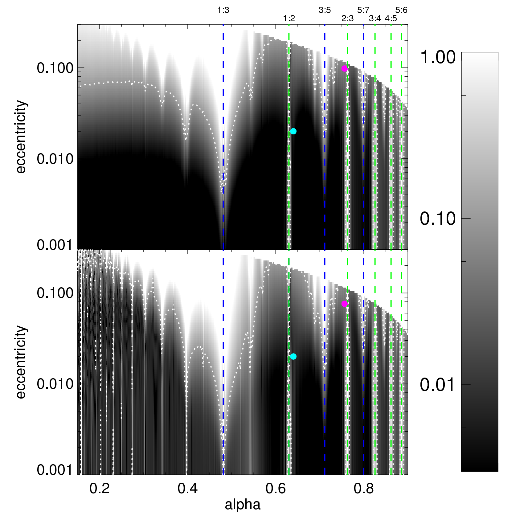
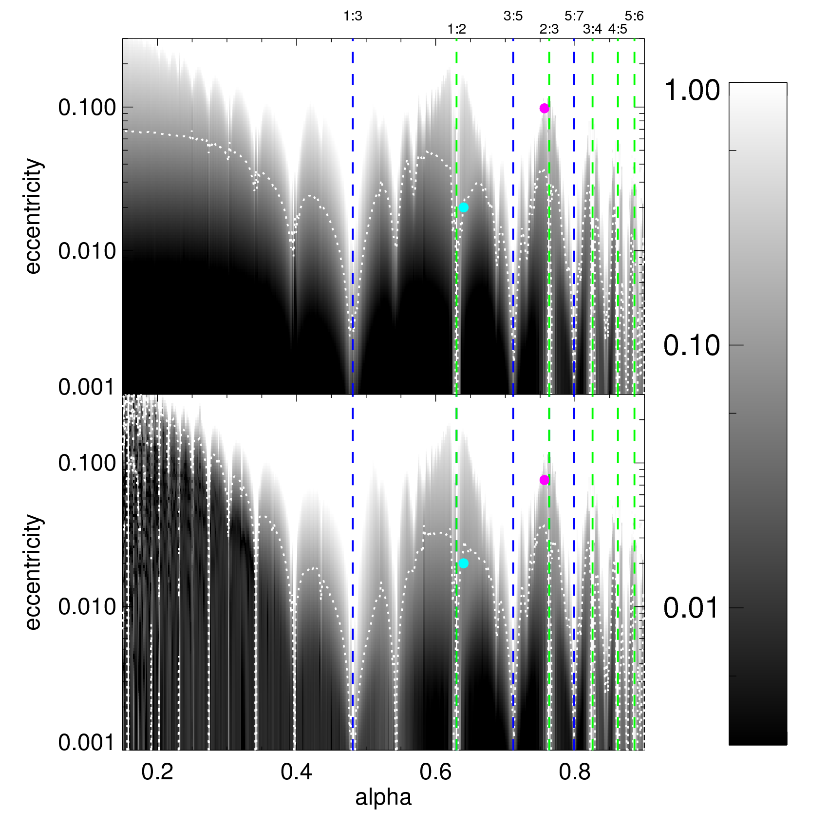
Figure 4.— Fractional precision of the analytic formula compared with TTVFast. Left: Aligned longitudes of periastron ($\varpi_{1}=\varpi_{2}$); Right: Anti-aligned longitudes of periastron ($\varpi_{1}=\varpi_{2}+\pi$). The dotted lines indicate the 10% precision level. Cyan dots show the approximate position of Kepler-18b/c at the 85.15% posterior eccentricity value, while magenta is used for Kepler-28. The region in the upper right is Hill unstable; these models were not computed, and default to 100% uncertainty in this plot. The green dashed lines show the locations of $j$:$j+1$ resonances, while the blue dashed lines show $j$:$j+2$.

3.2.2 Mass dependence

We have carried out simulations for a range of masses, keeping $m_{1}=m_{2}(\mu_{1}=\mu_{2})$. We find that the fractional error of the analytic formula grows near resonances and near $\alpha=1$ as the mass increases with weaker dependence upon eccentricity. For small $\alpha$, the formula works well up to $m_{1}=m_{2}=10^{-3}m_{\star}$, while near $1$:$2$ period ratio, for example, the error broadens around the resonance.

Figure 5 shows the fractional error in the formula (computed as in the eccentricity dependent case) for $e_{1}=e_{2}=0.001$ (the mass dependence of the precision is nearly independent of eccentricity) with $\varpi_{1}=\varpi_{2}+\pi$ (the results look very similar for $\varpi_{1}=\varpi_{2}$). The formula is accurate for a broad range of masses, but for some systems, such as Planet Hunters 3c/d, indicated in Cyan in Fig. 5, the discrepancy becomes large, $\approx 10$% (the masses and eccentricity vectors for this plot differ from PH3c/d, but a plot made for the parameters of that pair of planets looks very similar).

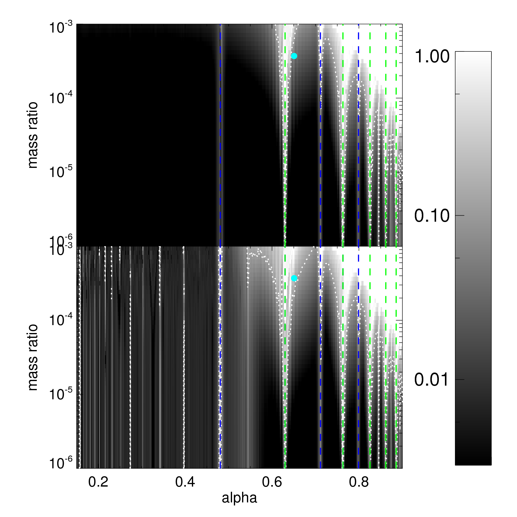
Figure 5.— Fractional precision of the analytic formula compared with TTVFast versus $\alpha$ and mass ratio of the planets to the star ($m_{1}=m_{2}$). Top: inner planet; bottom: outer planet. The dotted line indicates the 10% precision level. Cyan dots show the approximate position of PH3 (although note that PH3 does not have equal masses; however, the plot is similar for parameters appropriate for PH3). The region in the upper right is Hill unstable; these models were not computed, and default to 100% uncertainty in this plot. The green dashed lines show the locations of $j$:$j+1$ resonances, while the blue dashed lines show $j$:$j+2$.

3.3. Comparison with two-planet systems

We have carried out fits to systems with two interacting planets described in LXW12, and we have re-fit Planet Hunters (PH3) c/d. We have carried out N-body dynamical analyses using TTVFast in addition to fits with the analytic first-order formula in order to assess its utility in analyzing multi-planet systems.

Our first case is Kepler-18c/d, which was published by Cochran et al. (2011) and also analyzed by LXW12. We used the same transit times and uncertainties from the Cochran et al. (2011) paper to allow for direct comparison to their results; these transit times were also used in LXW12. We carried out a markov chain monte carlo (MCMC) analysis using an affine-invariant population approach (Goodman & Weare, 2010). We allow a multiplicative factor for the timing uncertainties on each planet and we place a uniform prior on the eccentricity of each planet (Ford, 2006). Figure 6 shows a comparison of the results of the MCMC analyses with N-body integration versus the analytic formulae with $j_{max}=5$. For this system the mass ratios are $\approx 5\times 10^{-5}$ and the eccentricities are of order $0-0.02$ (1-$\sigma$), while $\alpha\approx 0.64$, which is a regime in which the first-order formula is accurate to $<$9% compared with N-body integration (see Figure 4; the cyan dot indicates the approximate location of the upper end of the eccentricities of Kepler-18c/d). For conversion of the mass ratios to planet masses, we assume that $m_{\star}=0.972M_{\odot}$ (we ignore the uncertainty on this stellar mass). The masses of the planets derived from N-body are $m_{1}(nbody)=14.7_{-6.7}^{+5.4}M_{\oplus}$ and $m_{2}(nbody)=14.3_{-4.1}^{+2.3}M_{\oplus}$, while from the analytic formula are $m_{1}(analytic)=13.2_{-7.0}^{+5.4}M_{\oplus}$ and $m_{2}(analytic)=13.6_{-4.9}^{+2.4}M_{\oplus}$. These are well within $1-\sigma$ of one another, the markov chain posteriors show very similar distributions (Fig. 6). We note that these results differ from those reported by Cochran et al. (2011) who used N-body to estimate the transit times, found the best fit using Levenberg-Marquardt optimization, and estimated the uncertainties from the Hessian matrix at the best fit parameters rather than a full posterior analysis. Our results also differ from the estimates in LXW12, which only solve for a ‘nominal’ mass assuming zero eccentricity using the approximate near-resonant formula. We feel that our results should be superior to these prior results, and warrant a more extensive analysis with the full Kepler dataset as well as radial velocity measurements.

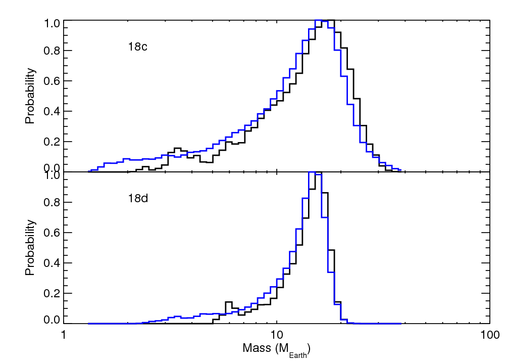
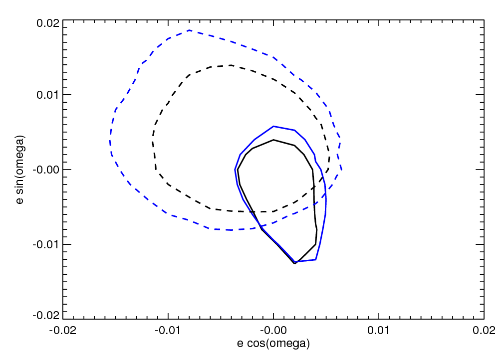
Figure 6.— Comparison of numerical and analytic analysis of the transit times of Kepler-18. Left: histogram of the masses of each planet. Right: comparison of the 68% confidence distribution of the eccentricity vectors of the two planets (18c solid; 18d dashed). In each case black indicates the results from the N-body analysis, while blue indicates the results of the analytic formula.

We next compared analyses of the Kepler-28 system, which was originally studied by Steffen et al. (2012), and included in the analysis of LXW12. We used the transit times published by Steffen et al. (2012), and followed the same procedure as Kepler-18. Figure 7 shows a comparison of the masses and eccentricity vectors for this system, which has a mean period ratio of $\langle P_{2}/P_{1}\rangle=1.52$, just wide of 2:3 period ratio, corresponding to $\alpha=0.7563$. The masses are poorly constrained due to the degeneracy with eccentricity, which allows the eccentricity to wander to larger values. For conversion of the mass ratios to planet masses, we assume that $m_{\star}=0.89M_{\odot}$ (we ignore the uncertainty on this stellar mass). A comparison between the mass constraints from N-body and the analytic formula gives: $m_{1}(nbody)=3.8_{-2.3}^{+4.6}M_{\oplus}$ versus $m_{1}(analytic)=3.1_{-1.7}^{+3.4}M_{\oplus}$, and $m_{2}(nbody)=5.1_{-3.0}^{+5.9}M_{\oplus}$ versus $m_{2}(analytic)=4.1_{-2.3}^{+4.6}M_{\oplus}$. The 85% confidence value of $e_{1}$ is 0.098, while for $e_{2}$ is 0.076, while the longitudes of periastron within the posterior distribution are primarily anti-aligned; the location of these points is indicated with a magenta datapoint in Figure 4. Note that in the anti-aligned $\varpi$ case the analytic formula is valid to larger eccentricities, and thus is adequate to describe this system.

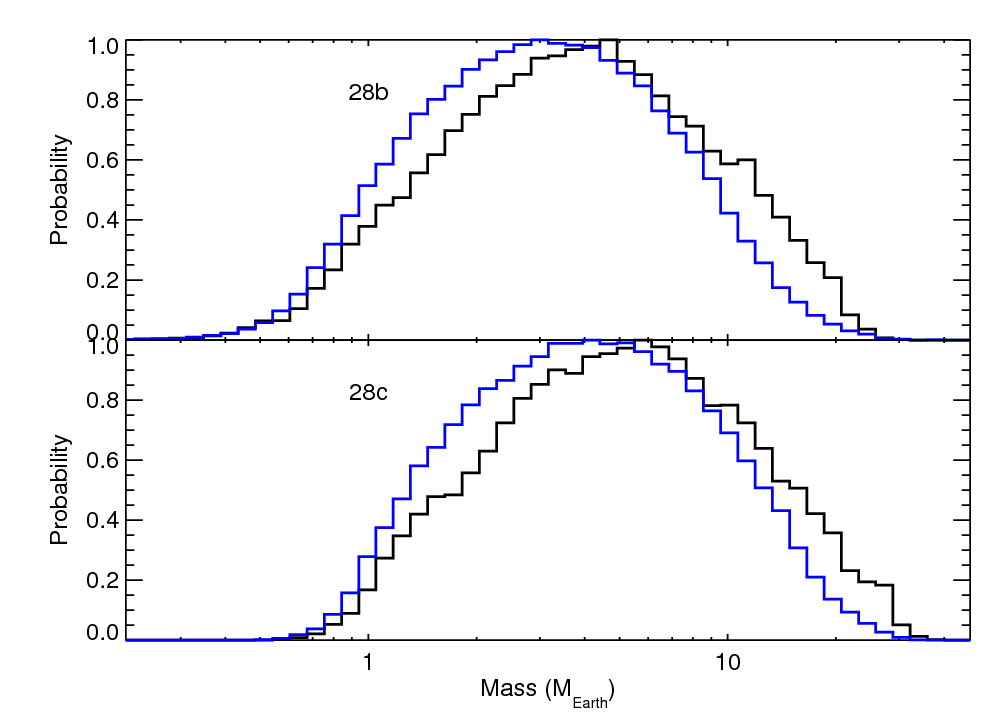
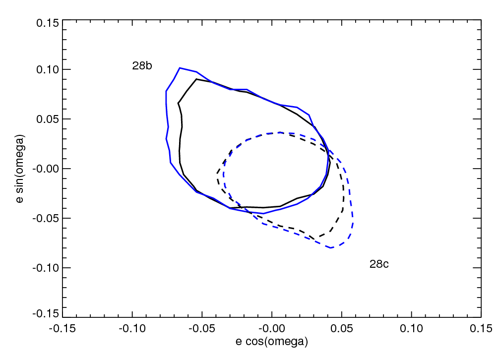
Figure 7.— Comparison of numerical and analytic analysis of the transit times of Kepler-28. Left: histogram of the masses of each planet. Right: comparison of the 68% confidence distribution of the eccentricity vectors of the two planets (28b solid; 28c dashed). In each case black indicates the results from the N-body analysis, while blue indicates the results of the analytic formula.

As Figure 5 indicates, the Planet Hunters 3 (PH3) system, the outer two planets (c/d) analyzed in Deck & Agol (2015), has a large discrepancy due to the large mass of the outer planet. The excellent agreement with the chopping formula given in Deck & Agol (2015) is still imperfect; the figure in that paper was mistakenly produced with larger timing error bars than used in Schmitt et al. (2014) which caused the agreement to appear slightly better than the first-order formula indicates. Figure 8 shows the results of a comparison of N-body and analytic fits to the PH3 transit times given in Schmitt et al. (2014); the planet masses assume $m_{\star}=1M_{\odot}$. The analytic formula gives a significant discrepancy due to the large mass of the outer planet and due to the proximity to the 1:2 period ratio.

To confirm that the large mass of PH3d led to this discrepancy, we took the best-fit parameters resulting from our N-body analysis of the real PH3 data, and reduced the masses of the outer two planets by a factor of 10. Using the outer two planets alone, we simulated transit times and added Gaussian noise at a level of $1/10$ that of the noise of the real data to maintain the same signal-to-noise ratio as the actual data. We then modeled this simulated data using TTVFast and the analytic formulae. We found that the agreement between the N-body and analytic analyses becomes excellent (Fig. 8).

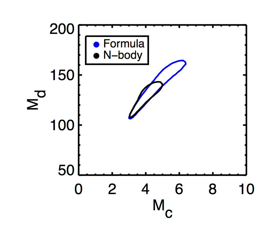
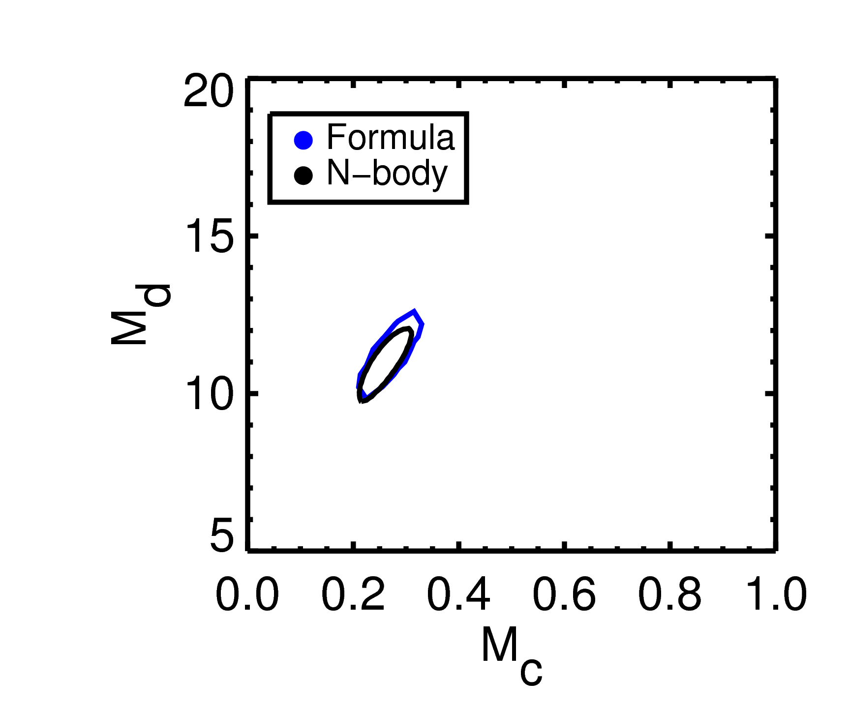
Figure 8.— Comparison of numerical and analytic analysis of the transit times of Planet Hunters 3c/d. Left: 68% confidence contour of the masses of both planets. Right: comparison of the 68% confidence limits with the mass of the both planets reduced by a factor of 10.

3.4. Comparison with multi-planet systems

The two-body solution can be used for more than two bodies by addition of two-body TTV solutions for each pair of two planets (Lissauer et al., 2011):

$$\delta t_{i_{1}}=\sum_{i_{2}\neq i_{1}}\delta t_{i_{1},i_{2}},$$ (21)

where $\delta t_{i_{1},i_{2}}$ are the solutions from equation (12) for the $i_{1}$th planet due to the $i_{2}$th planet. The sum over $j$ for each pair of planets can be carried up to $j_{max}$ to give sufficient precision for that pair of planets that is smaller than the measured timing precision.

Our first system of study is Kepler-51 (Masuda, 2014), consisting of planets with period ratios close to 1:2:3. We used the transit times reported in Masuda (2014) to carry out dynamical models with N-body/TTVFast and with an analytic TTV signal given as the sum of the TTVs of the three adjacent pairs of planets. We included up to $j=6$ in the TTV signals. The results show excellent agreement; Figure 9 shows the measured transit-timing variations, as well as the best-fit N-body and analytic TTVs. The results of the MCMC analyses are compared in Figure 10 which shows the posterior distribution of masses and eccentricities measured with both analyses, assuming $m_{\star}=1M_{\odot}$. For two of the planets the eccentricities are consistent with zero; in these cases the tail of the eccentricity histogram is heavier for the N-body than the for the analytic formula. The masses of the inner two planets from our N-body and analytic MCMC analyses agree well with the masses from the analysis in Masuda (2014), while the mass of the outer planet is small by $\approx 1-\sigma$.

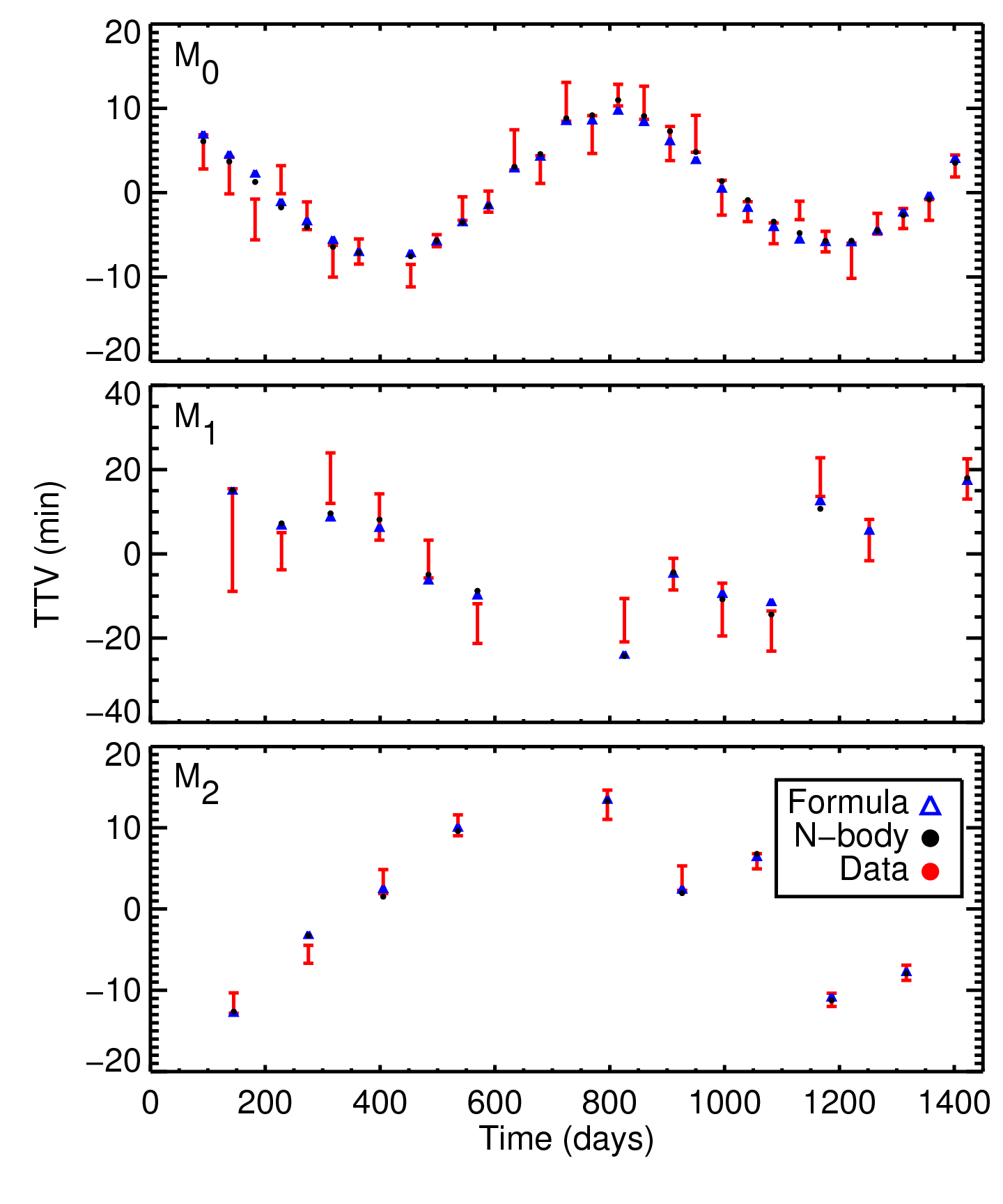
Figure 9.— Transit timing variations from Masuda (2014) for Kepler-51 (red; 0, 1, 2 stand for 51b,c, 620.02), compared with the best-fit N-body model computed with TTVFast (black), and the best-fit two-planet, first-order eccentricity formula summed over pairs of planets (blue).

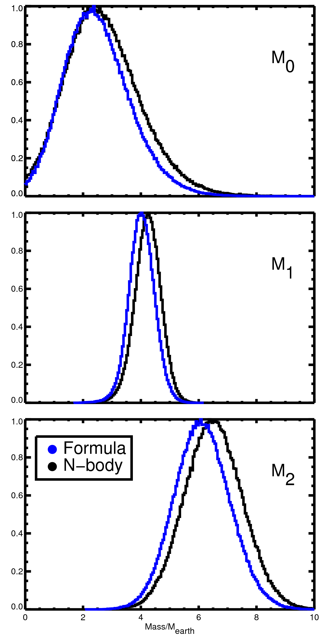
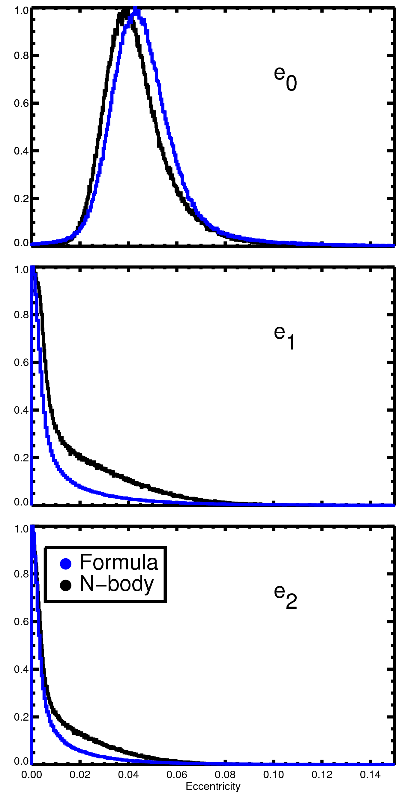
Figure 10.— Comparison of numerical and analytic analyses of the transit times of Kepler-51 (0, 1, 2 stand for 51b,c, 620.02). Left: histograms of the masses of each planet. Right: histograms of the eccentricities of the planets.

4. Numerical implementation and speed

The primary computational burden of equation (12) lies in computing the Laplace coefficients. We use a series solution for these coefficients, which gives both speed and accuracy, using code shared by Jack Wisdom. The secondary computational burden is in computing the sine and cosine terms, which involves four angles, and thus requires eight evaluations. We carry out the computation of higher $j$ sines and cosines using trigonometric addition formulae, which means we only need to compute eight trigonometric functions at each transit time once; the rest are gotten from addition and multiplication of these.

In the cases that we run a Markov chain for a set of planets, the initial value of $\alpha$ is known fairly well from the period ratio of the planets. In this case the Laplace coefficients and their derivatives needed for the solution can be Taylor expanded at the $\alpha$ given by an initial fit to the transit times, and these coefficients can be stored for evaluation of the coefficients at slightly different values of $\alpha$ encountered during the MCMC simulation. This approach would not work if $\alpha$ is being varied over a grid (for example, in the case of searching for a perturbing planet with unknown period); however, computational efficiency can still be achieved by reusing the Laplace coefficients at different eccentricities (Nesvorný & Morbidelli, 2008).

We have coded the first-order formula, equation (12), in C, IDL, Python, and Julia (Bezanzon et al., 2012). We carried out a benchmark comparison of the Julia implementation of the formula with the C implementation of TTVFast, and we find that it is $400\times$ faster when the Laplace coefficients are approximated from a Taylor expansion. As TTVFast is about 20 times faster than TTVs computed with standard N-body integrators, this represents nearly four orders of magnitude in speed up, similar to that found by Nesvorný & Morbidelli (2008). Note that if integer period ratios are chosen, sometimes the denominators of $u$ and $v_{\pm}$ can become infinite, causing divergence; we expect that this will not be encountered in practice as the formulae only apply to non-resonant planets.

The code implementing these equations may be accessed at https://github.com/ericagol/TTVFaster.

5. Discussion and conclusions

In modeling transit timing variations, degeneracies and computational speed can each prohibit the accurate measurement of transiting planet masses and orbital properties, with their attendant uncertainties. The degeneracy due to aliasing near first order resonances (LXW12) can be broken with very high signal-to-noise due to the slight difference in the eccentricity dependence as a function of period ratio, as well the presence of perturbations at other frequencies (Deck & Agol, 2015). Here we have tried to improve the modeling of the terms which are linearly dependent upon eccentricity to provide a higher-fidelity analytic model to address both the degeneracy and the computation barriers.

To this end, we have presented a first-order solution in eccentricity and mass ratio to the plane-parallel, near-circular 3-body problem on timescales shorter than the secular timescale. This improves to first order in eccentricity the original solution given in Agol et al. (2005) which was derived to zeroth order in eccentricity and first order in mass ratio (this solution has also been given in different forms in Nesvorný & Vokrouhlický 2014 and Deck & Agol 2015). The expressions are accurate compared with numerical integration over a wide range of parameter space relevant to the hundreds of multi-transiting planetary systems being found at short orbital periods with Kepler (Rowe et al., 2014; Lissauer et al., 2014). We find that this expression is more accurate than the stripped-down near-resonant formula given in LXW12, although their formula has a simpler form which clearly highlights the mass-eccentricity degeneracy. The first-order eccentricity formulae also can be used to model more than two planets with linear combinations of 2-planet formulae, and works well for the system we tested here, Kepler-51.

We used an approach starting with the Newtonian equations of motion rather than the Hamiltonian, and compute the perturbed polar coordinates of the planets’ orbits; this approach is akin to solving dispersion relations of differential equations for mode and stability analysis (for example, the magneto-rotational instability is derived with this approach, Chandrasekhar 1961; Balbus & Hawley 1998). The unperturbed solution to these differential equations represents Keplerian motion expanded in eccentricity. The terms with various frequencies in the disturbing function give an inhomogeneous component to the solution, which cause TTVs to vary at frequencies which depend upon integer combinations of the orbital frequencies of the two planets. Since the answer obtained in the end is the same as in the Hamiltonian (for ${\cal O}(e^{0})$) and canonical transformation approaches, this approach might be useful pedagogically for those more familiar with stability analyses. In addition, this approach might be useful for other problems, such as a stability analysis of a two-planet system or for carrying out the TTV computation to second-order in mass ratios $\mu_{i}=m_{i}/m_{\star}$. The latter is interesting as it would reveal how TTVs of a transiting planet may be used to measure the mass of that planet (and not just the mass of the perturbing planet).

We expect that these formulae will be used in carrying out initial fits to multi-transiting planets which show TTVs (Mazeh et al., 2013), in searching for companion perturbing planets to isolated planets showing TTVs, in characterizing multi-planet systems with TTVs to confirm and check for convergence of N-body MCMC analyses, in forecasting TTV amplitude for follow-up measurement, in estimating the optimum times for transit observation, and in making predictions for transit times to plan observations. It should be useful for estimating the densities, masses, and radii of the host stars and their exoplanets (Agol et al., 2005; Montet & Johnson, 2012; Hadden & Lithwick, 2014; Kipping et al., 2014; Jontof-Hutter et al., 2015), and in comparing the TTV solutions to radial velocity solutions for the masses and orbits of exoplanets. The analytic nature of our solution should be amenable to automatic differentiation (Fournier et al., 2012), which could speed up optimization based on gradient computation, and could also enable Hamiltonian/Hybrid Markov Chain Monte Carlo (Neal, 2011). When a large number of planets transit a star and each show evidence for dynamical interactions, the number of free parameters describing the system becomes large, and thus MCMC becomes prohibitively computationally expensive. The first-order analytic formula developed here can be used for modeling these systems if their masses and eccentricities are in the allowable range. As the formula is about 400 times faster than TTVFast, which is already about 20 times faster than Bulirsch-Stoer based integrators, the total speedup of about 8000 should make running chains long enough to converge more feasible, especially in tandem with parallel computation which can be easily adapted for population MCMC (Foreman-Mackey et al., 2013). The analytic formula also has the advantage of being able to pinpoint which features in the TTVs constrain the parameters of the system (LWX12). Since the TTVs of a planet display harmonics of the perturbing planet (Deck & Agol, 2015), the amplitudes and phases of each of these harmonics can be measured directly from the TTVs, and then these can be used to place individual constraints upon the masses and eccentricity vectors of the planets. The regions where the constraints overlap may reveal the consistency and uniqueness of the solution for the system parameters in some cases (Deck & Agol, 2015).

Although in principle TTVs allow for unique measurements of planet mass and eccentricities, degeneracies between these parameters are often found for systems with low signal to noise. In these cases, the eccentricities can become extremely large, indicating unstable orbits, as long as the masses are adjusted in a corresponding manner. We applied Hill stability to avoid this problem when using the analytic formulae; the full N-body computation avoids this issue naturally since large eccentricities introduce second-order (and higher) variations (that our calculation ignores) which prevent the high-eccentricity cases from fitting the data well. It may be possible to break some degeneracies with transit duration variations (Pál & Kocsis, 2008; Nesvorný et al., 2013), which can be computed with the same formalism we have described here, albeit in the plane-parallel limit.

The first-order formulae described here could be extended to higher order in eccentricity and/or mass ratio, albeit with much more computational effort. A slightly more accurate formula might be obtained by computing the longitudes from Kepler’s equation at the times of transit of each planet rather than using the first-order eccentricity formula (11), as well as using the exact formula for $\dot{\theta}_{i}$ at the transit times in equation (1); this requires very little additional computational effort, but $\delta\theta_{i}$ will still be only accurate to first order in eccentricity. The solutions for the perturbed polar coordinates, $(\delta r_{i},\delta\theta_{i})$, can be derived in the same manner that we have derived the transit timing variations. These are needed for carrying out the higher-order perturbation solutions, and in turn could be used for modeling astrometric variations, radial velocity varations, and pulsar timing variations of host stars to account for the interactions of planets to first order in eccentricity.

APPENDIX A

A new approach to TTVs

Here we give the detailed derivation of the first-order solution presented in Section 2.

5.1. TTVs from angular and radial variations

We start with the equations of motion in Murray & Dermott (MD), 6.10-6.11, which are in heliocentric coordinates. We use the index $i$ to label the planets, and denote the inner planet with $i=1$ and outer with $i=2$. TTVs can be computed from the true longitudes, $\theta_{1}$ and $\theta_{2}$, with respect to the star; hence heliocentric coordinates are ideal for transit timing computation. We convert the equations of motion to polar coordinates, and isolate the radial and longitudinal equations:

$$r_{i}^{2}\ddot{\theta}_{i}+2r_{i}\dot{r}_{i}\dot{\theta}_{i} = \frac{\partial}{\partial\theta_{i}}(U_{i}+{\cal R}_{i})=\frac{\partial{\cal R}_{i}}{\partial\theta_{i}}=\dot{l}_{i},$$ (22)

$$\ddot{r_{i}}-r_{i}\dot{\theta}_{i}^{2} = \frac{\partial}{\partial r_{i}}\left(U_{i}+{\cal R}_{i}\right).$$ (23)

The first equation can be rewritten as the time derivative of specific angular momentum, $l_{i}$, and without the disturbing force it expresses conservation of angular momentum, while the second equation includes centripetal acceleration in the radial direction as the second term on the left hand side. The term $U_{i}=G(m_{\star}+m_{i})/r_{i}$ is the standard Keplerian potential, while ${\cal R}_{i}$ is the disturbing function which reflects the gravitational potential energy of planet-planet interactions. Because the planet-planet interactions lead to only small perturbations of the base Keplerian orbits, we seek a solution to equations (22) of the form: $r_{i}=r_{i,K}+\delta r_{i}$ and $\theta_{i}=\theta_{i,K}+\delta\theta_{i}$, where $(r_{i,K},\theta_{i,K})$ is the unperturbed Keplerian polar coordinates of the orbits, and $(\delta r_{i},\delta\theta_{i})$ are the small perturbations. We can then plug these solutions into the equations of motion (22) and expand in powers of $\delta r_{i},\delta\theta_{i}$, mass ratio, and eccentricity.

We normalize $r_{i}$ by $a_{i}$, which is the semi-major axis of the unperturbed Keplerian orbit (we do not perturb $a_{i}$, $\varpi_{i}$, or $e_{i}$, so they are fixed at the mean, unperturbed values). Then $r_{i}/a_{i}=1+\epsilon_{i}$, where $\epsilon_{i}$ is a dimensionless radial coordinate, so that $\dot{r}_{i}/a_{i}=\dot{\epsilon}_{i}$ and $\delta r_{i}/a_{i}=\delta\epsilon_{i}$. The solution to the unperturbed orbits to first order in eccentricity is $\theta_{i,K}=\lambda_{i}-Re\left[2\mathbbm{i}z_{i}^{*}e^{\mathbbm{i}\lambda_{i}}\right]=\lambda_{i}+2e_{i}\sin{(\lambda_{i}-\varpi_{i})}$ and $\epsilon_{i,K}=-Re\left[z_{i}^{*}e^{\mathbbm{i}\lambda_{i}}\right]$ where $\mathbbm{i}=\sqrt{-1}$, $z_{i}=e_{i}e^{\mathbbm{i}\varpi_{i}}=e_{i}(\cos{\varpi_{i}}+\mathbbm{i}\sin{\varpi_{i}})$ is the complex eccentricity vector (LXW12), $z^{*}$ is the complex conjugate of $z$, and $Re[.]$ is the real part.

5.2. Perturbed equations of motion

The perturbed equations become:

$$r_{i,K}^{2}\delta\ddot{\theta}_{i} = -2r_{i,K}\ddot{\theta}_{i,K}\delta r_{i}-2\dot{r}_{i,K}\dot{\theta}_{i,K}\delta r_{i}-2r_{i,K}\dot{\theta}_{i,K}\delta\dot{r}_{i}-2r_{i,K}\dot{r}_{i,K}\delta\dot{\theta}_{i}+\frac{\partial{\cal R}_{i}}{\partial\theta_{i}},$$ (24)

$$\delta\ddot{r_{i}} = 2r_{i,K}\dot{\theta}_{i,K}\delta\dot{\theta}_{i}+\dot{\theta}_{i,K}^{2}\delta r_{i}+\frac{2G(m_{\star}+m_{i})}{r_{i,K}^{3}}\delta r_{i}+\frac{\partial{\cal R}_{i}}{\partial r_{i}}.$$ (25)

In these equations, we have cancelled the terms for the unperturbed Keplerian on both sides of the equation. From hereon we will drop the ‘$K$’ subscript from the unperturbed Keplerian orbital elements. To first order in eccentricity, the TTVs of the $i$th planet are:

$$\delta t_{i}=-n_{i}^{-1}(\delta\theta_{i}+2\epsilon_{i}\delta\theta_{i}^{(0)}),$$ (26)

where $\delta\theta_{i}^{(0)}$ is the perturbed solution to zeroth order in eccentricity. To lowest order in eccentricity, $\epsilon_{i}=-e_{i}\cos{(\lambda_{i}-\varpi_{i})}$, so:

$$\epsilon_{i} = -\tfrac{1}{2}\left(e_{i}e^{\mathbbm{i}(\lambda_{i}-\varpi_{i})}+e_{i}e^{-\mathbbm{i}(\lambda_{i}-\varpi_{i})}\right)$$ (27)

$$\dot{\epsilon}_{i} = -\tfrac{\mathbbm{i}n_{i}}{2}\left(e_{i}e^{\mathbbm{i}(\lambda_{i}-\varpi_{i})}-e_{i}e^{-\mathbbm{i}(\lambda_{i}-\varpi_{i})}\right).$$ (28)

5.3. First order in eccentricity equations

Let the specific angular momentum equal $l_{i}=r_{i}^{2}\dot{\theta}_{i}$. Since $l_{i}$ is a constant, $\ddot{\theta}_{i}=-2l_{i}\dot{r}_{i}/r_{i}^{3}$. To first order in eccentricity, $l_{i}=n_{i}a_{i}^{2}$, where $n_{i}=2\pi/P_{i}$. Substituting these into the above equations, and expanding to first order in eccentricity, we find

$$\delta\ddot{\epsilon}_{i}-2n_{i}(1-\epsilon_{i})\delta\dot{\theta}_{i}-n_{i}^{2}(3-10\epsilon_{i})\delta\epsilon_{i} = \frac{1}{a_{i}^{2}}\frac{\partial{\cal R}_{i}}{\partial\epsilon_{i}}$$ (29)

$$(1+2\epsilon_{i})\delta\ddot{\theta}_{i}-2n_{i}\dot{\epsilon}_{i}\delta\epsilon_{i}+2n_{i}(1-\epsilon_{i})\delta\dot{\epsilon}_{i}+2\dot{\epsilon}_{i}\delta\dot{\theta}_{i} = \frac{1}{a_{i}^{2}}\frac{\partial{\cal R}_{i}}{\partial\theta_{i}}.$$ (30)

Note that the terms with $\epsilon_{i}$ or $\dot{\epsilon}_{i}$ are first order in eccentricity; hence, the other quantities in these terms need to only be expanded to zeroth order in eccentricity. Denoting the zeroth-order solutions as $\delta\epsilon_{i}^{(0)}$ and $\delta\theta_{i}^{(0)}$, we find the differential equations governing the transit timing solution:

$$\delta\ddot{\theta}_{i}+2n_{i}\delta\dot{\epsilon}_{i} = -2\left(\epsilon_{i}\delta\ddot{\theta}_{i}^{(0)}+\dot{\epsilon}_{i}\delta\dot{\theta}_{i}^{(0)}\right)+2n_{i}\left(\dot{\epsilon}_{i}\delta\epsilon_{i}^{(0)}+\epsilon_{i}\delta\dot{\epsilon}_{i}^{(0)}\right)+\frac{1}{a_{i}^{2}}\frac{\partial{\cal R}_{i}}{\partial\theta_{i}},$$ (31)

$$\delta\ddot{\epsilon}_{i}-3n_{i}^{2}\delta\epsilon_{i}-2n_{i}\delta\dot{\theta}_{i} = -2n_{i}\epsilon_{i}\left(\delta\dot{\theta}_{i}^{(0)}+5n_{i}\delta\epsilon_{i}^{(0)}\right)+\frac{1}{a_{i}^{2}}\frac{\partial{\cal R}_{i}}{\partial\epsilon_{i}}.$$ (32)

We assume that both sides of these equations are complex, and the final solution is found from taking their real parts.

The quantity ${\cal R}_{i}$ is the disturbing function, which for the inner planet can be broken into two pieces: ${\cal R}_{1}=\frac{Gm_{2}}{a_{2}}({\cal R}_{D}+\alpha{\cal R}_{E})$ (MD 6.44), where ${\cal R_{D}}=a_{2}/|{\bf r}_{2}-{\bf r}_{1}|$ and ${\cal R}_{E}=-(r_{1}/a_{1})(a_{2}/r_{2})^{2}\cos{(\theta_{1}-\theta_{2})}$. For the outer planet, there are also two pieces, ${\cal R}_{2}=\frac{Gm_{1}}{a_{2}}({\cal R}_{D}+\alpha^{-2}{\cal R}_{I})$, where ${\cal R}_{I}=-(1+\epsilon_{2})(1+\epsilon_{1})^{-2}\cos{(\theta_{1}-\theta_{2})}$ (MD 6.45). As usual, $\alpha=a_{1}/a_{2}\approx(P_{1}/P_{2})^{2/3}$.

5.4. Expansion of the disturbing functions

The expansion for ${\cal R}_{D}$ is given in MD 6.66. We are considering the plane-parallel case, so $\Psi=\cos{\psi}-\cos{(\theta_{1}-\theta_{2})}=0$, in which case we only need to include the $\propto\Psi^{0}$ term. Also, we would like a solution that is first order in eccentricity (of the unperturbed Keplerian orbit), so the term in brackets in MD 6.66 needs to be expanded to second order in $\epsilon_{i}=\frac{r_{i}}{a_{i}}-1$ (noting again that $\epsilon_{i}$ is first order in eccentricity):

$$\sum_{l=0}^{2}\frac{1}{l!}\sum_{k=0}^{l}{l\choose k}\epsilon_{1}^{k}\epsilon_{2}^{l-k}A_{0,j,k,l-k}=A_{0,j,0,0}+A_{0,j,1,0}\epsilon_{1}+A_{0,j,0,1}\epsilon_{2}+\frac{1}{2}A_{0,j,0,2}\epsilon_{2}^{2}+A_{0,j,1,1}\epsilon_{1}\epsilon_{2}+\frac{1}{2}A_{0,j,2,0}\epsilon_{1}^{2},$$ (33)

where $A_{0,j,m,n}=a_{1}^{m}a_{2}^{n}\frac{\partial^{m+n}}{\partial a_{1}^{m}\partial a_{2}^{n}}\left(a_{2}^{-1}b_{1/2}^{(j)}(\alpha)\right)$ (MD 6.63) and $b_{s}^{(j)}$ is a Laplace coefficient (MD 6.67). We define $\tilde{A}_{jmn}=a_{2}A_{0,j,m,n}$ to simplify the expressions below.

We rewrite ${\cal R}_{D}$ in complex notation (in the plane-parallel limit, expanded to second order in $\epsilon_{i}$), giving:

$${\cal R}_{D} = {\cal R}_{D,0}+Re\Bigg{[}\sum_{j\geq 1}\left(\tilde{A}_{j00}+\tilde{A}_{j10}\epsilon_{1}+\tilde{A}_{j01}\epsilon_{2}+\frac{1}{2}\tilde{A}_{j02}\epsilon_{2}^{2}+\tilde{A}_{j11}\epsilon_{1}\epsilon_{2}+\frac{1}{2}\tilde{A}_{j20}\epsilon_{1}^{2}\right)e^{\mathbbm{i}j(\theta_{1}-\theta_{2})}\Bigg{]},$$ (34)

$${\cal R}_{D,0} = \frac{1}{2}\left(\tilde{A}_{000}+\tilde{A}_{010}\epsilon_{1}+\tilde{A}_{001}\epsilon_{2}+\frac{1}{2}\tilde{A}_{002}\epsilon_{2}^{2}+\tilde{A}_{011}\epsilon_{1}\epsilon_{2}+\frac{1}{2}\tilde{A}_{020}\epsilon_{1}^{2}\right).$$ (35)

where we have used the fact that $A_{0,j,k,l}=A_{0,-j,k,l}$ since $b_{s}^{(j)}=b_{s}^{(-j)}$. Likewise,

$${\cal R}_{E}=-Re\bigg{[}(1+\epsilon_{1})(1+\epsilon_{2})^{-2}e^{\mathbbm{i}(\theta_{1}-\theta_{2})}\bigg{]}.$$ (36)

Taking the derivative of ${\cal R}_{D}$ and ${\cal R}_{E}$ with respect to $\theta_{1}$ gives to first order in $\epsilon_{1}$:

$$\frac{1}{a_{1}^{2}}\frac{\partial{\cal R}_{1}}{\partial\theta_{1}}=\frac{1}{a_{1}^{2}}\delta\dot{l_{1}}=n_{1}^{2}\mu_{2}\alpha Re\left[\sum_{j\geq 1}\left(\tilde{A}_{j00}+\tilde{A}_{j10}\epsilon_{1}+\tilde{A}_{j01}\epsilon_{2}-\alpha(1+\epsilon_{1}-2\epsilon_{2})\delta_{j1}\right)\mathbbm{i}je^{\mathbbm{i}j(\theta_{1}-\theta_{2})}\right],$$ (37)

where we have used $n_{i}^{2}=Gm_{\star}/a_{i}^{3}=$ and $\mu_{i}=m_{i}/m_{\star}$. The derivative of ${\cal R}_{1}$ with respect to $\epsilon_{1}$ is:

$$\frac{1}{a_{1}^{2}}\frac{\partial{\cal R}_{1}}{\partial\epsilon_{1}} = n_{1}^{2}\mu_{2}\alpha Re\Bigg{[}\frac{1}{2}\left(\tilde{A}_{010}+\tilde{A}_{011}\epsilon_{2}+\tilde{A}_{020}\epsilon_{1}\right)$$ (38)

$$+ \sum_{j\geq 1}\left(\tilde{A}_{j10}+\tilde{A}_{j11}\epsilon_{2}+\tilde{A}_{j20}\epsilon_{1}-\alpha(1-2\epsilon_{2})\delta_{j1}\right)e^{\mathbbm{i}j(\theta_{1}-\theta_{2})}\Bigg{]}.$$ (39)

For the outer planet,

$$\frac{1}{a_{2}^{2}}\frac{\partial{\cal R}_{2}}{\partial\theta_{2}}=\frac{1}{a_{2}^{2}}\delta\dot{l_{2}}=-n_{2}^{2}\mu_{1}Re\left[\sum_{j\geq 1}\left(\tilde{A}_{j00}+\tilde{A}_{j10}\epsilon_{1}+\tilde{A}_{j01}\epsilon_{2}-\alpha^{-2}(1+\epsilon_{2}-2\epsilon_{1})\delta_{j1}\right)\mathbbm{i}je^{\mathbbm{i}j(\theta_{1}-\theta_{2})}\right].$$ (40)

The derivative of ${\cal R}_{2}$ with respect to $\epsilon_{2}$ is:

$$\frac{1}{a_{2}^{2}}\frac{\partial{\cal R}_{2}}{\partial\epsilon_{2}} = n_{2}^{2}\mu_{1}Re\Bigg{[}\frac{1}{2}\left(\tilde{A}_{001}+\tilde{A}_{011}\epsilon_{1}+\tilde{A}_{002}\epsilon_{2}\right)$$ (41)

$$+ \sum_{j\geq 1}\left(\tilde{A}_{j01}+\tilde{A}_{j11}\epsilon_{1}+\tilde{A}_{j02}\epsilon_{2}-\alpha^{-2}(1-2\epsilon_{1})\delta_{j1}\right)e^{\mathbbm{i}j(\theta_{1}-\theta_{2})}\Bigg{]}.$$ (42)

The angles and radii in the derivatives of the disturbing function can be expanded to first order in eccentricity, yielding:

$$\frac{1}{a_{1}^{2}}\frac{\partial{\cal R}_{1}}{\partial\theta_{1}} = n_{1}^{2}\mu_{2}\alpha Re\bigg{[}\sum_{j\geq 1}\mathbbm{i}je^{\mathbbm{i}j\psi}\Big{(}\big{(}\tilde{A}_{j00}-\alpha\delta_{j1}\big{)}$$ (43)

$$+ \big{(}j\tilde{A}_{j00}-\tfrac{1}{2}\tilde{A}_{j10}-\tfrac{1}{2}\alpha\delta_{j1}\big{)}z_{1}^{*}e^{\mathbbm{i}\lambda_{1}}+\big{(}-j\tilde{A}_{j00}-\tfrac{1}{2}\tilde{A}_{j10}+\tfrac{3}{2}\alpha\delta_{j1}\big{)}z_{1}e^{-\mathbbm{i}\lambda_{1}}$$ (44)

$$+ \big{(}-j\tilde{A}_{j00}-\tfrac{1}{2}\tilde{A}_{j01}\big{)}z_{2}^{*}e^{\mathbbm{i}\lambda_{2}}+\big{(}j\tilde{A}_{j00}-\tfrac{1}{2}\tilde{A}_{j01}-2\alpha\delta_{j1}\big{)}z_{2}e^{-\mathbbm{i}\lambda_{2}}\Big{)}\bigg{]}.$$ (45)

$$\frac{1}{a_{1}^{2}}\frac{\partial{\cal R}_{1}}{\partial\epsilon_{1}} = n_{1}^{2}\mu_{2}\alpha Re\Bigg{[}\tfrac{1}{2}\tilde{A}_{010}-\tfrac{1}{2}\tilde{A}_{020}z_{1}e^{-\mathbbm{i}\lambda_{1}}-\tfrac{1}{2}\tilde{A}_{011}z_{2}e^{-\mathbbm{i}\lambda_{2}}+\sum_{j\geq 1}e^{\mathbbm{i}j\psi}\Bigg{(}\big{(}\tilde{A}_{j10}-\alpha\delta_{j1}\big{)}$$ (46)

$$+ \left(j\tilde{A}_{j10}-\tfrac{1}{2}\tilde{A}_{j20}-\alpha\delta_{j1}\right)z_{1}^{*}e^{i\lambda_{1}}+\left(-j\tilde{A}_{j10}-\tfrac{1}{2}\tilde{A}_{j20}+\alpha\delta_{j1}\right)z_{1}e^{-\mathbbm{i}\lambda_{1}}$$ (47)

$$+ \left(-j\tilde{A}_{j10}-\tfrac{1}{2}\tilde{A}_{j11}\right)z_{2}^{*}e^{i\lambda_{2}}+\left(j\tilde{A}_{j10}-\tfrac{1}{2}\tilde{A}_{j11}-2\alpha\delta_{j1}\right)z_{2}e^{-\mathbbm{i}\lambda_{2}}\Bigg{)}\Bigg{]}.$$ (48)

where $\psi=\lambda_{1}-\lambda_{2}$. We have also combined the $j=0$ eccentricity terms since $Re(z_{i}^{*}e^{\mathbbm{i}\lambda_{i}})=Re(z_{i}e^{-\mathbbm{i}\lambda_{i}})=\tfrac{1}{2}(z_{i}^{*}e^{\mathbbm{i}\lambda_{i}}+z_{i}e^{-\mathbbm{i}\lambda_{i}})$.

For the outer planet,

$$\frac{1}{a_{2}^{2}}\frac{\partial{\cal R}_{2}}{\partial\theta_{2}} = -n_{2}^{2}\mu_{1}Re\bigg{[}\sum_{j\geq 1}\mathbbm{i}je^{\mathbbm{i}j\psi}\Big{(}\big{(}\tilde{A}_{j00}-\alpha^{-2}\delta_{j1}\big{)}$$ (49)

$$+ \big{(}j\tilde{A}_{j00}-\tfrac{1}{2}\tilde{A}_{j10}-2\alpha^{-2}\delta_{j1}\big{)}z_{1}^{*}e^{\mathbbm{i}\lambda_{1}}+\big{(}-j\tilde{A}_{j00}-\tfrac{1}{2}\tilde{A}_{j10}\big{)}z_{1}e^{-\mathbbm{i}\lambda_{1}}$$ (50)

$$+ \big{(}-j\tilde{A}_{j00}-\tfrac{1}{2}\tilde{A}_{j01}+\tfrac{3}{2}\alpha^{-2}\delta_{j1}\big{)}z_{2}^{*}e^{\mathbbm{i}\lambda_{2}}+\big{(}j\tilde{A}_{j00}-\tfrac{1}{2}\tilde{A}_{j01}-\tfrac{1}{2}\alpha^{-2}\delta_{j1}\big{)}z_{2}e^{-\mathbbm{i}\lambda_{2}}\Big{)}\bigg{]}.$$ (51)

$$\frac{1}{a_{2}^{2}}\frac{\partial{\cal R}_{2}}{\partial\epsilon_{2}} = n_{2}^{2}\mu_{1}Re\Bigg{[}\tfrac{1}{2}\tilde{A}_{001}-\tfrac{1}{2}\tilde{A}_{011}z_{1}^{*}e^{\mathbbm{i}\lambda_{1}}-\tfrac{1}{2}\tilde{A}_{002}z_{2}^{*}e^{\mathbbm{i}\lambda_{2}}+\sum_{j\geq 1}e^{\mathbbm{i}j\psi}\Bigg{(}\big{(}\tilde{A}_{j01}-\alpha^{-2}\delta_{j1}\big{)}$$ (52)

$$+ \left(j\tilde{A}_{j01}-\tfrac{1}{2}\tilde{A}_{j11}-2\alpha^{-2}\delta_{j1}\right)z_{1}^{*}e^{i\lambda_{1}}+\left(-j\tilde{A}_{j01}-\tfrac{1}{2}\tilde{A}_{j11}\right)z_{1}e^{-\mathbbm{i}\lambda_{1}}$$ (53)

$$+ \left(-j\tilde{A}_{j01}-\tfrac{1}{2}\tilde{A}_{j02}+\alpha^{-2}\delta_{j1}\right)z_{2}^{*}e^{i\lambda_{2}}+\left(j\tilde{A}_{j01}-\tfrac{1}{2}\tilde{A}_{j02}-\alpha^{-2}\delta_{j1}\right)z_{2}e^{-\mathbbm{i}\lambda_{2}}\Bigg{)}\Bigg{]}.$$ (54)

5.5. Trial solution

The derivatives of the complex disturbing function contain terms that are proportional to $e^{\mathbbm{i}j\psi}$, $e^{\mathbbm{i}j\psi}e_{i}e^{\pm\mathbbm{i}(\lambda_{i}-\varpi_{i})}$ for $j\geq 0$. We treat these terms as harmonic driving terms, and solve the inhomogeneous partial differential equations term by term. We expand the complex solutions for $\delta\theta_{1}$ and $\delta\epsilon_{1}$ as trial solutions:

$$\delta\epsilon_{1} = \delta\epsilon_{1,0}^{(+2)}e_{2}e^{\mathbbm{i}(\lambda_{2}-\varpi_{2})}+\sum_{j\geq 1}\delta\epsilon_{1,j}e^{\mathbbm{i}j\psi}$$ (55)

$$\delta\theta_{1} = \delta\theta_{1,0}^{(+2)}e_{2}e^{\mathbbm{i}(\lambda_{2}-\varpi_{2})}+\sum_{j\geq 1}\delta\theta_{1,j}e^{\mathbbm{i}j\psi}$$ (56)

$$\delta\epsilon_{1,j} = \delta\epsilon_{1,j}^{(0)}+\sum_{k=1,2}\left(\delta\epsilon_{1,j}^{(+k)}e_{k}e^{\mathbbm{i}(\lambda_{k}-\varpi_{k})}+\delta\epsilon_{1,j}^{(-k)}e_{k}e^{-\mathbbm{i}(\lambda_{k}-\varpi_{k})}\right),$$ (57)

$$\delta\theta_{1,j} = \delta\theta_{1,j}^{(0)}+\sum_{k=1,2}\left(\delta\theta_{1,j}^{(+k)}e_{k}e^{\mathbbm{i}(\lambda_{k}-\varpi_{k})}+\delta\theta_{1,j}^{(-k)}e_{k}e^{-\mathbbm{i}(\lambda_{k}-\varpi_{k})}\right),$$ (58)

and

$$\delta\epsilon_{2} = \delta\epsilon_{2,0}^{(+1)}e_{1}e^{\mathbbm{i}(\lambda_{1}-\varpi_{1})}+\sum_{j\geq 1}\delta\epsilon_{2,j}e^{\mathbbm{i}j\psi}$$ (59)

$$\delta\theta_{2} = \delta\theta_{1,0}^{(+1)}e_{1}e^{\mathbbm{i}(\lambda_{1}-\varpi_{1})}+\sum_{j\geq 1}\delta\theta_{2,j}e^{\mathbbm{i}j\psi}$$ (60)

$$\delta\epsilon_{2,j} = \delta\epsilon_{2,j}^{(0)}+\sum_{k=1,2}\left(\delta\epsilon_{2,j}^{(+k)}e_{k}e^{\mathbbm{i}(\lambda_{k}-\varpi_{k})}+\delta\epsilon_{2,j}^{(-k)}e_{k}e^{-\mathbbm{i}(\lambda_{k}-\varpi_{k})}\right),$$ (61)

$$\delta\theta_{2,j} = \delta\theta_{2,j}^{(0)}+\sum_{k=1,2}\left(\delta\theta_{2,j}^{(+k)}e_{k}e^{\mathbbm{i}(\lambda_{k}-\varpi_{k})}+\delta\theta_{2,j}^{(-k)}e_{k}e^{-\mathbbm{i}(\lambda_{k}-\varpi_{k})}\right).$$ (62)

We also define the solutions to zeroth order in eccentricity as:

$$\delta\epsilon_{i}^{(0)} = \sum_{j\geq 1}\epsilon_{i,j}^{(0)}e^{\mathbbm{i}j\psi}$$ (63)

$$\delta\theta_{i}^{(0)} = \sum_{j\geq 1}\theta_{i,j}^{(0)}e^{\mathbbm{i}j\psi}.$$ (64)

Then, the (real) transit timing variations are equal to

$$\delta t_{1} = -n_{1}^{-1}Re(\delta\theta_{1}+2\epsilon_{1}\delta\theta_{1}^{(0)})$$ (65)

$$= \delta t_{1,0}^{(-2)}+\sum_{j\geq 1}\left[\delta t_{1,j}^{(0)}+\sum_{k=1,2}\left(\delta t_{1,j}^{(+k)}+\delta t_{1,j}^{(-k)}\right)\right],$$ (66)

$$\delta t_{1,j}^{(0)} = -n_{1}^{-1}Re(\delta\theta_{1,j}^{(0)}e^{\mathbbm{i}j\psi})$$ (67)

$$\delta t_{1,j}^{(\pm k)} = -n_{1}^{-1}Re\left(\left(\delta\theta_{1,j}^{(\pm k)}-\delta\theta_{1,j}^{(0)}\delta_{k1}\right)e_{k}e^{\mathbbm{i}(j\psi\pm(\lambda_{k}-\varpi_{k}))}\right),$$ (68)

and

$$\delta t_{2} = -n_{2}^{-1}Re(\delta\theta_{2}+2\epsilon_{2}\delta\theta_{2}^{(0)})$$ (69)

$$= \delta t_{2,0}^{(+1)}+\sum_{j\geq 1}\left[\delta t_{2,j}^{(0)}+\sum_{k=1,2}\left(\delta t_{2,j}^{(+k)}+\delta t_{2,j}^{(-k)}\right)\right],$$ (70)

$$\delta t_{2,j}^{(0)} = -n_{2}^{-1}Re(\delta\theta_{2,j}^{(0)}e^{\mathbbm{i}j\psi})$$ (71)

$$\delta t_{2,j}^{(\pm k)} = -n_{2}^{-1}Re\left(\left(\delta\theta_{2,j}^{(\pm k)}-\delta\theta_{2,j}^{(0)}\delta_{k2}\right)e_{k}e^{\mathbbm{i}(j\psi\pm(\lambda_{k}-\varpi_{k}))}\right),$$ (72)

5.6. Inner planet coefficients

Substituting the $(j,{0,\pm k})$ trial solutions into the above differential equations, to zeroth order in eccentricity we find for the inner planet:

$$\begin{pmatrix}-\beta_{j}^{2}&2\mathbbm{i}\beta_{j}\\ -2\mathbbm{i}\beta_{j}&-(\beta_{j}^{2}+3)\end{pmatrix}\begin{pmatrix}\delta\theta_{1,j}^{(0)}\\ \delta\epsilon_{1,j}^{(0)}\end{pmatrix}=\mu_{2}\alpha\begin{pmatrix}\mathbbm{i}j(\tilde{A}_{j00}-\alpha\delta_{j1})\\ \tilde{A}_{j10}-\alpha\delta_{j1}\end{pmatrix}.$$ (73)

where $\beta_{j}=j(n_{1}-n_{2})/n_{1}=j(1-\alpha^{3/2})$ and we have divided the equations by $n_{1}^{2}$ to make dimensionless.

Similarly we can write down the equations for the coefficients to first order in $e_{1}$. Note that to solve for $\delta t_{1,j}^{(\pm 1)}$, we need to compute $\delta\theta_{1,j}^{(\pm 1)}-\delta\theta_{1,j}^{(0)}$. Hence we can subtract the matrix on the left times the vector $\left\{\delta\theta_{1,j}^{(0)},0\right\}$ from both sides of the equation. This may be rewritten in dimensionless form as:

$$\begin{pmatrix}-(\beta_{j}\pm 1)^{2}&2\mathbbm{i}(\beta_{j}\pm 1)\\ -2\mathbbm{i}(\beta_{j}\pm 1)&-((\beta_{j}\pm 1)^{2}+3)\end{pmatrix}\begin{pmatrix}\delta\theta_{1,j}^{(\pm 1)}-\delta\theta_{1,j}^{(0)}\\ \delta\epsilon_{1,j}^{(\pm 1)}\end{pmatrix}$$ (74)

$$= \begin{pmatrix}1\pm\beta_{j}&-\mathbbm{i}(\beta_{j}\pm 1)\\ \mathbbm{i}(3\beta_{j}\pm 2)&5\end{pmatrix}\begin{pmatrix}\delta\theta_{1,j}^{(0)}\\ \delta\epsilon_{1,j}^{(0)}\end{pmatrix}$$ (75)

$$+ \mu_{2}\alpha\begin{pmatrix}\mathbbm{i}j\left(\pm j\tilde{A}_{j00}-\tfrac{1}{2}\tilde{A}_{j10}+\tfrac{1}{2}\alpha\delta_{j1}(1\mp 2)\right)\\ \pm j\tilde{A}_{j10}-\tfrac{1}{2}\tilde{A}_{j20}\mp\alpha\delta_{j1}\end{pmatrix}.$$ (76)

The solutions of equation 73 for $(\delta\theta_{1,j}^{(0)},\delta\epsilon_{1,j}^{(0)})$ may be plugged into the first term on the right hand side of this equation to solve for the first order eccentricity terms.

To first order in $e_{2}$ in dimensionless form (for $j\geq 1$),

$$\begin{pmatrix}-\eta_{\pm}^{2}&2\mathbbm{i}\eta_{\pm}\\ -2\mathbbm{i}\eta_{\pm}&-(\eta_{\pm}^{2}+3)\end{pmatrix}\begin{pmatrix}\delta\theta_{1,j}^{(\pm 2)}\\ \delta\epsilon_{1,j}^{(\pm 2)}\end{pmatrix}=\mu_{2}\alpha\begin{pmatrix}\mathbbm{i}j\left(\mp j\tilde{A}_{j00}-\tfrac{1}{2}\tilde{A}_{j01}-(1\mp 1)\alpha\delta_{j1}\right)\\ \mp j\tilde{A}_{j10}-\tfrac{1}{2}\tilde{A}_{j11}-(1\mp 1)\alpha\delta_{j1}\end{pmatrix},$$ (77)

where $\eta_{\pm}=\beta_{j}\pm\alpha^{3/2}=j(n_{1}-n_{2})/n_{1}\pm n_{2}/n_{1}=j(1-\alpha^{3/2})\pm\alpha^{3/2}$ and $\tilde{A}_{j11}=-(2\tilde{A}_{j10}+\tilde{A}_{j20})=-2\alpha\partial b_{1/2}^{(j)}/\partial\alpha-\alpha^{2}\partial^{2}b_{1/2}^{(j)}/\partial\alpha^{2}$. Note that for $j=1$ the $\eta_{+}$ term becomes $\eta_{+}=1$. The frequency dependence of this term is at the Keplerian frequency of the inner planet, $n_{1}$, and the determinant of the left hand matrix becomes zero as the second row of the matrix is equal to $2\mathbbm{i}$ times the first row. This singularity occurs due to the fact that the equations become those of a resonantly driven oscillator, which means that the amplitude grows linearly with time (or, equivalently on short timescales, the Keplerian frequency is shifted). This term is not relevant for transit-timing analyses as it occurs at the frequency of the transiting planet and grows on the secular timescale; consequently we will drop this term for now and discuss below in appendix B.

For $j=0$,

$$\begin{pmatrix}-\alpha^{3}&-2\mathbbm{i}\alpha^{3/2}\\ 2\mathbbm{i}\alpha^{3/2}&-(\alpha^{3}+3)\end{pmatrix}\begin{pmatrix}\delta\theta_{1,0}^{(-2)}\\ \delta\epsilon_{1,0}^{(-2)}\end{pmatrix}=\mu_{2}\alpha\begin{pmatrix}0\\ -\tfrac{1}{2}\tilde{A}_{011}\end{pmatrix}.$$ (78)

5.7. Outer planet coefficients

Defining $\kappa_{j}=j(n_{1}-n_{2})/n_{2}=\alpha^{-3/2}\beta_{j}$, dividing this equation by $n_{2}^{2}$ gives the dimensionless form of:

$$\begin{pmatrix}-\kappa_{j}^{2}&2\mathbbm{i}\kappa_{j}\\ -2\mathbbm{i}\kappa_{j}&-(\kappa_{j}^{2}+3)\end{pmatrix}\begin{pmatrix}\delta\theta_{2,j}^{(0)}\\ \delta\epsilon_{2,j}^{(0)}\end{pmatrix}=\mu_{1}\begin{pmatrix}-\mathbbm{i}j(\tilde{A}_{j00}-\alpha^{-2}\delta_{j1})\\ \tilde{A}_{j01}-\alpha^{-2}\delta_{j1}\end{pmatrix},$$ (79)

and for the equations to first order in $e_{1}$ for $j\geq 1$,

$$\begin{pmatrix}-\xi_{\pm}^{2}&2\mathbbm{i}\xi_{\pm}\\ -2\mathbbm{i}\xi_{\pm}&-(\xi_{\pm}^{2}+3)\end{pmatrix}\begin{pmatrix}\delta\theta_{2,j}^{(\pm 1)}\\ \delta\epsilon_{2,j}^{(\pm 1)}\end{pmatrix}=\mu_{1}\begin{pmatrix}-\mathbbm{i}j(\pm j\tilde{A}_{j00}-\tfrac{1}{2}\tilde{A}_{j10}-(1\pm 1)\alpha^{-2}\delta_{j1})\\ \pm j\tilde{A}_{j01}-\tfrac{1}{2}\tilde{A}_{j11}-(1\pm 1)\alpha^{-2}\delta_{j1}\end{pmatrix},$$ (80)

where $\xi_{\pm}=\kappa_{j}\pm\alpha^{-3/2}$, while for $j=0$,

$$\begin{pmatrix}-\alpha^{-3}&2\mathbbm{i}\alpha^{-3/2}\\ -2\mathbbm{i}\alpha^{-3/2}&-(\alpha^{-3}+3)\end{pmatrix}\begin{pmatrix}\delta\theta_{2,0}^{(+1)}\\ \delta\epsilon_{2,0}^{(+1)}\end{pmatrix}=\mu_{1}\begin{pmatrix}0\\ -\tfrac{1}{2}\tilde{A}_{011}\end{pmatrix},$$ (81)

and for first order in $e_{2}$,

$$\begin{pmatrix}-(\kappa_{j}\pm 1)^{2}&2\mathbbm{i}(\kappa_{j}\pm 1)\\ -2\mathbbm{i}(\kappa_{j}\pm 1)&-((\kappa_{j}\pm 1)^{2}+3)\end{pmatrix}\begin{pmatrix}\delta\theta_{2,j}^{(\pm 2)}-\delta\theta_{2,j}^{(0)}\\ \delta\epsilon_{2,j}^{(\pm 2)}\end{pmatrix}$$ (82)

$$= \begin{pmatrix}1\pm\kappa_{j}&-\mathbbm{i}(\kappa_{j}\pm 1)\\ \mathbbm{i}(3\kappa_{j}\pm 2)&5\end{pmatrix}\begin{pmatrix}\delta\theta_{2,j}^{(0)}\\ \delta\epsilon_{2,j}^{(0)}\\ \end{pmatrix}+\mu_{1}\begin{pmatrix}-\mathbbm{i}j(\mp j\tilde{A}_{j00}-\tfrac{1}{2}\tilde{A}_{j01}+\tfrac{1}{2}(1\pm 2)\alpha^{-2}\delta_{j1})\\ \mp j\tilde{A}_{j01}-\tfrac{1}{2}\tilde{A}_{j02}\pm\alpha^{-2}\delta_{j1}\end{pmatrix}.$$ (83)

The function $u$ originates from the inversion of the matrices in the left hand side of equations (73)-(82), which each have the form of:

$$\begin{pmatrix}-\gamma^{2}&2\mathbbm{i}\gamma\\ -2\mathbbm{i}\gamma&-(\gamma^{2}+3),\end{pmatrix}$$ (84)

where $\gamma$ is the dimensionless frequency in units of the orbital frequency of the transiting planet. Since TTVs only depend upon $\delta\theta$, then only the first term in the inverse of this matrix times the right hand side of the equation gives the function $u$. These terms are driven by the disturbing function only.

The function $v_{\pm}$ results from the driving terms caused by appearance of the zeroth-order eccentricity equation on the right hand side of the linearized equations (31). These can be expressed as the inverse of the zeroth-order matrix times the coefficients of the disturbing function driving the TTVs at zeroth order; the first term on the right hand sides of equations (74) and (80) times the inverse of the matrix on the left hand side yield the functions $v_{\pm}$.

The expressions for $u$ and $v_{\pm}$ result from the coefficients in equations (73-82) which can be found by inverting the matrices. Note that the coefficients of $\delta\theta_{i}$ are imaginary, while $\delta\epsilon_{i}$ are real; thus, $\delta\theta_{i}$, and hence $\delta t_{i}$, will always have a sine dependence, while $\delta\epsilon_{i}$ will always have a cosine dependence.

As with the inner planet, for $j=1$ the $\xi_{-}$ term becomes $\xi_{-}=1$. The frequency dependence of this term is at the Keplerian frequency of the outer planet, $n_{2}$, and hence the determinant of the left hand matrix becomes zero as the second row of the matrix is equal to $2\mathbbm{i}$ times the first row (as occurs for the inner planet). We will drop this term for now and discuss next in appendix B.

APPENDIX B

Secular terms

In the foregoing analysis we neglected the presence of secular terms, which in the disturbing function appear at zero frequency as well as at the Keplerian frequency of the planet that is being perturbed. These terms cause corrections of ${\cal O}(\mu^{1})$ to the ephemeris of the planet, and thus cause an error of ${\cal O}(\mu^{1})$ to the computation of $\alpha$ from the best-fit mean period. The correction to $\alpha$ affects the coefficients of the TTVs at order ${\cal O}(\mu^{2})$, and so it can be neglected for the purposes of the first order in eccentricity transit timing solution. However, the solution we present here may have other applications, such as for radial-velocity planets or astrometric motion, which are not aliased at the orbital frequency of the planets, and so these secular terms enter at the ${\cal O}(\mu^{1})$ level. In this appendix we compute these secular terms to first order in $\mu$ and $e$.

In the equations of motion for the inner planet, to include the secular and Keplerian frequency terms, we will use angular momentum, $l_{1}$ in lieu of angle $\theta_{1}$. The equations of motion become:

$$\dot{l}_{1} = \frac{\partial{\cal R}_{1}}{\partial\theta_{1}},$$ (85)

$$\ddot{\epsilon}_{1}-\frac{l_{1}^{2}}{a_{1}^{4}(1+\epsilon_{1})^{3}} = -n_{1}^{2}(1+\epsilon_{1})^{-2}+\frac{1}{a_{1}^{2}}\frac{\partial{\cal R}_{1}}{\partial\epsilon_{1}},$$ (86)

where we have made the substitution $r_{1}=a_{1}(1+\epsilon_{1})$ into equations (22) and we have divided by $a_{1}$. In equation 43 we keep only the secular terms and terms at frequency $n_{1}$, giving:

$$\dot{l}_{1} = -n_{1}^{2}\mu_{2}a_{1}^{2}\alpha Re\big{[}\mathbbm{i}(\tilde{A}_{100}+\tfrac{1}{2}\tilde{A}_{101})z_{2}^{*}e^{\mathbbm{i}\lambda_{1}}\big{]}$$ (87)

$$\ddot{\epsilon}_{1}-\frac{l_{1}^{2}}{a_{1}^{4}(1+\epsilon_{1})^{3}} = -\frac{n_{1}^{2}}{(1+\epsilon_{1})^{2}}+n_{1}^{2}\mu_{2}\alpha Re\Big{[}\tfrac{1}{2}\tilde{A}_{010}-\tfrac{1}{2}\tilde{A}_{020}z_{1}^{*}e^{\mathbbm{i}\lambda_{1}}-(\tilde{A}_{110}+\tfrac{1}{2}\tilde{A}_{111})z_{2}^{*}e^{\mathbbm{i}\lambda_{1}}\Big{]}.$$ (88)

for the inner planet, and similarly for the outer planet

$$\dot{l}_{2} = -n_{2}^{2}\mu_{1}a_{2}^{2}Re\left[\mathbbm{i}(\tilde{A}_{100}+\tfrac{1}{2}\tilde{A}_{110})z_{1}^{*}e^{\mathbbm{i}\lambda_{2}}\right]$$ (89)

$$\ddot{\epsilon}_{2}-\frac{l_{2}^{2}}{a_{2}^{4}(1+\epsilon_{2})^{3}} = -\frac{n_{2}^{2}}{(1+\epsilon_{2})^{2}}+\tfrac{1}{2}n_{2}^{2}\mu_{1}Re\left[\tilde{A}_{001}-\tilde{A}_{002}z_{2}^{*}e^{\mathbbm{i}\lambda_{2}}-(2\tilde{A}_{101}+\tilde{A}_{111})z_{1}^{*}e^{\mathbbm{i}\lambda_{2}}\right],$$ (90)

where we have taken the complex conjugate since this does not change the real component.

The solution for the inner planet’s angular momentum to first order in eccentricity is:

$$l_{1}=n_{1}a_{1}^{2}\Big{(}1-\tfrac{1}{4}\mu_{2}\alpha\tilde{A}_{010}-\mu_{2}\alpha(\tilde{A}_{100}+\tfrac{1}{2}\tilde{A}_{101})Re\big{[}z_{2}^{*}e^{\mathbbm{i}\lambda_{1}}\big{]}\Big{)}.$$ (91)

This can be substituted into the equation for $\epsilon_{1}$, keeping terms of order eccentricity, to obtain:

$$\ddot{\epsilon}_{1}+n_{1}^{2}\epsilon_{1} = -n_{1}^{2}\mu_{2}\alpha Re[g_{1}e^{\mathbbm{i}\lambda_{1}}]$$ (92)

$$g_{1} = \tfrac{1}{2}(3\tilde{A}_{010}+\tilde{A}_{020})z_{1}^{*}+(2\tilde{A}_{100}+\tilde{A}_{101}+\tilde{A}_{110}+\tfrac{1}{2}\tilde{A}_{111})z_{2}^{*}.$$ (93)

Note that we have chosen the constant of integration in $l_{1}$ to cancel the constant term in the disturbing function derivative that appears in the equation for $\epsilon_{1}$ so that the $\epsilon_{1}$ does not have an offset. This is because we prefer to specify the value of the semi-major axis in the initial conditions.

The solution to this equation is:

$$\epsilon_{1,sec}=Re\Big{[}\left(-z_{1}^{*}+\mathbbm{i}\mu_{2}\alpha g_{1}\lambda_{1}/2\right)e^{\mathbbm{i}\lambda_{1}}\Big{]}.$$ (94)

Note that this solution grows in amplitude linearly with time; however, the growth is slow, occuring on the secular timescale times the inverse of the eccentricity.

With these solutions in hand, we can solve for $\dot{\theta}_{1}=l_{1}/r_{1}^{2}\approx l_{1}a_{1}^{-2}(1-2\epsilon_{1})+\mathcal{O}(e_{1}^{2})$. We then integrate this with respect to time, giving:

$$\theta_{1,sec} = \lambda_{1}(1-\tfrac{1}{4}\mu_{2}\alpha\tilde{A}_{010})+Re\Big{[}-2\mathbbm{i}z_{1}^{*}e^{\mathbbm{i}\lambda_{1}}-\mu_{2}\lambda_{1}\alpha g_{1}e^{\mathbbm{i}\lambda_{1}}$$ (95)

$$- \mathbbm{i}\mu_{2}\alpha\left\{g_{1}-(\tilde{A}_{100}+\tfrac{1}{2}\tilde{A}_{101})z_{2}^{*}-\tfrac{1}{2}\tilde{A}_{010}z_{1}^{*}\right\}e^{\mathbbm{i}\lambda_{1}}\Big{]}.$$ (96)

A similar solution can be derived for the outer planet, with:

$$l_{2}=n_{2}a_{2}^{2}\Big{(}1-\tfrac{1}{4}\mu_{1}\tilde{A}_{001}-\mu_{1}(\tilde{A}_{100}+\tfrac{1}{2}\tilde{A}_{110})Re\left[z_{1}^{*}e^{\mathbbm{i}\lambda_{2}}\right]\Big{)}.$$ (97)

As before, this can be substituted into the equation for $\epsilon_{2}$:

$$\ddot{\epsilon}_{2}+n_{2}^{2}\epsilon_{2} = -n_{2}^{2}\mu_{1}Re[g_{2}e^{\mathbbm{i}\lambda_{2}}]$$ (98)

$$g_{2} = \tfrac{1}{2}(3\tilde{A}_{001}+\tilde{A}_{002})z_{2}^{*}+(2\tilde{A}_{100}+\tilde{A}_{110}+\tilde{A}_{101}+\tfrac{1}{2}\tilde{A}_{111})z_{1}^{*}.$$ (99)

This equation has solution

$$\epsilon_{2,sec}=Re\Big{[}\left(-z_{2}^{*}+\mathbbm{i}g_{2}\mu_{1}\lambda_{2}/2\right)e^{\mathbbm{i}\lambda_{2}}\Big{]}.$$ (100)

Substituting this into the relation $\dot{\theta}_{2}=l_{2}/r_{2}^{2}\approx l_{2}a_{2}^{-2}(1-2\epsilon_{2})+\mathcal{O}(e_{2}^{2})$ and integrating $\dot{\theta}_{2}$ with respect to time yields:

$$\theta_{2,sec} = \lambda_{2}(1-\tfrac{1}{4}\mu_{1}\tilde{A}_{001})+Re\Big{[}-2\mathbbm{i}z_{2}^{*}e^{\mathbbm{i}\lambda_{2}}-\mu_{1}\lambda_{2}g_{2}e^{\mathbbm{i}\lambda_{2}}$$ (101)

$$- \mathbbm{i}\mu_{1}\left\{g_{2}-(\tilde{A}_{100}+\tfrac{1}{2}\tilde{A}_{110})z_{1}^{*}-\tfrac{1}{2}\tilde{A}_{020}z_{2}^{*}\right\}e^{\mathbbm{i}\lambda_{2}}\Big{]}.$$ (102)

We have verified these solutions by plugging them back into the differential equations, both analytically and numerically. The solutions for $\theta_{i,sec}$ can be transformed to timing variations with $\delta t_{i,sec}=-\dot{\theta}_{i,sec}^{-1}(\theta_{i,sec}-\lambda_{i})$.

References

• Agol et al. (2005) Agol, E., Steffen, J., Sari, R., & Clarkson, W. 2005, MNRAS, 359, 567
• Balbus & Hawley (1998) Balbus, S. A., & Hawley, J. F. 1998, Reviews of Modern Physics, 70, 1
• Ballard et al. (2011) Ballard, S., Fabrycky, D., Fressin, F., et al. 2011, ApJ, 743, 200
• Bezanzon et al. (2012) Bezanzon, J., Karpinski, S., Shah, V., & Edelman, A. 2012, in Lang.NEXT
• Boué et al. (2012) Boué, G., Oshagh, M., Montalto, M., & Santos, N. C. 2012, MNRAS, 422, L57
• Carter et al. (2012) Carter, J. A., Agol, E., Chaplin, W. J., et al. 2012, Science, 337, 556
• Chandrasekhar (1961) Chandrasekhar, S. 1961, Hydrodynamic and hydromagnetic stability (International Series of Monographs on Physics, Oxford: Clarendon, 1961)
• Cochran et al. (2011) Cochran, W. D., Fabrycky, D. C., Torres, G., et al. 2011, ApJS, 197, 7
• Deck & Agol (2015) Deck, K. M., & Agol, E. 2015, ApJ, 802, 116
• Deck et al. (2014) Deck, K. M., Agol, E., Holman, M. J., & Nesvorný, D. 2014, ApJ, 787, 132
• Fabrycky (2010) Fabrycky, D. C. 2010, Non-Keplerian Dynamics of Exoplanets, ed. S. Seager (University of Arizona Press: Tucson, AZ), 217–238
• Fabrycky et al. (2012) Fabrycky, D. C., Ford, E. B., Steffen, J. H., et al. 2012, ApJ, 750, 114
• Fabrycky et al. (2014) Fabrycky, D. C., Lissauer, J. J., Ragozzine, D., et al. 2014, ApJ, 790, 146
• Ford (2006) Ford, E. B. 2006, ApJ, 642, 505
• Ford et al. (2012a) Ford, E. B., Fabrycky, D. C., Steffen, J. H., et al. 2012a, ApJ, 750, 113
• Ford et al. (2012b) Ford, E. B., Ragozzine, D., Rowe, J. F., et al. 2012b, ApJ, 756, 185
• Foreman-Mackey et al. (2013) Foreman-Mackey, D., Hogg, D. W., Lang, D., & Goodman, J. 2013, PASP, 125, 306
• Fournier et al. (2012) Fournier, D. A., Skaug, H. J., Ancheta, J., et al. 2012, Optimization Methods and Software, 27, 233
• Goodman & Weare (2010) Goodman, J., & Weare, J. 2010, CAMCoS, 5, 65
• Hadden & Lithwick (2014) Hadden, S., & Lithwick, Y. 2014, ApJ, 787, 80
• Heyl & Gladman (2007) Heyl, J. S., & Gladman, B. J. 2007, Monthly Notices of the Royal Astronomical Society, 377, 1511
• Holman & Murray (2005) Holman, M. J., & Murray, N. W. 2005, Science, 307, 1288
• Holman et al. (2010) Holman, M. J., Fabrycky, D. C., Ragozzine, D., et al. 2010, Science, 330, 51
• Jontof-Hutter et al. (2014) Jontof-Hutter, D., Lissauer, J. J., Rowe, J. F., & Fabrycky, D. C. 2014, ApJ, 785, 15
• Jontof-Hutter et al. (2015) Jontof-Hutter, D., Rowe, J. F., Lissauer, J. J., Fabrycky, D. C., & Ford, E. B. 2015, Nature, 522, 321
• Kipping et al. (2014) Kipping, D. M., Nesvorný, D., Buchhave, L. A., et al. 2014, ApJ, 784, 28
• Limbach & Turner (2014) Limbach, M. A., & Turner, E. L. 2014, Proceedings of the National Academy of Sciences, 112, 20
• Lissauer et al. (2011) Lissauer, J. J., Fabrycky, D. C., Ford, E. B., et al. 2011, Nature, 470, 53
• Lissauer et al. (2013) Lissauer, J. J., Jontof-Hutter, D., Rowe, J. F., et al. 2013, ApJ, 770, 131
• Lissauer et al. (2014) Lissauer, J. J., Marcy, G. W., Bryson, S. T., et al. 2014, ApJ, 784, 44
• Lithwick et al. (2012) Lithwick, Y., Xie, J., & Wu, Y. 2012, ApJ, 761, 122
• Masuda (2014) Masuda, K. 2014, ApJ, 783, 53
• Mazeh et al. (2013) Mazeh, T., Nachmani, G., Holczer, T., et al. 2013, ApJS, 208, 16
• Miralda-Escudé (2002) Miralda-Escudé, J. 2002, ApJ, 564, 1019
• Montet & Johnson (2012) Montet, B. T., & Johnson, J. A. 2012, ApJ, 762, 112
• Neal (2011) Neal, R. M. 2011, Handbook of Markov Chain Monte Carlo, 2
• Nesvorný (2009) Nesvorný, D. 2009, ApJ, 701, 1116
• Nesvorný & Beaugé (2010) Nesvorný, D., & Beaugé, C. 2010, ApJ, 709, L44
• Nesvorný et al. (2013) Nesvorný, D., Kipping, D., Terrell, D., et al. 2013, ApJ, 777, 3
• Nesvorný et al. (2012) Nesvorný, D., Kipping, D. M., Buchhave, L. A., et al. 2012, Science, 336, 1133
• Nesvorný & Morbidelli (2008) Nesvorný, D., & Morbidelli, A. 2008, ApJ, 688, 636
• Nesvorný & Vokrouhlický (2014) Nesvorný, D., & Vokrouhlický, D. 2014, ApJ, 790, 58
• Pál & Kocsis (2008) Pál, A., & Kocsis, B. 2008, Monthly Notices of the Royal Astronomical Society, 389, 191
• Rowe et al. (2014) Rowe, J. F., Bryson, S. T., Marcy, G. W., et al. 2014, ApJ, 784, 45
• Schmitt et al. (2014) Schmitt, J. R., Agol, E., Deck, K. M., et al. 2014, ApJ, 795, 167
• Schneider (2003) Schneider, J. 2003, in SF2A-2003: Semaine de l’Astrophysique Francaise, ed. F. Combes, D. Barret, T. Contini, & L. Pagani, 149
• Schneider (2004) Schneider, J. 2004, in ESA Special Publication, Vol. 538, Stellar Structure and Habitable Planet Finding, ed. F. Favata, S. Aigrain, & A. Wilson, 407–410
• Steffen et al. (2012) Steffen, J. H., Fabrycky, D. C., Ford, E. B., et al. 2012, Monthly Notices of the Royal Astronomical Society, 421, 2342
• Steffen et al. (2013) Steffen, J. H., Fabrycky, D. C., Agol, E., et al. 2013, MNRAS, 428, 1077
• Van Eylen & Albrecht (2015) Van Eylen, V., & Albrecht, S. 2015, ApJ, 808, 126
• Wu & Lithwick (2013) Wu, Y., & Lithwick, Y. 2013, ApJ, 772, 74
• Xie (2013) Xie, J.-W. 2013, ApJS, 208, 22
• Xie (2014) —. 2014, ApJS, 210, 25
• Xie et al. (2014) Xie, J.-W., Wu, Y., & Lithwick, Y. 2014, ApJ, 789, 165