Stationary measure of the driven two-dimensional $q$-Whittaker particle system on the torus

Abstract.

We consider a $q$-deformed version of the uniform Gibbs measure on dimers on the periodized hexagonal lattice (equivalently, on interlacing particle configurations, if vertical dimers are seen as particles) and show that it is invariant under a certain irreversible $q$-Whittaker dynamic. Thereby we provide a new non-trivial example of driven interacting two-dimensional particle system, or of $(2+1)$-dimensional stochastic growth model, with explicit stationary measure. We emphasize that this measure is far from being a product Bernoulli measure. These Gibbs measures and dynamics both arose earlier in the theory of Macdonald processes [7]. The $q=0$ degeneration of the Gibbs measures reduce to the usual uniform dimer measures with given tilt [12], the degeneration of the dynamics originate in the study of Schur processes [5, 6] and the degeneration of the results contained herein were recently treated in [19].

1. Introduction

Irreversible Markovian dynamics on two-dimensional dimers or interlaced particle configurations (see Figure 3) are closely related to driven interacting particle systems as well as random surface growth models in $(2+1)$-dimensions. It is a challenge to find local irreversible dynamics whose invariant measures (on the torus or on the infinite lattice) are likewise local and explicit. Knowledge of a dynamic’s invariant measures can be useful in establishing its hydrodynamic / fluctuation theory and in understanding general properties (i.e. universality classes) of two-dimensional driven systems.

The state space for the Gibbs measures / dynamics we consider is that of interlacing particles on a discrete torus. Each particle interlaces with two particles above it, two particle below it, and has two neighbors at the same row (see Figure 1). For a particle $p$ we let $A_{p},B_{p},C_{p},D_{p},E_{p},F_{p}$ denote the absolute value of the horizontal distances between the particle and its neighbors starting with the right neighbor on the same row and going clockwise (actually, the values of $A_{p},B_{p},D_{p},E_{p}$ are this distance minus 1 – see Section 2.1 for precise definitions). In continuous time, each particle $p$ jumps to the right by one lattice space according to an exponential clock of rate

$$\frac{(1-q^{B_{p}})(1-q^{D_{p}+1})}{(1-q^{C_{p}+1})}$$

where $q\in[0,1)$. This dynamic is local and irreversible. Moreover, it preserves the interlacing of particles – particle $p$ cannot jump past the particle below and to its right since the factor $1-q^{B_{p}}=0$ in that scenario; and if a particle $p$ jumps so as to pass its upper-right neighbor, then that neighbor is immediately pushed right by one space since the denominator for that neighbor’s jump rate is zero, hence it jumps right at an infinite rate.

The main result of this paper, Theorem 1, provides an explicit two-parameter family of translation invariant Gibbs measures on the torus which are invariant for this dynamic. One parameter represents the number of particles per row, and the other is topological, related to how much the particles rotate right between rows (in terms of dimers, the parameters relate to the slopes of the height function). The Gibbs measures are local and proportional to

$$\prod_{p}\frac{(q;q)_{A_{p}}}{(q;q)_{B_{p}}(q;q)_{C_{p}}}$$

where the product is over all particles $p$ and where $(q;q)_{n}=(1-q)(1-q^{2})\cdots(1-q^{n})$ is the $q$-Pochhammer symbol. These dynamics are irreversible (i.e. driven); the proof of the invariance of the Gibbs measure involves unexpected cancelations of contributions from every particle. For $q=0$, the dynamic reduces to the one introduced by A. Borodin and P. L. Ferrari [5] and the Gibbs measures reduce to uniform measures over the configurations of interlacing particles. Their stationarity on the torus was proved in [19] and the argument is simpler than in the $q\in(0,1)$ case.

In general, there is no hope of computing explicitly the stationary measures of a driven particle system. In the lucky cases when it is possible, often the invariant measures turn out to be of product type. This is the case, for instance, for the ASEP on $\mathbb{Z}^{d},d\geq 1$ and certain modifications thereof [15], zero range processes [18, 1], mass transport models [9], and certain discretizations of the one-dimensional KPZ equation including directed polymer models [16, 17, 13, 2]. In contrast, our stationary measures $\pi$ are far from being product: for instance, for $q=0$ it is known that they show power-law decaying spatial correlations and the same presumably holds for $q\neq 0$.

The dynamics and Gibbs measures we study in this work were initially considered in the study of Macdonald processes (in fact, $q$-Whittaker processes) [7, Chapter 3], though our results do not rely at all on this technology. Still, let us briefly explain the origins. The $q$-Whittaker process is a measure on interlacing triangular arrays with $1$ particle on the first (bottom) row, $2$ on the second, up to $N$ on the top ($N^{th}$) row. Given the configuration of particles on the top row, the $q$-Whittaker process enjoys the property that the measure on the remaining $N-1$ lower rows is given by the above described Gibbs measure. The dynamics we described were also introduced in [7, Chapter 3] and play nice with such measures on triangular arrays. In particular, if one starts with an interlacing triangular array satisfying the Gibbs property, then after running the dynamics for a fixed time, the resulting triangular array also enjoys the same Gibbs property (of course, the top row will have moved to the right). This fact follows from results in [7, Section 2.3].

While our main result does not follow from the results of [7], it was partially inspired by it. After all, if the Gibbs property is preserved on these triangular arrays, it would seem reasonable that it should also be preserved on the periodized version of the model. In [7] a more general class of dynamics and Gibbs measures are discussed which are inhomogeneous with row-dependent parameters $a_{k}>0$. Our approach applies equally well in that more general context and so we state and prove our main theorem for general $a_{k}$ (it reduces to the case described above when all $a_{k}\equiv 1$). There actually exist many types of continuous time Markov dynamics on triangular arrays which preserve the Gibbs property [8], however the other known dynamics do not easily admit periodic versions (i.e. they are not translation invariant). There is also a discrete time version of the above introduced dynamic described in [7], however it is not as simple and we do not pursue studying its periodized version.

The other inspiration for our result is the recent work [19] regarding the $q=0$ case of this model (that work was inspired by the Schur process work of [5, 6]). The $q=0$ case of the dynamics is known to lie in the $(2+1)$-dimensional anisotropic Kardar-Parisi-Zhang universality class [5, 6, 19]. Based on the approach developed in [19], the results of the present paper can be seen as a step towards extending this universality to $q\in(0,1)$. In the $q=0$ case, the next step in [19] is to extend the invariance of Gibbs measures from the finite torus to infinite volume. A crucial ingredient used in this extension was the fact that, for $q=0$, the infinite-volume Gibbs states are known and have an explicit determinantal structure and GFF-like height fluctuations [12]. All of this is missing in the $q\in(0,1)$ case, so at present, the extension of our result to the infinite lattice and the proof of its KPZ class behavior is an open problem.

Recently, Borodin-Bufetov [4] considered another deformation of the Borodin-Ferrari particle system ($q=0$ case of our dynamics) and they showed that the invariant measures are given by 6-vertex Gibbs measures. This deformation is different from the one we consider here (ours originates from $q$-Whittaker processes [7] and the other from vertex models [3]). Let us also mention that another example of $(2+1)$-dimensional growth model with explicit (non-product form) stationary measure is the Gates-Westcott model [10, 14].

Outline

In Section 2 we introduce the state space for our Markov dynamics (in terms of dimers as well as interlacing particle configurations) and describe the class of Gibbs measures we will work with. Section 3 introduces the periodized $q$-Whittaker dynamics. Section 4 contains the proof that the Gibbs measures are invariant for the $q$-Whittaker dynamics.

2. State space and Gibbs measure

The dynamics we study can be described as a driven interacting particle system, or as dynamics of a dimer model on the (periodized) hexagonal lattice. While the former description may be more natural, the latter allows to get more directly certain statements, notably ergodicity of the Markov chain. We start by introducing the state spaces for our dynamics.

2.1. Description as an interacting particle system

The particle process lives on the $L\times N$ discrete torus $\mathbb{T}_{L,N}=\mathbb{Z}/(L\mathbb{Z})\times\mathbb{Z}/(N\mathbb{Z})$. The horizontal size is $L$ and the vertical size is $N$.

The particle configuration space will be denoted $\Omega_{L,N;m_{1},m_{2}}$, and depends on two integers $1<m_{1}<L$ and $1\leq m_{2}<N$ such that

$$m_{1}/L+m_{2}/N<1.$$ (2.1)

At each site $x=(x_{1},x_{2})\in\mathbb{T}_{L,N}$ there is at most one particle. On each row there are exactly $m_{1}$ particles. We exclude $m_{1}=1$ and $m_{1}=L$ to avoid trivialities. The parameter $m_{2}$ has a more topological nature and its meaning will be explained below.

Particle positions are interlaced, in the following sense. The horizontal position of particle $p$ is denoted $x_{p}\in\mathbb{Z}/(L\mathbb{Z})$. Given any $p$ (say on row $i$), we let $p_{1},p_{4}$ denote its right/left neighbor on the same row (note that if $m_{1}=2$ then $p_{1}=p_{4}$). Then, we require that in row $i-1$ there is exactly one particle, denoted $p_{2}$, whose position satisfies

$$x_{p_{2}}\in\{x_{p}+1,x_{p}+2,\dots,x_{p_{1}}\}$$ (2.2)

and exactly one particle, denoted $p_{3}$, satisfying

$$x_{p_{3}}\in\{x_{p_{4}}+1,x_{p_{4}}+2,\dots,x_{p}\}.$$ (2.3)

See Figure 1. Note that, automatically, in row $i+1$ there are exactly one particle $p_{5}$ and one particle $p_{6}$ satisfying respectively

$$x_{p_{5}}\in\{x_{p_{4}},\dots,x_{p}-1\},\quad x_{p_{6}}\in\{x_{p},\dots,x_{p_{1}}-1\}.$$ (2.4)

Figure 1. The neighbors $p_{1},\dots,p_{6}$ of particle $p$. Note that conditions (2.2), (2.3) allow $C_{p}:=x_{p}-x_{p_{3}}=0$ but they impose $B_{p}+1:=x_{p_{2}}-x_{p}\geq 1$.

We define non-negative integers $A_{p},\dots,F_{p}$ as

$$A_{p}=x_{p_{1}}-x_{p}-1;\quad B_{p}=x_{p_{2}}-x_{p}-1;\quad C_{p}=x_{p}-x_{p_{3}}$$ (2.5)

$$D_{p}=x_{p}-x_{p_{4}}-1;\quad E_{p}=x_{p}-x_{p_{5}}-1;\quad F_{p}=x_{p_{6}}-x_{p}.$$

The particles $p_{1},\dots,p_{6}$ are the six neighbors of $p$, labeled clockwise starting from the one on the right. The definition of the dynamics will be such that the labels of the neighbors of a particle $p$ do not change with time.

Let $\Omega_{L,N;m_{1}}$ be the set of particle occupation functions, i.e. of functions $\eta:\mathbb{T}_{L,N}\mapsto\{0,1\}$, with $m_{1}$ particles per row, whose positions satisfy the constraints (2.2)-(2.4). The set $\Omega_{L,N;m_{1}}$ decomposes into disjoint “sectors”:

$$\Omega_{L,N;m_{1}}=\cup_{m_{2}}\Omega_{L,N;m_{1},m_{2}}$$ (2.6)

as follows. Given any particle $p$, connect $p$ to its up-right neighbor $p_{6}$, then $p_{6}$ with its own up-right neighbor and repeat the operation until the path $\Gamma$ thus obtained gets back to the starting particle $p$. Note that $\Gamma$ forms a simple loop: otherwise, there would be a particle $r$ which is reached along $\Gamma$ from two different particles $r^{\prime},r^{\prime\prime}$. This is impossible, since both $r^{\prime}$ and $r^{\prime\prime}$ would be the $r_{3}$ neighbor of $r$. Call $N_{v}\in\mathbb{N}\cup\{0\},N_{h}\in\mathbb{N}\cup\{0\}$ the vertical and horizontal winding numbers of $\Gamma$ around the torus $\mathbb{T}_{L,N}$. It is easy to see that $N_{h},N_{v}$ are independent of the chosen initial particle $p$. It is possible to check (see Remark 2 below) that

$$m_{2}:=m_{1}\frac{N_{h}}{N_{v}}$$ (2.7)

is an integer and that it satisfies (2.1). The set $\Omega_{L,N;m_{1},k}$ is the subset of $\Omega_{L,N;m_{1}}$ such that $m_{2}=k$. Each sector $\Omega_{L,N;m_{1},m_{2}}$ will remain invariant under our dynamics.

Given $q\in[0,1)$ and a collection of real parameters $a_{1},\ldots,a_{N}>0$, let $\pi$ be the probability measure on $\Omega_{L,N;m_{1},m_{2}}$ defined as

$$\pi(\sigma):=\pi_{L,N;m_{1},m_{2}}(\sigma):=\frac{1}{Z_{L,N;m_{1},m_{2}}}\prod_{p}a_{r(p)}^{C_{p}}\frac{(q;q)_{A_{p}}}{(q;q)_{B_{p}}(q;q)_{C_{p}}}{\bf 1}_{\{\sigma\in\Omega_{L,N;m_{1},m_{2}}\}}$$ (2.8)

where $(q;q)_{n}=(1-q)(1-q^{2})\dots(1-q^{n})$ and where $r(p)$ denotes the label of the row in which $p$ sits.

Conditionally on the position of all particles except particle $p$, the law of the position of $p$ is proportional to

$$a_{r(p)}^{C_{p}}a_{r(p_{6})}^{F_{p}}\,\frac{(q;q)_{A_{p}}(q;q)_{D_{p}}}{(q;q)_{B_{p}}(q;q)_{C_{p}}(q;q)_{E_{p}}(q;q)_{F_{p}}}.$$ (2.9)

Note also that in (2.8) we could have for instance replaced $(q;q)_{B_{p}}(q;q)_{C_{p}}$ by $(q;q)_{E_{p}}(q;q)_{F_{p}}$ and $\pi$ would be unchanged. Likewise, because $\sum_{p:r(p)=k}C_{p}+B_{p}=N-m_{1}$ we could have replaced $a_{r(p)}^{C_{p}}$ by $a_{r(p)}^{\alpha C_{p}-(1-\alpha)B_{p}}$ for any $\alpha$ and not changed $\pi$ either. When $q=0$ and all $a_{k}\equiv 1$, $\pi$ reduces to the uniform distribution on $\Omega_{L,N;m_{1},m_{2}}$.

Remark 1.

Note that we are viewing $\Omega_{L,N;m_{1},m_{2}}$ as a set of particle occupation functions and not as a set of positions of labeled particles; i.e. two particle configurations with the same particle occupation variable everywhere are considered to be the same. If instead we looked at configurations of labeled particles, every configuration in $\Omega_{L,N;m_{1},m_{2}}$ would actually correspond to $m_{1}$ different possible particle configurations, obtained by cyclically changing particle labels, simultaneously on every row.

2.2. Description as a dimer model

Before we introduce the dynamics, let us give the alternative description of the model in terms of perfect matchings (or dimer coverings) of the periodized hexagonal lattice $\Lambda_{L,N}$. Precisely, with reference to Figure 2, $\Lambda_{L,N}$ has period $L$ in the $e_{1}$ direction and period $N$ in the $e_{2}$ direction, and vertices are alternately colored black/white.

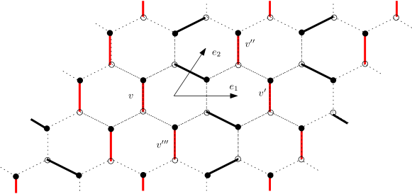
Figure 2. The graph $\Lambda_{L,N}$ with $L=5,N=4$. The graph is periodic in both $e_{1}$ and $e_{2}$ directions. Vertical dimers (in red) will be called “particles”. Here, $v^{\prime}=v+2e_{1},v^{\prime\prime}=v+e_{2}+e_{1}$ and $v^{\prime\prime\prime}=v-e_{2}+e_{1}$.

The number of dimers (i.e. of edges in the perfect matchings) equals $LN$, which is the number of white vertices. Given strictly positive integers $n_{1},n_{2}$ with $n_{1}+n_{2}<NL,$ let $\Omega_{L,N;n_{1},n_{2}}$ be the set of dimer coverings $X$ with $n_{1}$ vertical dimers and $n_{2}$ north-west oriented dimers. It is well known that the number of vertical dimers is the same in each horizontal row, so that $k_{1}:=n_{1}/N\in\mathbb{N}$, and similarly there are $k_{2}:=n_{2}/L\in\mathbb{N}$ north-west oriented dimers in each $e_{2}$-oriented column. To avoid trivialities we will also assume that $k_{1}\geq 2$ (recall that in the particle picture we required $m_{1}\geq 2$ for the same reason). Another well-known fact is that the knowledge of which vertical edges are occupied uniquely determine the whole dimer configuration. A last observation is that the horizontal (i.e. $e_{1}$) coordinates of vertical dimers are interlaced: given two vertical edges $v$ and $v^{\prime}=v+ke_{1},k>0$ such that there is a dimer at $v,v^{\prime}$ and no dimer at $v+je_{1},j=1,\dots,k-1$, then there is exactly one value $0\leq r<k$ and one value $0<s\leq k$ such that there is a dimer at $v^{\prime\prime}=v+e_{2}+re_{1}$ and at $v^{\prime\prime\prime}=v-e_{2}+se_{1}$. See Figure 2.

Remark 2.

If vertical dimers are called “particles”, then the correspondence between the particle picture of Section and the dimer picture should now be clear, see also Figure 3: for each particle configuration in $\Omega_{L,N;m_{1},m_{2}}$ there is a perfect matching of $\Lambda_{L,N}$ with certain values $(k_{1},k_{2})$, and vice-versa. It is obvious that $m_{1}=k_{1}$. It remains to be shown that also $m_{2}=k_{2}$, thereby proving also (2.1), since $Lk_{2}+Nk_{1}=n_{1}+n_{2}<NL$ by assumption. Given a nearest-neighbor path $C_{f\to f^{\prime}}$ from a face $f$ to a face $f^{\prime}$ and a perfect matching $X$, define

$$H_{X}(C_{f\to f^{\prime}})=\sum_{e\in C_{f\to f^{\prime}}}\epsilon_{e}{\bf 1}_{e\in X}$$ (2.10)

where the sum runs over the edges crossed by the path, $\epsilon_{e}$ equals $+1/-1$ if $e$ is crossed with the white vertex on the right/left and ${\bf 1}_{e\in X}$ is the indicator function that $e$ is occupied by a dimer in $X$. It is well known [11] that if $f^{\prime}=f$ then, given $X$, $H_{X}(C_{f\to f})$ depends only on the horizontal and vertical winding numbers of $C_{f\to f}$ around the torus. Choose a path $C^{(1)}_{f\to f}$ that moves only in the $+e_{1}$ direction. Then, we see that

$$H_{X}(C^{(1)}_{f\to f})=+k_{1}.$$ (2.11)

If instead $C^{(2)}_{f\to f}$ it moves only in the $+e_{2}$ direction, then

$$H_{X}(C^{(2)}_{f\to f})=-k_{2}.$$ (2.12)

On the other hand, choose $C^{(\Gamma)}_{f\to f}$ as follows: it starts from a face $f$ just to the right of a vertical dimer $p$, it moves in direction $+e_{2}$ if this involves crossing no dimer, and in the direction $+e_{1}$ otherwise; the paths stops when it gets back to $f$. Let us say that a vertical dimer $r$ “is visited by $C^{(\Gamma)}_{f\to f}$” if the path visits the hexagonal face just to the right of $r$. Note that the first visited vertical dimer is $p$, the second one is its up-right neighbor $p_{6}$, then the up-right neighbor of $p_{6}$, and so on. These are just the particles visited by the path $\Gamma$ built in Section 2.1. In particular, we have seen that $\Gamma$ forms a simple loop, so $C^{(\Gamma)}_{f\to f}$ does indeed come back to $f$. Also, $C^{(\Gamma)}_{f\to f}$ has the same winding numbers $N_{h},N_{v}$ as $\Gamma$. By construction, we see that $H_{X}(C^{(\Gamma)}_{f\to f})=0$ since the path never crosses any dimer. On the other hand, by (2.11)-(2.12) we have

$$0=H_{X}(C^{(\Gamma)}_{f\to f})=N_{h}k_{1}-N_{v}k_{2},$$ (2.13)

i.e. $k_{2}=m_{2}$, see (2.7).

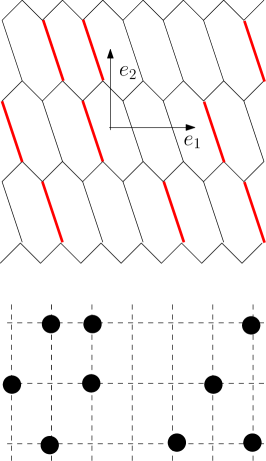
Figure 3. The correspondence between (a portion of) perfect matching and interlacing particle configuration. The mapping is made more evident by an affine deformation of the hexagonal lattice such that the axes $e_{1},e_{2}$ become orthogonal

In analogy with Section 2.1, for each vertical dimer $p$, let $p_{1},\dots p_{6}$ be the labels of its six neighboring vertical dimers labeled in clockwise order starting from the one on the right. The non-negative (possibly zero) integers $A_{p},$ $B_{p},C_{p},D_{p},E_{p},F_{p}$ defined in (2.5) are given in the coordinates of the hexagonal lattice as follows: if $p$ is at vertical edge $v$, then

$$p_{1}\text{ is at edge }v+(A_{p}+1)e_{1}; p_{2}\text{ is at edge }v-e_{2}+(B_{p}+1)e_{1}$$

$$p_{3}\text{ is at edge }v-e_{2}-C_{p}e_{1}; p_{4}\text{ is at edge }v-(D_{p}+1)e_{1}$$

$$p_{5}\text{ is at edge }v+e_{2}-(E_{p}+1)e_{1}; p_{6}\text{ is at edge }v+e_{2}+F_{p}e_{1}.$$

3. Periodized $q$-Whittaker dynamics

We saw that the descriptions in terms of interlaced particles on the torus $\mathbb{T}_{L,N}$ or of perfect matchings of $\Lambda_{L,N}$ are equivalent, if we set $(m_{1},m_{2})=(k_{1},k_{2})$. We will interchangeably use the former or the latter representation.

Definition 1.

Given a configuration $\eta\in\Omega_{L,N;m_{1},m_{2}}$, draw a directed upward edge from any particle $r$ to its up-right neighbor $r_{6}$ if $F_{r}=0$ and a downward edge from $r$ to $r_{3}$ if $C_{r}=0$ (in both cases, we draw an edge between particles in neighboring lines, with the same horizontal position). For each particle $p$ let $V^{+}_{p}$ (resp. $V^{-}_{p}$) be the set that includes $p$ plus the particles that can be reached from $p$ by following upward (resp. downward) oriented edges.

Remark 3.

From the assumption $n_{1},n_{2}>0$ it follows that $|V^{\pm}_{p}|\leq N-1$ for every $p$. In fact, if say $|V^{+}_{p}|\geq N$ then the upward edges starting from $p$ form a loop and actually $|V^{+}_{p}|=N$ (in each row there is at most one particle $p^{\prime}$ with the same horizontal position $x_{p^{\prime}}$ as $p$). In this case, the path $\Gamma$ defined just after (2.6) has zero horizontal winding number, so from (2.7) we have $m_{2}=n_{2}=0$. Therefore, the up/down arrows do not form loops and we can identify $r^{+}_{p}$, the highest particle in $V^{+}_{p}$, and $r^{-}_{p}$, the lowest particle in $V^{-}_{p}$.

The dynamics we consider is a continuous-time Markov chain on $\Omega_{L,N;m_{1},m_{2}}$. The updates consist in shifting by $+e_{1}$ all particles in one of the families $V^{+}_{p}$. Such move happens with rate

$$a_{r(p)}\,\frac{(1-q^{B_{p}})(1-q^{D_{p}+1})}{(1-q^{C_{p}+1})},$$ (3.1)

where $q\in[0,1)$ and $a_{1},\ldots,a_{N}>0$ are the same real parameters as in the definition of the Gibbs measure (2.8). Recall that $r(p)$ is the row associated to particle $p$. Note that the rate is zero if $B_{p}=0$. This prevents particles from overlapping after the move, see Figure 4 (b). Note also that after the move, the configuration is still in $\Omega_{L,N;n_{1},n_{2}}$. Indeed, if $|V_{p}^{+}|=1$, shifting $p$ by $+e_{1}$ corresponds to rotating three dimers around a hexagonal face (see Figure 4 (a)), so $n_{1},n_{2}$ remain constant. In the general case, if $B_{p}>0$ the shift of $V_{p}^{+}$ by $e_{1}$ can be obtained by shifting $+e_{1}$ the particles of $V_{p}^{+}$ one by one, starting from the top one, i.e. $r_{p}^{+}$. Also in this case, $n_{1},n_{2}$ are unchanged.

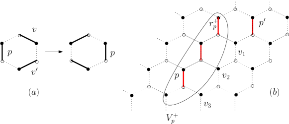
Figure 4. (a): If $|V_{p}|=1$ then necessarily edge $v$ is occupied and if $B_{p}\neq 0$ then $v^{\prime}$ is also occupied. The allowed shift of $e_{1}$ then corresponds to the rotation of these three dimers. (b): A particle $p$ with the associated set $V^{+}_{p}$, whose highest particle is $r^{+}_{p}$. The shift of $V^{+}_{p}$ by $e_{1}$ should be forbidden, otherwise particles $r^{+}_{p}$ and $p^{\prime}$ would overlap. Indeed, by the particle interlacing condition note that edges $v_{1},v_{2},v_{3}$ are necessarily occupied by particles. In particular, $B_{p}=0$ because $v_{3}$ is occupied, so that the rate (3.1) is zero.

Remark 4.

For $q=0$ and $a_{k}\equiv 1$, the dynamics was studied in [5, 6, 19] (in this case, $q^{B_{p}}$ should be interpreted as $1$ when $B_{p}=0$). As we already remarked, in this case $\pi=\pi_{L,N;m_{1},m_{2}}$ is the uniform measure over $\Omega_{L,N;m_{1},m_{2}}$. In [19], “particles” were associated to north-west oriented dimers, rather than to vertical ones as in the present work. With the convention of [19], updates consist in a single particle jumping a distance $n\geq 1$ in the $-e_{2}$ direction, instead of $n\geq 1$ particles jumping a distance $1$ in the $+e_{1}$ direction.

A preliminary observation:

Lemma 1.

The Markov chain is ergodic on $\Omega_{L,N;n_{1},n_{2}}$. More precisely, one can go from any $\eta\in\Omega_{L,N;n_{1},n_{2}}$ to any $\eta^{\prime}\in\Omega_{L,N;n_{1},n_{2}}$ via a chain of elementary moves where a single particle jumps by $+e_{1}$.

Proof of Lemma 1.

First let us define the height function $h_{\eta,\eta^{\prime}}$ of $\eta$ respective to $\eta^{\prime}$ [11]: this is defined on hexagonal faces $f$ and its gradients are given by

$$h_{\eta,\eta^{\prime}}(f^{\prime})-h_{\eta,\eta^{\prime}}(f) =H_{\eta}(C_{f\to f^{\prime}})-H_{\eta^{\prime}}(C_{f\to f^{\prime}})$$ (3.2)

$$=\sum_{v\in C_{f\to f^{\prime}}}\epsilon_{v}({\bf 1}_{v\in\eta}-{\bf 1}_{v\in\eta^{\prime}})$$

where $H_{\eta}(C_{f\to f^{\prime}})$ was defined in (2.10).

The r.h.s. of (3.2) is independent of $C_{f\to f^{\prime}}$: this amounts to the statement that $h_{\eta,\eta^{\prime}}(f^{\prime})-h_{\eta,\eta^{\prime}}(f)=0$ if $f^{\prime}=f$, which follows from the second equality in (2.13) because both $\eta,\eta^{\prime}$ are in $\Omega_{L,N;n_{1},n_{2}}$ with the same values of $n_{1}=Nk_{1},n_{2}=Lk_{2}$. The height function is therefore well-defined modulo an additive constant: let us fix this constant by establishing that $h_{\eta,\eta^{\prime}}\geq 0$ and that it vanishes at some face that we call $\bar{f}$. Given any $f$ such that $h_{\eta,\eta^{\prime}}(f)>0$, construct a path $f=f_{0},f_{1},f_{2},\dots$ with the rule that the edge traversed from $f_{i}$ to $f_{i+1}$ is not occupied in $\eta$ and has the white vertex on the left. We see then that $h_{\eta,\eta^{\prime}}$ is non-decreasing along this path. We have:

Lemma 2.

The path $f=f_{0},f_{1},f_{2},\dots$ cannot contain a closed loop.

As a consequence, it must be the case that after a finite number $k$ of steps the path cannot be continued. In this case, this implies that at face $f_{k}$ it is possible to rotate the three dimers (all three edges with white vertex on the left are occupied, as in Figure 4 (a)): the vertical one moves by $e_{1}$ and the height at $f_{k}$ decreases by $1$. Repeat the procedure until $h_{\eta,\eta^{\prime}}$ is zero everywhere.

∎

Proof of Lemma 2.

Assume by contradiction that the path contains a loop $C_{g\to g}$. We know that for every $X\in\Omega_{L,N;n_{1},n_{2}}$ we have

$$H_{X}(C_{g\to g})=H_{\eta}(C_{g\to g}).$$ (3.3)

Since all edges traversed by $C_{g\to g}$ have the white site on the left, $H_{X}(C_{g\to g})$ equals minus the number of traversed dimers. For $\eta$, we know that no dimer is traversed, so we conclude that none of the dimers traversed by $C_{g\to g}$ is occupied in any configuration $X\in\Omega_{L,N;n_{1},n_{2}}$. This leads to a contradiction with our assumption $n_{1},n_{2},NL-n_{1}-n_{2}>0$. Suppose for instance that a vertical edge is contained in no $X\in\Omega_{L,N;n_{1},n_{2}}$: by translation invariance, this would imply $n_{1}=0$. Similarly, the assumption $n_{2}>0$ and $LN-n_{1}+n_{2}>0$ exclude the case where some given non-horizontal edge is contained in none of the configurations $X\in\Omega_{L,N;n_{1},n_{2}}$. ∎

4. Invariance of Gibbs measures

Our main result is:

Theorem 1.

The probability law $\pi:=\pi_{L,N;m_{1},m_{2}}$ is stationary in time.

Remark 5.

In [19], stationarity of $\pi$ for $q=0$ and all $a_{k}\equiv 1$ was proven, and actually it was shown that the infinite volume Gibbs measures $\pi_{\rho_{1},\rho_{2}}$, obtained in the limit $L\to\infty,N\to\infty$, $m_{1}/L\to\rho_{1},m_{2}/N\to\rho_{2}$, are stationary for the dynamics on the infinite hexagonal lattice. The proof of invariance of $\pi$ on $\Lambda_{L,N}$ in the case $q>0$ is more involved than for $q=0$.

Proof of Theorem 1.

Call $\mathcal{L}$ the Markov generator, then we have to check $[\pi\mathcal{L}](\eta)=0$ for every configuration $\eta\in\Omega_{L,N;n_{1},n_{2}}$. This can be rewritten as

$$\sum_{\sigma\neq\eta}\pi(\sigma)\mathcal{L}(\sigma,\eta)+\pi(\eta)\mathcal{L}(\eta,\eta)=0.$$ (4.1)

Since the generator has sum zero on rows, this is equivalent to

$$\pi(\eta)\left[\sum_{\sigma\neq\eta}\frac{\pi(\sigma)}{\pi(\eta)}\mathcal{L}(\sigma,\eta)-\sum_{\sigma\neq\eta}\mathcal{L}(\eta,\sigma)\right]=0.$$ (4.2)

Now it is obvious from the definition of the dynamics that

$$\sum_{\sigma\neq\eta}\mathcal{L}(\eta,\sigma)=\sum_{p}a_{r(p)}\,\frac{(1-q^{B_{p}})(1-q^{D_{p}+1})}{(1-q^{C_{p}+1})}=:S_{1}(\eta).$$ (4.3)

On the other hand, we claim (see proof below) that

$$\sum_{\sigma\neq\eta}\frac{\pi(\sigma)}{\pi(\eta)}\mathcal{L}(\sigma,\eta)=\sum_{p}a_{r(p)+1}\frac{(1-q^{A_{p}+1})(1-q^{E_{p}})}{(1-q^{F_{p}+1})}=:S_{2}(\eta),$$ (4.4)

where $r(p)+1$ equals $1$ if $r(p)=N$. Finally, we claim that

$$S_{1}(\eta)=S_{2}(\eta)\quad\text{for every}\quad\eta\in\Omega_{L,N;m_{1},m_{2}}.$$ (4.5)

Proof of (4.4) An update $\sigma\to\eta$ means that a family $V^{+}_{p}$ in $\sigma$ has been shifted by $e_{1}$. Call, as in Definition 1, $r^{+}_{p}$ the highest particle in $V^{+}_{p}$. The reverse move consists in shifting $V^{-}_{r^{+}_{p}}$ by $-e_{1}$. Call $\eta_{p}$ the configuration obtained by $\eta$ by shifting $V^{-}_{p}$ by $-e_{1}$. We see then that the configurations $\eta_{p}$, with $p$ running over all particles, exhaust the configurations $\sigma$ contributing to (4.4). Next we claim that

$$\frac{\pi(\eta_{p})}{\pi(\eta)}\mathcal{L}(\eta_{p},\eta)=a_{r(p)+1}\frac{(1-q^{A_{p}+1})(1-q^{E_{p}})}{(1-q^{F_{p}+1})}.$$ (4.6)

If this is true, then (4.4) is proven. Label $p_{-\ell+1},\equiv r^{-}_{p},p_{-\ell+2},\dots,p_{0}\equiv p$ the $\ell=|V^{-}_{p}|\leq N-1$ particles that are shifted left in the move $\eta\to\eta_{p}$, starting from the lowest one. We have from (3.1),

$$\mathcal{L}(\eta_{p},\eta)=a_{r(p_{-\ell+1})}\frac{(1-q^{B_{p_{-\ell+1}}+1})(1-q^{D_{p_{-\ell+1}}})}{1-q^{C_{p_{-\ell+1}}}}.$$ (4.7)

As for the ratio of probabilities, one sees that

$$\frac{\pi(\eta_{p})}{\pi(\eta)} =\frac{a_{r(p_{0})+1}}{a_{r(p_{-\ell+1})}}\frac{(q;q)_{F_{p_{0}}}(q;q)_{C_{p_{-\ell+1}}}}{(q;q)_{F_{p_{0}}+1}(q;q)_{C_{p_{-\ell+1}}-1}}$$ (4.8)

$$\,\,\,\,\,\times\prod_{j=-\ell+1}^{0}\frac{(q;q)_{A_{p_{j}}+1}(q;q)_{D_{p_{j}}-1}}{(q;q)_{A_{p_{j}}}(q;q)_{D_{p_{j}}}}\frac{(q;q)_{E_{p_{j}}}(q;q)_{B_{p_{j}}}}{(q;q)_{E_{p_{j}}-1}(q;q)_{B_{p_{j}}+1}}$$

$$=\frac{a_{r(p_{0})+1}}{a_{r(p_{-\ell+1})}}\frac{(1-q^{C_{p_{-\ell+1}}})}{(1-q^{F_{p_{0}}+1})}\prod_{j=-\ell+1}^{0}\frac{(1-q^{A_{p_{j}}+1})(1-q^{E_{p_{j}}})}{(1-q^{D_{p_{j}}})(1-q^{B_{p_{j}}+1})}.$$

Note that the $F$’s and $C$’s of intermediate particles do not appear because they are exactly zero, both in $\eta$ and in $\eta_{p}$. Also, note that $B_{p_{0}}=A_{p_{1}},\dots,B_{p_{-\ell+2}}=A_{p_{-\ell+1}}$ and $E_{p_{-1}}=D_{p_{0}},\dots,E_{p_{-\ell+1}}=D_{p_{-\ell+2}}$. Therefore, (4.8) simplifies into

$$\frac{a_{r(p_{0})+1}}{a_{r(p_{-\ell+1})}}\,\frac{(1-q^{C_{p_{-\ell+1}}})(1-q^{A_{p_{0}}+1})(1-q^{E_{p_{0}}})}{(1-q^{B_{p_{-\ell+1}}+1})(1-q^{D_{p_{-\ell+1}}})(1-q^{F_{p_{0}}+1})}.$$ (4.9)

Once we multiply (4.7) by (4.9) and we recall that $p_{0}=p$, we obtain (4.6) and therefore (4.4). ∎

Proof of (4.5).

It is sufficient to prove that $S_{1}-S_{2}$ is independent of $\eta$. In this case, it must be zero because $\sum_{\eta}[\pi\mathcal{L}](\eta)=0$ by conservation of the probability. Thanks to Lemma 1 it is sufficient to show that $S_{1}-S_{2}$ is unchanged when a single particle is moved by $e_{1}$. The sums in $S_{1},S_{2}$ make sense also when horizontal particle positions are real numbers; given a particle $p$ that can be moved by $e_{1}$, we let $\eta(s)$ be the configuration where $p$ is moved by $se_{1},s\in[0,1]$ and we prove that $\partial_{s}(S_{1}-S_{2})=0$. Note that not only the values of $A_{p},\dots,F_{p}$ depend on $s$, but also $D_{p_{1}},E_{p_{2}},F_{p_{3}},A_{p_{4}},B_{p_{5}},C_{p_{6}}$ do. We find by direct computation

$$\frac{\partial_{s}S_{1}}{\log q}=a_{r(p)}S_{10}+a_{r(p)+1}S_{11},\quad\text{and}\quad\frac{\partial_{s}S_{2}}{\log q}=a_{r(p)}S_{20}+a_{r(p)+1}S_{21},$$ (4.10)

where

$$S_{10} =q^{B_{p}}\frac{1-q^{D_{p}+1}}{1-q^{C_{p}+1}}-q^{D_{p}+1}\frac{1-q^{B_{p}}}{1-q^{C_{p}+1}}$$ (4.11)

$$\,\,\,\,\,+q^{C_{p}+1}\frac{(1-q^{B_{p}})(1-q^{D_{p}+1})}{(1-q^{C_{p}+1})^{2}}+q^{D_{p_{1}}+1}\frac{1-q^{B_{p_{1}}}}{1-q^{C_{p_{1}}+1}},$$

$$S_{11} =-q^{C_{p_{6}}+1}\frac{(1-q^{D_{p_{6}}+1})(1-q^{B_{p_{6}}})}{(1-q^{C_{p_{6}}+1})^{2}}-q^{B_{p_{5}}}\frac{1-q^{D_{p_{5}}+1}}{1-q^{C_{p_{5}}+1}},$$ (4.12)

$$S_{20} =q^{F_{p_{3}}+1}\frac{(1-q^{A_{p_{3}}+1})(1-q^{E_{p_{3}}})}{(1-q^{F_{p_{3}}+1})^{2}}+q^{E_{p_{2}}}\frac{1-q^{A_{p_{2}}+1}}{1-q^{F_{p_{2}}+1}},$$ (4.13)

$$S_{21} =q^{A_{p}+1}\frac{1-q^{E_{p}}}{1-q^{F_{p}+1}}-q^{E_{p}}\frac{1-q^{A_{p}+1}}{1-q^{F_{p}+1}}$$ (4.14)

$$\,\,\,\,\,-q^{F_{p}+1}\frac{(1-q^{A_{p}+1})(1-q^{E_{p}})}{(1-q^{F_{p}+1})^{2}}-q^{A_{p_{4}}+1}\frac{1-q^{E_{p_{4}}}}{1-q^{F_{p_{4}}+1}}.$$

Using $D_{p_{1}}=A_{p},C_{p_{1}}=A_{p}-B_{b},C_{p_{6}}=F_{p},D_{p_{6}}=E_{p}+F_{p},B_{p_{6}}=A_{p}-F_{p},B_{p_{5}}=E_{p},C_{p_{5}}=D_{p}-E_{p}$ we get

$$S_{10} =q^{B_{p}}\frac{1-q^{D_{p}+1}}{1-q^{C_{p}+1}}-q^{D_{p}+1}\frac{1-q^{B_{p}}}{1-q^{C_{p}+1}}$$ (4.15)

$$\,\,\,\,\,+q^{C_{p}+1}\frac{(1-q^{B_{p}})(1-q^{D_{p}+1})}{(1-q^{C_{p}+1})^{2}}+q^{A_{p}+1}\frac{1-q^{B_{p_{1}}}}{1-q^{A_{p}-B_{p}+1}}$$

$$S_{11} =-q^{F_{p}+1}\frac{(1-q^{F_{p}+E_{p}+1})(1-q^{A_{p}-F_{p}})}{(1-q^{F_{p}+1})^{2}}-q^{E_{p}}\frac{1-q^{D_{p_{5}}+1}}{1-q^{D_{p}-E_{p}+1}}$$ (4.16)

while using $A_{p_{4}}=D_{p},E_{p_{4}}=E_{p}+D_{p_{5}}-D_{p},F_{p_{4}}=D_{p}-E_{p},F_{p_{3}}=C_{p},A_{p_{3}}=B_{p}+C_{p},E_{p_{3}}=D_{p}-C_{p},A_{p_{2}}=A_{p}+B_{p_{1}}-B_{p},E_{p_{2}}=B_{p},F_{p_{2}}=A_{p}-B_{p},$

$$S_{20} =q^{C_{p}+1}\frac{(1-q^{B_{p}+C_{p}+1})(1-q^{D_{p}-C_{p}})}{(1-q^{C_{p}+1})^{2}}+q^{B_{p}}\frac{1-q^{A_{p}+B_{p_{1}}-B_{p}+1}}{1-q^{A_{p}-B_{p}+1}}$$ (4.17)

$$S_{21} =q^{A_{p}+1}\frac{1-q^{E_{p}}}{1-q^{F_{p}+1}}-q^{E_{p}}\frac{1-q^{A_{p}+1}}{1-q^{F_{p}+1}}$$ (4.18)

$$\,\,\,\,\,-q^{F_{p}+1}\frac{(1-q^{A_{p}+1})(1-q^{E_{p}})}{(1-q^{F_{p}+1})^{2}}-q^{D_{p}+1}\frac{1-q^{E_{p}+D_{p_{5}}-D_{p}}}{1-q^{D_{p}-E_{p}+1}}$$

Note that, when taking the difference $S_{10}-S_{20}$, the dependence on $B_{p_{1}}$ cancels and likewise for the difference $S_{11}-S_{21}$ the dependence on $D_{p_{5}}$ cancels. Finally, one checks that each of these differences, which a priori depends on $q,A_{p},\dots,F_{p}$, is actually identically zero and (4.5) is proven. This concludes the proof of Theorem 1. ∎

References

- [1] E. Andjel, Invariant measures for the zero range process Ann. Probab. 10 (1982), 525–547.
- [2] G. Barraquand, I. Corwin, Random-walk in Beta-distributed random environment, arXiv:1503.04117.
- [3] A. Borodin, On a family of symmetric rational functions, arXiv:1410.0976.
- [4] A. Borodin, A. Bufetov, An irreversible local Markov chain that preserves the six vertex model on a torus, in preparation.
- [5] A. Borodin, P. L. Ferrari, Anisotropic KPZ growth in dimensions, Comm. Math. Phys. 325 (2014), 603–684.
- [6] A. Borodin, P. L. Ferrari, Anisotropic KPZ growth in dimensions: fluctuations and covariance structure, J. Stat. Mech. (2009), P02009.
- [7] A. Borodin, I. Corwin, Macdonald processes, Probab. Theory Relat. Fields 158 (2014), 225–400.
- [8] A. Borodin, L. Petrov, Nearest neighbor Markov dynamics on Macdonald processes, arXiv:1305.5501.
- [9] M. Evans, S. Majumdar, R. Zia, Construction of the factorized steady state distribution in modesl of mass transport, J. Stat. Mech. (2004).
- [10] D. J. Gates, M. Westcott, Stationary states of crystal growth in three dimensions, J. Stat. Phys. 81 (1995), 681–715.
- [11] R. Kenyon, Lectures on Dimers, arXiv:0910.3129.
- [12] R. Kenyon, A. Okounkov, S. Sheffield, Dimers and amoebae, Ann. Math. 163 (2006), 1019–1056.
- [13] N. O’Connell, M. Yor, Brownian analogues of Burke’s theorem, Stoch. Proc. Appl. 96 (2001), 285–304.
- [14] M. Prähofer, H. Spohn, An exactly solved model of three dimensional surface growth in the anisotropic KPZ regime, J. Stat. Phys. 88 (1997), 999–1012.
- [15] J. Quastel, B. Valko, Diffusivity of lattice gases, Arch. Rat. Mech. Anal. 210 (2013), 269–320.
- [16] T. Sasamoto, H. Spohn, Superdiffusivity of the 1D lattice Kardar-Parisi-Zhang equation, J. Stat. Phys. 137 (2009), 917–935.
- [17] T. Seppäläinen, Scaling for a one-dimensional directed polymer with boundary conditions, Ann. Probab. 40 (2012), 19–73.
- [18] F. Spitzer, Interaction of Markov processes, Adv. Math. 5 (1970), 246–290.
- [19] F. L. Toninelli, A -dimensional growth process with explicit stationary measures, arXiv:1503.05339.