Object Recognition from Short Videos for Robotic Perception
Abstract
Deep neural networks have become the primary learning technique for object recognition. Videos, unlike still images, are temporally coherent which makes the application of deep networks non-trivial. Here, we investigate how motion can aid object recognition in short videos. Our approach is based on Long Short-Term Memory (LSTM) deep networks. Unlike previous applications of LSTMs, we implement each gate as a convolution. We show that convolutional-based LSTM models are capable of learning motion dependencies and are able to improve the recognition accuracy when more frames in a sequence are available. We evaluate our approach on the Washington RGBD Object dataset and on the Washington RGBD Scenes dataset. Our approach outperforms deep nets applied to still images and sets a new state-of-the-art in this domain.
I INTRODUCTION
Deep neural networks (DNNs) have been established as a predominant method for object recognition. By taking advantage of large datasets and learning capacity, deep networks are able learn to recognize many object categories. Generalizing deep networks to work on videos is a hard problem since video frames are highly correlated. Here, we study the problem of object recognition from short videos (up to 5 frames). This is a common scenario in robotics perception, for example, a camera-mounted robotic arm manipulator can record a small video as it approaches an object, and use it for better recognition. Similarly, when data is acquired by a mobile phone, a short video sequence can be taken instead of still image for better recognition. We argue that the motion, readily available in the videos, should be used as an additional cue for recognition and present a method capable of taking advantage of it. Our method is based on recurrent convolutional neural network where we use convolutional Long Short-Term Memory (LSTM) layer to capture motion information.
We summarize our contributions as follows:
-
•
Introduce a fast baseline DNN network which achieves accuracy competitive with the state-of-the-art on the Washinton-RGBD Object dataset, while running at 0.1 seconds per image on GPU and without using segmentation masks.
-
•
Present a motion model, based on LSTM, which uses convolution at each of its gates, and show that it is advantageous for recognition and can generalize to more frames. The model uses fewer parameters than the baseline and runs at 0.87 seconds per two frame sequences, which makes it practically relevant. To our knowledge this is the first application of fully-convolutional LSTM networks.
-
•
Experiment extensively on Washington-Object and Washington-Scenes datasets and set a new state-of-the-art in the domain on both datasets.
II Previous work
Object recognition for robotics applications has been of interest for a number of years [1] with more advanced and sophisticated algorithms [2, 3] making their way into this application domain [4, 5, 6]. Deep neural networks have also recently been applied to the problems, such as object recognition and grasp detection, and demonstrated advancements [7, 8].
LSTMs have been introduced by Hochreiter and Schmidhuber with their pioneering work in [9]. A. Graves and collaborators [10, 11] further developed LSTMs and showed important improvements and practical applications to various domains with sequence data-processing, such as handwriting recognition [10, 12] and speech recognition [13, 11]. Recurrent neural networks have also recently been successfully applied for phoneme recognition [14], translation [15] or for generating text descriptions of input images [16].
In video analysis, several applications of RNNs or LSTMs have been proposed for improving recognition from consecutive image frames. For example, Karpathy et al. [17] applied a 3D convolutions for classification of sports videos, and Ng et al. [18] applied a combination of LSTMs and global pooling techniques for classification of sports videos, or other action recognition videos. The key difference with our work is that instead of LSTM, based on fully connected gates, we use convolutional-only LSTM gates which allow us to model local motion deformations. Additionally, other approaches are typically applied for long video sequences. Because of high computational cost, they have to be applied offline and can afford much larger and slower LSTM architectures, or may choose to combine LSTM-based methods with optical flow, or others techniques [18]. We, on the other hand, focus on object recognition from small sequences of image frames, e.g. taken within one second, which is relevant to robotics perception or mobile phone recognition.
III Approach
III-A Baseline convolutional neural network
Since winning ImageNet challenge for image recognition [19], convolutional neural networks (CNNs) have become widely used in object recognition. By stacking multiple layers on top of each other, CNNs can learn progressively higher level representations of the images thus performing feature learning. For image-based inputs, the first layers are typically convolutional, targeted at learning local visual features, whereas the subsequent layers are fully-connected.
We first build a baseline CNN architecture for object recognition for a single frame. Inspired by [19], we build our baseline model using three convolutional layers, followed by two fully connected layers with dropouts. We note that unlike [19], our network has been designed to be very small (fewer and smaller convolutional filters), and thus is very fast at inference. The supplementary material provides details of the architecture of this network and visualizes it.
III-B Long Short-Term memory
Recurrent neural networks (RNNs) represent a more general class of networks, where connections from hidden units can be used as input to the network [9, 10]. Because of recurrent connections, RNNs are capable of learning dynamic relationship in the data. One of drawbacks of RNNs is that during training, which is done by backpropagation, the gradient may either become very small or too large, problems known as “vanishing gradient” and “exploding gradient”, respectively. To solve this problem, Long Short-Term Memory (LSTM) [20] introduced special memory cells to store information for multiple time steps. LSTM architecture is a block consisting of an input gate, a neuron which has a recurrent connection, a forget gate and an output gate. The motivation behind such blocks is to allow the network to read (input gate), write (output gate) and reset (forget gate), similar to operations available to a digital computer. Formally, the transformation taking place in an LSTM layer is as follows: let be an input sequence where is a timestep. The input gate, , and an internal gate which is a candidate to be placed into a memory block, , are:
| (1) |
| (2) |
where is the LSTM output at timestep and are the weight matrices and biases for the input gate and the memory block, and is the sigmoid function. Note that all gates are a function of the input at a current time step, , and the output of previous step, , forming recurrent dependency. In the original LSTM design [20], the content of the memory cell at the time step is a linear combination of the current memory cell candidate and the content of the cell’s memory at previous time step:
| (3) |
where is the element-wise addition operation. This could lead to unbounded values of the memory cell. A solution is to reset some of the elements of the previous memory cell with the aid of the forget gate [21]. Empirically it was found that the forget gate plays a crucial role in the LSTM design and removing it decreases performance [22]. The forget gate, and the memory state, are computed as follows:
| (4) |
| (5) |
The forget gate serves as a way to reset activations from previous memory cell which might not be as important at the current time step. Note that all this behavior is learned via the weights of the LSTM and is thus adapted to the data observed. The final output is given as a function of the output gate multiplied by the activation of the memory cell at the current time step:
| (6) |
| (7) |
Because of memory cells, LSTM can transfer information across different timesteps, an essential feature if we are to use dynamics of the input to aid recognition.
III-C Convolutional LSTM for modeling motion
Not all motion information in sequences of frames is useful when recognizing objects. For example, camera motion or the motion of the environment (e.g., turning motion of the turntable with the object of the interest) is not relevant to the identity of the object. Thus, the neural network’s architecture has to be designed in a way as to account for the situation in which the relevant motion is local. For example, when a cup rotates on a turntable, only the shape of the handle deforms, while the overall shape of the cup remains the same. To extract such local motion information, we propose to implement the LSTM module in terms of convolutions, instead of fully connected layers, as was previously done. Since each gate in the LSTM is convolutional, the recurrent network is capable to act upon local motion from the video which is specific to each object. Another benefit of convolutional-only based LSTM is that it requires significantly fewer parameters, compared to a fully connected LSTM. This allows to reduce overfitting, and generalizes better, which is particularly important especially when the training data is limited. Our experiments, presented later in the paper, further validate that the proposed fully-convolutional LSTM is a much better architecture in terms of accuracy for this task, compared to other alternatives.
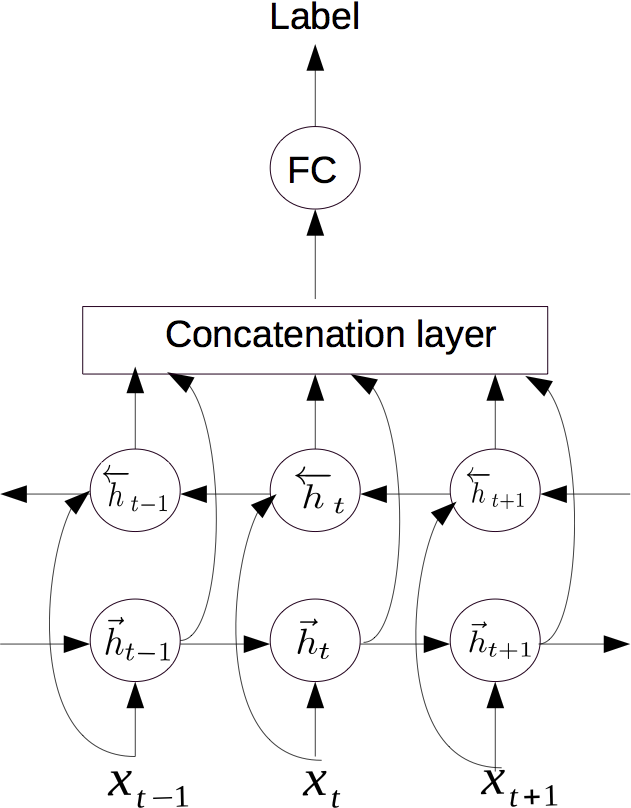
III-D Bidirectional LSTM
The LSTM architecture, presented in Sec. III-B, allows dynamic information to pass only in one direction, i.e. for timesteps , such that , the output of has access to the information available at previous timestep , but does not have access to . A bidirectional LSTM architecture was proposed [23] to overcome this. In bidirectional LSTM, the input sequence is passed into two separate LSTM layers in forward and reverse directions. In Sec. IV-A5 we further explore how presenting the input sequences in one or both directions affect the network’s learning capabilities.
III-E Motion model for image sequences
This section summarizes the architecture of our proposed convolutional LSTM-based motion model.
The first three layers in our LSTM-based motion model are convolutional layers, as in the baseline (Section IV-C1 provides specific details of their parameters). This is done to allow the network to learn low-level features. These layers are followed by bidirectional LSTM modules with convolutional gates. Each gate of the LSTM is implemented as a convolutional layer with stride 1, filter size 5 and depth 256. The hidden layers from the forward and backward LSTM are concatenated and fed into a fully connected layer followed by a softmax layer. The network architecture is shown in Fig. 1 and is visualized in more detail in the supplementary material. For 4-frame sequence our motion model uses 66 million parameters whereas the baseline uses 77 million. As previously mentioned, the convolutional-only and the bidirectional design is proposed to address the problem of learning from short video sequences.
IV Experimental evaluation
We evaluated our method on publicly available datasets and compared it to the state-of-the-art. First, we tested on Washington RGBD Object dataset [3], which has been the most common to test object recognition for robotic perception. Although Washington RGBD Object dataset is one of the largest and most popular, it was recorded in a controlled environment. To evaluate our method in more realistic settings, we used the Washington Scenes dataset111https://goo.gl/wOAsla [3]. The Scenes dataset contains videos recorded in settings, such as a kitchen or an office, with multiple objects occurring naturally.
IV-A Washington Object dataset results
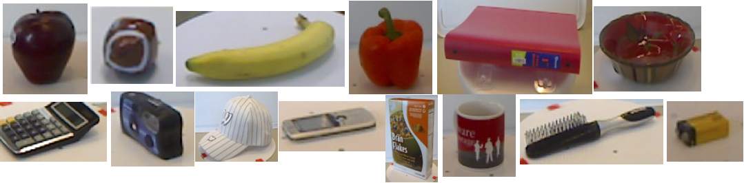
The Washington Object dataset [3] is a collection of images of objects from different categories. The dataset was collected by taking images of the objects located on a turntable from 3 different viewing angles. The dataset contains around 250,000 images from objects such as flashlight, cup, ball, apple and others. From all the images only every fifth frame is used for training or testing. Fig. 2 contains a sample set of classes in the dataset. The standard evaluation protocol [3] uses cross-validation splits when reporting results, which we also follow in this paper. It is worth noting that the dataset contains extra information e.g. segmentation masks and depth images which are not used in our experiments neither for training nor for testing.
IV-A1 Summary of results
Table I shows the results of our algorithm on the Washington Object dataset. We present the results of our baseline (Section IV-A2) and of our motion model (Section III-E). Our motion model is tested in two scenarios: natural (or “short-time frame”) and “wide viewpoint” settings, and for different number of frames. In the natural setting, the sequences we used are taken less then a second apart - a common scenario when using mobile device to take a picture of an object in the real world. In the second scenario the images of the objects are taken as far apart as possible as to maximize the viewpoints of the object.
From our results with motion from short video sequences, we can see that the motion models, in all settings, outperform previous strong baselines on still images. This indicates that motion can be used to enhance performance and with it, a new state-of-the-art for RGB input can be established. On the wide viewpoint dataset, the motion model outperforms all prior state-of-the-art results and shows a clear pattern of generalization when presented with longer sequences. Additionally, we also compare to a motion-based baseline which uses the same video sequences but does not apply convolutional LSTM. This method, also shows benefits of the motion information; it can be practically utilized to solve the same problem with somewhat inferior performance to an LSTM-based model. The sections below provide details of these experiments.
IV-A2 Baseline
Our baseline model (Section III-E) achieves an accuracy of which makes it comparable to the state of the art on the dataset. The method [7] uses additional segmentation masks and has a better overall performance at . It is worth noting that our baseline model is pretty fast as it takes second per image to perform recognition.
| Model | Accuracy | Standard Deviation |
|---|---|---|
| Single frame dataset. | ||
| Lai et. al. [3] | 74.3 | 3.3 |
| Bosch et. al. [24] | 80.2 | 1.8 |
| Socher et. al. [25] | 80.8 | 4.2 |
| Bo et. al. [2] | 82.4 | 3.1 |
| Schwarz et. al. [7] | 83.1 | 2 |
| Ours: baseline | 82.02 | 1.96 |
| Short time-frame sequence dataset | ||
| Motion model | 82.74 | 1.76 |
| Baseline + multi-frame average pooling during test | 82.66 | 1.8 |
| Wide viewpoint: frame dataset | ||
| Motion model | 83.32 | 1.96 |
| Baseline + multi-frame average pooling during test | 83.07 | 1.8 |
| Wide viewpoint: frame dataset | ||
| Motion model | 84.29 | 2 |
| Baseline + multi-frame average pooling during test | 82.45 | 1.9 |
| Wide viewpoint: frame dataset | ||
| Motion model | 84.23 | 1.84 |
| Baseline + multi-frame average pooling during test | 84.18 | 1.67 |
IV-A3 Motion model analysis
We analyze our architecture by exploring different model variations. The original LSTM, as applied to speech processing, is based on fully connected layers [11, 13, 14]. In videos, such LSTM with fully connected layers, applied after a feature extraction phase (after the first convolutional layers), would allow to model global motion of the object. We conjecture that in our application, an LSTM with convolutions would allow to model local deformations of the object caused by the motion. We experimented with different LSTM architectures by varying the parameters of convolutional-based LSTM and/or adding fully-connected layers to a fully-connected LSTM. Table II compares the different architectures.
| Model | Accuracy | Standard Deviation |
|---|---|---|
| Single frame dataset. | ||
| Baseline model trained on single image. 3 conv + 3 pools FC dropout FC dropout | 82.02 | 1.96 |
| Short time-frame sequence dataset | ||
| 3 conv + 3 pools with 128-dim FC LSTM | 75 | 3.14 |
| 3 conv + 3 pools 512-dim FC 128-dim FC LSTM | 79.27 | 3.3 |
| 3 conv + 3 pools conv LSTM (filter size = 3, depth = 128) | 81.12 | 1.75 |
| 3 conv + 3 pools conv LSTM (filter size = 5, depth = 256) where result of LSTM layers is summed | 82.24 | 2.49 |
| 3 conv + 3 pools conv LSTM (filter size = 5, depth = 256) where result of LSTM layers is concatenated | 82.59 | 1.78 |
In these experiments we use sequences which are more realistic i.e. obtained in less than a second apart. Thus, the dataset was created by mapping frame to a sequence and is referred to as “short time-frame”, Fig. 3. Such mapping allows frames to be distinct enough to contain useful motion information, but not too far apart as to be useful in a real world application (two frames in less than a second apart).
The results in Table II suggest that LSTMs implemented as fully-connected layers do not perform well and have high deviation. This might be due to overfitting since the model can learn non-existing global patterns which are irrelevant to the object’s identity. The architectures based on convolutional LSTM gates perform significantly better and also have lower standard deviation. Increasing the filter size of convolution and increasing the depth of the channels improves the performance, as well. Although increasing filter size and depth significantly increases the computational cost, our best motion model runs at 0.8 seconds per two-frame sequence, which is 4 times faster than the multi-frame baseline when averaged per image. We also experimented by stacking multiple LSTM layers one of top of each other, but the accuracy was significantly lower than the models presented in this section. We note that the results summarized in Table I (including for short-time frame sequences) are obtained by bidirectional testing, whereas Table II reports the unidirectional counterparts.
IV-A4 Wide viewpoint sequences
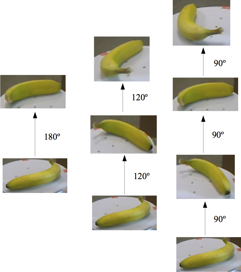
To see if our best motion model is capable of generalizing to more frames we created wide viewpoint sequence datasets. Such sequences were created to take advantage of varying viewpoints of the objects. The data was generated by taking frames to form a sequence if they are as far apart as possible in terms of viewing angle. For example, for a sequence of two frames consists of the original first frame and the frame which corresponds to the one where the object is rotated at 180 degrees. Similarly, when we create a sequence of frames which have the object rotated at degrees. An example of wide viewpoint sequence of banana for is given in Fig. 4.
Table I shows the results of the motion model which was applied to wide viewpoint datasets. We can observe that using motion models is beneficial, even for as few as one additional frame (2-frame model). Furthermore, we see that adding more frames improves performance, but for the wide-viewpont model the accuracy levels off at 4 frames. This is as expected since all viewpoints are sampled on a sphere and at some point sampled frames would coincide with existing one in the training set, thus not adding any additional information.
IV-A5 Bidirectional models
Bidirectional LSTM models [26], where there is LSTM layer for sequence in each of the directions, was found to be superior to unidirectional models [26, 14, 23]. We found that such models are indeed superior for the classification task from videos. Videos, unlike audio signals, are semantically sound regardless of the direction they are played e.g. the video played backwards can still convey the same meaning. Thus, we opt to investigate if it is possible to take advantage of this property at the data level. To do so we trained our model using dataset where sequences were passed in both directions during training and/or testing. During training this effectively doubles the size of the dataset while for testing we classify a sequence in each of the directions and average the result.
| Model | Accuracy | Standard Deviation |
|---|---|---|
| Short time-frame sequence dataset. | ||
| Unidirectional train and test | 82.59 | 1.78 |
| Bidirectional training / unidirectional testing | 82.61 | 2.29 |
| Bidirectional training and testing | 82.68 | 2.27 |
| Bidirectional testing / unidirectional training | 82.74 | 1.76 |
Results in Table III suggest that bidirectional training has almost no effect besides increasing the deviation. This result goes in hand with the architecture of the network - bidirectional LSTM allows to pass information in both directions, thus explicitly training it in this way is redundant. Although bidirectional test is worse for 2-frame wide viewpoint dataset it increases the accuracy for every other experiment.
On wide viewpoints datasets bidirectional testing showed a rather significant improvement over unidirectional one. For 3-frame dataset the accuracy increased from by more than to while for -frame dataset the increase was . On 2-frame datasets such strategy improved the accuracy on short time sequence dataset by , but decreased it for wide viewpoint one by .
IV-A6 Pooling baseline
We also compared to the baseline which uses all frames from the sequences available during training. When given a sequence of frames during testing our baseline model would take an average of the class probability distribution across all frames in a sequence. We also experimented by taking the maximum instead of multi-frame average pooling, but the accuracy was always lower.
IV-B Evaluation on Washington Scenes dataset
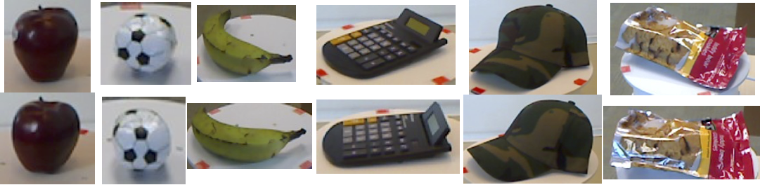
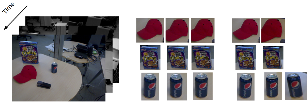
To see how well our method works on more realistic videos we performed experiments on Washington Scenes dataset [3] (see Fig. 5). The dataset consists of five videos of the office containing the following objects: soda can, bowl, cap, coffee mug, cereal box and flashlight. We cropped objects throughout videos and used one independent video “table_small” for testing and the rest for training. Because the test set did not contain a single image of the flashlight we removed the first 200 frames of the flashlight and added them to the test set, without any overlap. We evaluated our model by taking 1, 3, 5, and 10 prior frames to form sequences. For example, for 10 and for a 3-frame sequence, we compose a sequence of frames . If the frames did not exist or the objects were not visible at a particular frame, the original crop was used instead, although other solutions are also possible. Fig. 6 contains an example of a video frame and related object crops.
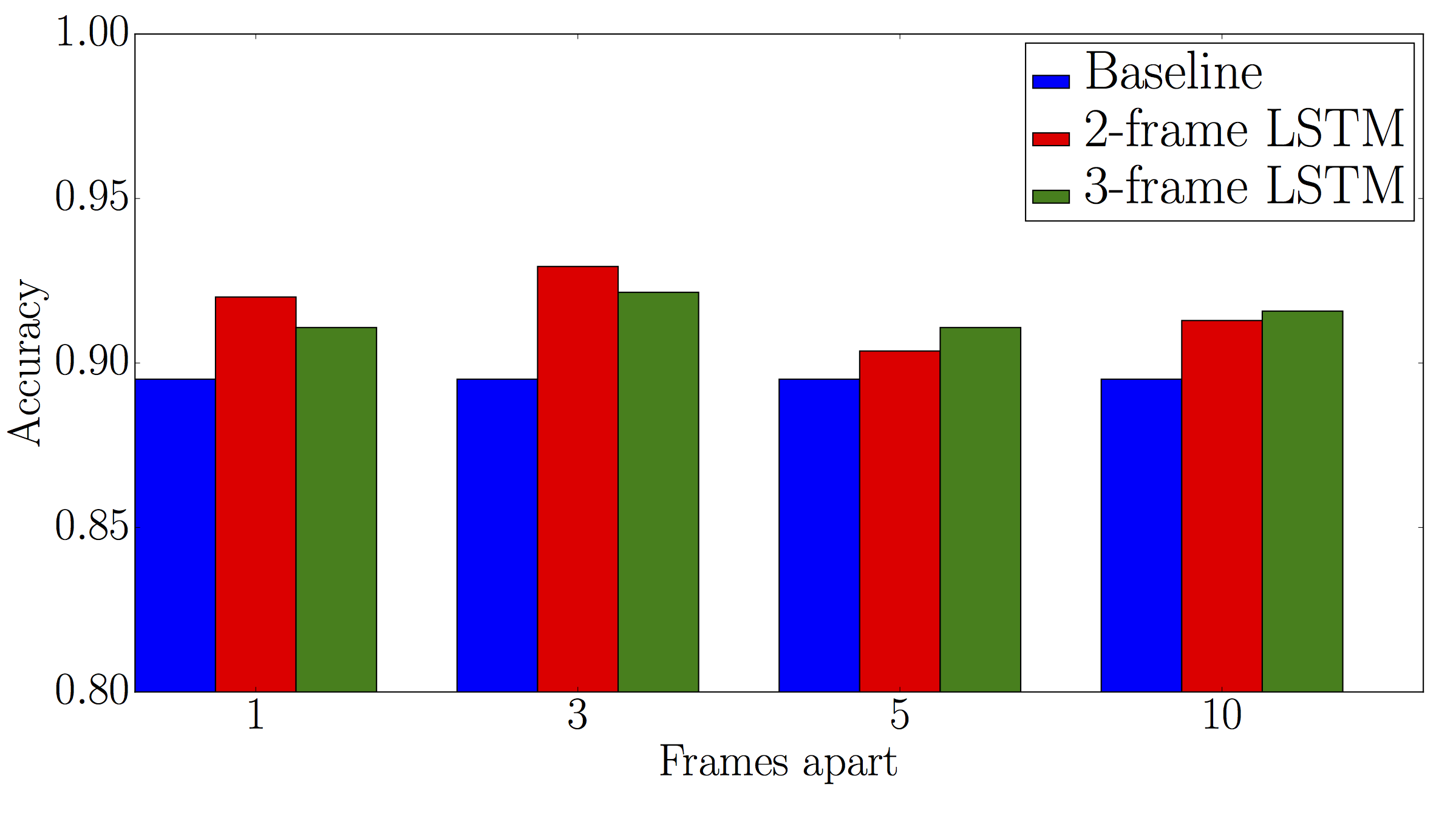
Results are reported in Fig. 6. These experiments also confirm that our motion model is beneficial as it is capable of using motion information from sequences. As images in sequences become more far apart, from 1 to 3 frames, our motion model improves as the latter sequences contain more motion information. We note that for this dataset, we have used the same network architecture and learning hyper-parameters as for Washington Object dataset, so these results are an indicator of the universality and the generalization capabilities of our proposed model. It can also be seen from Fig. 6, that the accuracies decrease for 5 and 10 frame dataset a bit probably due to bad quality of the data, which is due to the fact that the object goes out-of-view in the original scene videos: more than 50 % and 80 % of sequences, respectively, had to use shorter sequences, as the object was not visible (i.e. the corresponding frames were missing). Thus we observe, that in practical applications, learning needs to be done from frames that are not too far apart; although in principle multiple frames are capable of providing extra information, in practice, these frames may often not be available and thus are not useful. This also enforces our view that learning from short videos is the most cost-effective for object perception.
IV-C Implementation details
IV-C1 Baseline model parameters
The convolutional layers parameters are: stride 2, filter size 5, depth 64 for the first convolutional layer; stride 1, filter size 3, depth 128 for the second and the third. Each pooling layer has a stride of 2 in and direction. Each of the fully connected layers has a dimension of 4096; dropout probability is set to 0.5. In total, our baseline model has 77 million parameters.
IV-C2 Initialization
Deep CNNs allow to train powerful classifiers, but require significant amount of data to do so. To overcome this, CNNs are often initialized from networks trained on large datasets like ImageNet[27], e.g. [28]. In all of our models we initialize the first three convolutional layers by pre-training a network, as in [19], on ImageNet.
IV-C3 Learning rates
All models using baseline architecture were trained with the learning rate of . For motion models we used .
IV-C4 Runtime
We timed our models to see how fast can they perform recognition. Baseline model: 0.1 s/image; two-frame motion model: 0.87 s/image. The timings are reported using single NVidia K40 GPU.
V Conclusion
This paper proposes using motion information to improve object recognition for robotics perception. Here we used motion information from very short video sequences (e.g. 2-4 frames) to improve object recognition. We designed a recurrent neural network, based on convolutional-only LSTM, capable of utilizing motion information to guide the recognition task. We showed that bidirectional LSTM with unidirectional training and bidirectional testing is the best model for this purpose. Our experiments on wide viewpoint and natural videos showed that such motion model is capable of generalizing when more frames are available and is able to outperform baseline non-recurrent convolutional network.
VI Acknowledgements
The authors would like to thank Alex Krizhevsky for his help and comments, and the Google Brain team for providing inspiring environment and computational resources to carry out experiments.
References
- [1] S. Gould, P. Baumstarck, M. Quigley, A. Y. Ng, and D. Koller, “Integrating visual and range data for robotic object detection,” in Workshop on Multi-camera and Multi-modal Sensor Fusion Algorithms and Applications-M2SFA2 2008, 2008.
- [2] L. Bo, X. Ren, and D. Fox, “Unsupervised feature learning for rgb-d based object recognition,” in Experimental Robotics. Springer, 2013, pp. 387–402.
- [3] K. Lai, L. Bo, X. Ren, and D. Fox, “A large-scale hierarchical multi-view rgb-d object dataset.” IEEE, 2011, pp. 1817–1824.
- [4] Z. Jia, A. Saxena, and T. Chen, “Robotic object detection: Learning to improve the classifiers using sparse graphs for path planning,” in IJCAI Proceedings-International Joint Conference on Artificial Intelligence, vol. 22, no. 3, 2011, p. 2072.
- [5] A. Collet, D. Berenson, S. S. Srinivasa, and D. Ferguson, “Object recognition and full pose registration from a single image for robotic manipulation,” in Robotics and Automation, 2009. ICRA’09. IEEE International Conference on. IEEE, 2009, pp. 48–55.
- [6] S. Pillai and J. Leonard, “Monocular slam supported object recognition,” arXiv preprint arXiv:1506.01732, 2015.
- [7] M. Shwarz, H. Shulz, and S. Behnke, “Rgb-d object recognition and pose estimation based on pre-trained convolutional neural network features.” IEEE, 2015.
- [8] I. Lenz, H. Lee, and A. Saxena, “Deep learning for detecting robotic grasps,” The International Journal of Robotics Research, vol. 34, no. 4-5, pp. 705–724, 2015.
- [9] S. Hochreiter and J. Schmidhuber, “Long short-term memory,” Neural Computing, 1997.
- [10] A. Graves, A.-R. Mohamed, and G. E. Hinton, “Offline handwriting recognition with multidimensional recurrent neural networks,” NIPS, 2008.
- [11] A. Graves and N. Jaitly, “Towards end-to-end speech recognition with recurrent neural networks,” ICML, 2014.
- [12] A. Graves, M. Liwicki, S. Fernandez, H. B. R. Bertolami, and J. Schmidhuber, “A novel connectionist system for unconstrained handwriting recognition,” IEEE Trans. PAMI, 2009.
- [13] A. Graves, A.-R. Mohamed, and G. E. Hinton, “Speech recognition with deep recurrent neural networks,” CoRR, abs/1303.5778, 2013.
- [14] S. Fernandez, A. Graves, and J. Schmidhuber, “Phoneme recognition in timit with blstm-ctc,” CoRR, abs/0804.3269, 2008.
- [15] I. Sutskever, O. Vinyals, and Q. V. Le, “Sequence to sequence learning with neural networks,” in Advances in neural information processing systems, 2014, pp. 3104–3112.
- [16] O. Vinyals, A. Toshev, S. Bengio, and D. Erhan, “Show and tell: A neural image caption generator,” arXiv preprint arXiv:1411.4555, 2014.
- [17] A. Karpathy, G. Toderici, S. Shetty, T. Leung, R. Sukthankar, and L. Fei-Fei, “Large-scale video classification with convolutional neural networks,” in Computer Vision and Pattern Recognition (CVPR), 2014 IEEE Conference on. IEEE, 2014, pp. 1725–1732.
- [18] J. Ng, M. Hausknecht, S. Vijayanarasimhan, O. Vinyals, R. Monga, and G. Toderici, “Beyond short snippets: Deep networks for video classification,” CoRR 1503.08909, 2015.
- [19] A. Krizhevsky, I. Sutskever, and G. Hinton, “Imagenet classification with deep convolutional neural networks,” NIPS, 2012.
- [20] S. Hochreiter and J. Schmidhuber, “Long short-term memory,” Neural computation, vol. 9, no. 8, pp. 1735–1780, 1997.
- [21] F. A. Gers, J. Schmidhuber, and F. Cummins, “Learning to forget: Continual prediction with lstm,” Neural computation, vol. 12, no. 10, pp. 2451–2471, 2000.
- [22] K. Greff, R. K. Srivastava, J. Koutník, B. R. Steunebrink, and J. Schmidhuber, “Lstm: A search space odyssey,” arXiv preprint arXiv:1503.04069, 2015.
- [23] A. Graves and J. Schmidhuber, “Framewise phoneme classification with bidirectional lstm and other neural network architectures,” Neural Networks, vol. 18, no. 5, pp. 602–610, 2005.
- [24] A. Bosch, A. Zisserman, and X. Munoz, “Image classification using random forests and ferns,” in Computer Vision, 2007. ICCV 2007. IEEE 11th International Conference on. IEEE, 2007, pp. 1–8.
- [25] R. Socher, B. Huval, B. Bath, C. D. Manning, and A. Y. Ng, “Convolutional-recursive deep learning for 3d object classification,” in Advances in Neural Information Processing Systems, 2012, pp. 665–673.
- [26] M. Schuster and K. K. Paliwal, “Bidirectional recurrent neural networks,” Signal Processing, IEEE Transactions on, vol. 45, no. 11, pp. 2673–2681, 1997.
- [27] J. Deng, W. Dong, R. Socher, L.-J. Li, K. Li, and L. Fei-Fei, “Imagenet: A large-scale hierarchical image database,” CVPR, 2009.
- [28] R. Girshick, J. Donahue, T. Darrell, and J. Malik, “Rich feature hierarchies for accurate object detection and semantic segmentation,” CVPR, 2014.