Sound waves induce Volkov-like states, band structure and collimation effect in graphene

Abstract

We find exact states of graphene quasiparticles under a time-dependent deformation (sound wave), whose propagation velocity is smaller than the Fermi velocity. To solve the corresponding effective Dirac equation, we adapt the Volkov-like solutions for relativistic fermions in a medium under a plane electromagnetic wave. The corresponding electron-deformation quasiparticle spectrum is determined by the solutions of a Mathieu equation resulting in band tongues warped in the surface of the Dirac cones. This leads to a collimation effect of electron conduction due to strain waves.

1 Introduction

Contrary to the parabolic dispersion of charge carriers in most materials, the quasiparticles in graphene exhibit a linear relation between energy and momentum, and thus behave as massless relativistic fermions [1]. Consequently, the low-energy description for the quasiparticles in graphene is given by the massless Dirac equation, with an effective “speed of light” of $8\times 10^{5}\mbox{m/s}$. This property results in a number of unprecedented features, such as Klein tunneling effect, specific integer and fractional quantum Hall effect, a “minimum” conductivity of $\sim 4e^{2}/h$ even when the carrier concentration tends to zero, weak antilocalization, high mobilities of up to $10^{6}\mbox{cm}^{2}\mbox{V}^{-1}\mbox{s}^{-1}$, universal transmittance expressed in terms of the fine-structure constant, among others [2, 3, 4].

Graphene, also shows unique mechanical properties [5]. Suffice it to say that graphene has an effective Young modulus of $\sim 1\mbox{TPa}$ and simultaneously, can reversibly withstand elastic deformations up to $25\%$ [6]. This unusual interval of elastic response has opened a new opportunity to explore the strain-induced modifications of the its electrical, chemical and optical properties, and thus, to improve its technological functionality. For example, a band-gap opening has been achieved by using an uniaxial strain [7, 8]. On the other hand, via stretching of the supporting flexible substrate, produces impressive increases in the chemical reactivity of graphene [9]. Also, the nonlinear response of nanoelectromechanical graphene resonators has opened up new device applications [10, 11]. Very recently, the modulation of the transmittance for graphene under an arbitrary uniform strain has been quantified [12, 13]. Moreover, from a view point of basic research, strained graphene provides a platform for studying exotic properties such as fractal spectrum [14, 15], mixed Dirac-Schrödinger behavior [16, 17], emergent gravity [18, 19], topological insulator states [20, 21], among others [22].

Nevertheless, among the most interesting strain-induced implications one can cite the experimental observation of a spectrum resembling Landau levels in strained graphene [23, 24], which was predicted earlier by means of gauge fields [25, 26]. Starting from a tight-binding elasticity approach, in the continuum limit, one can predict the existence of these strain-induced gauge fields. Thus, a nonuniform deformation of the lattice can be interpreted as a pseudomagnetic field, which has been deeply explored [27, 28, 29, 30, 31, 32, 33]. However, within the same theoretical framework, a time-dependent deformation gives rise to a pseudoelectric field but its consequences have been less considered [34, 35, 36, 37].

The principal motivation of the present work is to determine the consequences of a strain wave (a time-dependent deformation) on electron motion in graphene. This paper is organized as follows. In section 2 we discuss the effective Dirac Hamiltonian for graphene under a strain wave whereas in section 3, we obtain the corresponding solutions. Section 4 contains discussions and conclusions.

2 Graphene under a strain wave

Consider a time-dependent deformation field of the graphene lattice $\bi{u}(x,y,t)$ described by

$$\bi{u}=(0,u_{0}\cos(Gy-\omega t)),$$ (1)

under the condition of continuum limit where $u_{0}\ll a_{0}\ll 2\pi/G$, i.e. the atomic displacement $u_{0}$ is much less than the unstrained carbon-carbon distance $a_{0}$ while the wavelength $2\pi/G$ is much greater than $a_{0}$. This deformation wave propagates along the $y$ direction with a velocity $v_{s}=\omega/G\approx 2\times 10^{4}\mbox{m/s}$, which is assumed to be equal to the sound velocity in graphene [38]. As illustrated in figure 1 (a), we chose the arbitrary coordinate system $xy$ in such a way that it is rotated an arbitrary angle $\theta$ respect to the crystalline coordinate system $x_{0}y_{0}$. For the latter, the $x_{0}$-axis points along the zigzag direction of graphene sample. Thus, for $\theta=0$ the deformation wave moves along the armchair direction of graphene lattice, whereas for $\theta=\pi/2$, it moves along the zigzag direction.

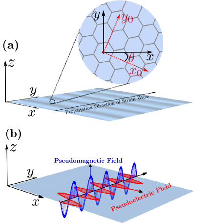
Figure 1: (Color online) (a) Schematic representation of a sound wave in graphene sample. The dark regions represent zones of higher density of carbon atoms in graphene sample. In the inset, the relation between the arbitrary coordinate system $xy$ and the crystalline coordinate system $x_{0}y_{0}$ is shown. (b) Unstrained graphene under a pseudoelectromagnetic wave: an equivalent description to the problem of strain wave. The pseudoelectric field lie in graphene plane, whereas the pseudomagnetic field is perpendicular to the graphene sample.

As discussed extensively in the literature, the electronic consequences of a nonuniform strain can be captured by means of an effective gauge field $\bi{A}$, which in the rotated frame $xy$ is given by [39],

$$A_{x} = \frac{\beta}{2a_{0}}\Bigl{(}(u_{xx}-u_{yy})\cos 3\theta-2u_{xy}\sin 3\theta\Bigr{)},$$

$$A_{y} = \frac{\beta}{2a_{0}}\Bigl{(}-2u_{xy}\cos 3\theta-(u_{xx}-u_{yy})\sin 3\theta\Bigr{)},$$ (2)

where $\beta\simeq 3$ is the electron Grüneisen parameter and $u_{ij}=(\partial_{i}u_{j}+\partial_{j}u_{i})/2$ is the symmetric strain tensor. From the expression for the effective gauge field, it is clear that $\bi{A}$ exhibits a periodicity of $2\pi/3$ in $\theta$, which reflects the discrete rotational invariance, i.e. the trigonal symmetry, of the underlying honeycomb lattice. As is well known, in graphene there are two inequivalent Dirac cones, located at special points of high-symmetry of the reciprocal lattice and usually denoted by $\bi{K}$ and $\bi{K}^{\prime}$. The fictitious field (2) has opposite signs at different valleys [4]. If for the valley $\bi{K}$ the effective gauge field is $\bi{A}$, then for the other valley $\bi{K}^{\prime}$ is given by $-\bi{A}$. This reflects the fact that elastic deformations do not violate the time-reversal symmetry [40]. Here, for simplicity we will deal with the $\bi{K}$ valley, since the other is analogous and obtainable by simply changing the sign of $\bi{A}$.

For the case of the deformation field (1), from (2), the following effective gauge field results:

$$\bi{A}=\frac{\beta u_{0}G}{2a_{0}}\sin(Gy-\omega t)(\cos 3\theta,-\sin 3\theta).$$ (3)

Hence the strain wave (1) gives rise to a pseudoelectromagnetic wave propagating along the $y$-axis at the velocity $v_{s}$. Here the associated pseudomagnetic field given by $\partial_{x}A_{y}-\partial_{y}A_{x}$ oscillates perpendicularly to the graphene sample (see figure 1 (b)). On the other hand, the associated pseudoelectric field given by $-\partial_{t}\bi{A}$ oscillates in the sample plane but, in general, it is not perpendicular to the propagation direction of the strain wave. Let us illustrate this peculiar behavior. For example, for $\theta=\pm\pi/2+2n\pi/3$, i.e. when the strain wave moves along the zigzag direction, the pseudoelectric field oscillates along the propagation direction of the pseudoelectromagnetic wave. Thus, for $\theta=\pm\pi/2+2n\pi/3$, the pseudoelectromagnetic wave (3) behaves more like a sort of longitudinal mechanical wave. Also, notice that for this case the pseudomagnetic field is zero. In contrast, for $\theta=n\pi/3$, i.e. when the strain wave moves along the armchair direction, the pseudoelectric fields oscillates transversally to the propagation direction of the pseudoelectromagnetic wave, as the expected behavior of a real electromagnetic wave.

Then including the strain-induced gauge field via minimal coupling, the effective Dirac equation reads

$$v_{F}\boldsymbol{\sigma}\cdot(-i\hbar\nabla-\bi{A})\boldsymbol{\Psi}=i\hbar\partial_{t}\boldsymbol{\Psi},$$ (4)

where $v_{F}=8\times 10^{5}\mbox{m/s}$ is the Fermi velocity and $\boldsymbol{\sigma}=(\sigma_{x},\sigma_{y})$ are Pauli matrices acting on sublattice space. This equation describes low-energy excitations of the electronic system in graphene under the strain wave.

3 Volkov-like states

From (3) one can clearly distinguish the periodicity of the effective gauge field $\bi{A}$ along the time direction. Therefore, one could think the standard use of the Floquet theory to analyze time-periodic Hamiltonians [41]. At the same time, $\bi{A}$ presents space periodicity along the $y$-direction, so that, Bloch (Floquet) theory could also be used. However, since $\bi{A}$ ultimately depends upon the plane phase $\phi=Gy-\omega t$ of the wave, to solve (4), we propose a spinor wavefunction $\boldsymbol{\Psi}$ of the form [42]

$$\boldsymbol{\Psi}(x,y,t)=\exp[i(k_{x}x+k_{y}y-Et/\hbar)]\boldsymbol{\Phi}(\phi),$$ (5)

and then, a Floquet analysis could be translated to the effective equation of the spinor, as carried out in $\boldsymbol{\Phi}(\phi)$ [43]. In relativistic mechanics, this procedure is equivalent to a jump into the light-cone frame of reference. In principle, $E,k_{x},k_{y}$ are just parameters of the ansatz. However, to recover the solution for an electron in undeformed graphene, obtained as $A_{0}\rightarrow 0$, it is needed that $E=\pm\hbar v_{F}(k_{x}^{2}+k_{y}^{2})^{-1/2}$, as is done in similar relativistic problems [43, 44, 45].

Our ansatz (5) was firstly used by Volkov to find exact solutions of the Dirac equation for relativistic fermions under a plane electromagnetic wave in vacuum [42]. It is worth mentioning that only in the case when the electromagnetic wave propagates in vacuum the solutions of the Dirac equation can be found in a simple closed form, these are the Volkov states. However, when one consider the interaction with a plane wave propagating in a medium with an index of refraction $n_{m}\neq 1$, the mathematical complexity of the Dirac equation is largely increased, and in fact, it is a problem with a long history (see for example [46, 47] and references therein).

Comparing our problem, given by (3) and (4), with the standard problem of real relativistic fermions under a plane electromagnetic wave in a medium with an index of refraction $n_{m}$, one can recognize the following. The Fermi velocity $v_{F}$ plays the role of the speed of light in vacuum $c$, whereas the strain wave velocity $v_{s}$ plays the role of the electromagnetic wave speed $c/n_{m}$ in a medium. From this analogy, one can think that our pseudoelectromagnetic wave propagates in a medium with effective index of refraction $n_{m}=v_{F}/v_{s}>1$, which is a different limiting than the one considered in the real electromagnetic case where $n_{m}<1$ [48]. Only in the hypothetical case that $v_{F}=v_{s}$, one can obtain the usual Volkov states [49].

Substituting (5) into (4) and taking into account $v_{F}\gg v_{s}$, we obtain the following differential system for the components of spinor $\boldsymbol{\Phi}(\phi)$,

$$\frac{\rmd\Phi_{B}}{\rmd\phi}=(\tilde{k}_{x}-i\tilde{k}_{y}-\tilde{A}_{0}e^{i3\theta}\sin\phi)\Phi_{B}-\tilde{E}\Phi_{A},$$

$$-\frac{\rmd\Phi_{A}}{\rmd\phi}=(\tilde{k}_{x}+i\tilde{k}_{y}-\tilde{A}_{0}e^{-i3\theta}\sin\phi)\Phi_{A}-\tilde{E}\Phi_{B},$$ (6)

where we define the non-dimensional parameters: $\tilde{k}_{x,y}=k_{x,y}/G$, $\tilde{A}_{0}=\beta u_{0}/(2a_{0})$ and $\tilde{E}=E/(\hbar v_{F}G)$. This system can be reduced to a second-order differential equation for each component of spinor $\boldsymbol{\Phi}(\phi)$, denoted by ${\Gamma}_{A}$ and ${\Gamma}_{B}$. However, before it is appropriate to carry out a new ansatz:

$$\boldsymbol{\Phi}(\phi)=\exp[-i\tilde{k}_{y}\phi+i\tilde{A}_{0}\sin 3\theta\cos\phi]\boldsymbol{\Gamma}(\phi).$$ (7)

As a result, from (3) and (7) we obtain that the both components ${\Gamma}_{A}$ and ${\Gamma}_{B}$ satisfy the Mathieu equation (see Appendix):

$$\frac{d^{2}\Gamma_{A,B}}{d\zeta^{2}}+(a-2q\cos\zeta)\Gamma_{A,B}=0,$$ (8)

where we introduce the variable

$$\zeta=(\phi+\phi_{0})/2,\ \ \ \mbox{with}\ \tan\phi_{0}=2\tilde{k}_{x},$$ (9)

and the new parameters

$$a=4\tilde{k}^{2}_{y},\ \ \mbox{and}\ \ q=2\tilde{A}_{0}(1+4\tilde{k}^{2}_{x})^{1/2}\cos 3\theta.$$ (10)

Therefore, the general solutions to the components ${\Gamma}_{A}$ and ${\Gamma}_{B}$ are linear combinations of the Mathieu cosine $C(a,q,\zeta)$ and Mathieu sine $S(a,q,\zeta)$ functions. Nevertheless, taking into account that when the pseudoelectromagnetic field is switched out ($\tilde{A}_{0}=0$) the wavefunction $\boldsymbol{\Psi}$ must reduce to a free-particle wavefunction, we get

$$\boldsymbol{\Gamma}(\zeta)=N(C(a,q,\zeta)+iS(a,q,\zeta))\left(\begin{array}[]{c}1\\ se^{i\alpha}\end{array}\right),$$ (11)

where $\alpha=\tan(\tilde{k}_{y}/\tilde{k}_{x})$, $N$ is a normalization constant and $s=\pm 1$ denotes the conduction and valence bands, respectively. To make sure that (11) reproduces the case of undeformed graphene, it is enough to consider the properties of the Mathieu functions for $q=0$: $C(a,0,\zeta)=\cos(\sqrt{a}\zeta)$ and $S(a,0,\zeta)=\sin(\sqrt{a}\zeta)$.

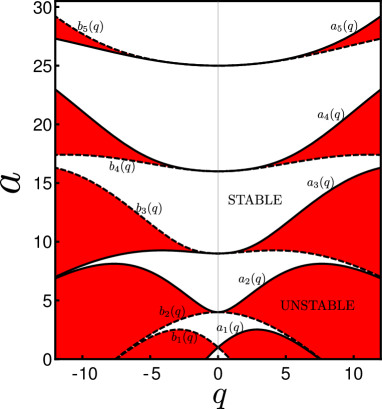
Figure 2: (Color online) Stability chart as a function of the non-dimensional parameters $a$ and $q$ for Mathieu solutions. The regions of stability (white domains) and instability (red domains) are divided by the characteristic curves $a_{n}(q)$ (solid lines) and $b_{n}(q)$ (dashed lines). The chart is symmetrical respect to the $a$-axis.

4 Discussion

As it is well documented [50], the stability of Mathieu functions depends on the parameters $a$ and $q$. In figure 2, the red regions in the ($a,q$)-plane are those for which the solutions are unstable (exponential functions) and therefore, are not acceptable from a quantum view point. On the other hand, the white regions are those for which the solutions are acceptable wavefunctions. The boundaries between these regions are determined by the eigenvalues, $a_{n}(q)$ and $b_{n}(q)$, corresponding to the $2\pi$-periodic Mathieu functions of integer order, $ce_{n}(q,\zeta)$ and $ce_{n}(q,\zeta)$, respectively [50].

As a consequence from the properties of Mathieu solutions mentioned above, a “band structure” naturally emerges in our problem. If one take into account (10), the stability chart in the ($a,q$)-plane is translated into a chart of the allowed bands in the ($\tilde{k}_{x},\tilde{k}_{y}$)-plane, as shown in figure 3 (a). When the strain wave propagates along the zigzag, $\cos 3\theta=0$, then $q=0$ and therefore the quasi-wave vector $\tilde{\bi{k}}=(\tilde{k}_{x},\tilde{k}_{y})$ can take any value. However, from the dependence $q\sim\cos 3\theta$, one can conclude that for a strain wave propagating along the armchair direction ($\cos 3\theta=\pm 1$), the band gaps in the ($\tilde{k}_{x},\tilde{k}_{y}$)-plane are expanded. Just for the sake of illustration, hereafter we consider $\theta=n\pi/3$.

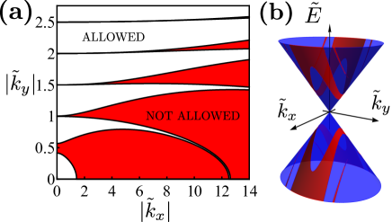
Figure 3: (Color online) Collimation effect of electron conduction by strain-waves. (a) Chart of the allowed bands (white regions) for the quasi momentum $\tilde{\bi{k}}$ (in units of $G$), with $\tilde{A}_{0}=0.15$ and the strain wave propagating along the armchair direction. The diagram is symmetrical respect to both axes. (b) Dirac cone. Red (blue) strips correspond to the forbidden (allowed) values of the quasi-energy $\tilde{E}(\tilde{k}_{x},\tilde{k}_{y})$ (in units of $\hbar v_{F}G$), because of the strain wave.

In figure 3 (a), we display the allowed values of the quasi-wave vector $\tilde{\bi{k}}=(\tilde{k}_{x},\tilde{k}_{y})$ for a strain wave of amplitude $u_{0}=0.1a_{0}$ and moves along the armchair direction. The most important result to notice in figure 3 (a) is that the quasi-particles propagate preferably in the $y$ direction, i.e., in the propagation direction of the strain wave leading to a collimation effect of the electrons. For example, notice that if $\tilde{k}_{y}=0$, the allowed values of $\tilde{k}_{x}$ are practically limited to the interval ($-q_{c}/4A_{0},q_{c}/4A_{0}$), where $b_{1}(q_{c}\approx 0.91)=0$. In other words, only low energy quasi-particles propagate perpendicularly to the propagation direction of the strain wave. On the contrary, for $\tilde{k}_{x}=0$, $|\tilde{k}_{y}|$ can take all values except basically those of the form $m/2$, where $m$ is a positive integer. This last result is an analogous condition as Bragg’s diffraction.

To end, let us point out that the forbidden values of the quasi-wave vector $\tilde{\bi{k}}$ divide the Dirac cone, given by $\tilde{E}=\pm(\tilde{k}_{x}+\tilde{k}_{y})^{1/2}$, into strips of allowed and forbidden values of the quasi-energy $\tilde{E}$, as illustrated in figure 3 (b). Similar results for the band structure have been discussed in earlies works for the case of a spin-less particle (which obeys the Klein-Gordon equation) in a medium (of $n_{m}>1$) irradiated with an electromagnetic plane wave [43, 44]. On the other hand, our results differ from those reported for graphene under an electromagnetic plane wave moves with the velocity of light in vacuum $c\approx 300v_{F}$ [48]. The physical reason is simple. In our problem, the pseudoelectromagnetic wave moves with the velocity of sound $v_{s}\approx v_{F}/40$.

Vaezi et al [36] reported the possibility of observing a nonvanishing charge current in graphene by applying a time-dependent strain. To archive this edge charge current, it was assumed a mass term to provide the presence of a gap in the spectrum, which is an essential ingredient to get a quantized response. From figure 3 (b) one can be distinguished that graphene remains gapless. Therefore, it does not seem possible to archive such edge charge currents in graphene under the considered approximations. To achieve a gap and thus topological modes as happens in the electromagnetic case [48], this will require a much higher amplitude of the strain than the one considered here since intervalley mixing is needed.

This is a consequence that in fact, there is a crucial difference between magnetic and pseudomagnetic fields. As commented above, the coupling constant for pseudomagnetic fields has opposite signs for electrons at different valleys, whereas for a magnetic field is the same. Since the coupling constant is valley anti-symmetric, the currents at the $\bi{K}$ and $\bi{K}’$ valleys flow in the opposite directions and they cancel out [37]. As a result, in general a pseudoelectric field does not cause a net electric current and thus adiabatic pumping is not possible as happens in the real electromagnetic fields [48]. Notice that in our case, the pseudomagnetic field can be considered as adiabatic since $\omega\ll Gv_{F}$.

5 Conclusion

In conclusion, we studied the effects of a strain wave on electron motion in graphene. The coupling between the quasi-particles and the strain wave are captured by means of an effective pseudoelectromagnetic wave. As solutions to the resulting effective Dirac equation, we found Volkov-type states, which propagates preferably in the propagation direction of deformation. Also, we reported a band structure of allowed and not allowed values for the quasi-momentum and for the quasi-energy. The form of the emergent band structure depends on the propagation direction of the strain wave respect to the crystalline directions of graphene lattice. This fact produces a collimation effect of charge carriers by strain waves, which should be an alternative mechanism to archive electron beam collimation, beyond magnetic focusing [51], an external periodic potential [52] or nanostructured heterodimensional graphene junctions [53].

Appendix

In this section, we present the details of the calculations to derive (8) from (3). Note that, the differential system (3) can be rewritten as

$$\frac{d\Phi_{B}}{d\phi}=(\tilde{k}_{x}-\tilde{A}_{0}\cos 3\theta\sin\phi-i\tilde{k}_{y}-i\tilde{A}_{0}\sin 3\theta\sin\phi)\Phi_{B}$$

$$\qquad-\tilde{E}\Phi_{A},$$

$$-\frac{d\Phi_{A}}{d\phi}=(\tilde{k}_{x}-\tilde{A}_{0}\cos 3\theta\sin\phi+i\tilde{k}_{y}+i\tilde{A}_{0}\sin 3\theta\sin\phi)\Phi_{A}$$

$$\qquad-\tilde{E}\Phi_{B}.$$

To simplify this system, one can propose that

$$\boldsymbol{\Phi}(\phi)=\exp[\int^{\phi}(-i\tilde{k}_{y}-iA_{0}\sin 3\theta\sin\phi^{*})d\phi^{*}]\boldsymbol{\Gamma}(\phi),$$

$$\qquad=\exp[-i\tilde{k}_{y}\phi+iA_{0}\sin 3\theta\cos\phi]\boldsymbol{\Gamma}(\phi),$$

and then one get the following differential system

$$\frac{d\Gamma_{B}}{d\phi}=(\tilde{k}_{x}-\tilde{A}_{0}\cos 3\theta\sin\phi)\Gamma_{B}-\tilde{E}\Gamma_{A},$$

$$-\frac{d\Gamma_{A}}{d\phi}=(\tilde{k}_{x}-\tilde{A}_{0}\cos 3\theta\sin\phi)\Gamma_{A}-\tilde{E}\Gamma_{B},$$

for the components of the spinor $\boldsymbol{\Gamma}(\phi)$. Now, taking second derivate one can reduce this last system to a Hill differential equation for both components $\Gamma_{A}$ and $\Gamma_{B}$:

$$\frac{d^{2}\Gamma_{A,B}}{d\phi^{2}}+[\tilde{E}^{2}-\tilde{A}_{0}\cos 3\theta\cos\phi-(\tilde{k}_{x}-\tilde{A}_{0}\cos 3\theta\sin\phi)^{2}]\Gamma_{A,B}=0.$$

However, since in the our problem $\tilde{A}_{0}=\beta u_{0}/(2a_{0})\ll 1$, the second-order terms in $\tilde{A}_{0}$ can be neglected, and taking into account that $\tilde{k}_{y}^{2}=\tilde{E}^{2}-\tilde{k}_{x}^{2}$, then one find that

$$\frac{d^{2}\Gamma_{A,B}}{d\phi^{2}}+[\tilde{k}_{y}^{2}-\tilde{A}_{0}\sqrt{1+4\tilde{k}^{2}_{x}}\cos 3\theta\cos(\phi+\phi_{0})]\Gamma_{A,B}=0.$$

where $\tan\phi_{0}=2\tilde{k}_{x}$. Finally, if one carry out the variable change $\zeta=(\phi+\phi_{0})/2$ and define the parameters $a=4\tilde{k}^{2}_{y}$ and $q=2\tilde{A}_{0}(1+4\tilde{k}^{2}_{x})^{1/2}\cos 3\theta$, one obtain (8), which is the Mathieu equation.

References

References

- [1] K. S. Novoselov et al. Electric field effect in atomically thin carbon films. Science, 306(5696):666–669, 2004.
- [2] A. K. Geim. Graphene: Status and prospects. Science, 324(5934):1530–1534, 2009.
- [3] K. S. Novoselov. Nobel lecture: Graphene: Materials in the flatland. Rev. Mod. Phys., 83:837–849, Aug 2011.
- [4] M. I. Katsnelson. Graphene: Carbon in Two Dimensions. Cambridge University Press, Cambridge, UK, 2012.
- [5] Andres Castellanos-Gomez, Vibhor Singh, Herre S. J. van der Zant, and Gary A. Steele. Mechanics of freely-suspended ultrathin layered materials. Annalen der Physik, 527(1-2):27–44, 2015.
- [6] Changgu Lee, Xiaoding Wei, Jeffrey W. Kysar, and James Hone. Measurement of the elastic properties and intrinsic strength of monolayer graphene. Science, 321(5887):385–388, 2008.
- [7] Zhen Hua Ni, Ting Yu, Yun Hao Lu, Ying Ying Wang, Yuan Ping Feng, and Ze Xiang Shen. Uniaxial strain on graphene: Raman spectroscopy study and band-gap opening. ACS Nano, 2(11):2301–2305, 2008.
- [8] Vitor M. Pereira, A. H. Castro Neto, and N. M. R. Peres. Tight-binding approach to uniaxial strain in graphene. Phys. Rev. B, 80:045401, Jul 2009.
- [9] Mark A. Bissett, Satoru Konabe, Susumu Okada, Masaharu Tsuji, and Hiroki Ago. Enhanced chemical reactivity of graphene induced by mechanical strain. ACS Nano, 7(11):10335–10343, 2013.
- [10] J. Atalaya, J. M. Kinaret, and A. Isacsson. Nanomechanical mass measurement using nonlinear response of a graphene membrane. EPL (Europhysics Letters), 91(4):48001, 2010.
- [11] A M Eriksson, D Midtvedt, A Croy, and A Isacsson. Frequency tuning, nonlinearities and mode coupling in circular mechanical graphene resonators. Nanotechnology, 24(39):395702, 2013.
- [12] Guang-Xin Ni, Hong-Zhi Yang, Wei Ji, Seung-Jae Baeck, Chee-Tat Toh, Jong-Hyun Ahn, Vitor M. Pereira, and Barbaros Özyilmaz. Tuning optical conductivity of large-scale cvd graphene by strain engineering. Advanced Materials, 26(7):1081–1086, 2014.
- [13] M. Oliva-Leyva and Gerardo G. Naumis. Tunable dichroism and optical absorption of graphene by strain engineering. 2D Materials, 2(2):025001, 2015.
- [14] Gerardo G. Naumis and Pedro Roman-Taboada. Mapping of strained graphene into one-dimensional hamiltonians: Quasicrystals and modulated crystals. Phys. Rev. B, 89:241404, Jun 2014.
- [15] Pedro Roman-Taboada and Gerardo G. Naumis. Spectral butterfly, mixed dirac-schrödinger fermion behavior, and topological states in armchair uniaxial strained graphene. Phys. Rev. B, 90:195435, Nov 2014.
- [16] G. Montambaux, F. Piéchon, J.-N. Fuchs, and M. O. Goerbig. Merging of dirac points in a two-dimensional crystal. Phys. Rev. B, 80:153412, Oct 2009.
- [17] R. de Gail, J.-N. Fuchs, M.O. Goerbig, F. Piéchon, and G. Montambaux. Manipulation of dirac points in graphene-like crystals. Physica B: Condensed Matter, 407(11):1948 – 1952, 2012.
- [18] G.E. Volovik and M.A. Zubkov. Emergent horava gravity in graphene. Annals of Physics, 340(1):352 – 368, 2014.
- [19] M.A. Zubkov. Emergent gravity and chiral anomaly in dirac semimetals in the presence of dislocations. Annals of Physics, 360:655 – 678, 2015.
- [20] D. A. Abanin and D. A. Pesin. Interaction-induced topological insulator states in strained graphene. Phys. Rev. Lett., 109:066802, Aug 2012.
- [21] Bitan Roy and Igor F. Herbut. Topological insulators in strained graphene at weak interaction. Phys. Rev. B, 88:045425, Jul 2013.
- [22] B. Amorim, A. Cortijo, F. de Juan, A. G. Grushin, F. Guinea, A. Gutiérrez-Rubio, H. Ochoa, V. Parente, R. Roldán, P. San-José, J. Schiefele, M. Sturla, and M. A. H. Vozmediano. Novel effects of strains in graphene and other two dimensional materials. arXiv:1503.00747, 2015.
- [23] N. Levy, S. A. Burke, K. L. Meaker, M. Panlasigui, A. Zettl, F. Guinea, A. H. Castro Neto, and M. F. Crommie. Strain-induced pseudo–magnetic fields greater than 300 tesla in graphene nanobubbles. Science, 329(5991):544–547, 2010.
- [24] Jiong Lu, A.H. Castro Neto, and Kian Ping Loh. Transforming moiré blisters into geometric graphene nano-bubbles. Nat Commun, 3:823, May 2012.
- [25] Hidekatsu Suzuura and Tsuneya Ando. Phonons and electron-phonon scattering in carbon nanotubes. Phys. Rev. B, 65:235412, May 2002.
- [26] F. Guinea, M. I. Katsnelson, and A. K. Geim. Energy gaps and a zero-field quantum hall effect in graphene by strain engineering. Nat Phys, 6(1):30–33, 2010.
- [27] Maria A. H. Vozmediano, M. I. Katsnelson, and F. Guinea. Gauge fields in graphene. Physics Reports, 496(4–5):109 – 148, 2010.
- [28] James V. Sloan, Alejandro A. Pacheco Sanjuan, Zhengfei Wang, Cedric Horvath, and Salvador Barraza-Lopez. Strain gauge fields for rippled graphene membranes under central mechanical load: An approach beyond first-order continuum elasticity. Phys. Rev. B, 87:155436, Apr 2013.
- [29] Diana A. Gradinar, Marcin Mucha-Kruczyński, Henning Schomerus, and Vladimir I. Fal’ko. Transport signatures of pseudomagnetic landau levels in strained graphene ribbons. Phys. Rev. Lett., 110:266801, Jun 2013.
- [30] Zenan Qi, Alexander L. Kitt, Harold S. Park, Vitor M. Pereira, David K. Campbell, and A. H. Castro Neto. Pseudomagnetic fields in graphene nanobubbles of constrained geometry: A molecular dynamics study. Phys. Rev. B, 90:125419, Sep 2014.
- [31] R. Carrillo-Bastos, D. Faria, A. Latgé, F. Mireles, and N. Sandler. Gaussian deformations in graphene ribbons: Flowers and confinement. Phys. Rev. B, 90:041411, Jul 2014.
- [32] Gareth W Jones and Vitor M Pereira. Designing electronic properties of two-dimensional crystals through optimization of deformations. New Journal of Physics, 16(9):093044, 2014.
- [33] M. Oliva-Leyva and Gerardo G. Naumis. Generalizing the fermi velocity of strained graphene from uniform to nonuniform strain. Physics Letters A, 379(40–41):2645 – 2651, 2015.
- [34] Felix von Oppen, Francisco Guinea, and Eros Mariani. Synthetic electric fields and phonon damping in carbon nanotubes and graphene. Phys. Rev. B, 80:075420, Aug 2009.
- [35] N E Firsova and Yu A Firsov. A new loss mechanism in graphene nanoresonators due to the synthetic electric fields caused by inherent out-of-plane membrane corrugations. Journal of Physics D: Applied Physics, 45(43):435102, 2012.
- [36] Abolhassan Vaezi, Nima Abedpour, Reza Asgari, Alberto Cortijo, and María A. H. Vozmediano. Topological electric current from time-dependent elastic deformations in graphene. Phys. Rev. B, 88:125406, Sep 2013.
- [37] Ken-ichi Sasaki, Hideki Gotoh, and Yasuhiro Tokura. Valley-antisymmetric potential in graphene under dynamical deformation. Phys. Rev. B, 90:205402, Nov 2014.
- [38] Vadym Adamyan and Vladimir Zavalniuk. Phonons in graphene with point defects. Journal of Physics: Condensed Matter, 23(1):015402, 2011.
- [39] Feng Zhai, Xiaofang Zhao, Kai Chang, and H. Q. Xu. Magnetic barrier on strained graphene: A possible valley filter. Phys. Rev. B, 82:115442, Sep 2010.
- [40] A. F. Morpurgo and F. Guinea. Intervalley scattering, long-range disorder, and effective time-reversal symmetry breaking in graphene. Phys. Rev. Lett., 97:196804, Nov 2006.
- [41] Milena Grifoni and Peter Hänggi. Driven quantum tunneling. Physics Reports, 304(5–6):229 – 354, 1998.
- [42] D.M. Wolkow. Über eine klasse von lösungen der diracschen gleichung. Zeitschrift für Physik, 94(3-4):250–260, 1935.
- [43] C. Cronström and M. Noga. Photon induced relativistic band structure in dielectrics. Physics Letters A, 60(2):137 – 139, 1977.
- [44] W. Becker. Relativistic charged particles in the field of an electromagnetic plane wave in a medium. Physica A: Statistical Mechanics and its Applications, 87(3):601 – 613, 1977.
- [45] V. B. Berestetskii, E. M. Lifshitz, and L. P. Pitaevskii. Quantum Electrodynamics, volume 4. Mir, Moscow, 2nd edition, 1982.
- [46] Sándor Varró. New exact solutions of the dirac equation of a charged particle interacting with an electromagnetic plane wave in a medium. Laser Physics Letters, 10(9):095301, 2013.
- [47] Sándor Varró. A new class of exact solutions of the klein–gordon equation of a charged particle interacting with an electromagnetic plane wave in a medium. Laser Physics Letters, 11(1):016001, 2014.
- [48] F. J. López-Rodríguez and G. G. Naumis. Analytic solution for electrons and holes in graphene under electromagnetic waves: Gap appearance and nonlinear effects. Phys. Rev. B, 78:201406, Nov 2008.
- [49] J. Bergou and S. Varró. Nonlinear scattering processes in the presence of a quantised radiation field. ii. relativistic treatment. Journal of Physics A: Mathematical and General, 14(9):2281, 1981.
- [50] N. McLachlan. Theory and Application of Mathieu Functions. Clarendon, New York, 1st edition, 1951.
- [51] H. van Houten, B. J. van Wees, J. E. Mooij, C. W. J. Beenakker, J. G. Williamson, and C. T. Foxon. Coherent electron focussing in a two-dimensional electron gas. EPL (Europhysics Letters), 5(8):721, 1988.
- [52] Cheol-Hwan Park, Young-Woo Son, Li Yang, Marvin L. Cohen, and Steven G. Louie. Electron beam supercollimation in graphene superlattices. Nano Letters, 8(9):2920–2924, 2008.
- [53] Zhengfei Wang and Feng Liu. Manipulation of electron beam propagation by hetero-dimensional graphene junctions. ACS Nano, 4(4):2459–2465, 2010.