Analytic Solutions to Large Deformation Problems Governed by Generalized Neo-Hookean Model

Abstract

This paper addresses some fundamental issues in nonconvex analysis. By using pure complementary energy principle proposed by the author, a class of fully nonlinear partial differential equations in nonlinear elasticity is able to converted a unified algebraic equation, a complete set of analytical solutions are obtained for 3-D finite deformation problems governed by generalized neo-Hookean model. Both global and local extremal solutions to the nonconvex variational problem are identified by a triality theory. Connection between challenges in nonlinear analysis and NP-hard problems in computational science is revealed. Results show that Legendre-Hadamard condition can only guarantee ellipticity for generalized convex problems. For nonconvex systems, the ellipticity depends not only on the stored energy, but also on the external force field. Uniqueness is proved based on a generalized quasiconvexity and a generalized ellipticity condition. Application is illustrated for nonconvex logarithm stored energy.

AMS Classification: 35Q74, 49S05, 74B20
Keywords: Nonlinear PDEs, Nonconvex analysis, Ellipticity, Nonlinear elasticity, Large deformation.

1 Nonconvex Variational Problem and Challenges

Minimum total potential energy principle in nonlinear elasticity has always presented fundamental challenging problems not only in continuum mechanics, but also in nonlinear analysis and computational sciences. This paper intends to solve, under certain conditions, the following minimum potential variational problem ($({\cal P})$ for short):

$$({\cal P}):\;\;\min\left\{\Pi(\mbox{\boldmath$\chi$})=\int_{{\cal B}}{W}(\nabla\mbox{\boldmath$\chi$}){\rm d}{\cal B}-\int_{S_{t}}\mbox{\boldmath$\chi$}\cdot{\bf t}{\rm d}S|\;\;\mbox{\boldmath$\chi$}\in{\cal{X}}_{c}\right\},$$ (1)

where the unknown deformation $\mbox{\boldmath$\chi$}({\bf x})=\{\chi_{i}(x_{j})\}\in{\cal{X}}_{a}$ is a vector-valued mapping ${\cal B}\subset\mathbb{R}^{3}\rightarrow\omega\subset\mathbb{R}^{3}$ from a given material particle ${\bf x}=\{x_{i}\}\in{\cal B}$ in the undeformed body to a position vector in the deformed configuration $\omega$. The body is fixed on the boundary $S_{x}\subset\partial{\cal B}$, while on the remaining boundary $S_{t}=S_{x}\cap\partial{\cal B}$, the body is subjected to a given surface traction ${\bf t}({\bf x})$. In this paper, we let ${\cal{X}}_{a}$ as a geometrically admissible space defined by

$${\cal{X}}_{a}=\{\mbox{\boldmath$\chi$}\in{\cal W}^{1,1}({\cal B};\mathbb{R}^{3})|\;\;\mbox{\boldmath$\chi$}({\bf x})=0\;\;\forall{\bf x}\in S_{x}\}$$ (2)

where ${\cal W}^{1,1}$ is the standard notation for Sobolev space, i.e. a function space in which both $\chi$ and its weak derivative $\nabla\mbox{\boldmath$\chi$}$ have a finite $L^{1}({\cal B})$ norm. For homogeneous hyperelastic body, the strain energy ${W}({\bf F})$ is assumed to be $C^{1}$ on its domain ${\cal{F}}_{c}\subset\mathbb{R}^{3\times 3}$, in which certain necessary constitutive constraints are included, such as

$$\det{\bf F}>0,\;\;{W}({\bf F})\geq 0\;\;\forall{\bf F}\in{\cal{F}}_{c},\;\;{W}({\bf F})\rightarrow\infty\mbox{ as }\|{\bf F}\|\rightarrow\infty.$$ (3)

Thus, the kinetically admissible space in $({\cal P})$ is simply defined by

$${\cal{X}}_{c}=\{\mbox{\boldmath$\chi$}\in{\cal{X}}_{a}|\;\nabla\mbox{\boldmath$\chi$}\in{\cal{F}}_{c}\}$$ (4)

which is essentially nonconvex due to nonlinear constraints such as $\det(\nabla\mbox{\boldmath$\chi$})>0$. Also, the stored energy ${W}({\bf F})$ is in general nonconvex in order to model real-world problems such as post-buckling and phase transitions, etc. Therefore, the nonconvex variational problem $({\cal P})$ has usually multiple local optimal solutions.

Let ${\cal{X}}_{b}\subset{\cal{X}}_{c}$ be a subspace with two additional conditions

$${\cal{X}}_{b}=\{\mbox{\boldmath$\chi$}\in{\cal{X}}_{c}|\;\;\mbox{\boldmath$\chi$}\in C^{2}({\cal B};\mathbb{R}^{3}),\;\;{W}({\bf F}(\mbox{\boldmath$\chi$}))\in C^{2}({\cal{F}}_{c};\mathbb{R})\}.$$ (5)

If $\partial{\cal B}$ is sufficiently regular, the criticality condition $\delta\Pi(\mbox{\boldmath$\chi$};\delta\mbox{\boldmath$\chi$})=0\;\;\forall\delta\mbox{\boldmath$\chi$}\in{\cal{X}}_{b}$ leads to a nonlinear boundary-value problem

$$(BVP):\;\;\;\left\{\begin{array}[]{l}-\nabla\cdot\mbox{\boldmath$\sigma$}(\nabla\mbox{\boldmath$\chi$})=0\;\;\mbox{ in }{\cal B},\\ {\bf N}\cdot\mbox{\boldmath$\sigma$}(\nabla\mbox{\boldmath$\chi$})={\bf t}\;\;\mbox{ on }S_{t},\;\;\mbox{\boldmath$\chi$}=0\;\;\mbox{ on }S_{x}\end{array}\right.$$ (6)

where, ${\bf N}\in\mathbb{R}^{3}$ is a unit vector normal to $\partial{\cal B}$, and $\mbox{\boldmath$\sigma$}({\bf F})$ is the first Piola-Kirchhoff stress (force per unit undeformed area), defined by

$$\mbox{\boldmath$\sigma$}=\nabla{W}({\bf F}),\;\;\mbox{ or }\;\sigma_{ij}=\frac{\partial{W}({\bf F})}{\partial F_{ij}},\;\;i,j=1,2,3.$$ (7)

Remark 1 (Nonconvexity, Multi-Solutions, and NP-Hard Problems)

 
The stored energy ${W}({\bf F})$ in nonlinear elasticity is generally nonconvex. It turns out that the fully nonlinear $(BVP)$ could have multiple solutions $\{\mbox{\boldmath$\chi$}_{k}({\bf x})\}\in{\cal{X}}_{c}\subset\mathbb{R}^{\infty}$ at each material point ${\bf x}\in{\cal B}_{s}\subset{\cal B}$. As long as the continuous domain ${\cal B}_{s}\neq\emptyset$, this solution set $\{\mbox{\boldmath$\chi$}_{k}({\bf x})\}(k=1,\dots,K)$ can form infinitely many ($K^{\infty}$) solutions to $(BVP)$ even ${\cal B}\subset\mathbb{R}$. It is impossible to use traditional convexity and ellipticity conditions to identify global minimizer among all these local solutions. Gao and Ogden discovered in [11] that for certain given external force field, both global and local extremum solutions are nonsmooth and can’t be obtained by Newton-type numerical methods. Therefore, Problem $({\cal P})$ is much more difficult than $(BVP)$. In computational mechanics, any direct numerical method for solving $({\cal P})$ will lead to a nonconvex minimization problem in $\mathbb{R}^{n}$, which could have $K^{n}$ local solutions. Due to the lack of global optimality condition, it is fundamentally difficult to solve nonconvex minimization problems by traditional methods within polynomial time. Therefore, in computational sciences most nonconvex minimization problems are considered to be NP-hard (Non-deterministic Polynomial-time hard) [12].

Direct methods for solving nonconvex variational problems in finite elasticity have been studies extensively during the last fifty years and many generalized convexities, such as poly-, quasi- and rank-one convexities, have been proposed. For a given function $W:{\cal{F}}_{c}\rightarrow\mathbb{R}$, the following statements are well-known (see [19]):

convex $$\Rightarrow\mbox{ poly-convex }\Rightarrow\mbox{ quasi-convex }\Rightarrow\mbox{ rank-one convex}$$.

Although the generalized convexities have been well-studied for general function ${W}({\bf F})$ on matrix space $\mathbb{R}^{m\times n}$, these mathematical concepts provide only necessary conditions for local minimal solutions, and can’t be applied to general (nonconvex) finite deformation problems. In reality, the stored energy ${W}({\bf F})$ must be nonconvex in order to model real-world phenomena. Strictly speaking, due to certain necessary constitutive constraints such as $\det{\bf F}>0$ and objectivity condition etc, even the domain ${\cal{F}}_{c}$ is not convex, therefore, it is not appropriate to discuss convexity of the stored energy ${W}({\bf F})$ in general nonlinear elasticity. How to identify global optimal solution has been a fundamental challenging problem in nonconvex analysis and computational science. $\blacksquare$

Remark 2 (Canonical Duality, Gap Function, and Global Extremality)

 
The objectivity is a necessary constraint for any hyper-elastic model. A real-valued function ${W}:{\cal{F}}_{c}\rightarrow\mathbb{R}$ is objective iff there exists a function $V({\bf C})$ such that $W({\bf F})=V({\bf F}^{T}{\bf F})\;\;\forall{\bf F}\in{\cal{F}}_{c}$ (see [2]). By the fact that the right Cauchy-Green tensor ${\bf C}$ is an objective measure on a convex domain ${\cal{E}}_{a}=\{{\bf C}\in\mathbb{R}^{3\times 3}|\;\;{\bf C}={\bf C}^{T},\;\;{\bf C}\succ 0\}$, it is possible and natural to discuss the convexity of $V({\bf C})$. A real-valued function $V:{\cal{E}}_{a}\rightarrow\mathbb{R}$ is called canonical if the duality relation $\mbox{\boldmath$\xi$}^{*}=\nabla V(\mbox{\boldmath$\xi$}):{\cal{E}}_{a}\rightarrow{\cal{E}}^{*}_{a}$ is one-to-one and onto [6]. The canonical duality is necessary for modeling natural phenomena, which lays a foundation for the canonical duality theory [6]. This theory was developed from Gao and Strang’s original work in 1989 [13] for general nonconvex/nonsmooth variational problems in finite deformation theory. The key idea of this theory is assuming the existence of a geometrically admissible (objective) measure $\mbox{\boldmath$\xi$}=\Lambda({\bf F})$ and a canonical function $V(\mbox{\boldmath$\xi$})$ such that the following canonical transformation holds

$$\mbox{\boldmath$\xi$}=\Lambda({\bf F}):{\cal{F}}_{a}\rightarrow{\cal{E}}_{a}\;\;\Rightarrow\;\;{W}({\bf F})=V(\Lambda({\bf F})).$$ (8)

Gao and Strang discovered that the directional derivative ${\Lambda}_{t}({\bf F})=\delta{\Lambda}({\bf F})$ is adjoined with the equilibrium operator, while its complementary operator ${\Lambda}_{c}({\bf F})=\Lambda({\bf F})-{\Lambda}_{t}({\bf F}){\bf F}$ leads to a so-called complementary gap function, which recovers duality gaps in traditional duality theories and provides a sufficient condition for identifying both global and local extremal solutions [6, 12].   $\blacksquare$

The canonical duality theory has been applied for solving a large class of nonconvex, nonsmooth, discrete problems in multidisciplinary fields of nonlinear analysis, nonconvex mechanics, global optimization, and computational sciences, etc. A comprehensive review is given recently in [12]. The main goal of this paper is to show author’s recent analytical solutions [8] for general anti-plane shear problems can be easily generalized for solving finite deformation problems governed by generalized neo-Hookean materials. Some insightful results are obtained on generalized convexity and ellipticity in nonlinear analysis.

2 Complete Solutions to Generalized Neo-Hookean Material

By the fact that the right Cauchy-Green strain ${\bf C}={\bf F}^{T}{\bf F}$ is an objective tensor, its three principal invariants

$$I_{1}({\bf C})=\mbox{tr\hskip 1.0pt}\mathbf{C},\quad I_{2}({\bf C})=\frac{1}{2}[(\mbox{tr\hskip 1.0pt}{\bf C})^{2}-\mbox{tr\hskip 1.0pt}({\bf C}^{2})],\quad I_{3}({\bf C})=\det\mathbf{C}$$ (9)

are also objective functions of ${\bf F}$. Clearly, for isochoric deformations we have $I_{3}({\bf C})=1$. The elastic body is said to be generalized neo-Hookean material if the stored energy depends only on $I_{1}$, i.e. there exists a function $V(I_{1})$ such that $W({\bf F})=V(I_{1}({\bf C}({\bf F})))$. Since $I_{1}=\mbox{tr\hskip 1.0pt}({\bf F}^{T}{\bf F})>0\;\;\forall{\bf F}\in{\cal{F}}_{c}$, the domain of $V(I_{1})$ is a convex (positive) cone

$${\cal{E}}_{a}=\{\xi\in L^{p}({\cal B})\;|\;\xi({\bf x})>0\;\;\forall{\bf x}\in{\cal B}\},$$ (10)

it is possible to discuss the convexity of $V(I_{1})$ on ${\cal{E}}_{a}$. Furthermore, we assume that $V(I_{1})$ is a $C^{2}({\cal{E}}_{a})$ canonical function. Then the canonical transformation (8) for the generalized neo-Hookean model is

$$\xi={\Lambda}({\bf F})=\mbox{tr\hskip 1.0pt}({\bf F}^{T}{\bf F}):{\cal{F}}_{c}\rightarrow{\cal{E}}_{a},\;\;{W}({\bf F})=V(\xi({\bf F})).$$ (11)

For a given external force ${\bf t}({\bf x})$ on ${S_{t}}$, we introduce a statically admissible space

$${{\cal{T}}}_{a}=\left\{{{\bf T}}\in{\cal W}^{1,1}({\cal B};\mathbb{R}^{3\times 3})\;|\;\;\nabla\cdot{\bf T}=0\;\;\mbox{ in }{\cal B},\;\;{\bf N}\cdot{\bf T}={\bf t}\;\;\;\mbox{ on }{S_{t}}\right\}.$$ (12)

Thus for any given ${\bf T}\in{\cal{T}}_{a}$, the primal problem $({\cal P})$ for the generalized neo-Hookean material can be written in following canonical form

$$({\cal P})_{{\bf T}}:\;\;\min\left\{\Pi_{\bf T}(\nabla\mbox{\boldmath$\chi$})=\int_{{\cal B}}G(\nabla\mbox{\boldmath$\chi$})\;{\rm d}{\cal B}\;\;|\;\;\forall\mbox{\boldmath$\chi$}\in{\cal{X}}_{c}\right\},$$ (13)

where ${\cal{X}}_{c}=\{\mbox{\boldmath$\chi$}\in{\cal{X}}_{a}|\;\Lambda(\nabla\mbox{\boldmath$\chi$})\in{\cal{E}}_{a}\}$ and the integrand $G:{\cal{F}}_{a}\rightarrow\mathbb{R}$ is defined by

$$G({\bf F})=V(\Lambda({\bf F}))-\mbox{tr\hskip 1.0pt}({\bf F}^{T}{\bf T}).$$ (14)

By the fact that $\det{\bf F}>0$ is not a variational constraint and the certain constitutive constraints, such as coercivity and objectivity, have been naturally relaxed by the canonical transformation, the domain of $G({\bf F})$ is simply ${\cal{F}}_{a}=\mathbb{R}^{3\times 3}$.

Let $\mbox{SO}(3)=\{{\bf R}\in\mathbb{R}^{3\times 3}|\;\;{\bf R}^{T}={\bf R}^{-1},\;\;\det{\bf R}=1\}$ and

$${\cal{R}}=\{{\bf R}({\bf x})\in L^{1}[{\cal B},\mathbb{R}^{3\times 3}]|\;\;{\bf R}({\bf x})\in\mbox{SO}(3)\;\;\forall{\bf x}\in{\cal B}\}.$$ (15)

Theorem 1

For any given ${\bf T}\in{\cal{T}}_{a}$, if $\bar{\mbox{\boldmath$\chi$}}\in{\cal{X}}_{c}$ is a stationary solution to $({\cal P})_{\bf T}$, then it is also a stationary solution to $({\cal P})$.

For any given rotation field ${\bf R}({\bf x})\in{\cal{R}}$ such that ${\bf R}^{T}{\bf T}\in{\cal{T}}_{a}$, then $\Pi_{{\bf T}}({\bf F})=\Pi_{{\bf T}}({\bf R}{\bf F})$.

For any uniform rotation ${\bf R}\in\mbox{SO}(3)$ such that ${\bf R}^{T}{\bf T}\in{\cal{T}}_{a}$, if $\bar{\mbox{\boldmath$\chi$}}$ is a stationary solution to $({\cal P})$, then ${\bf R}\bar{\mbox{\boldmath$\chi$}}$ is also a stationary solution to $({\cal P})$.

Proof. For any given ${\bf T}\in{\cal{T}}_{a}$, the stationary condition for the canonical variational problem $({\cal P})_{\bf T}$ leads to the following canonical boundary value problem

$$(BVP)_{{\bf T}}:\;\;\left\{\begin{array}[]{l}\nabla\cdot(2\zeta\nabla\mbox{\boldmath$\chi$})=\nabla\cdot{\bf T}=0\;\;\mbox{ in }{\cal B},\\ {\bf N}\cdot(2\zeta\nabla\mbox{\boldmath$\chi$})={\bf N}\cdot{\bf T}={\bf t}\;\mbox{ on }{S_{t}},\;\;\mbox{\boldmath$\chi$}=0\;\;\mbox{ on }S_{x}\end{array}\right.$$ (16)

which is identical to $(BVP)$ since

$$\mbox{\boldmath$\sigma$}=\nabla{W}({\bf F})=\frac{\partial V(\xi)}{\partial\xi}\frac{\partial\xi}{\partial{\bf F}}=2\zeta{\bf F},\;\;\zeta=\nabla V(\xi).$$

By the objectivity of $\xi=\Lambda({\bf F})=\Lambda({\bf R}{\bf F})\;\;\forall{\bf R}({\bf x})\in{\cal{R}}$ and the fact that

$$\int_{{\cal B}}\mbox{tr\hskip 1.0pt}[({\bf R}\nabla\mbox{\boldmath$\chi$})^{T}{\bf T}]{\rm d}{\cal B}=\int_{{\cal B}}\mbox{tr\hskip 1.0pt}[(\nabla\mbox{\boldmath$\chi$})^{T}({\bf R}^{T}{\bf T})]{\rm d}{\cal B}=\int_{S_{t}}\mbox{\boldmath$\chi$}\cdot{\bf t}{\rm d}S\;\;\forall{\bf R}^{T}{\bf T}\in{\cal{T}}_{a},$$

we have $\Pi_{{\bf T}}({\bf F})=\Pi_{\bf T}({\bf R}{\bf F})\;\;\forall{\bf R}({\bf x})\in{\cal{R}}$. Particularly, for any uniform ${\bf R}\in\mbox{SO}(3)$ such that ${\bf R}^{T}{\bf T}\in{\cal{T}}_{a}$, we have $\Pi(\mbox{\boldmath$\chi$})=\Pi_{{\bf T}}({\bf R}{\bf F}(\mbox{\boldmath$\chi$}))$. $\Box$

Theorem 1 is important for understanding the canonical duality theory.

By the canonical assumption on $V(\xi)$, the duality relation $\zeta=\nabla V(\xi):{\cal{E}}_{a}\rightarrow{\cal{E}}^{*}_{a}$ is invertible. The complementary energy can be defined uniquely by the Legendre transformation

$$V^{*}(\zeta)=\{\xi\zeta-V(\xi)|\;\zeta=\nabla V(\xi)\}.$$ (17)

Clearly, the function $V:{\cal{E}}_{a}\rightarrow\mathbb{R}$ is canonical if and only if the following canonical duality relations hold on ${\cal{E}}_{a}\times{\cal{E}}^{*}_{a}$

$$\zeta=\nabla V(\xi)\;\;\Leftrightarrow\;\;\xi=\nabla V^{*}(\zeta)\;\;\Leftrightarrow\;\;V(\xi)+V^{*}(\zeta)=\xi\zeta.$$ (18)

Using $V(\xi)=\xi\zeta-V^{*}(\zeta)$, the nonconvex function $G({\bf F})$ can be written as the standard Gao and Strang total complementary function $\Xi:{\cal{X}}_{a}\times{\cal{E}}^{*}_{a}\rightarrow\mathbb{R}$

$$\Xi(\mbox{\boldmath$\chi$},\zeta)=\int_{{\cal B}}\left[{\Lambda}(\nabla\mbox{\boldmath$\chi$})\zeta-V^{*}(\zeta)-\mbox{tr\hskip 1.0pt}((\nabla\mbox{\boldmath$\chi$})^{T}{\bf T})\right]{\rm d}{\cal B}.$$ (19)

Let ${\cal{S}}_{a}\subset{\cal{E}}^{*}_{a}$ be a canonical dual feasible space defined by

$${\cal{S}}_{a}=\{\zeta\in{\cal{E}}^{*}_{a}|\;\zeta^{-1}\tau^{2}\in L^{1}({\cal B})\}.$$ (20)

Then for a given $\zeta\in{\cal{S}}_{a}$, the canonical dual function can be obtained by the canonical dual transformation:

$$\Pi^{d}(\zeta)={\rm sta}\{\Xi(\mbox{\boldmath$\chi$},\zeta)|\;\;\mbox{\boldmath$\chi$}\in{\cal{X}}_{a}\}=\int_{{\cal B}}G^{d}(\zeta){\rm d}{\cal B},$$ (21)

where the notation ${\rm sta}\{\Xi(\mbox{\boldmath$\chi$},\zeta)|\;\mbox{\boldmath$\chi$}\in{\cal{X}}_{a}\}$ stands for finding (partial) stationary point $\mbox{\boldmath$\chi$}\in{\cal{X}}_{a}$ of $\Xi(\mbox{\boldmath$\chi$},\zeta)$ for a given $\zeta\in{\cal{S}}_{a}$, and

$$G^{d}(\zeta)=-V^{*}(\zeta)-\frac{1}{4}\zeta^{-1}\tau^{2},\;\;\;\;\tau^{2}=\mbox{tr\hskip 1.0pt}({\bf T}^{T}{\bf T}).$$ (22)

Thus, the pure complementary energy principle, first proposed in 1998 [4], leads to the following canonical dual variational problem

$$({\cal P}^{d}):\;\;\;\;{\rm sta}\left\{\Pi^{d}(\zeta)=\int_{{\cal B}}G^{d}(\zeta){\rm d}{\cal B}\;|\;\;\zeta\in{\cal{S}}_{a}\right\}.$$ (23)

Since the canonical dual variable $\zeta$ is a scalar-valued function, the criticality condition for this variational problem leads to a so-called canonical dual algebraic equation (see [6]):

$$4\zeta^{2}\nabla V^{*}(\zeta)=\tau^{2}({\bf x})\;\;\;\;\forall{\bf x}\in{\cal B}.$$ (24)

Note that $\nabla V^{*}(\zeta):{\cal{E}}^{*}_{a}\rightarrow{\cal{E}}_{a}$ is also one-to-one and onto, this equation has at least one solution for any given $\tau^{2}=\mbox{tr\hskip 1.0pt}({\bf T}^{T}{\bf T})\geq 0$ and $\zeta=0$ only if $\tau=0$. Therefore, although there is an inverse term $\zeta^{-1}$ in $G^{d}(\zeta)$, this canonical dual function is well-defined on ${\cal{S}}_{a}$. Due to the nonlinearity, the solution to (24) may not be unique [6, 8, 11]. By the pure complementary energy principle proposed by Gao in 1999 (see [6]), we have

Theorem 2 (Complementary-Dual Principle)

For any given ${\bf T}\in{\cal{T}}_{a}$, the following statements are equivalent:

1) $(\bar{\mbox{\boldmath$\chi$}},{\bar{\varsigma}})$ is a stationary point of $\Xi(\mbox{\boldmath$\chi$},\zeta)$;

2) $\bar{\mbox{\boldmath$\chi$}}$ is a stationary solution to $({\cal P})$;

3) ${\bar{\varsigma}}$ is a stationary solution to $({\cal P}^{d})$.

Moreover, we have

$$\Pi(\bar{\mbox{\boldmath$\chi$}})=\Xi(\bar{\mbox{\boldmath$\chi$}},{\bar{\varsigma}})=\Pi^{d}({\bar{\varsigma}})$$ (25)

Proof. For any given ${\bf T}\in{\cal{T}}_{a}$, the stationary condition of $\Xi(\mbox{\boldmath$\chi$},\zeta)$ leads to the canonical equilibrium equations

$$\Lambda({\bf F}(\bar{\mbox{\boldmath$\chi$}}))=\nabla V^{*}({\bar{\varsigma}}),$$ (26)

$$2{\bar{\varsigma}}{\bf F}(\bar{\mbox{\boldmath$\chi$}})={\bf T}\in{\cal{T}}_{a}$$ (27)

By the canonical duality, (26) is equivalent to ${\bar{\varsigma}}=\nabla V(\xi)$ with $\xi={\Lambda}(\nabla\bar{\mbox{\boldmath$\chi$}})$. Thus, $\bar{\mbox{\boldmath$\chi$}}$ must be a stationary solution to $({\cal P})_{{\bf T}}$ and also a stationary solution to $({\cal P})$ due to Theorem 1.

By solving (27) we have ${\bf F}(\bar{\mbox{\boldmath$\chi$}})=\frac{1}{2{\bar{\varsigma}}}{\bf T}$. Substituting this into (26) leads to the canonical dual equation (24). Thus, ${\bar{\varsigma}}$ is a stationary solution to $({\cal P}^{d})$.

The equivalence and the equation (25) can be proved by

$${\rm sta}\{\Pi_{{\bf T}}(\nabla\mbox{\boldmath$\chi$})|\;\mbox{\boldmath$\chi$}\in{\cal{X}}_{c}\}={\rm sta}\{\Xi(\mbox{\boldmath$\chi$},\zeta)|\;\;(\mbox{\boldmath$\chi$},\zeta)\in{\cal{X}}_{a}\times{\cal{E}}^{*}_{a}\}={\rm sta}\{\Pi^{d}(\zeta)|\;\;\zeta\in{\cal{S}}_{a}\}$$

and Theorem 1. $\Box$

Theorem 3 (Pure Complementary Energy Principle)

For any given nontrivial ${\bf t}\neq 0$ and $\mbox{\boldmath$\chi$}\in{\cal{X}}_{a}$ such that ${\bf T}\in{\cal{T}}_{a}\neq\emptyset$, (24) has at least one solution $\zeta_{k}\neq 0$, the deformation gradient defined by ${\bf F}_{k}=\nabla\mbox{\boldmath$\chi$}_{k}=\zeta_{k}^{-1}{\bf T}$ is a critical point of $\Pi(\mbox{\boldmath$\chi$})$ and $\Pi(\mbox{\boldmath$\chi$}_{k})=\Pi^{d}(\zeta_{k})$.

Moreover, if $\nabla\times(\zeta_{k}^{-1}{\bf T})=0$, then the deformation vector defined by

$$\mbox{\boldmath$\chi$}_{k}({\bf x})=\frac{1}{2}\int_{{\bf x}_{0}}^{\bf x}\zeta_{k}^{-1}{\bf T}\cdot\mbox{d}{\bf x}$$ (28)

along any path from ${\bf x}_{0}\in S_{x}$ to ${\bf x}\in{\cal B}$ is a solution to $(BVP)_{\bf T}$ in the sense that it satisfies both equilibrium equation and boundary conditions in (16).

Proof. By the canonical duality relations in (18) we know that $\xi_{k}=\nabla V^{*}(\zeta_{k})>0$. Thus, for a given nontrivial ${\bf t}({\bf x})$, there exists a nontrivial $\tau^{2}({\bf x})=\mbox{tr\hskip 1.0pt}({\bf T}^{T}{\bf T})$ in ${\cal B}$ such that the canonical dual algebraic equation (24) have at least one nontrivial solution $\zeta_{k}({\bf x})$ in ${\cal B}$.

Since the critical point $\zeta_{k}$ is a solution to (24), we have

$$\xi_{k}=\mbox{tr\hskip 1.0pt}({\bf F}^{T}_{k}{\bf F}_{k})=\frac{1}{4}\zeta_{k}^{-2}\mbox{tr\hskip 1.0pt}({\bf T}^{T}{\bf T})=\nabla V^{*}(\zeta_{k})\;\;\Rightarrow\;\;{\bf F}_{k}=\frac{1}{2}\zeta_{k}^{-1}{\bf T}$$ (29)

subjected to any given rotation field ${\bf R}({\bf x})\in{\cal{R}}$. By the fact that the canonical dual solution $\zeta_{k}$ defined by (24) is independent of the rotation field, the canonical duality leads to

$$G^{d}(\zeta_{z})=\Xi({\bf F}_{k},\zeta_{k})=V(\Lambda({\bf F}_{k}))-\mbox{tr\hskip 1.0pt}({\bf F}_{k}^{T}{\bf T})=G({\bf F}_{k}).$$

This shows $\Pi(\mbox{\boldmath$\chi$}_{k})=\Pi^{d}(\zeta_{k})$.

To prove $\mbox{\boldmath$\chi$}_{k}$ defined by (28) is a solution to $(BVP)_{\bf T}$, we simply substitute $\nabla\mbox{\boldmath$\chi$}_{k}={\bf F}_{k}=\frac{1}{2}\zeta_{k}^{-1}{\bf T}$ into $(BVP)_{\bf T}$ to have all necessary equilibrium conditions satisfied. Therefore, $\mbox{\boldmath$\chi$}_{k}$ defined by (28) is a solution to $(BVP)_{\bf T}$. $\Box$

This pure complementary energy principle shows that by the canonical dual transformation, the fully nonlinear partial differential equation in $(BVP)_{\bf T}$ can be converted to an algebraic equation (24), which can be solved to obtain a complete set of solutions (see [8, 9]).

Since ${\cal{S}}_{a}$ is nonconvex, in order to identify global and local optimal solutions, we need the following convex subsets

$${\cal{S}}_{a}^{+}=\{\zeta\in{\cal{S}}_{a}|\;\zeta>0\},\;\;\;{\cal{S}}_{a}^{-}=\{\zeta\in{\cal{S}}_{a}|\;\zeta<0\}.$$ (30)

Then by the canonical duality-triality theory developed in [6] we have the following theorem.

Theorem 4

Suppose that $V:{\cal{E}}_{a}\rightarrow\mathbb{R}$ is convex and for a given ${\bf T}\in{\cal{T}}_{a}$ such that $\{\zeta_{k}\}$ is a solution set to (24), ${\bf F}_{k}=\frac{1}{2}\zeta^{-1}_{k}{\bf T}$, and $\mbox{\boldmath$\chi$}_{k}$ is defined by (28), we have the following statements.

1. If $\zeta_{k}\in{\cal{S}}_{a}^{+}$, then $\nabla^{2}{W}({\bf F}_{k})\succ 0$ and $\mbox{\boldmath$\chi$}_{k}$ is a global minimal solution to $({\cal P})$.

2. If $\zeta_{k}\in{\cal{S}}_{a}^{-}$ and $\nabla^{2}{W}({\bf F}_{k})\succ 0$, then $\mbox{\boldmath$\chi$}_{k}$ is a local minimal solution to $({\cal P})$.

3. If $\zeta_{k}\in{\cal{S}}_{a}^{-}$ and $\nabla^{2}{W}({\bf F}_{k})\prec 0$, then $\mbox{\boldmath$\chi$}_{k}$ is a local maximal solution to $({\cal P})$.

If $\{\zeta_{k}\}\subset\bar{\cal{S}}^{+}_{a}$, then $\{\mbox{\boldmath$\chi$}_{k}\}$ is a convex set. The solution of $({\cal P})$ is unique if $\{\zeta_{k}\}\subset{\cal{S}}^{+}_{a}$.

Proof. By using chain rule for ${W}({\bf F})=V(\xi({\bf F}))$ we have $\nabla{W}({\bf F})=2{\bf F}[\nabla V(\xi)]=2\zeta{\bf F}$, and

$$\nabla^{2}{W}({\bf F})=2\zeta{\bf I}\otimes{\bf I}+4h(\xi){\bf F}\otimes{\bf F},$$ (31)

where $\mathbf{I}$ is an identity tensor in $\mathbb{R}^{3\times 3}$, $h(\xi)=\nabla^{2}V(\xi)\geq 0$ due to the convexity of $V$ on ${{\cal{E}}_{a}}$. Therefore, $\nabla^{2}{W}({\bf F}_{k})\succ 0$ if $\zeta_{k}\in{\cal{S}}^{+}_{a}$.

To prove $\mbox{\boldmath$\chi$}_{k}$ is a global minimizer of $({\cal P})$, we follow Gao and Strang’s work in 1989 [13]. By the convexity of $V(\xi)$ on its convex domain ${\cal{E}}_{a}$, we have

$$V(\xi)-V(\xi_{k})\geq(\xi-\xi_{k})\zeta_{k}\;\;\;\;\forall\xi,\;\xi_{k}\in{\cal{E}}_{a},\;\;\zeta_{k}=\nabla V(\xi_{k}).$$ (32)

For any given variation $\delta\mbox{\boldmath$\chi$}$, we let $\mbox{\boldmath$\chi$}=\mbox{\boldmath$\chi$}_{k}+\delta\mbox{\boldmath$\chi$}$. Then we have [13]

$$\Lambda(\nabla\mbox{\boldmath$\chi$})=\mbox{tr\hskip 1.0pt}[(\nabla\mbox{\boldmath$\chi$})^{T}(\nabla\mbox{\boldmath$\chi$})]=\Lambda(\nabla\mbox{\boldmath$\chi$}_{k})+{\Lambda}_{t}(\nabla\mbox{\boldmath$\chi$}_{k})(\nabla\delta\mbox{\boldmath$\chi$})-\Lambda_{c}(\nabla\delta\mbox{\boldmath$\chi$}),$$ (33)

where ${\Lambda}_{t}({\bf F})\delta{\bf F}=2\mbox{tr\hskip 1.0pt}[{\bf F}^{T}(\delta{\bf F})]$ and $\Lambda_{c}(\delta\mbox{\boldmath$\chi$})=-\Lambda(\delta\mbox{\boldmath$\chi$})$. Clearly, ${\Lambda}({\bf F})={\Lambda}_{t}({\bf F}){\bf F}+{\Lambda}_{c}({\bf F})$. Then combining the inequality (32) and (33), we have

$$\Pi(\mbox{\boldmath$\chi$})-\Pi(\mbox{\boldmath$\chi$}_{k}) \geq \int_{\cal B}2\zeta_{k}\mbox{tr\hskip 1.0pt}[(\nabla\mbox{\boldmath$\chi$}_{k})^{T}(\nabla\delta\mbox{\boldmath$\chi$})]{\rm d}{\cal B}-\int_{S_{t}}\delta\mbox{\boldmath$\chi$}\cdot{\bf t}{\rm d}S+\int_{\cal B}\zeta_{k}\mbox{tr\hskip 1.0pt}[(\nabla\mbox{\boldmath$\chi$})^{T}(\nabla\mbox{\boldmath$\chi$})]{\rm d}{\cal B}$$ (34)

$$= \int_{\cal B}[2\zeta_{k}(\nabla\mbox{\boldmath$\chi$}_{k})-{\bf T}]:(\nabla\delta\mbox{\boldmath$\chi$}){\rm d}{\cal B}+G_{ap}(\delta\mbox{\boldmath$\chi$},\zeta_{k})\;\;\forall\mbox{\boldmath$\chi$},\;\delta\mbox{\boldmath$\chi$}\in{\cal{X}}_{c}$$

for any given ${\bf T}\in{\cal{T}}_{a}$, where

$$G_{ap}(\mbox{\boldmath$\chi$},\zeta)=\int_{\cal B}-\Lambda_{c}(\nabla\mbox{\boldmath$\chi$})\zeta{\rm d}{\cal B}=\int_{\cal B}\zeta\mbox{tr\hskip 1.0pt}[(\nabla\mbox{\boldmath$\chi$})^{T}(\nabla\mbox{\boldmath$\chi$})]{\rm d}{\cal B}$$ (35)

is the complementary gap function introduced by Gao and Strang in [13]. If $\mbox{\boldmath$\chi$}_{k}$ is a critical point of $\Pi(\mbox{\boldmath$\chi$})$, then we have

$$\int_{\cal B}[2(\nabla\mbox{\boldmath$\chi$}_{k})\zeta_{k}-{\bf T}]:(\nabla\delta\mbox{\boldmath$\chi$}){\rm d}{\cal B}=0\;\;\forall\delta\mbox{\boldmath$\chi$}\in{\cal{X}}_{c},\;\;\forall{\bf T}\in{\cal{T}}_{a}$$

Thus, we have $\Pi(\mbox{\boldmath$\chi$})-\Pi(\mbox{\boldmath$\chi$}_{k})\geq G_{ap}(\delta\mbox{\boldmath$\chi$},\zeta_{k})\geq 0\;\;\forall\delta\mbox{\boldmath$\chi$}\in{\cal{X}}_{c}\;\mbox{ if }\zeta_{k}\in{\cal{S}}_{a}^{+}.$ This shows that $\mbox{\boldmath$\chi$}_{k}$ is a global minimizer of $({\cal P})$.

To prove the local extremality, we replace ${\bf F}_{k}$ in (31) by ${\bf F}_{k}=\frac{1}{2}\zeta^{-1}_{k}{\bf T}$ such that

$${\bf G}(\zeta_{k})=\nabla^{2}{W}({\bf F}_{k})=2\zeta_{k}{\bf I}\otimes{\bf I}+\zeta_{k}^{-2}h(\xi_{k}){\bf T}\otimes{\bf T},$$ (36)

where $\xi_{k}=\nabla V^{*}(\zeta_{k})$. Clearly, for a given ${\bf T}\in{\cal{T}}_{a}$ such that $\zeta_{k}\in{\cal{S}}^{-}_{a}$, the Hessian $\nabla^{2}{W}({\bf F}_{k})$ could be either positive or negative definite. The total potential $\Pi(\mbox{\boldmath$\chi$}_{k})$ is locally convex if the Legendre condition $\nabla^{2}{W}(\nabla\mbox{\boldmath$\chi$}_{k})\succeq 0$ holds, locally concave if $\nabla^{2}{W}(\nabla\mbox{\boldmath$\chi$}_{k})\prec 0$. Since $\mbox{\boldmath$\chi$}_{k}$ is a global minimizer when $\zeta_{k}\in{\cal{S}}^{+}_{a}$, therefore, for $\zeta_{k}\in{\cal{S}}^{-}_{a}$, the stationary solution $\mbox{\boldmath$\chi$}_{k}$ is a local minimizer if $\nabla^{2}{W}(\nabla\mbox{\boldmath$\chi$}_{k})\succ 0$ and, by the triality theory[6, 12], $\mbox{\boldmath$\chi$}_{k}$ is the biggest local maximizer if $\nabla^{2}{W}(\nabla\mbox{\boldmath$\chi$}_{k})\prec 0$.

If $\{\zeta_{k}\}\subset{\cal{S}}^{+}_{a}$, then all the solutions $\{\mbox{\boldmath$\chi$}_{k}\}$ are global minimizers and form a convex set. Since $\Pi^{d}(\zeta)$ is strictly concave on the open convex set ${\cal{S}}^{+}_{a}$, the condition $\{\zeta_{k}\}\subset{\cal{S}}^{+}_{a}$ implies the unique solution of (24). In this case, Problems $({\cal P})_{{\bf T}}$ has at most one solution. $\Box$

Theorem 5 (Triality Theory)

For any given ${\bf T}\in{\cal{T}}_{a}\neq\emptyset$, let $\zeta_{k}$ be a critical point of $({\cal P}^{d})$, the vector $\mbox{\boldmath$\chi$}_{k}$ be defined by (28), and ${\cal{X}}_{o}\times{\cal{S}}_{o}\subset{\cal{X}}_{c}\times{\cal{S}}^{-}_{a}$ a neighborhood of $(\mbox{\boldmath$\chi$}_{k},\zeta_{k})$.

If $\zeta_{k}\in{\cal{S}}^{+}_{a}$, then

$$\Pi(\mbox{\boldmath$\chi$}_{k})=\min_{\mbox{\boldmath$\chi$}\in{\cal{X}}_{c}}\Pi(\mbox{\boldmath$\chi$})=\max_{\zeta\in{\cal{S}}^{+}_{a}}\Pi^{d}(\zeta)=\Pi^{d}(\zeta_{k}).$$ (37)

If $\zeta_{k}\in{\cal{S}}^{-}_{a}$ and ${\bf G}(\zeta_{k})\succ 0$, then

$$\Pi(\mbox{\boldmath$\chi$}_{k})=\min_{\mbox{\boldmath$\chi$}\in{\cal{X}}_{o}}\Pi(\mbox{\boldmath$\chi$})=\min_{\zeta\in{\cal{S}}_{o}}\Pi^{d}(\zeta)=\Pi^{d}(\zeta_{k}).$$ (38)

If $\zeta_{k}\in{\cal{S}}^{-}_{a}$ and ${\bf G}(\zeta_{k})\prec 0$, then

$$\Pi(\mbox{\boldmath$\chi$}_{k})=\max_{\mbox{\boldmath$\chi$}\in{\cal{X}}_{o}}\Pi(\mbox{\boldmath$\chi$})=\max_{\zeta\in{\cal{S}}_{o}}\Pi^{d}(\zeta)=\Pi^{d}(\zeta_{k}).$$ (39)

This theorem shows that for convex canonical function $V$, the triality theory can be used to identify both global and local extremum solutions to the variational problem $({\cal P})$ and the nonconvex minimum variational problem $({\cal P})_{{\bf T}}$ is canonically equivalent to the following concave maximization problem over an open convex set ${\cal{S}}^{+}_{a}$, i.e.

$$({\cal P}^{\sharp})_{{\bf T}}:\;\;\;\;\max\left\{\Pi^{d}(\zeta)=\int_{{\cal B}}G^{d}(\zeta){\rm d}{\cal B}\;|\;\;\zeta\in{\cal{S}}^{+}_{a}\right\},$$ (40)

which is much easier to solve than directly for obtaining global optimal solution of $({\cal P})$.

3 Generalized Quasiconvexity, G-Ellipticity, and Uniqueness

Ellipticity is a classical concept originally from linear partial differential systems, where the deformation is a scalar-valued function $\chi:{\cal B}\rightarrow\mathbb{R}$ and stored energy is a quadratic function ${W}(\mbox{\boldmath$\gamma$})=\frac{1}{2}\mbox{\boldmath$\gamma$}^{T}{{\bf H}}\mbox{\boldmath$\gamma$}$ of $\mbox{\boldmath$\gamma$}=\nabla\chi\in\mathbb{R}^{3}$. The linear operator

$$L[\chi]=-\nabla\cdot[{\bf H}(\nabla\chi)]=-[h_{ij}\chi_{,j}]_{,i}$$

is called elliptic if ${\bf H}=\{h_{ij}\}$ is positive definite. In this case, the function $G(\mbox{\boldmath$\gamma$})={W}(\mbox{\boldmath$\gamma$})-\mbox{\boldmath$\gamma$}^{T}{\mbox{\boldmath$\tau$}}$ is convex and its level set is an ellipse for any given ${\mbox{\boldmath$\tau$}}\in\mathbb{R}^{3}$. This concept has been extended to nonlinear analysis. The fully nonlinear partial differential equation in $(BVP)$ (6) is called elliptic if the following Legendre-Hadamard (LH) condition holds

$$({\bf a}\otimes{\bf a}):\nabla^{2}{W}({\bf F}):({\mbox{\boldmath$\eta$}}\otimes{\mbox{\boldmath$\eta$}})\geq 0\;\;\forall{\bf a},\mbox{\boldmath$\eta$}\in\mathbb{R}^{3},\;\;\forall{\bf F}\in{\cal{F}}_{a}.$$ (41)

The $(BVP)$ is called strong elliptic if the inequality holds strictly. In this case, $(BVP)$ has at most one solution. In vector space, the LH condition is equivalent to Legendre condition $\nabla^{2}{W}(\mbox{\boldmath$\gamma$})\succeq 0\;\;\forall\mbox{\boldmath$\gamma$}\in\mathbb{R}^{n}$.

Clearly, the LH condition is only a sufficient condition for local minimizer of the variational problem $({\cal P})$. In order to identify ellipticity, one must to check LH condition for all local solutions, which is impossible for general fully nonlinear problems. Also, the traditional ellipticity definition depends only on the stored energy ${W}({\bf F})$ regardless of the linear term in $G({\bf F})={W}({\bf F})-\mbox{tr\hskip 1.0pt}({\bf F}^{T}{\bf T})$. This definition works only for convex systems since the linear term $\mbox{tr\hskip 1.0pt}({\bf F}^{T}{\bf T})$ can’t change the convexity of $G({\bf F})$. But this is not true for nonconvex systems. To see this, let us consider the St. Venant-Kirchhoff material

$$W({\bf F})=\frac{1}{2}{\bf E}:{\bf H}:{\bf E},\;\;{\bf E}=\frac{1}{2}[({\bf F})^{T}({\bf F})-{\bf I}],$$ (42)

where ${\bf I}$ is a unit tensor in $\mathbb{R}^{3\times 3}$. Clearly, this function is not even rank-one convex. A special case of this model in $\mathbb{R}^{n}$ is the well-known double-well potential ${W}(\mbox{\boldmath$\gamma$})=\frac{1}{2}(\frac{1}{2}|\mbox{\boldmath$\gamma$}|^{2}-1)^{2}$. If we let $\xi=\Lambda(\mbox{\boldmath$\gamma$})=\frac{1}{2}|\mbox{\boldmath$\gamma$}|^{2}-1$ be an objective measure, we have the canonical function $V(\xi)=\frac{1}{2}\xi^{2}$. In this case, the canonical dual algebraic equation (24) is a cubic equation (see [6]) $2\zeta^{2}(\zeta+1)=\tau^{2}$, which has at most three real solutions $\{\zeta_{k}({\bf x})\}$ at each ${\bf x}\in{\cal B}$ satisfying $\zeta_{1}\geq 0\geq\zeta_{2}\geq\zeta_{3}$. It was proved in [6] (Theorem 3.4.4, page 133) that for a given force ${\bf t}({\bf x})$, if $\tau^{2}({\bf x})>8/27\;\;\forall{\bf x}\in{\cal B}\subset\mathbb{R}$, then $(BVP)_{{\bf T}}$ has only one solution on ${\cal B}$. If $\tau^{2}({\bf x})<8/27\;\;\forall{\bf x}\in{\cal B}_{s}\subset{\cal B}$, then $(BVP)_{{\bf T}}$ has three solutions $\{\chi_{k}({\bf x})\}$ at each ${\bf x}\in{\cal B}_{s}$, i.e. $\Pi(\chi)$ is nonconvex on ${\cal B}_{s}$. It was shown by Gao and Ogden that these solutions are nonsmooth if $\tau({\bf x})$ changes its sign on ${\cal B}_{s}$ [11].

Analytical solutions for general 3-D finite deformation problem $({\cal P})$ were first proposed by Gao in 1998-1999 [4, 5]. It is proved recently [9] that for St Venant-Kirchhoff material, the problem $({\cal P})$ could have 24 critical solutions at each material point ${\bf x}\in{\cal B}$, but only one global minimizer. The solution is unique if the external force is sufficiently large.

For a given function $G:{\cal{F}}_{a}\rightarrow\mathbb{R}$, its level set and sub-level set of height $\alpha\in\mathbb{R}$ are defined, respectively, as the following

$${\cal L}_{\alpha}(G)=\{{\bf F}\in{\cal{F}}_{a}\;|\;\;G({\bf F})=\alpha\},\;\;{\cal L}^{\flat}_{\alpha}(G)=\{{\bf F}\in{\cal{F}}_{a}\;|\;\;G({\bf F})\leq\alpha\},\;\;\alpha\in\mathbb{R}.$$ (43)

The geometrical explanation for ellipticity and Theorem 4 is illustrated by Fig. 1, which shows that the nonconvex function $G(\mbox{\boldmath$\gamma$})=\frac{1}{2}(\frac{1}{2}|\mbox{\boldmath$\gamma$}|^{2}-1)^{2}-\mbox{\boldmath$\gamma$}^{T}{\mbox{\boldmath$\tau$}}$ depends sensitively on the external force ${\mbox{\boldmath$\tau$}}\in\mathbb{R}^{2}$. If $|{\mbox{\boldmath$\tau$}}|$ is big enough, $G(\mbox{\boldmath$\gamma$})$ has only one minimizer and its level set is an ellipse (Fig. 1 (b)). Otherwise, $G(\mbox{\boldmath$\gamma$})$ has multiple local minimizers and its level set is not an ellipse. For ${\mbox{\boldmath$\tau$}}=0$, it is well-known Mexican-hat in theoretical physics (Fig. 1 (a)).

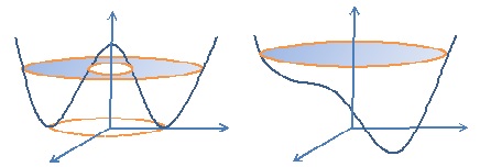
Figure 1: Graphs and level sets of $G({\bf x})$ for ${{\mbox{\boldmath$\tau$}}}=0$ (left) and ${{\mbox{\boldmath$\tau$}}}\neq 0$ (right)

Fig. 1 shows that although $G(\mbox{\boldmath$\gamma$})$ has only one global minimizer for certain given $\tau$, the function is still nonconvex. Such a function is called quasiconvex in the context of global optimization. In order to distinguish this type of functions with Morry’s quasiconvexity in nonconvex analysis, a generalized definition in a tensor space ${\cal{F}}_{a}\subset\mathbb{R}^{m\times n}$ could be convenient.

Definition 1 (G-Quasiconvexity)

A function $G:{\cal{F}}_{a}\subset\mathbb{R}^{m\times n}\rightarrow\mathbb{R}$ is called G-quasiconvex if its domain ${\cal{F}}_{a}$ is convex and

$$G(\theta{\bf F}+(1-\theta){\bf T})\leq\max\{G({\bf F}),G({\bf T})\}\;\;\forall{\bf F},\;{\bf T}\in{\cal{F}}_{a},\;\;\forall\theta\in[0,1].$$ (44)

It is called strictly G-quasiconvex if the inequality holds strictly.

Moreover, we may need a definition of generalize ellipticity for nonconvex systems.

Definition 2 (G-Ellipticity)

For a given function $G:{\cal{F}}_{a}\rightarrow\mathbb{R}$ and $\alpha\in\mathbb{R}$, its level set ${\cal L}_{\alpha}(G)$ is said to be a G-ellipse if it is a closed, simply connected set. For a given ${\bf t}$ such that ${\bf T}\in{\cal{T}}_{a}$, the $(BVP)$ is said to be $G$-elliptic if the total potential function $G({\bf F})$ is G-quasiconvex on ${\cal{F}}_{a}$. $(BVP)$ is strongly G-elliptic if $G({\bf F})$ is strictly G-quasiconvex.

Lemma 1

For a given function $G:{\cal{F}}_{a}\subset\mathbb{R}^{m\times n}\rightarrow\mathbb{R}$,

$$G({\bf F}) \Leftrightarrow {\cal L}^{\flat}_{\alpha}(G) \Leftrightarrow {\cal L}_{\alpha}(G) \forall\alpha\in\mathbb{R}$$ is G-quasiconvex is convex is a G-ellipse . (45)

$$\mbox{ $G({\bf F})$ is convex $\Rightarrow$ is rank-one convex $\Rightarrow$ G-quasiconvex $\Rightarrow$ $(BVP)$ is G-elliptic}.$$ (46)

This statement shows an important fact in nonconvex systems, i.e. the total number of solutions to a nonlinear equation depends not only on the stored energy, but also (mainly) on the external force field. The nonlinear partial differential equation in $(BVP)$ is elliptic only if it is G-elliptic. $(BVP)$ has at most one solution if $G({\bf F})$ is strictly G-quasiconvex on ${\cal{F}}_{a}$.

Remark 3 (Existence and Uniqueness)

Suppose that the canonical function $V:{\cal{E}}_{a}\rightarrow\mathbb{R}$ is convex, then $\nabla V^{*}(\zeta)>0$ is a monotonic operator on ${\cal{E}}^{*}_{a}$. If for any given ${\bf t}:{S_{t}}\rightarrow\mathbb{R}^{3}$ such that ${\bf T}\in{\cal{T}}_{a}\neq\emptyset$ and $\tau^{2}({\bf x})=\mbox{tr\hskip 1.0pt}({\bf T}^{T}{\bf T})\neq 0\;\;\forall{\bf x}\in{\cal B}$, then the nonconvex variational problem $({\cal P})$ has at least one nontrivial solution a.e. in ${\cal B}$. It has a unique nontrivial solution if there exists a constant $\tau_{c}$ such that $\tau^{2}({\bf x})=\mbox{tr\hskip 1.0pt}({\bf T}^{T}{\bf T})\geq\tau_{c}^{2}\;\;\forall{\bf x}\in{\cal B}$.

In global optimization, the most simple quadratic integer programming problem

$$({\cal P})_{i}:\;\;\;\min\left\{\Pi({\bf x})=\frac{1}{2}{\bf x}^{T}{\bf Q}{\bf x}-{\bf x}^{T}{\bf t}\;\;|\;\;{\bf x}=\{x_{i}\}^{n}\in\{0,1\}^{n}\subset\mathbb{R}^{n}\right\}$$

could have up to $2^{n}$ local minimizers, which can’t be solved directly by traditional deterministic methods in polynomial time due to the indefinite matrix ${\bf Q}$ and the integer constraint. Such a nonconvex discrete optimization problem is considered as NP-hard in computer science. However, by using canonical transformation $\mbox{\boldmath$\xi$}=\Lambda({\bf x})=\{x_{i}(x_{i}-1)\}\in\mathbb{R}^{n}$, the canonical dual of this discrete problem is a concave maximization over a convex set in continuous space [12]. It was proved in [7] that there exists a positive vector ${\mbox{\boldmath$\tau$}}=\{\tau_{i}\}^{n}>{\bf 0}\in\mathbb{R}^{n}$, if $\{|t_{i}|\leq\tau_{i}\}^{n}$, then ${\cal{S}}^{+}_{a}\neq\emptyset$ and $({\cal P})_{i}$ is not NP-hard. The decision variable is simply $\{x_{i}\}=\{0\mbox{ if }t_{i}<-\tau_{i},\;1\;\mbox{ if }t_{i}>\tau_{i}\}$ (Theorem 8, [7]). Thus, the canonical duality theory can be used to identify NP-hard problems [12].

4 Applications in Anti-Plane Shear Deformation

Now let us consider a special case that the homogeneous elastic body ${\cal B}\subset\mathbb{R}^{3}$ is a cylinder with generators parallel to the ${\bf e}_{3}$ axis and with cross section a sufficiently nice region $\Omega\subset\mathbb{R}^{2}$ in the ${\bf e}_{1}\times{\bf e}_{2}$ plane. The so-called anti-plane shear deformation is defined by (see [14])

$$\mbox{\boldmath$\chi$}({\bf x})=\left\{x_{1},\;\;x_{2},\;\;x_{3}+{u}({x}_{1},{x}_{2})\right\}:\Omega\subset\mathbb{R}^{2}\rightarrow\mathbb{R}^{3},$$ (47)

where $({x}_{1},{x}_{2},{x}_{3})$ are cylindrical coordinates in the reference configuration ${\cal B}$ relative to a cylindrical basis $\{{\bf e}_{i}\},\;i=1,2,3$. On ${\Gamma_{\chi}}\subset\partial\Omega$, the homogenous boundary condition is given ${u}(x_{\alpha})=0\;\;\forall x_{\alpha}\in{\Gamma_{\chi}},\;\;\alpha=1,2.$ On the remaining boundary ${\Gamma_{t}}=\partial\Omega\cap{\Gamma_{\chi}}$, the cylinder is subjected to the shear force

$${\bf t}({\bf x})=t({\bf x}){\bf e}_{3}\;\;\forall{\bf x}\in{\Gamma_{t}},$$

where $t:{\Gamma_{t}}\rightarrow\mathbb{R}$ is a prescribed function. For this anti-plane shear deformation we have

$$\mathbf{F}=\nabla\mbox{\boldmath$\chi$}=\left(\begin{array}[]{ccc}1&0&0\\ 0&1&0\\ {u}_{,1}&{u}_{,2}&1\end{array}\right),\;\;\;\;\mathbf{C}=\mathbf{F}^{\rm T}{\bf F}=\left(\begin{array}[]{ccc}1+{u}_{,1}^{2}&{u}_{,1}{u}_{,2}&{u}_{,1}\\ {u}_{,1}{u}_{,2}&1+{u}_{,2}^{2}&{u}_{,2}\\ {u}_{,1}&{u}_{,2}&1\end{array}\right),$$ (48)

where ${u}_{,\alpha}$ represents $\partial{u}/\partial x_{\alpha}$ for $\alpha=1,2$. By the notation $|\nabla{u}|^{2}={u}_{,1}^{2}+{u}_{,2}^{2}$, we have

$$I_{1}({\bf C})=I_{2}({\bf C})=3+|\nabla{u}|^{2},\;\;I_{3}({\bf C})\equiv 1,$$ (49)

Clearly, both ${\bf F}$ and $I_{1}({\bf C})$ depend only on the shear strain $\mbox{\boldmath$\gamma$}=\nabla{u}=\{{u}_{,\alpha}\}$, therefore, the strain energy can be equivalently written in the forms of

$${W}({\bf F}(\mbox{\boldmath$\gamma$}))=V(\xi(\mbox{\boldmath$\gamma$}))=\hat{W}(\mbox{\boldmath$\gamma$})$$ (50)

where $\hat{W}(\mbox{\boldmath$\gamma$})$ is a real-valued function.

The fact $\det{\bf F}\equiv 1$ shows that the anti-plane shear state (47) is an isochoric deformation. Therefore, the kinetically admissible displacement space ${\cal{X}}_{c}$ can be simply replaced by a convex set

$${\cal{U}}_{c}=\{{u}({\bf x})\in{\cal W}^{1,1}(\Omega;\mathbb{R})|\;\;{u}({\bf x})=0\;\;\forall{\bf x}=\{x_{\alpha}\}\in{\Gamma_{\chi}}\}.$$ (51)

Thus, in terms of $\xi=\Lambda(\mbox{\boldmath$\gamma$})=I_{1}-3=|\mbox{\boldmath$\gamma$}|^{2}$ and ${W}({\bf F}(\mbox{\boldmath$\gamma$}))=V(\Lambda(\mbox{\boldmath$\gamma$}))$, for any given

$${\mbox{\boldmath$\tau$}}\in{\cal{T}}_{a}=\{{\mbox{\boldmath$\tau$}}\in C^{1}[\Omega;\mathbb{R}^{2}]|\;\;\nabla\cdot{\mbox{\boldmath$\tau$}}=0\;\;\mbox{ in }\Omega,\;\;{\bf n}\cdot{\mbox{\boldmath$\tau$}}=t\;\;\mbox{ on }{\Gamma_{t}}\}$$

Problem $({\cal P})_{{\bf T}}$ for the anti-plane shear deformation (47) has the following form

$$({\cal P})_{s}:\;\;\min\left\{\Pi({u})=\int_{\Omega}G(\nabla{u}){\rm d}\Omega\;\;|\;\;{u}\in{\cal{U}}_{c}\right\},\;\;G(\mbox{\boldmath$\gamma$})=V(\Lambda(\mbox{\boldmath$\gamma$}))-\mbox{\boldmath$\gamma$}^{T}{\mbox{\boldmath$\tau$}}$$ (52)

Under certain regularity conditions, the associated mixed boundary value problem is

$$(BVP)_{s}:\;\;\left\{\begin{array}[]{l}\nabla\cdot\left(2\zeta\nabla{u}\right)=0\;\;\mbox{ in }\Omega,\\ {\bf n}\cdot\left(2\zeta\nabla{u}\right)=t\;\;\mbox{ on }{\Gamma_{t}},\;\;{u}=0\;\;\mbox{ on }{\Gamma_{\chi}}\end{array}\right.$$ (53)

where ${\bf n}=\{n_{\alpha}\}\in\mathbb{R}^{2}$ is a unit vector norm to $\partial\Omega$, and $\zeta=\nabla V(\xi),\;\;\xi=|\nabla{u}|^{2}$.

If ${\Gamma_{\chi}}=\partial\Omega$, then $(BVP)_{s}$ is a Dirichlet boundary value problem, which has only trivial solution due to zero input. For Neumann boundary value problem ${\Gamma_{t}}=\partial\Omega$, the external force field must be such that

$$\int_{\Gamma_{t}}t({\bf x}){\rm d}\Gamma=0$$

for overall force equilibrium. In this case, if $\bar{\mbox{\boldmath$\chi$}}$ is a solution to $(BVP)_{s}$, then $\mbox{\boldmath$\chi$}=\bar{\mbox{\boldmath$\chi$}}+{\bf c}$ is also a solution for any vector ${\bf c}\in\mathbb{R}^{3}$ since the cylinder is not fixed. Therefore, the mixed boundary value problem $(BVP)_{s}$ is necessary for anti-plane shear deformation to have a unique solution.

By the fact that the only unknown ${u}$ is a scalar-valued function, anti-plane shear deformations are one of the simplest classes of deformations that solids can undergo [14]. Indeed, if $V(\xi)$ is a canonical function on ${\cal{E}}_{a}=\{\xi\in L^{p}(\Omega)|\;\;\xi({\bf x})\geq 0\;\;\forall{\bf x}\in\Omega\}$ and for any given ${\mbox{\boldmath$\tau$}}\in{\cal{T}}_{a}$ such that $\tau=|{\mbox{\boldmath$\tau$}}|$, the canonical dual problem has a very simple form

$$({\cal P}^{d})_{s}:\;\;\;\;{\rm sta}\left\{\Pi^{d}(\zeta)=\int_{\Omega}\left[-V^{*}(\zeta)-\frac{1}{4}\zeta^{-1}\tau^{2}\right]{\rm d}\Omega\;|\;\;\zeta\in{\cal{S}}_{a}\right\}.$$ (54)

Since $\Lambda({u})=|\nabla{u}|^{2}$, the canonical dual algebraic equation (24) for this problem is

$$4\zeta^{2}\nabla V^{*}(\zeta)=\tau^{2}({\bf x}),\;\;\;\;\forall{\bf x}\in\Omega.$$ (55)

Corollary 1

For any given non-trivial shear force $t({\bf x})\neq 0$ on ${\Gamma_{t}}$ such that ${\mbox{\boldmath$\tau$}}\in{\cal{T}}_{a}\neq\emptyset$, the canonical dual problem $({\cal P}^{d})_{s}$ has at least one non-trivial solution $\zeta_{k}$. If $\nabla\times\zeta_{k}^{-1}{\mbox{\boldmath$\tau$}}=0$, the scale-valued function

$${u}_{k}({\bf x})=\frac{1}{2}\int_{{\bf x}_{0}}^{\bf x}\zeta_{k}^{-1}{\mbox{\boldmath$\tau$}}\cdot\mbox{d}{\bf x}$$ (56)

along any path from ${\bf x}_{0}\in{\Gamma_{\chi}}$ to ${\bf x}\in\Omega$ is a critical point of $\Pi({u})$ and $\Pi({u}_{k})=\Pi^{d}(\zeta_{k})$.

If $\zeta_{k}\in{\cal{S}}^{+}_{a}$, then ${u}_{k}$ is a global minimizer of $({\cal P})_{s}$.

If $\zeta_{k}\in{\cal{S}}^{-}_{a}$ and ${\bf G}(\zeta_{k})\succ 0$, then ${u}_{k}$ is a local minimizer of $({\cal P})_{s}$.

If $\zeta_{k}\in{\cal{S}}^{-}_{a}$ and ${\bf G}(\zeta_{k})\prec 0$, then ${u}_{k}$ is a local maximizer of $({\cal P})_{s}$.

Example. Applications of the canonical duality theory to general anti-plane shear problems have been demonstrated for solving convex exponential and nonconvex polynomial stored energies recently in [8]. In this paper, the following generalized neo-Hookean model is considered

$$V(\xi)={c}_{1}(I_{1}-3)+{c}_{2}(I_{1}-3)\log(I_{1}-3)$$ (57)

where ${c}_{1},\;{c}_{2}$ are positive material constants. Clearly, $V(\xi)$ is convex in $\xi=I_{1}-3$, but

$$\hat{W}(\mbox{\boldmath$\gamma$})=V(I_{1}(\mbox{\boldmath$\gamma$}))={c}_{1}|\mbox{\boldmath$\gamma$}|^{2}+{c}_{2}|\mbox{\boldmath$\gamma$}|^{2}\log|\mbox{\boldmath$\gamma$}|^{2}$$

is a double-well function of the shear strain $\mbox{\boldmath$\gamma$}=\nabla{u}$ (see Fig. 2).

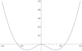
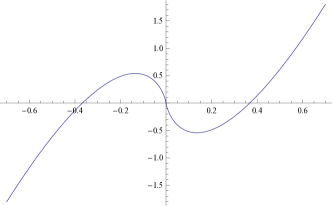
(a)

Figure 2: Graphs of $\hat{W}(\mbox{\boldmath$\gamma$})$ (a) and its derivative (b) (${c}_{1}={c}_{2}=1$)

It is easy to check

$$\zeta=\nabla V(\xi)={c}_{1}+{c}_{2}(\log\xi+1):{\cal{E}}_{a}\rightarrow{\cal{E}}_{a}^{*}=L^{q}(\Omega)$$

is one-to-one and onto, where $q$ is a dual number of $p\geq 1$, i.e. $1/p+1/q=1$. The complementary energy can be obtained easily

$$V^{*}(\zeta)={\rm sta}\{\xi\zeta-V(\xi)|\;\;\xi\in{\cal{E}}_{a}\}={c}_{2}\exp[{c}_{2}^{-1}(\zeta-{c}_{1})-1]$$

In this case, the canonical dual algebraic equation is

$$\zeta^{2}\exp\left[\frac{\zeta-{c}_{1}}{{c}_{2}}-1\right]=\tau^{2}({\bf x})\;\;\forall{\bf x}\in\Omega.$$ (58)

Let $h^{2}(\zeta)=\zeta^{2}\exp[(\zeta-{c}_{1})/{c}_{2}-1]$ be the left hand side function in the canonical dual algebraic equation (58). By solving $h^{\prime}(\zeta_{c})=0$ we known that at $\zeta_{c}=-2{c}_{2}$, $h(\zeta)$ has a local maximum

$$h_{\max}(\zeta_{c})=\eta=2{c}_{2}\sqrt{\exp[-3-{c}_{1}/{c}_{2}]}.$$

From the graphs of the canonical dual algebraic curve $h(\zeta)$ given in Fig. 3 we can see that the canonical dual algebraic equation (58) may have at most three real solutions in the order of $\zeta_{1}\geq 0\geq\zeta_{2}\geq\zeta_{3}$ depending on $\tau=|{\mbox{\boldmath$\tau$}}({\bf x})|,\;\;{\bf x}\in\Omega$ (see Fig. 3b). The equation (58) has a unique solution if $\tau>\eta$. In this case, the total strain grand $G(\gamma)$ is strictly G-quasiconvex (see Fig. 4). Fig 5 shows the graphs of $G(\gamma)$ and its canonical dual $G^{d}(\zeta)$ for $\tau<\eta$. In this case, the function $G(\gamma)$ is nonconvex and has three critical points. The triality theory holds for $G(\gamma)$ and its canoncial dual $G^{d}(\zeta)$

$$G(\gamma_{1})=\min_{\gamma\geq 0}G(\gamma)=\max_{\zeta>0}G^{d}(\zeta)=G^{d}(\zeta_{1}).$$

$$G(\gamma_{2})=\min_{\gamma\in{\cal{G}}_{o}}G(\gamma)=\min_{\zeta>-2{c}_{2}}G^{d}(\zeta)=G^{d}(\zeta_{2}).$$

$$G(\gamma_{3})=\max_{\gamma\in{\cal{G}}_{o}}G(\gamma)=\max_{\zeta<-2{c}_{2}}G^{d}(\zeta)=G^{d}(\zeta_{3}),$$

where ${\cal{G}}_{o}$ is a neighborhood of $\gamma_{i}$ $(i=1,2)$.

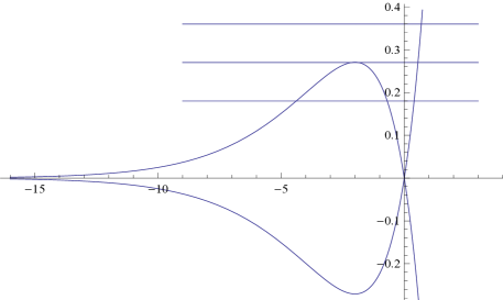
Figure 3: Dual algebraic curve $h(\zeta)\;({c}_{1}={c}_{2}=1)$

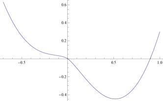
(a) $\tau>\eta$

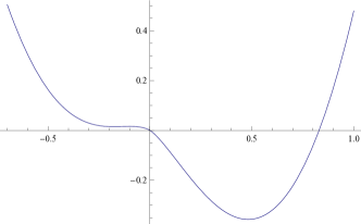
(b) $\tau=\eta$

Figure 4: Graphs of G-quasiconvex $G(\gamma)$ (${c}_{1}={c}_{2}=1$)

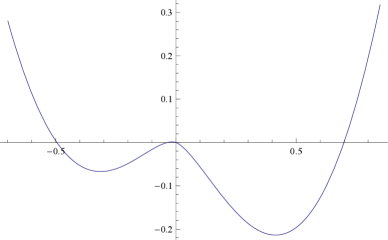
(a) Graph of $G(\gamma)$

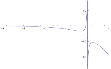
(b) Graph of $G^{d}(\zeta)$

Figure 5: Graphs of $G(\gamma)$ and $G^{d}(\zeta)$ for $\tau<\eta$ (${c}_{1}={c}_{2}=1$ )

5 Conclusions

In summary, the following conclusions can be obtained.

1. The pure complementary energy principle and canonical duality-triality theory developed in [6] are useful for solving general nonlinear boundary value problems in nonlinear elasticity.

2. Both convexity of the total potential and ellipticity condition of the associated fully nonlinear boundary value problem depend not only on the stored energy function, but also sensitively on the external force field.

3. The Legendre-Hadamard condition is only a necessary ellipticity condition for convex systems. The triality theory provides a sufficient condition to identify both global and local extremum solutions for nonconvex problems.

These conclusions are naturally included in the canonical duality-triality theory developed by the author and his co-workers during the last 25 years [6]. Extensive applications have been given in multidisciplinary fields of biology, chaotic dynamics, computational mechanics, information theory, phase transitions, post-buckling, operations research, industrial and systems engineering, etc. (see recent review article [12]).

Acknowledgements

Insightful discussions with Professor David Steigmann from UC-Berkeley is sincerely acknowledged. The research was supported by US Air Force Office of Scientific Research (AFOSR FA9550-10-1-0487).

References

[1]
[2]Ciarlet, P.G. (2013). Linear and Nonlinear Functional Analysis with Applications, SIAM, Philadelphia.
[3] Gao, D.Y. (1992).
Global extremum criteria for nonlinear elasticity,
ZAMP, 43, pp. 924-937.
[4] Gao, D.Y. (1998).
Duality, triality and complementary extremum principles in nonconvex parametric variational problems with applications
IMAJ. Appl. Math. 61, pp. 199-235.
[5] Gao, D.Y. (1999). General analytic solutions and
complementary variational principles for large deformation nonsmooth mechanics. Meccanica 34, 169-198.
[6] Gao, D.Y. (2000). Duality Principles in Nonconvex
Systems: Theory, Methods and Applications, Kluwer Academic
Publishers, Dordrecht /Boston /London, xviii + 454pp.
[7] Gao, D.Y. (2009).
Canonical duality theory: unified understanding and generalized solutions for
global optimization. Comput. & Chem. Eng. 33,
1964-1972.
[8]Gao, D.Y. (2015)
Analytical solutions to general anti-plane shear problem in finite elasticity.
Continuum Mech Theorm. , 2015.
[9]Gao, DY and Hajilarov, E. (2015). Analytic solutions to three-dimensional
finite deformation problems governed by
St Venant Kirchhoff material, Math Mech Solids, DOI: 10.1177/1081286515591084
[10] Gao, D.Y. and Ogden, R.W. (2008).
Closed-form solutions, extremality and nonsmoothness criteria in a large deformation elasticity problem,
ZAMP, 59:498 - 517.
[11] Gao, D.Y. and Ogden, R.W. (2008).
Multiple solutions to non-convex variational problems with implications for phase transitions and numerical computation, Quarterly J. Mech. Appl. Math. 61 (4), 497-522.
[12] Gao, DY, Ruan, N, and Latorre, V (2015).
Canonical duality-triality: Bridge between nonconvex analysis/mechanics and global optimization in complex systems.
Math. Mech. Solids.
[13] Gao, D.Y. and Strang, G. (1989).
Geometric nonlinearity: Potential energy, complementary energy, and the gap function,
Quart. Appl. Math., 47, pp. 487-504.
[14] Horgan, C.O. (1995).
Anti-Plane Shear Deformations in Linear and Nonlinear Solid Mechanics,
SIAM Review, 37(1), 53-81.
[15] Li, S.F. and Gupta, A. (2006). On dual configuration forces,
J. of Elasticity, 84:13-31.
[16] Martin, RJ, Ghiba, I-D, and Neff, P. (2015).
Rank-one convexity implies polyconvexity for isotropic,
objective and isochoric elastic energies in the
two-dimensional case. http://www.researchgate.net/publication/279632850
[17] Morrey, C.B. (1966). Multiple Integrals in the Calculus of Variations, Springer, Berlin.