Conjugate Gradient Acceleration of
Non-Linear Smoothing Filters

Abstract

The most efficient signal edge-preserving smoothing filters, e.g., for denoising, are non-linear. Thus, their acceleration is challenging and is often performed in practice by tuning filter parameters, such as by increasing the width of the local smoothing neighborhood, resulting in more aggressive smoothing of a single sweep at the cost of increased edge blurring. We propose an alternative technology, accelerating the original filters without tuning, by running them through a special conjugate gradient method, not affecting their quality. The filter non-linearity is dealt with by careful freezing and restarting. Our initial numerical experiments on toy one-dimensional signals demonstrate 20x acceleration of the classical bilateral filter and 3-5x acceleration of the recently developed guided filter.

I Introduction

This paper is concerned with noise removal from a given noisy signal, which is a basic problem in signal processing, with many applications, e.g., in image denoising [6]. Modern denoising algorithms preserve signal details while removing most of the noise. A very popular denoising filter is the bilateral filter (BF), which smooths signals while preserving edges, by taking the weighted average of the nearby pixels. The weights depend on both the spatial distance between the sampling locations and similarity between signal values, thus providing local adaptivity to the input signal. Bilateral filtering has initially been proposed in [12] as an intuitive tool without theoretical justification. Since then, connections between BF and other well-known filtering techniques such as anisotropic diffusion, weighted least squares, Bayesian methods, kernel regression and non-local means have been explored; see, e.g., survey [13].

We make use of the graph-based framework for signal analysis developed in [5, 7], where polynomial low-pass filters based on the BF coefficients are proposed. A nice introduction to signal processing on graphs is found in [2].

A single application of BF can be interpreted as a vertex domain transform on a graph with pixels as vertices, intensity values of each node as the graph signal, and filter coefficients as link weights that capture the similarity between nodes. The BF transform is a special nonlinear anisotropic diffusion, cf. [9, 10], determined by the entries of the graph Laplacian matrix, which are related to the BF weights. The eigenvectors and eigenvalues of the graph Laplacian matrix allow us to extend the Fourier analysis to the graph signals or images as in [2] and perform frequency selective filtering operations on graphs, similar to those in traditional signal processing.

Another very interesting smoothing filter is the guided filter (GF), recently proposed in [11, 3], and included into the MATLAB image processing toolbox. Some ideas behind GF are developed in [4]. According to our limited experience, GF is faster than BF. The authors of [11] advocate that GF is gradient preserving and avoids gradient reversal artifacts in contrast to BF, which is not gradient preserving.

The smoothing explicit filters similar to BF and GF can be interpreted as matrix power iterations, which are, in general case, nonlinear, or equivalently, as explicit integration in time of the corresponding nonlinear anisotropic diffusion equation [9, 10]. The suitable graph Laplacian matrices are determined by means of the graph-based interpretation of these power iterations. Our main contribution is accelerating the smoothing filters by means of a special variant of the conjugate gradient (CG) method, applied to the corresponding graph Laplacian matrices. To avoid oversmoothing, only few iterations of the CG acceleration can be performed. We note that there exist several nonlinear variants of the CG algorithm, see, e.g., [8]. However, the developed theory is not directly applicable in our case because it is not clear how to interpret the vector $L(x)x$ as a gradient of a scalar function of the signal $x$, where $L(x)$ is a graph Laplacian matrix depending on a signal $x$.

II Bilateral filter (BF)

We consider discrete signals defined on an undirected graph $\mathcal{G}=(\mathcal{V},\mathcal{E})$, where the vertices $\mathcal{V}=\{1,2,\ldots,N\}$ denote, e.g., time instances of a discrete-time signal or pixels of an image. The set of edges $\mathcal{E}=\{(i,j)\}$ contains only those pairs of vertices $i$ and $j$ that are neighbors in some predefined sense. We suppose in addition that a spatial position $p_{i}$ is assigned to each vertex $i\in\mathcal{V}$ so that a distance $\|p_{i}-p_{j}\|$ is determined between vertices $i$ and $j$.

Let $x[j]$, $j\in\mathcal{V}$, be a discrete function, which is an input signal to the bilateral filter. The output signal $y[i]$ is the weighted average of the signal values in $x[j]$:

$$y[i]=\sum_{j}\frac{w_{ij}}{\sum_{j}w_{ij}}x[j].$$ (1)

The weights $w_{ij}$ are defined for $(i,j)\in\mathcal{E}$ in terms of a guidance signal $g[i]$:

$$w_{ij}=\exp\left(-\frac{\|p_{i}-p_{j}\|^{2}}{2\sigma_{d}^{2}}\right)\exp\left(-\frac{(g[i]-g[j])^{2}}{2\sigma_{r}^{2}}\right),$$ (2)

where $\sigma_{d}$ and $\sigma_{r}$ are the filter parameters [12]. The guidance signal $g[i]$ is chosen depending on the purpose of filtering. When $g$ coincides with the input $x$, the bilateral filter is nonlinear and called self-guided.

The weights $w_{ij}$ determine the adjacency matrix $W$ of the graph $G$. The matrix $W$ is symmetric, has nonnegative elements and diagonal elements equal to 1. Let $D$ be the diagonal matrix with the nonnegative diagonal entries $d_{i}=\sum_{j}w_{ij}$. Thus, the BF operation (1) is the vector transform defined by the aid of the matrices $W(g)$ and $D(g)$ as $y=D^{-1}Wx=x-D^{-1}Lx$, where $L=D-W$ is called the Laplacian matrix of the weighted graph $G$ with the BF weights. The eigenvalues of the matrix $D^{-1}W$ are real. The eigenvalues corresponding to the highest oscillations lie near the origin.

The BF transform $y=D^{-1}Wx$ can be applied iteratively, (i) by changing the weights $w_{ij}$ at each iteration using the result of the previous iteration as a guidance signal $g$, or (ii) by using the fixed weights, calculated from the initial signal as a guidance signal, for all iterations. The former alternative results in a nonlinear filter. The latter produces a linear filter, which may be faster, since the BF weights are computed only once in the very beginning.

An iterative application of the BF matrix transform is the power iteration with the amplification matrix $D^{-1}W$. Slow convergence of the power iteration can be boosted by the aid of suitable Krylov subspace iterative methods [1, 14].

III Guided filter (GF)

Algorithm 1 Guided Filter (GF)
Input: $x$, $g$, $\rho$, $\epsilon$
Output: $y$
$mean_{g}=f_{mean}(g,\rho)$
$mean_{x}=f_{mean}(x,\rho)$
$corr_{g}=f_{mean}(g.*g,\rho)$
$corr_{gx}=f_{mean}(g.*x,\rho)$
$var_{g}=corr_{g}-mean_{g}.*mean_{g}$
$cov_{gx}=corr_{gx}-mean_{g}.*mean_{x}$
$a=cov_{gx}./(var_{g}+\epsilon)$
$b=mean_{x}-a.*mean_{g}$
$mean_{a}=f_{mean}(a,\rho)$
$mean_{b}=f_{mean}(b,\rho)$
$y=mean_{a}.*g+mean_{b}$

Algorithm 1 is a pseudo-code of GF proposed in [11], where $x$ and $y$ are, respectively, the input and output signals on the graph $G$, described in section II. GF is built by means of a guidance signal $g$, which equals $x$ in the self-guided case. The function $f_{mean}(\cdot,\rho)$ denotes a mean filter of a spatial radius $\rho$. The constant $\epsilon$ determines the smoothness degree of the filter—the larger $\epsilon$ the larger smoothing effect. The dot preceded operations $.*$ and $./$ denote the componentwise multiplication and division. A typical arithmetical complexity of the GF algorithm is $O(N)$, where $N$ is the number of elements in $x$, see [11].

The guided filter operation of Algorithm 1 is the matrix transform $y=W(g)x$, where the implicitly constructed transform matrix $W(g)$ has the following entries, see [11]:

$$W_{ij}(g)=\frac{1}{|\omega|^{2}}\sum_{k\colon(i,j)\in\omega_{k}}\left(1+\frac{(g_{i}-\mu_{k})(g_{j}-\mu_{k})}{\sigma_{k}^{2}+\epsilon}\right).$$ (3)

The mean filter $f_{mean}(\cdot,\rho)$ is applied in the neighborhoods $\omega_{k}$ of a spatial radius $\rho$ around all vertices $k\in\mathcal{V}$. The number of pixels in $\omega_{k}$ is denoted by $|\omega|$, the same for all $k$. The values $\mu_{k}$ and $\sigma_{k}^{2}$ are the mean and variance of $g$ over $\omega_{k}$. The matrix $W$ is symmetric and satisfies the property $\sum_{j}W_{ij}=1$.

The standard construction of the graph Laplacian matrix gives $L=I-W$, because $d_{i}=\sum_{j}w_{ij}=1$, i.e. the matrix $D$ is the identity. The eigenvalues of $L(g)$ are real nonnegative with the low frequencies accumulated near 0 and high frequencies near 1. Application of a single transform $y=Wx$ attenuates the high frequency modes of $x$ while approximately preserving the low frequency modes, cf. [7, 5]. Similar to the BF filter, the guided filter can be applied iteratively. When the guidance signal $g$ is fixed, the iterated GF filter is linear. When $g$ varies, for example, $g=x$ for the self-guided case, the iterated GF filter is nonlinear.

IV Conjugate gradient acceleration

Since the graph Laplacian matrix $L$ is symmetric and nonnegative definite, the iterative application of the transform $y=D^{-1}Wx$ can be accelerated by adopting by the CG technology. We use two variants of CG: 1) with the fixed guidance equal to the input signal or to the clean signal, 2) with the varying guidance equal to the current value of $x$.

Algorithm 2 Truncated PCG($k_{\max}$)

Input: $x_{0}$, $g$, $k_{\max}$ Output: $x$

$x=x_{0}$; $r=W(g)x-D(g)x$

for $k=1,\ldots,k_{\max}-1$ do

$s=D^{-1}(g)r$; $\gamma=s^{T}r$

if $k=1$ then $p=s$ else $\beta=\gamma/\gamma_{old}$; $p=s+\beta p$

endif

$q=D(g)p-W(g)p$; $\alpha=\gamma/(p^{T}q)$

$x=x+\alpha p$; $r=r-\alpha q$; $\gamma_{old}=\gamma$

endfor

Algorithm 2 is the standard preconditioned conjugate gradient algorithm formally applied to the system of linear equations $Lx=0$ and truncated after $k_{\max}$ evaluations of the matrix-vector operation $Lx$. The initial vector $x_{0}$ is a noisy input signal. This variant of the CG algorithm has first been suggested in [5].

Algorithm 3 is a special nonlinear preconditioned CG with $l_{\max}$ restarts, formally applied to $L(x)x=0$ and truncated after $k_{\max}$ iterations between restarts. Restarts are necessary because of nonlinearity of the self-guided filtering.

Algorithm 3 Truncated PCG($k_{\max}$) with $l_{\max}$ restarts

Input: $x_{0}$, $k_{\max}$, $l_{max}$ Output: $x$

$x=x_{0}$

for $l=1,\ldots,l_{\max}$ do

$r=W(x)x-D(x)x$

for $k=1,\ldots,k_{\max}-1$ do

$s=D^{-1}(x)r$; $\gamma=s^{T}r$

if $k=1$ then $p=s$ else $\beta=\gamma/\gamma_{old}$; $p=s+\beta p$

endif

$q=D(x)p-W(x)p$; $\alpha=\gamma/(p^{T}q)$

$x=x+\alpha p$; $r=r-\alpha q$; $\gamma_{old}=\gamma$

endfor

endfor

V Numerical experiments

As a proof of concept, our MATLAB tests use the clean 1-dimensional signal $x_{c}$ of length $N=4730$ shown in Figure 1. We choose this rather difficult, although 1-dimensional, example to better visually illustrate both the denoising and edge-preserving features of the filters. The noisy signal, also displayed in Figure 1, is the same for all tests and given by the formula $x_{0}=x_{c}+\eta$, where a Gaussian white noise $\eta$ has zero mean and variance $\sigma^{2}=0.01$. The bilateral filter is used with $\sigma_{d}=0.5$ and $\sigma_{r}=0.1$. The neighborhood width in BF equals 5 so that the band of $W$ consists of 5 diagonals. The guided filter is used with $\epsilon=0.001$ and the neighborhood width 3. The matrix $W$ of GF also has 5 diagonals.

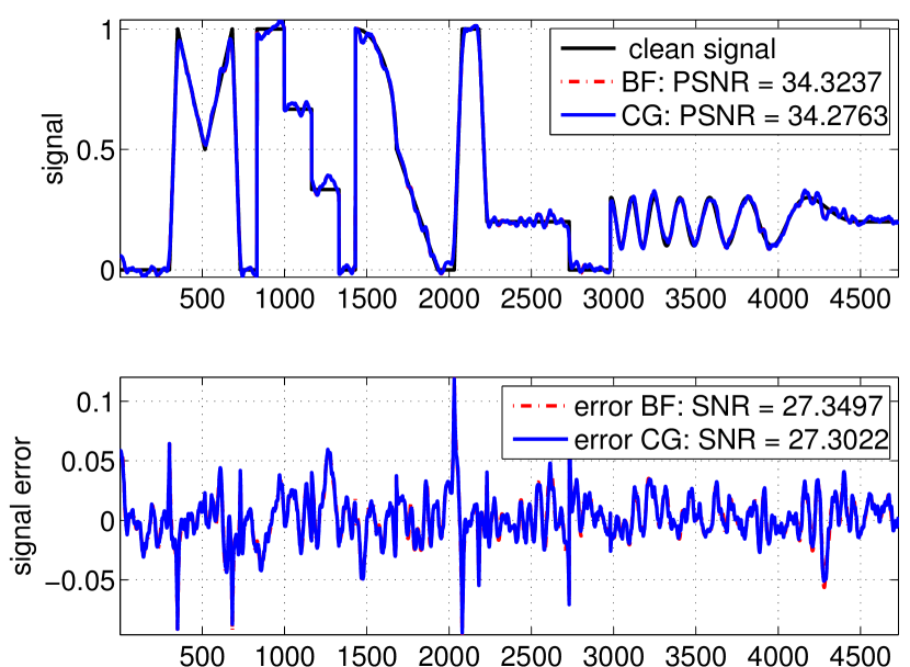
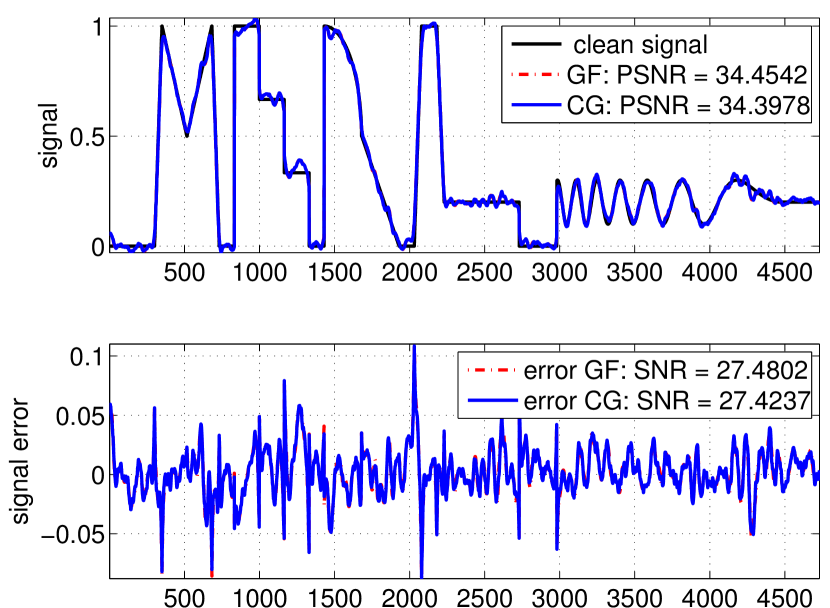
The CG accelerated BF/GF is called CG-BF/CG-GF. Typical numerical results of the average performance are displayed.

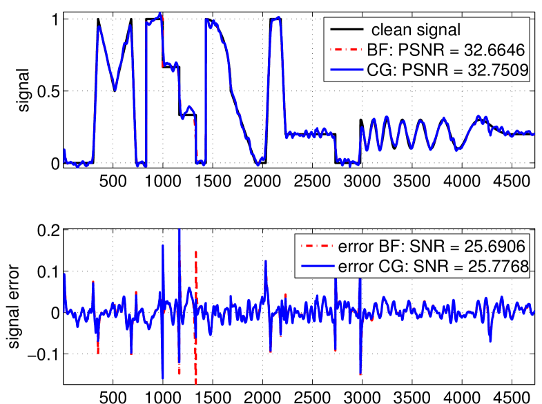
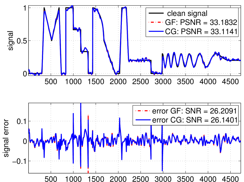
The signal error after denoising is $\widehat{x}-x_{0}$, where $\widehat{x}$ stands for the output denoised signal. We calculate the peak signal-to-noise ratio (PSNR) and signal-to-noise ration (SNR). The parameters are manually optimized to reach the best possible match of the signal errors in the compared filters, resulting in indistinguishable error curves in our figures.

The results in Figures 2 and 3 are obtained by the iterated BF and GF filters with the fixed guidance $g=x_{c}$ and by CG-BF and CG-GF implemented in Algorithm 2 with the same fixed guidance $g=x_{c}$. These tests are performed only for comparison reasons because the clean signal guidance $x_{c}$ seems to be ideal for the best possible denoising results.

We say that Algorithm 3 uses $l_{\max}\times k_{\max}$ iterations, if it executes $l_{\max}$ restarts with the $k_{\max}$ evaluations $L(x)x$ between restarts. The best denoising performance for our test problem is achieved with the following iteration combinations of the self-guided CG-BF: $31\times 3$, $17\times 4$, $12\times 5$, $9\times 6$, $7\times 7$, $6\times 8$, $5\times 9$, $4\times 10$, $3\times 11$, $2\times 19$. The best combinations for the self-guided CG-GF are $11\times 3$, $7\times 4$, $5\times 5$, $4\times 6$, $3\times 7$. Figures 4 and 5 show the results after $3\times 11$ iterations of CG-BF and $5\times 5$ iterations of CG-GF.

The numerical tests demonstrate about $20$-times reduction of iterations for the self-guided bilateral filter and $3$-times reduction of iterations for the guided filter with self-guidance after the conjugate gradient acceleration. It is also interesting to observe that both filters with the properly chosen parameters and iteration numbers produce almost identical output signals.

Figure 1: Clean and noisy signals.

Figure 2: 500 BF iterations versus 20 CG-BF iterations with the guidance $x_{c}$.

Figure 3: 90 GF iterations versus 13 CG-GF iterations with the guidance $x_{c}$.

VI Conclusion

Iterative application of BF and GF, including their nonlinear self-guided variants, can be drastically accelerated by using CG technology. Our future work concerns developing automated procedures for choosing the optimal number of CG iterations and investigating CG acceleration for 2D signals.

Figure 4: 600 iterations of the self-guided BF versus $3\times 11$ iterations of CG-BF.

Figure 5: 75 iterations of the self-guided GF versus $5\times 5$ iterations of CG-GF.

References

- [1] A. Greenbaum, Iterative Methods for Solving Linear Systems, SIAM, Philadelphia, PA, 1997.
- [2] P. Frossard, A. Ortega, D.I. Shuman, S.K. Narang and P. Vandergheynst, “The emerging field of signal processing on graphs: Extending high-dimensional data analysis to networks and other irregular domains,” IEEE Signal Processing Magazine, vol. 30, no. 3, pp. 83–98, 2013.
- [3] K. He and J. Sun, “Fast guided filter,” Tech. Report, 2015, arXiv: 1505.00996v1.
- [4] A. Levin, D. Lischinski and Y. Weiss, “A closed-form solution to natural image matting,” IEEE Transactions on Pattern Analysis and Machine Intelligence, vol 30, no.2, pp. 228–242, 2008.
- [5] H. Mansour, D. Tian, A. Knyazev and A. Vetro, “Chebyshev and conjugate gradient filters for graph image denoising,” in Proc. IEEE International Conference on Multimedia and Expo Workshops (ICMEW), Chengdu, 2014, pp. 1–6.
- [6] P. Milanfar, “A tour of modern image filtering: new insights and methods, both practical and theoretical,” IEEE Signal Processing Magazine, vol. 30, no. 1, pp. 106–128, 2013.
- [7] S.K. Narang, A. Gadde and A. Ortega, “Bilateral filter: Graph spectral interpretation and extensions,” in Proc. 20th IEEE International Conference on Image Processing (ICIP), Melbourne, Australia, 2013, pp. 1222–1226.
- [8] J. Nocedal and S. J. Wright, Numerical Optimization, 2nd ed., Springer Science+Business Media, 2006.
- [9] P. Perona and J. Malik, “Scale-space and edge detection using anisotropic diffusion,” in Proc. IEEE Computer Society Workshop on Computer Vision, Miami, FL, 1987, pp. 16–27.
- [10] P. Perona and J. Malik, “Scale-space and edge detection using anisotropic diffusion,” IEEE Transactions on Pattern Analysis and Machine Intelligence, vol. 12, no. 7, pp. 629–639, 1990.
- [11] J. Sun, K. He and X. Tang, “Guided image filtering,” IEEE Transactions on Pattern Analysis and Machine Intelligence, vol. 35, no. 6, pp. 1397–1409, 2013.
- [12] C. Tomasi and R. Manduchi, “Bilateral filtering for gray and color images,” in Proc. IEEE International Conference on Computer Vision, Bombay, 1998, pp. 839–846.
- [13] J. Tumblin, S. Paris, P. Kornprobst and F. Durand, “Bilateral filtering: Theory and applications,” Foundations and Trends in Computer Graphics, vol. 4, no. 1, pp. 1–73, 2009.
- [14] H. A. van der Vorst, Iterative Krylov Methods for Large Linear Systems, Cambridge University Press, Cambridge, UK, 2003.