Wide Field Near-Infrared Photometry of 12 Galactic Globular Clusters: Observations Versus Models on the Red Giant Branch

Abstract

We present wide field near-infrared photometry of 12 Galactic globular clusters, typically extending from the tip of the cluster red giant branch (RGB) to the main sequence turnoff. Using recent homogenous values of cluster distance, reddening and metallicity, the resulting photometry is directly compared to the predictions of several recent libraries of stellar evolutionary models. Of the sets of models investigated, Dartmouth and Victoria-Regina models best reproduce the observed RGB morphology, albeit with offsets in $J-K_{S}$ color which vary in their significance in light of all sources of observational uncertainty. Therefore, we also present newly recalibrated relations between near-IR photometric indices describing the upper RGB versus cluster iron abundance as well as global metallicity. The influence of enhancements in alpha elements and helium are analyzed, finding that the former affect the morphology of the upper RGB in accord with model predictions. Meanwhile, the empirical relations we derive are in good agreement with previous results, and minor discrepancies can likely be attributed to differences in the assumed cluster distances and reddenings. In addition, we present measurements of the horizontal branch (HB) and RGB bump magnitudes, finding a non-negligible dependence of the near-IR HB magnitude on cluster metallicity. Lastly, we discuss the influence of assumed cluster distances, reddenings and metallicities on our results, finding that our empirical relations are generally insensitive to these factors to within their uncertainties.

1. Introduction

Galactic globular clusters (GGCs) play a critical role as templates of evolved stellar populations, functioning as testbeds for stellar evolutionary models. At optical wavelengths, huge advances in our understanding of GGCs have been made via extensive photometric surveys of large samples of GGCs both from space (Piotto et al., 2002; Sarajedini et al., 2007; Piotto et al., 2014), and from the ground (e.g. Rosenberg et al., 1999; Stetson, 2000). The homogeneity of these databases has facilitated a variety of comparisons between precise photometry and existing evolutionary models (e.g. Marin-Franch et al. 2009; Dotter et al. 2010, hereafter D10 ; VandenBerg et al. 2013, hereafter V13 ). However, at near-infrared (near-IR) wavelengths, such comparisons remain few despite a growing database of observations. Brasseur et al. (2010) compared $VJK_{S}$ photometry of 6 GGCs (and the old open cluster NGC 6791) to the predictions of the latest Victoria-Regina models (VandenBerg et al., 2014), finding that the models fail to reproduce the observed morphology of cluster RGBs, at least at lower metallicities. On the other hand, the Victoria-Regina models seem to function well in the near-IR when compared to M4 and NGC 6723 (Hendricks et al., 2012) and the main sequence of NGC 3201 (Bono et al., 2010). Other direct comparisons between near-IR GGC isochrones and photometry were performed by Valenti et al. (2004a, b) using then-recent models (Caloi, D’Antona & Mazzitelli, 1997; Salaris & Cassisi, 1997; Straniero, Chieffi & Limongi, 1997) and bolometric corrections (Montegriffo et al., 1998), and Salaris et al. (2007) compared the observed HB and RGB bump and luminosity function of 47 Tuc to $\alpha$-enhanced BaSTI models (Pietrinferni et al., 2006). The lack of existing comparisons between isochrones and data in the near-IR is not due to a lack of model predictions, and in fact Salaris & Girardi (2002) tabulate the predicted mean absolute $K$ magnitude $M_{K}$ of cluster HBs as a function of age and metallicity. However, at ages typical of GGCs ($>$10 Gyr) these predictions have never been tested thoroughly as the combination of sufficiently accurate ages and $K$-band photometry was lacking.

The systematic observation of GGCs in the near-IR has been undertaken largely by E. Valenti and collaborators, yielding a database of near-IR photometry of optically well-studied GGCs, including relations between observed photometric features and metallicity (Ferraro et al. 2000; Valenti et al. 2004a, b; Ferraro, Valenti & Origlia 2006) in addition to Cho & Lee (2002) and Ivanov & Borissova (2002), who undertook similar analyses using photometry from the Two Micron All Sky Survey (2MASS; Skrutskie et al. 2006). These studies have since served as a de facto template for old ($>$10 Gyr) stellar populations in the near-IR, and have therefore seen numerous applications. These include the measurement of photometric distances, reddenings and metallicities for many poorly studied GGCs located towards the Galactic bulge (Kim et al., 2006; Chun et al., 2010; Valenti et al., 2010), Local Group dwarf galaxies (e.g. Górski et al., 2011; Held et al., 2010), and reddening and metallicity maps of the Galactic bulge (e.g. Gonzalez et al., 2011, 2013).

Meanwhile, the proliferation of space-based photometric GGC surveys has yielded homogenous databases of GGC cluster distances, reddenings and ages (e.g. D10, ; V13, ) while high resolution multi-object spectroscopic campaigns have produced detailed chemical abundance studies which include large homogenous GGC abundance databases of $[Fe/H]$ (Carretta et al. 2009a, hereafter C09 ) as well as light and $\alpha$-elements (e.g Carretta et al., 2007, 2009b, 2009c, 2010a, 2010b). With the goal of leveraging these improvements together, we present near-IR photometry of a sample of optically well-studied GGCs, which we employ to reexamine relations between photometric features and metallicity. We then compare our observations to the predictions of several sets of evolutionary models in near-infrared colors for the first time.

In the next section, we describe the observations and data reduction. In section three, we present color-magnitude diagrams and empirical fiducial sequences for all of our target clusters. Section four contains a comparison between the observed RGB fiducial sequences and predictions of five sets of evolutionary models, as well as updated calibrations of photometric indices versus cluster metallicity. In section five, we present observed magnitudes of the horizontal branch and red giant branch bump, as well as empirical relations between the near-IR absolute magnitude of these features versus cluster metallicity. Section six consists of a discussion of current uncertainties in cluster distance, reddening and metallicity, and their influence on our empirical calibrations, and in the final section we summarize our results.

2. Observational Data

2.1. Observations and Pre-Processing

Observations of our 12 target clusters were obtained with the Infrared Side Port Imager (ISPI) mounted on the 4m Blanco telescope at Cerro Tololo Inter-American Observatory. The HAWAII-2 2048$\times$2048 pix detector has 0.305$\arcsec$/pixel, giving a field of view 10.25 arcmin per side. Imaging was obtained in the $J$ and $K_{S}$ filters over the course of three runs between 2008 and 2010, with median seeing ranging between 0.8″and 1.4″, and a log of the observations is given in Table 1. In order to mitigate the effects of persistence, saturation, and cosmetic defects, a two-step (for the 2008 run) or five-step (all other runs) dither pattern was employed for each cluster, where each individual 60s exposure in the dither pattern is comprised of 3-12 coadds (as given in the last two columns of Table 1) to optimize dynamic range. As near-infrared imaging is typically limited by the sky background, which can vary both spatially (on scales smaller than the detector field of view) and temporally (on timescales of minutes), careful subtraction of this sky background is critical to mitigating photometric errors. Therefore, each on-target dither sequence for each cluster was intercalated with identical sequences targeted at an offset sky field located about $\sim$15$\arcmin$ away. These offset sequences were used to create a combined sky frame corresponding to each on-target sequence. Preprocessing, including the construction of bad pixel masks, bias subtraction, and flat fielding, was accomplished using IRAF tasks customized for ISPI within the cirred package. Next, sky subtraction was optimized by using a multi-step iterative procedure: Sources are rejected to fit an initial sky background, before median combining and subtracting these individual background frames from the original sky frames to generate more fine-scale sky frames. These improved sky frames are again median combined and added to the initial background, yielding a final sky frame for each exposure sequence. The high-order ($4\leq$$n$$\leq$$6$) distortion terms present in ISPI images were corrected using the IRAF ccmap and mscimage tasks by matching many (typically several hundred) well-detected sources to 2MASS. Finally, a low-order background is fit to each sky-subtracted, distortion corrected image to remove any residual large-scale gradients.

Table 1Log of ISPI Observations

Date	Cluster	$N(J)$	$N(K_{S})$	Coadds($J$)	Coadds ($K_{S}$)
13 Aug 2008	NGC 104	4	12	12	6
	NGC 6496	6	29	6	12,6
30 Sep 2009	NGC 1851	4	29	3	6
	NGC 288	10	26	3	6
01 Oct 2009	NGC 362	15	34	3,6	6
	NGC 1261	10	29	6	6
	NGC 7099	15	34	3,6	6
28 Apr 2010	NGC 2808	10	34	4	6
	NGC 6304	10	35	4	6
29 Apr 2010	NGC 4833	5	40	4	6
30 Apr 2010	NGC 5927	10	33	4	6
	NGC 6584	9	34	4	6

2.2. Photometry and Calibration

Point-spread function fitting (PSF) photometry was performed via iterative usage of the DAOPHOT/ALLFRAME suite (Stetson, 1987, 1994) as described in Mauro et al. (2013). To limit our analysis to well-measured point sources, the resulting instrumental catalogs were culled to retain only stars with a photometric error $\sigma$$(J-K_{S})\leq$0.1 and $|$sharp$|\leq$0.2. This latter cut was found to efficiently reject both spurious detections as well as stars with colors substantially affected by crowding, illustrated in Fig. 1 for the example of NGC 362. There, detections which failed the sharpness cut, plotted in red, are found not only to cluster around bright sources spatially (as seen in the upper right panel), but also have RGB colors which are scattered preferentially blueward due to blending, seen in the color-magnitude diagram (CMD) as well as a color histogram of the lower RGB (bottom right panel of Fig. 1). This effect is discussed, for example, by Bergbusch & Stetson (2009), and demonstrates why a fairly stringent sharpness cut is needed despite the loss of some real sources in order to guard against systematic color offsets as a result of photometric blends. We caution that by electing straightforward self-consistent photometric quality cuts, a small fraction of spurious detections may remain in our final catalogs, although this has a negligible impact on our results since our analyses typically employ stars well above our detection limit, and any remaining spurious detections likely fall well redward of the cluster sequences (see Fig. 1).

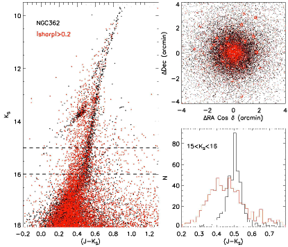
Figure 1.— Left: CMD of NGC 362 showing all stars which passed our photometric quality cuts (black) as well as those which failed the sharpness cut (red). The dashed horizontal lines indicate the magnitude range used to construct a color histogram of the lower red giant branch (lower right), illustrating the bias caused by stars with higher absolute values of the sharpness parameter. The spatial distribution of the two samples relative to the cluster center (upper right) illustrates the efficiency of the sharpness criterion to eliminate spurious detections.

In order to facilitate comparison and concatenation with existing GGC near-IR photometry (see Sect. 2.3) as well as direct comparison to multiple sets of evolutionary models (see Sect. 4.1), we have chosen to calibrate our instrumental catalogs to the 2MASS photometric system. Stars astrometrically matched to 2MASS were only used as photometric calibrators if they satisfied a more stringent set of criteria: They must be matched to a 2MASS point source to within the astrometric rms ($<$0.2$\arcsec$), isolated (lacking neighbors within 4 mag inside a 2.5$\arcsec$ radius, corresponding to a contaminating flux of $<$2.5%) and be bright enough to remain unaffected by crowding in 2MASS (see below). To calculate transformations from the instrumental magnitudes in our PSF catalogs to the 2MASS photometric system, we employed classical linear transformation equations of the form $m-M=a+b(J-K_{S})$, where $m$ and $M$ denote instrumental and standard magnitudes respectively. We solve for the coefficients $a$ and $b$ using least squares fitting, but employing weighting factors to downweight discrepant data points in lieu of a sigma clip (Mauro et al., 2013; Cohen et al., 2014), and we apply these same weighting factors to calculate the weighted root mean square deviation (wrms) of the residuals. A comparison between the results of our calibration procedure and the magnitudes reported in the 2MASS PSC are shown in Fig. 2, with the wrms given in each plot. The asymmetry seen at the faint end among stars positionally matched to 2MASS is due to the brighter completeness limit and lower spatial resolution of 2MASS, resulting in a systematic brightward deviation in 2MASS magnitudes. This effect serves as a cautionary note against calibrating to 2MASS in cases where only the faintest 2MASS stars are unsaturated, and for this reason we exclude faint 2MASS sources ($K_{S}\gtrsim$14 depending on stellar density) from use as photometric calibrators (see Fig. 2). Statistics regarding calibration uncertainties for each cluster, including the wrms values, photometric zero point uncertainties, and the number of stars from 2MASS used for photometric calibration, are summarized in Table 2. As our photometry saturates slightly below the tip of the cluster red giant branch in some cases, we have supplemented our catalogs with 2MASS photometry for bright stars which are absent due to saturation.

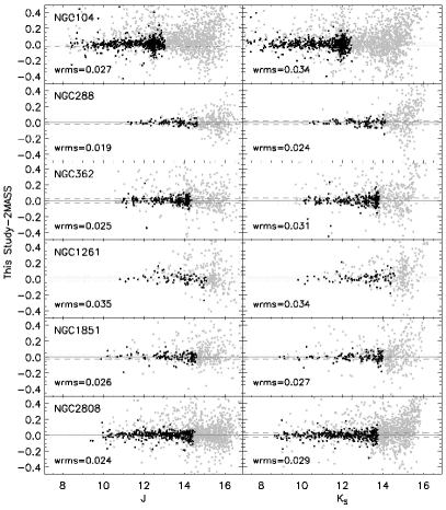
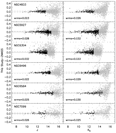
Figure 2.— A comparison of our calibrated photometry in the $J$ (left) and $K_{S}$ (right) filters with photometry from the 2MASS PSC. All matched stars are shown in grey, and 2MASS stars used for photometric calibration are overplotted in black. In each plot, the solid grey line represents equality while the dashed grey lines represent the weighted RMS deviation among the calibrators.

Table 2Photometric Calibration Uncertainties with Respect to 2MASS

Cluster	wrms		$\sigma(zpt)$		N
	$J$	$K_{S}$	$J$	$K_{S}$
NGC 104	0.027	0.034	0.005	0.006	647
NGC 288	0.019	0.024	0.013	0.017	89
NGC 362	0.025	0.031	0.007	0.010	222
NGC 1261	0.035	0.034	0.014	0.014	76
NGC 1851	0.026	0.027	0.010	0.011	118
NGC 2808	0.024	0.029	0.006	0.008	347
NGC 4833	0.023	0.026	0.009	0.010	164
NGC 5927	0.028	0.032	0.005	0.006	495
NGC 6304	0.032	0.033	0.010	0.011	360
NGC 6496	0.022	0.029	0.006	0.007	220
NGC 6584	0.025	0.030	0.007	0.009	135
NGC 7099	0.026	0.025	0.033	0.036	61

2.3. Comparison to Previous Photometry

Four of our target clusters have been observed by Valenti et al. (2004a, 2005), and near-IR photometry of 47 Tuc has been presented by Salaris et al. (2007), allowing a direct comparison of our 2MASS-calibrated $JK_{S}$ photometry to theirs. In all cases, we recover the majority of previously detected sources, and a cluster-by-cluster comparison of magnitude difference as a function of magnitude is shown in Fig. 3. There, we have computed the mean magnitude difference for each cluster in each filter using a weighted 2.5$\sigma$ clip in magnitude bins while excluding stars faintward of the observed luminosity function peak. Our calibrated photometry is in agreement with earlier studies in light of total calibration uncertainties, and although offsets of $>$0.05 mag are seen for NGC 288 in the $K_{S}$ band (and to a lesser extent NGC 7099 in $J$), the direct comparison to 2MASS in Fig. 2 gives no reason to be doubtful about the calibration of these clusters given our calibration uncertainties listed in Table 2 and the zeropoint uncertainty of $\pm$0.05 mag cited by Valenti et al. (2005).

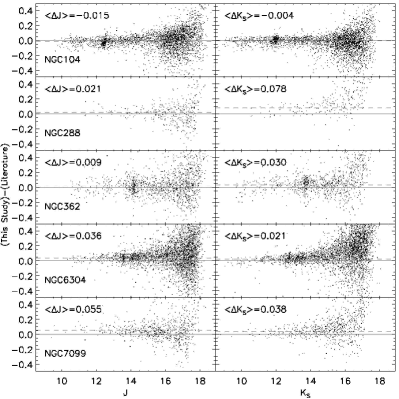
Figure 3.— Comparison of our 2MASS-calibrated $JK_{S}$ photometry with that of Salaris et al. (2007) for NGC 104 (top panel) and Valenti et al. (2004a) and Valenti et al. (2005) for the remainder of the clusters illustrated. The solid grey line represents equality, and the dotted grey line represents the mean offset, calculated using a 2.5$\sigma$ clip in bins of 1 mag and given in the upper left of each panel.

In addition, there is one cluster in our sample (NGC 1851) in common with the study of Brasseur et al. (2010). To compare their $(V-K_{S})$ fiducial sequence with our observations, we have matched our photometry to publicly available optical photometry from the archive of P. B. Stetson as well as the photometric catalog available from the ACS GGC Treasury Survey (Sarajedini et al., 2007). In the latter case, the offsets listed by Hempel et al. (2014) were applied to the Sirianni et al. (2005) transformed magnitudes to place them on the photometric system employed by Stetson. As the ACS catalogs are astrometrically calibrated to 2MASS (Anderson et al., 2008), a simple matching algorithm with an initial tolerance of 0.6$\arcsec$ and an iterative 5$\sigma$ clip functions well, and we recovered 99% of ISPI sources in the ACS field of view with an astrometric rms of 0.134$\arcsec$. The resulting matched CMD is shown in Fig. 4 with the optical-IR fiducial sequence of Brasseur et al. (2010) overplotted.

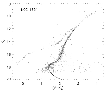
Figure 4.— Observed $K_{S},(V-K_{S})$ CMD of NGC 1851, obtained by matching our ISPI photometry with publicly available optical photometry (see text for details). The fiducial sequence of Brasseur et al. (2010) is overplotted as a black solid line.

3. Color-Magnitude Diagrams and Fiducial Sequences

3.1. Construction of Fiducial Sequences

To construct fiducial sequences representative of the RGB in each cluster, we fit a low-order ($n\leq$3) polynomial in the $(J-K_{S})$ vs. $K_{S}$ plane in a similar manner as previous studies (e.g. Ferraro et al., 1999, 2000; Cohen et al., 2014): First, a rough color-magnitude cut is made in the cluster CMD to select the region of the RGB. Next, the RGB is divided into bins of 0.5 mag, and the median color and magnitude (and their uncertainty) are calculated in each bin. A polynomial is then fit to these median points, iteratively rejecting stars more than 2$\sigma$ from the polynomial in each bin until convergence is indicated by the total number of stars remaining constant to within 2% since the previous iteration.

In Fig. 5 we present $J-K_{S},K_{S}$ CMDs of all of our target clusters, with the RGB fiducial sequences overplotted in red and median photometric errors in bins of 1 mag indicated along the right-hand side of each CMD. All varibles matched to our photometry from the most recent version of the Clement et al. (2010) catalog of variable stars in GGCs are overplotted as blue diamonds and excluded from further analyses.

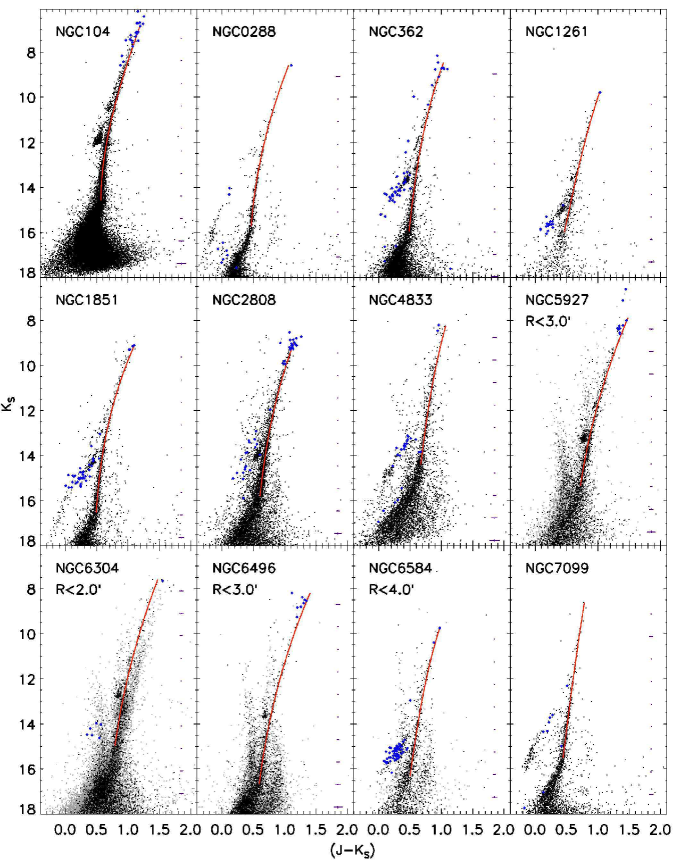
Figure 5.— CMDs of our target clusters, with fiducial sequences overplotted in red and known variables as blue diamonds. In cases where a radial cut was necessary to reduce field contamination, the location of the radial cut in arcmin from the cluster center is given, and stars outside this radius are plotted in grey rather than black. Median color and magnitude errors in bins of 1 mag are shown along the right side of each CMD.

Our photometric catalogs are available electronically, and their format is illustrated in Table 3.

Table 3NGC 104 Photometric Catalog

RA (J2000)	Dec (J2000)	$J$	$\sigma$$J$	$K_{S}$	$\sigma$$K_{S}$
6.283727	-72.069279	10.9506	0.0263	10.3440	0.0044
6.283700	-72.031622	14.2151	0.0155	13.7408	0.0075
6.283753	-72.133077	15.2417	0.0217	14.9558	0.0144
6.283345	-72.093668	16.7742	0.0621	16.5855	0.0298
6.283288	-72.071959	17.8108	0.0765	17.2019	0.0482
6.283036	-72.096528	17.0105	0.0611	16.9107	0.0429
6.282974	-72.112954	16.2559	0.0342	16.1854	0.0254
6.282944	-72.063674	11.2960	0.0234	10.6157	0.0042
6.282786	-72.060823	16.6431	0.0446	16.2261	0.0231
6.282719	-72.022186	17.9398	0.0723	17.4222	0.0490

Note. — The full photometric catalogs for all target clusters are available electronically; a portion is shown here to illustrate their form and content

3.2. The Absolute Magnitude Plane: Cluster Distance, Reddening and Metallicity

One of the primary goals of the present study is to use a self-consistent set of cluster distances, reddenings and metallicities to compare observed evolutionary sequences to models. Furthermore, with an eye towards heavily reddened stellar systems for which the use of optical photometry to measure cluster parameters is prohibitive, we also rederive empirical relations describing the RGB shape as a function of metallicity. To this end, we select distances and reddenings from D10 and $[Fe/H]$ (and uncertainties) from C09 . For consistency with D10 we employ the total to selective extinction ratios $R_{V}$ given by Sirianni et al. (2005) for a G2 star, and values of $A_{J}/E(B-V)$=0.899 and $A_{Ks}/E(B-V)$=0.366 from Casagrande & VandenBerg (2014). For the two GGCs excluded from D10 due to the presence of multiple stellar populations (NGC 1851, NGC 2808), we employ parameters obtained identically as for the remainder of the D10 sample (A. Dotter, private communication, also see Milone et al. 2014).

Our adopted values for the cluster distance moduli, reddening and metallicity are listed in Table 4. In light of cluster-to-cluster variations in $\alpha$-enhancement, we also calculate the global metallicity $[M/H]=[Fe/H]+Log(0.638f_{\alpha}+0.362)$ where $f_{\alpha}=10^{[\alpha/Fe]}$ (Salaris et al., 1993). Observed values of $[\alpha/Fe]$ from Carretta et al. (2010a) are listed in Table 4 where available, as well as the values we assume for our isochrone comparison (discussed below in Sect. 4.1). We also list the corresponding global metallicity $[M/H]$, including its uncertainty calculated following Nataf et al. (2013, see their eq. 7) and conservatively assuming $\sigma$$[\alpha/Fe]$=0.1. In Fig. 6, we display our fiducial sequences, shifted to the dereddened plane and color coded by $[Fe/H]$.

Figure 6.— Our fiducial sequences in the $M_{K},(J-K_{S})_{0}$ plane, color coded by $[Fe/H]$ value. Median photometric errors in magnitude bins are shown along the right-hand side.

Table 4Cluster Parameters

Cluster	RA (J2000)	Dec (J2000)	$(m-M)_{0}$	$E(B-V)$	$[Fe/H]$	$[\alpha/Fe]$	$[\alpha/Fe]$	$[M/H]$	$\Delta$$(V-I)$
						observed	assumed	assumed
NGC104	00:24:05.71	-72:04:52.7	13.26	0.023	-0.76$\pm$0.02	0.42	0.4$\pm$0.1	-0.47$\pm$0.08	0.153$\pm$0.003
NGC288	00:52:45.24	-26:34:57.4	14.83	0.013	-1.32$\pm$0.02	0.42	0.4$\pm$0.1	-1.03$\pm$0.08	1.022$\pm$0.025
NGC362	01:03:14.26	-70:50:55.6	14.76	0.023	-1.30$\pm$0.04	0.30	0.4$\pm$0.1	-1.01$\pm$0.09	0.195$\pm$0.003
NGC1261	03:12:16.21	-55:12:58.4	16.08	0.013	-1.27$\pm$0.08		0.4$\pm$0.1	-0.98$\pm$0.11	0.201$\pm$0.005
NGC1851	05:14:06.76	-40:02:47.6	15.42	0.020	-1.18$\pm$0.08	0.38	0.4$\pm$0.1	-0.89$\pm$0.11	0.234$\pm$0.011
NGC2808	09:12:03.10	-64:51:48.6	15.05	0.183	-1.18$\pm$0.04	0.33	0.4$\pm$0.1	-0.89$\pm$0.09	0.966$\pm$0.025
NGC4833	12:59:33.92	-70:52:35.4	14.19	0.359	-1.89$\pm$0.05		0.4$\pm$0.1	-1.60$\pm$0.10	0.900$\pm$0.029
NGC5927	15:28:00.69	-50:40:22.9	14.57	0.399	-0.29$\pm$0.07		0.2$\pm$0.1	-0.15$\pm$0.10	0.112$\pm$0.007
NGC6304	17:14:32.25	-29:27:43.3	13.99	0.481	-0.37$\pm$0.07		0.2$\pm$0.1	-0.23$\pm$0.10	0.105$\pm$0.004
NGC6496	17:59:03.68	-44:15:57.4	14.95	0.216	-0.46$\pm$0.07		0.2$\pm$0.1	-0.32$\pm$0.10	0.107$\pm$0.008
NGC6584	18:18:37.60	-52:12:56.8	15.71	0.079	-1.50$\pm$0.09		0.4$\pm$0.1	-1.21$\pm$0.12	0.408$\pm$0.062
NGC7099	21:40:22.12	-23:10:47.5	14.72	0.054	-2.33$\pm$0.02	0.37	0.4$\pm$0.1	-2.04$\pm$0.08	0.872$\pm$0.006

4. Models Versus Data on the Red Giant Branch

4.1. Adopted Models

Our observations are compared to the following sets of evolutionary models, all of which have been updated recently, including the capability to generate $\alpha$-enhanced isochrones:

1. Dartmouth Stellar Evolutionary Database (DSED; Dotter et al. 2008) isochrones with $[\alpha/Fe]$=0.4.

2. Victoria-Regina (VR; VandenBerg et al. 2014) isochrones with $[\alpha/Fe]$=0.4.

3. Bag of Stellar Tracks and Isochrones (BaSTI; Pietrinferni et al. 2006) canonical $\alpha$-enhanced isochrones.

4. Yale-Yonsei (YY; Yi, Kim & Demarque 2003; Demarque et al. 2004) isochrones with $[\alpha/Fe]$=0.4.

5. Princeton-Goddard-PUC (PGPUC; Valcarce, Catelan & Sweigart 2012) isochrones, with $[\alpha/Fe]$=0.3 (this is the highest degree of $\alpha$ enhancement available over GGC parameter space).

Any critical attempt to evaluate these models versus each other on equal footing is not truly an apples-to-apples comparison, as they all differ in various input assumptions (e.g. solar abundances, $\alpha$-enhanced chemical compositions, treatment of convection and atomic diffusion, color-$T_{eff}$ relations). However, a direct comparison between different near-IR isochrones has yet to be published, and comparisons between individual isochrones and high-quality data are scarce. Here we take advantage of our homogenous photometry of 12 GGCs covering a range of distance, reddening and metallicity to objectively explore how well existing isochrones fit observational data in the near-IR. That being said, in a few cases some modifications were made to the available default settings of various models in an attempt to maximize consistency. First, the near-IR colors and magnitudes output by the BaSTI and YY models are on the Johnson-Cousins-Glass photometric system (Bessell & Brett, 1988), so they were converted to the 2MASS photometric system using the relations of Carpenter (2001). Second, the VR and PGPUC models, rather than assuming a $\Delta$$Y/\Delta$$Z$ relation (or having one optionally available), give the user the ability to interpolate simultaneously in $Y$, $[\alpha/Fe]$ and $[Fe/H]$ (or $Z$). In these cases, we have chosen values of $Y$ in order to be consistent with D10 , increasing $Y$ slightly with $[Fe/H]$ to approximate a $\Delta$$Y/\Delta$$Z$=1.4 relation. In any case, minor model-to-model differences in $\Delta$$Y$ are inconsequential to our results since the location of the RGB in the near-IR is quite insensitive to He variations (see Sect. 4.4)

4.2. Cluster by Cluster Comparison

In Fig. 7, we compare the five sets of isochrones to observed ISPI photometry for eight of our target clusters with the highest quality photometry spanning the observed metallicity range. For increased clarity, we show two panels for each cluster, where the left panel directly overplots the isochrones on the observed photometry, and in the right panel we plot the color difference with respect to the observed fiducial sequence as a function of $M_{K}$. For this purpose, we conservatively approximate the uncertainty on the color of the fiducial sequence as the standard deviation of the color difference between the fiducial sequence and the observed RGB stars, calculated in moving bins of width 0.5 mag in $K_{S}$ using exclusively stars redward of the fiducial sequence to avoid contamination from the HB and AGB. The resulting color uncertainty as a function of magnitude is illustrated using dotted lines in the right-hand panel of Fig. 7 for each cluster. We employ models with $[\alpha/Fe]$=0.4 (except in the case of PGPUC as noted above), but for the three most metal-rich clusters (NGC5927, NGC6304, NGC6496, -0.46$\leq$$[Fe/H]\leq$0.29) we use models with $[\alpha/Fe]$=0.2. This choice is supported by both D10 and V13 , and is consistent with observed trends of $[\alpha/Fe]$ vs. $[Fe/H]$ as a function of Galactocentric radius and scale height (Hayden et al. 2015 and references therein) and the ”disklike” enrichment scenario employed in earlier studies (e.g. Ferraro et al., 1999; Ferraro, Valenti & Origlia, 2006).

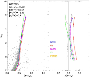
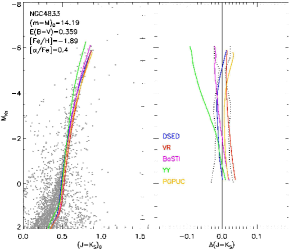
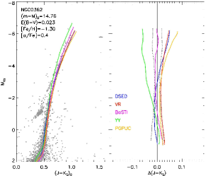
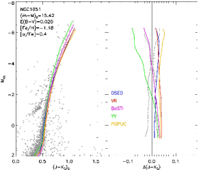
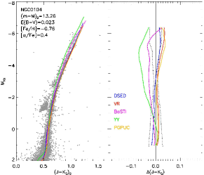
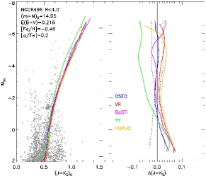
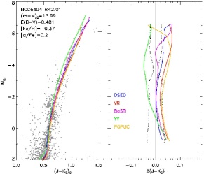
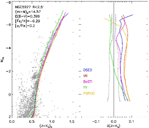
Figure 7.— Comparison between isochrones from five sets of evolutionary models and observed cluster photometry. For each cluster, the left panel illustrates the isochrones overplotted on the photometry, with median photometric errors given along the right hand side. The right panel illustrates the color difference between the models and the observed fiducial sequence as a function of absolute $K_{S}$ magnitude, where the vertical solid line represents equality and the dotted lines indicate the estimated color uncertainty of the fiducial sequence. Models are color coded as indicated in the right hand panel for each cluster.

Total agreement, either between models and data or among various sets of models, would be surprising due in part to the various model-to-model differences mentioned in Sect. 4.1. However, it appears that the DSED and VR models reasonably reproduce the observed morphology of the observed RGBs, although deviations in morphology from the fiducial sequences are still seen (as with all models investigated here). In addition, these deviations appear to become more drastic at low ($[Fe/H]\lesssim$-2) metallicities. While this result is fully consistent with the findings of Brasseur et al. (2010) using optical-IR colors, we caution that at least in our case, the formal statistical significance of these morphological deviations may not be high when photometric errors as well as calibration uncertainties are taken into account.

To quantify the color difference $\Delta(J-K_{S})$ between the observed RGB fiducial sequence and the five models shown in Fig. 7 for each cluster, we have calculated the mean and standard deviation (weighted using the observed errors shown as dotted lines in Fig. 7) of $\Delta(J-K_{S})$ in evenly spaced magnitude bins over the cluster RGBs ($M_{K}$$<$0). In this way, the mean quantifies the extent to which a model matches observed colors, averaged over the RGB, while standard deviation gauges the match in terms of CMD morphology. These statistics are given for all target clusters in Table 5, and are summarized across all clusters using the median and the median absolute deviation (MAD) in the last two rows. The results indicate that the DSED and VR models do the best job of reproducing the observed CMD morphology, although BaSTI and PGPUC do nearly as well in this sense, and the BaSTI models actually best agree with the observed fiducial colors in the mean.

Table 5Color Difference $\Delta(J-K_{S})$ Between Fiducial Sequences and Models

	DSED		VR		BaSTI		YY		PGPUC
Cluster	Mean	$\sigma$	Mean	$\sigma$	Mean	$\sigma$	Mean	$\sigma$	Mean	$\sigma$
NGC5927	-0.049	0.018	-0.071	0.009	-0.036	0.016	0.014	0.033	-0.053	0.028
NGC6304	-0.021	0.017	-0.040	0.017	-0.014	0.022	0.034	0.027	-0.044	0.014
NGC6496	0.002	0.016	-0.017	0.019	-0.004	0.026	0.039	0.044	-0.023	0.023
NGC0104	-0.001	0.011	-0.012	0.011	0.023	0.016	0.046	0.028	-0.012	0.012
NGC1851	-0.023	0.008	-0.031	0.007	-0.003	0.020	0.031	0.040	-0.035	0.006
NGC2808	-0.008	0.019	-0.014	0.008	0.020	0.012	0.059	0.033	-0.026	0.021
NGC1261	-0.017	0.017	-0.032	0.016	-0.007	0.019	0.026	0.035	-0.033	0.020
NGC0362	-0.005	0.020	-0.020	0.009	0.004	0.010	0.037	0.026	-0.021	0.020
NGC0288	-0.012	0.008	-0.033	0.021	-0.008	0.033	0.016	0.054	-0.032	0.012
NGC6584	-0.008	0.018	-0.028	0.013	-0.000	0.018	0.038	0.036	-0.029	0.019
NGC4833	0.006	0.007	-0.016	0.008	0.013	0.013	0.057	0.037	-0.015	0.009
NGC7099	-0.016	0.011	-0.046	0.012	-0.022	0.014	0.008	0.030
Median	-0.008	0.017	-0.028	0.012	-0.003	0.018	0.037	0.035	-0.029	0.019
MAD	0.009	0.004	0.012	0.003	0.011	0.005	0.011	0.005	0.006	0.005

We discuss practical ramifications of this result further in Sect. 6.2, and now explore the effects of variations on $[\alpha/Fe]$ and helium predicted by the models, in order to gain insight into the role of uncertainties in these quantities.

4.3. Model Predictions: $[\alpha/Fe]$ Variations

The difference between scaled solar isochrones versus those which are $\alpha$-enhanced (at fixed $Y$ and $[Fe/H]$) are illustrated in Fig. 8. There, the $(J-K_{S})_{0}$ color difference between isochrones with $[\alpha/Fe]$=0.4 and 0 are plotted in the sense ($\alpha$-enhanced$-$scaled solar), for a regular grid of $[Fe/H]$ values spanning the values of the target clusters. To illustrate the influence of $\alpha$-enhancement in the near-IR on the main sequence, we extend these plots faintward beyond the lower main sequence knee (MSK). A couple of features are evident: First, all of the models except for BaSTI give schematically similar predictions regarding the effect of $\alpha$-enhancement on the upper RGB at low to intermediate (-2$\leq$$[Fe/H]\leq$-1) metallicities. Specifically, an enhancement of $[\alpha/Fe]$=0.4 dex shifts the upper RGB redward by 0.05 mag or more in $(J-K_{S})$ color (depending on the model and the $[Fe/H]$ value), larger than seen anywhere else in the CMD with the exception of the lower ($M_{K}$$>$5) main sequence. Meanwhile, the lower RGB (0$\lesssim$$M_{K}$$\lesssim$2) remains less affected save for a slight $\sim$0.02 mag redward shift. However, approaching solar metallicity, the model predictions diverge somewhat, with some (DSED, VR) predicting a negligible effect on the RGB tip but maintaining a redward shift over the remainder of the RGB.

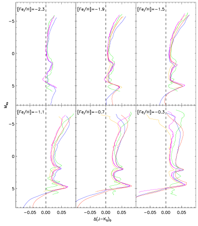
Figure 8.— The color difference between an $\alpha$-enhanced isochrone and a scaled solar isochrone for each model as a function of absolute $K_{S}$ magnitude. The difference is plotted in the sense ($\alpha$-enhanced$-$scaled solar), and color coded by model as in previous figures.

4.4. Model Predictions: Helium Enhancement

Much effort has recently been devoted to the issue of a spread or enhancement in helium among GGC (sub-) populations, as there are important implications for GGC formation. Therefore we briefly examine to what extent a change in helium abundance influences near-IR GGC CMDs. The result of an increase of $\Delta$$Y$=0.04 (at fixed $[\alpha/Fe]$=0.4) is shown in Fig. 9, again at a range of $[Fe/H]$ values. Only the VR models are shown, although the results are nearly identical for other models, which is that near-IR colors on the RGB are minimally affected ($\Delta$$(J-K_{S})$$<$0.01 at fixed $M_{K}$), with essentially no consequences for the RGB morphology. As it has been demonstrated that the MSTO and MSK can be used as age indicators in the near-IR (Bono et al., 2010), we point out that while helium enhancement shifts the MSTO and the RGB very slightly blueward in color, these shifts are equivalent to $<$0.01 mag. Similarly, the magnitude of the MSTO and MSK are shifted faintward by nearly equal amounts ($<$0.1 mag, see Fig. 10). For this reason, a modest helium spread or enhancement in the near-IR is of little consequence for age determinations employing relative CMD indices (e.g. V13, ).

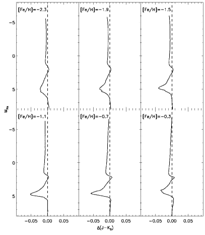
Figure 9.— The $J-K_{S}$ color difference predicted for a helium enhancement of $\Delta$$Y$=0.04 from $[\alpha/Fe]$=0.4 VR models at a range of $[Fe/H]$. The difference is plotted in the sense (helium enhanced-helium normal).

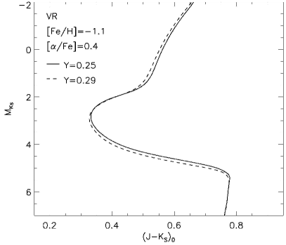
Figure 10.— The effect of helium enhancement in the near-IR, using VR isochrones with a fixed $[\alpha/Fe]$=0.4 and $[Fe/H]$=-1.1, shown for $Y$=0.25 (solid line) and $Y$=0.29 (dotted line).

4.5. Photometric Indices

Previous studies (Frogel, Cohen & Persson, 1983; Cohen & Sleeper, 1995; Ferraro et al., 2000; Valenti et al., 2004a), cognizant of the fact that the RGB becomes increasingly sensitive to metallicity at higher luminosities, developed a set of photometric indices to characterize the upper RGB as a function of metallicity in the near-IR. These indices include (dereddened) color at fixed (absolute) magnitude, specifically $(J-K_{S})_{0}$ at $M_{K}$=(-3,-4,-5,-5.5), as well as absolute magnitude $M_{K}$ at $(J-K_{s})_{0}$=0.7. As Ferraro et al. (2000) point out, the use of indices constructed purely using IR filters has the advantage of decreased sensitivity to uncertainties in both distance, due to the near-vertical slope of the RGB (e.g. Valenti et al., 2004a), and reddening ($E(J-K_{S})$=0.533$E(B-V)$; Casagrande & VandenBerg 2014). These indices can be employed to measure cluster distances, reddenings and metallicities (e.g. Ferraro, Valenti & Origlia, 2006), and also provide another approach to quantifying discrepancies between isochrones and observed fiducial sequences. Therefore, in Fig. 11 we present new relations between these photometric indices as function of both cluster $[Fe/H]$ and global metallicity $[M/H]$ as well as a comparison with the five sets of evolutionary models listed in Sect. 4.1. The uncertainties in dereddened color are calculated as described in Sect. 4.2, and our linear fits are performed taking uncertainties in both axes into account. The resulting equations and the rms deviation of the residuals is given in each panel of Fig. 11, as well as inverted versions of these equations (with $[Fe/H]$ or $[M/H]$ as the dependent variable) and the corresponding x-axis rms. The relations of Valenti et al. (2004a), transformed to the metallicity scale of C09 , are overplotted as dotted lines for comparison. It appears that a linear fit is a reasonable representation of $(J-K_{S})_{0}$ color as a function of $[Fe/H]$ and $[M/H]$, with a slope that increases with luminosity, in general accord with previous results (Ferraro et al., 2000; Valenti et al., 2004a).

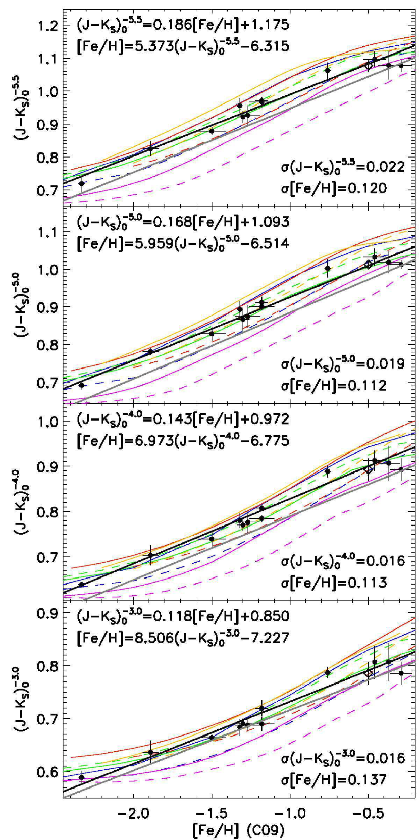
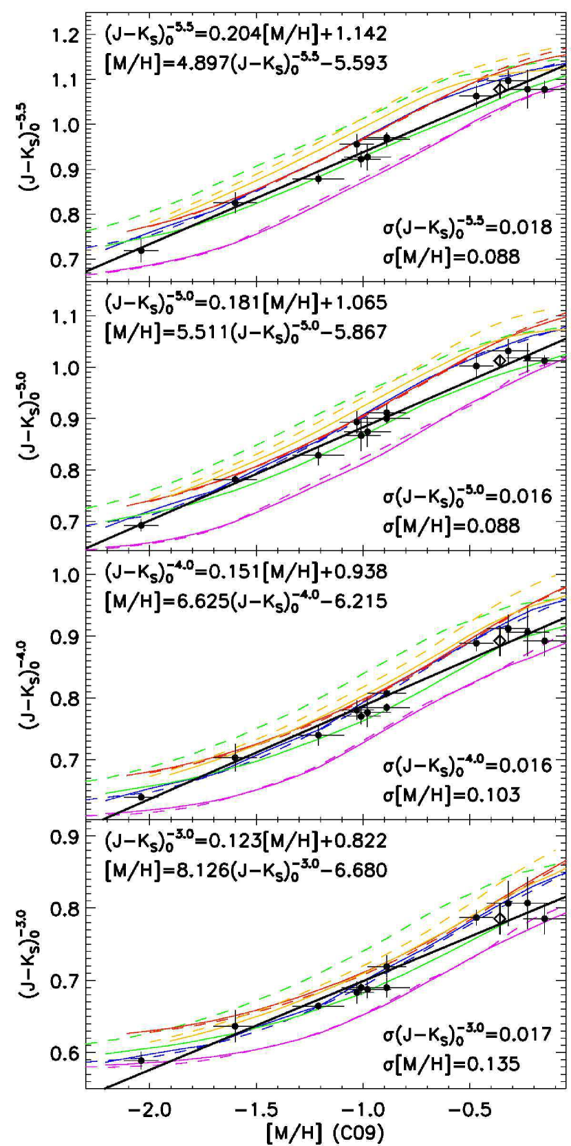
Figure 11.— Indices of dereddened $(J-K_{S})_{0}$ color at fixed absolute magnitude $M_{K}$=-5.5, -5, -4 and -3 (top to bottom) as a function of $[Fe/H]$ (left) and $[M/H]$ (right). Vertical error bars represent measurement uncertainties only and do not include uncertainties in cluster distance and reddening (see text for details). Predictions of evolutionary models are overplotted using the same colors as in Fig. 7, where models with $[\alpha/Fe]$=0.4 are shown as solid lines and models with $[\alpha/Fe]$=0 are shown as dashed lines. A linear fit is shown as a black solid line, with the coefficients and the rms deviation given in the upper left of each panel. The relations of Valenti et al. (2004a), converted to the C09 metallicity scale, are overplotted as grey lines in the left panels. The open diamond represents the value for NGC 5927 assuming a metallicity of $[Fe/H]$=-0.5 (see Sect. 6.2).

Dereddened color at fixed absolute magnitude can also be used to characterize the RGB, as these indices sample a luminosity range which is dependent on metallicity (this is apparent, for example, in Fig. 6). In Fig. 12 we present linear fits of $M_{K}$ at fixed $(J-K_{S})_{0}$=0.7, again as a function of $[Fe/H]$ and the global metallcity $[M/H]$. In this case, the observational magnitude uncertainty has been calculated by multiplying the observed color uncertainty by the slope of the fiducial sequence at the corresponding magnitude. The resulting fits are shown in Fig. 12, again with $[\alpha/Fe]$=0.4 and 0.0 models and the fits of Valenti et al. (2004a) shown for comparison.

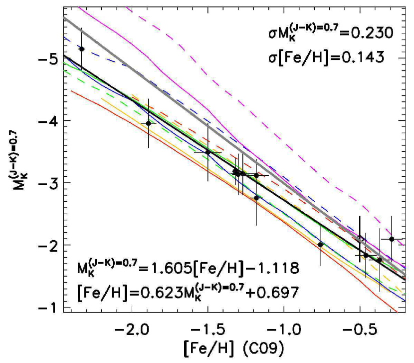
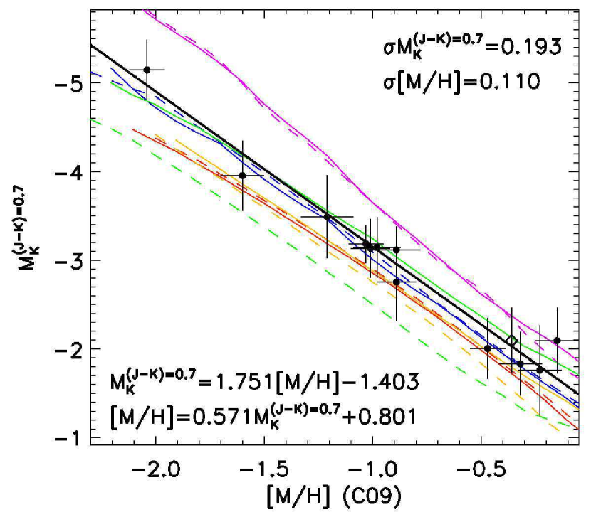
Figure 12.— Absolute magnitude $M_{K}$ at fixed color $(J-K_{S})_{0}$=0.7 as a function of $[Fe/H]$ (left) and $[M/H]$ (right). Symbols are as in Fig. 11.

Indices of color at fixed magnitude, unlike magnitude at fixed color, are extremely sensitive to cluster reddening values, as even the most metal-rich GGCs have RGB slopes of $|\delta(J-K_{S})/\delta$$K_{S}|$$<$0.12 (Valenti et al., 2004a, 2010; Chun et al., 2010). This is an advantage when using color at fixed magnitude to describe the RGB, since a moderate uncertainty in $[Fe/H]$ or $[M/H]$ does not have drastic consequences for the determination of distance and reddening. For example, the slope of the relation in the upper left panel of Fig. 11 implies that $\sigma[M/H]$=0.3 dex translates to $\sigma$$A_{K}\sim$0.03. On the other hand, an uncertainty of $\sigma$$E(J-K_{S})\sim$0.02, or $\sigma$$E(B-V)\sim$0.04, could account for a scatter of $\sim$0.2 mag in the relations presented in Fig. 12, although in the present case observational uncertainties appear to dominate. Interestingly, the quality of the linear fits in Figs. 11 and 12 improve at higher luminosities when the global metallicity $[M/H]$ rather than $[Fe/H]$ is employed, demonstrating that the upper RGB in the near-IR is quantifiably affected by cluster $[\alpha/Fe]$ consistent with the model predictions in Sect. 4.3. Our linear fits generally compare well to those of Valenti et al. (2004a) given their uncertainties, and we find nearly identical slopes in the case of color at fixed magnitude (Fig. 11). While zero point offsets are seen, these offsets are not large compared to the residuals of the Valenti et al. (2004a) fits, and can likely be explained by current uncertainties in cluster distances and reddenings (discussed later in Sect. 6.1).

5. Horizontal Branch and Red Giant Branch Bump Magnitudes

5.1. Near-IR Horizontal Branch Magnitude

In order to measure the magnitudes of our target cluster HBs, we first divide our sample into ”red HB” (RHB) and ”blue HB” (BHB) clusters. This division is made using the $\Delta$$(V-I)$ index of D10 (given in Table 4), which is less vulnerable to saturation at its extremes than $(B-R)/(B+V+R)$ (e.g. fig. 2 of D10 ). We consider the seven clusters with $\delta$$(V-I)$$<$0.3 as RHB clusters, and the remainder as BHB clusters, for the straightforward reason that all of the RHB clusters have HB LFs which show reliably detected peaks in magnitude whereas the BHB clusters have HBs which do not create a significant peak in their luminosity functions. The HB morphology of the BHB clusters is therefore not easily characterized using magnitude alone due to the diagonality of BHBs in near-IR CMDs (for this reason, we have included NGC 6584 among the BHB clusters despite its value of $\delta$$(V-I)$=0.408) so we present HB magnitudes for only the RHB clusters.

The location of the HB in $J$ and $K_{S}$ magnitude is quantified by constructing a luminosity function (LF) from the observed cluster CMD, and then identifying the location of the peak in this LF. To mitigate the effects of binning on the final LF, we construct a multi-bin histogram that is the average of 10 individual LFs in which the bin starting points were shifted by 0.1 times the chosen binsize and these 10 LFs are averaged. For clusters which have at least a portion of their comparison fields outside of their Harris (1996, 2011 revision) tidal radii (including the most heavily contaminated GGCs NGC5927, NGC6304 and NGC6496) this procedure was repeated for the comparison field CMD, before scaling the field LF by the relative cluster to field area and subtracting it from the cluster LF. An example is illustrated in Fig. 13. The uncertainty in the location of the LF peak is quantified using a simple Monte Carlo procedure wherein for each of 1000 iterations, the magnitude of each star in each filter is offset by a random amount drawn from a Gaussian distribution with a standard deviation equal to the photometric error. The construction of the LFs is then repeated, including the generation of the multi-bin histograms, and the location of the peak magnitude in each iteration reported. The uncertainty in the magnitude of the LF peak is then the standard deviation of the reported LF peak locations over the 1000 Monte Carlo iterations. Typically, this uncertainty was smaller than a resolution element of the LF (0.01-0.03 mag), so to be conservative, the two values were added in quadrature to obtain the final HB magnitude uncertainty, given in Table 6.

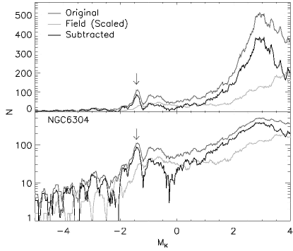
Figure 13.— An example luminosity function for the case of NGC 6304, the most heavily contaminated cluster in our sample, shown on a linear (top) and logarithmic (bottom) scale. After constructing a multi-bin LF from the cluster CMD (dark grey line), an LF is constructed for a comparison field, scaled by the ratio of cluster to field area (light grey line) and subtracted to obtain the decontaminated cluster LF (black line). The observed LF peak is indicated by a vertical arrow in both panels.

We plot the reported HB magnitudes as a function of $[M/H]$ in Fig. 14, color coded by the cluster age from D10 . In addition, we overplot the predictions of Salaris & Girardi (2002) as dashed lines after converting their $M_{K}$ values to the 2MASS system (Carpenter, 2001), since this remains the only study directly predicting HB magnitudes in the near-IR as a function of cluster age and metallicity which extends to the (low metallicity, high age) parameter space occupied by GGCs. At the metallicity of 47 Tuc and higher, our results are in agreement with Salaris & Girardi (2002) given uncertainties on absolute age ($\geq$0.5 Gyr from measurement errors alone; D10 ), but at lower metallicities, the models overestimate the $K$-band luminosity of the HB by as much as 0.1 mag in the case of NGC 1851. This issue should clearly be revisited with a larger sample of GGCs, and inter- and intra-cluster abundance variations not included in the Salaris & Girardi (2002) models could possibly account for this discrepancy, but perhaps a more likely possibility is simply the remaining uncertainty in the GGC distance and age scales (this is discussed further in Sect. 6.1). However, a dependence of $M_{K}(HB)$ on metallicity for GGCs has been observed at least since the study of Grocholski & Sarajedini (2002), and the observed HB magnitudes are not the culprit: The median HB magnitudes of Grocholski & Sarajedini (2002), measured directly from 2MASS, differ from ours by $<$0.04 mag (after accounting for the offset of 0.044 mag between photometric systems; Carpenter 2001) for both GGCs included in their study (47 Tuc and NGC 362).

We note that our comparison to Grocholski & Sarajedini (2002) and Salaris & Girardi (2002) is not strictly homogenous, as the former use the median of a CMD-selected region to characterize the HB magnitude and the latter give a mean HB magnitude. However, we found that employing any of these alternate techniques yielded HB magnitudes which differed from the LF peak by $\lesssim$0.02 mag in the mean, so that in this case, the choice of methodology for quantifying the HB peak does not significantly impact our conclusions, although radial population gradients which vary with HB color (for example due to light element abundance variations cf. Gratton et al. 2010) could play a role.

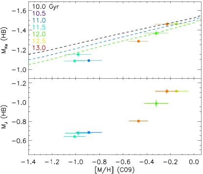
Figure 14.— Horizontal branch absolute magnitude in the $K_{S}$ (top) and $J$ (bottom) filters versus cluster $[M/H]$ for RHB clusters. In the upper panel, the predictions of Salaris & Girardi (2002) are overplotted as dashed lines after transformation to the 2MASS photometric system (Carpenter, 2001), and cluster and model predictions are both color coded by age as indicated in the top left of the upper panel.

5.2. The Red Giant Branch Bump (RGBB)

The magnitude of the RGBB is measured using a procedure similar to that of Nataf et al. (2013). Specifically, the RGB LF of a cluster is built using stars selected from the CMD (e.g.  see Fig. 15), and multibin histograms are used to construct the LF as described in the previous section. Again, the field LF (constructed from an identical CMD region as the cluster LF) is subtracted where feasible. Next, an exponential plus Gaussian function is fit to the resulting cluster RGB LF (e.g. Nataf et al., 2013) to measure the location of the RGBB, and an example of this procedure is shown in Fig. 16. Similar to Sect. 5.1, Monte Carlo simulations (over 1000 iterations) are used to quantify the uncertainty on the RGBB magnitude in each bandpass, wherein for each iteration, each star is offset by a Gaussian deviate of its photometric error, the multibin LF is reconstructed, an exponential plus Gaussian function is refit, and the resulting best fit location of the Gaussian peak is reported. The errors reported here were then calculated as the quadrature sum of the fit uncertainty to the observed RGBB plus the standard deviation of the best fit RGBB magnitude across the Monte Carlo iterations.

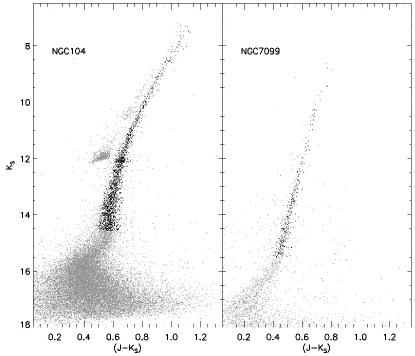
Figure 15.— Examples of the selection of RGB stars for the construction of the RGB LF, shown for the cases of NGC 104 (47 Tuc; left) and NGC 7099 (M30; right). All cluster sources are shown in grey, and stars used to construct RGB LFs are shown in black for each cluster.

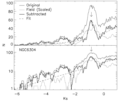
Figure 16.— Example $K_{S}$-band RGB LF for NGC 6304, shown on a linear (top) and logarithmic (bottom) scale. Symbols are as in Fig. 13 and the exponential plus Gaussian fit used to quantify the RGBB magnitude (indicated by the vertical arrow) is shown as a dotted line.

The resulting bump magnitudes and their uncertainties are listed in Table 6, and the RGBB absolute magnitude in each filter, $M_{J}(RGBB)$ and $M_{K}(RGBB)$ are shown in Fig. 17 as a function of both $[Fe/H]$ and $[M/H]$. Similarly to Valenti et al. (2004b), we were unable to detect the RGBB in NGC 7099. However, by matching our near-IR data to the optical photometry by Sarajedini et al. (2007) we were able to combine the $V$-band magnitude of the RGBB from Nataf et al. (2013) with its $(V-K_{S})$ color to calculate the $K_{S}$ magnitude of the RGBB, shown in Fig. 17. Next, we combined our sample with clusters from Cho & Lee (2002) and Valenti et al. (2004b) which have high-quality distances, reddenings and spectroscopic metallicities (C09, ; Carretta et al., 2010a; D10, ), and performed a quadratic fit for direct comparison with previous results. The relation of Valenti et al. (2004b) converted to the C09 scale appears to deviate from ours at high (near solar) metallicity, and we urge further multi-object spectroscopic studies of the most metal-rich GGCs to confirm this result. However, transforming the Valenti et al. (2004b) relation on the metallicity scale of Carretta & Gratton (1997) to the scale of C09 comes with the caveat that the transformation between these scales is in fact poorly defined at high metallicities, as none of the 13 clusters employed to derive the linear transformation between scales are more metal rich than 47 Tuc (see fig. 8 of C09 ).

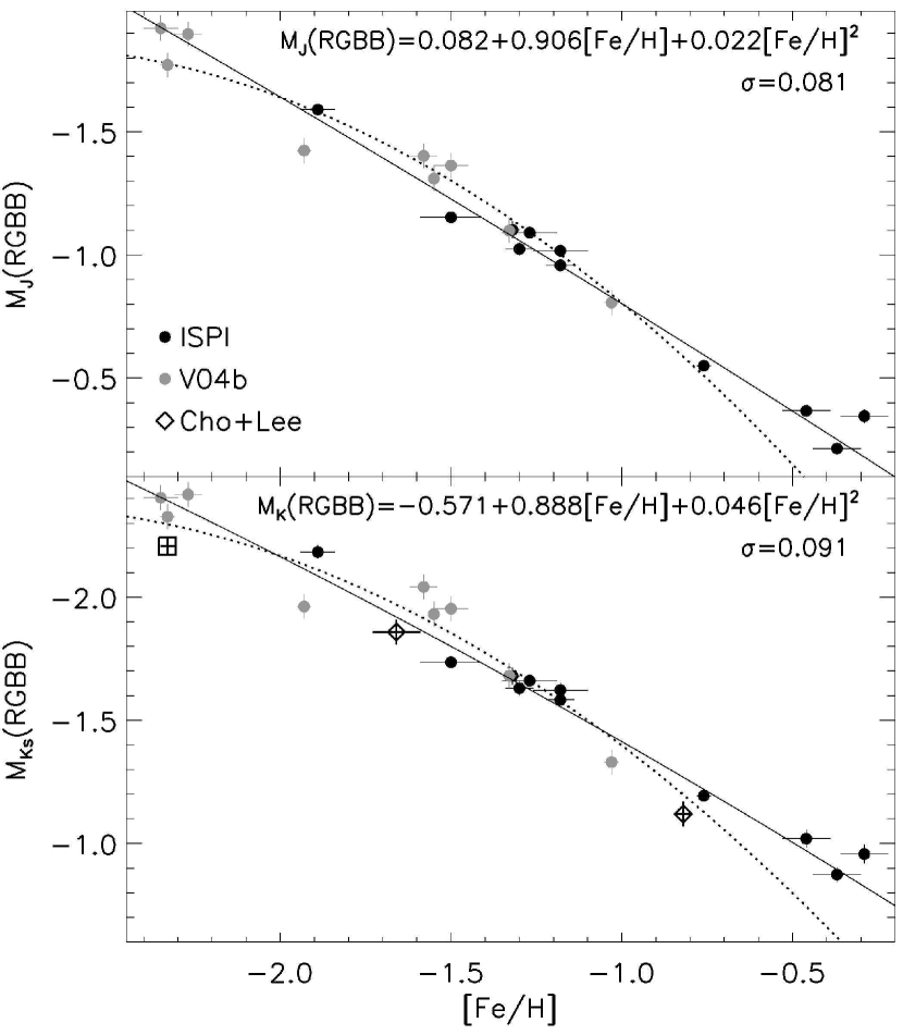
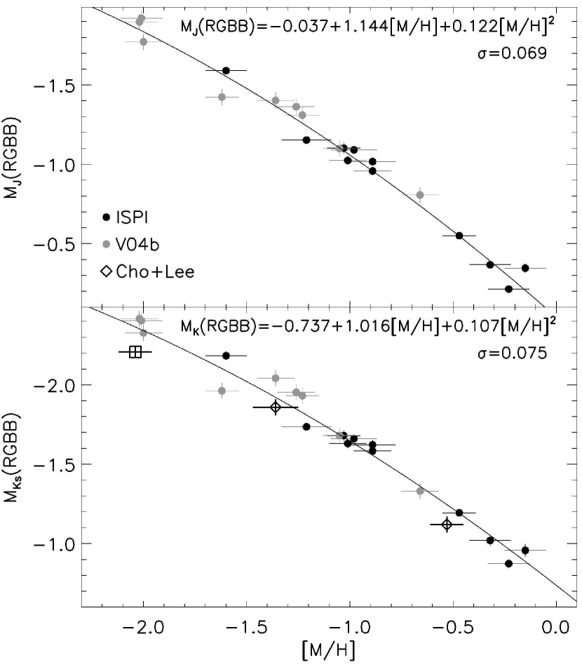
Figure 17.— Red giant branch bump absolute magnitude in the $J$ (upper panels) and $K_{S}$ (lower panels) filters versus cluster metallicity, in terms of $[Fe/H]$ (left) and $[M/H]$ (right). Filled black circles represent values for ISPI target clusters, grey circles are from Valenti et al. (2004b), and black open diamonds are from Cho & Lee (2002). The black square represents the RGBB location of NGC7099 predicted from optical-infrared photometry (see text) and has not been included in the fits. The solid line is a quadratic fit (with the resulting coefficients given in the upper right of each panel), and the dotted line represents the relation of Valenti et al. (2004b), transformed to the C09 $[Fe/H]$ scale.

Table 6Red Giant Branch Bump and Horizontal Branch Magnitudes

Cluster	$M(RGBB)$		$M(HB)$
	$J$	$K_{S}$	$J$	$K_{S}$
NGC0104	12.728$\pm$0.010	12.072$\pm$0.009	12.492$\pm$0.013	11.979$\pm$0.013
NGC0288	13.736$\pm$0.035	13.150$\pm$0.034
NGC0362	13.754$\pm$0.026	13.136$\pm$0.029	14.155$\pm$0.011	13.680$\pm$0.011
NGC1261	14.997$\pm$0.009	14.420$\pm$0.009	15.418$\pm$0.022	14.928$\pm$0.026
NGC1851	14.424$\pm$0.025	13.808$\pm$0.028	14.775$\pm$0.012	14.340$\pm$0.011
NGC2808	14.253$\pm$0.013	13.530$\pm$0.012
NGC4833	12.917$\pm$0.014	12.133$\pm$0.028
NGC5927	14.585$\pm$0.027	13.760$\pm$0.038	14.036$\pm$0.013	13.254$\pm$0.011
NGC6304	14.211$\pm$0.017	13.295$\pm$0.029	13.577$\pm$0.022	12.709$\pm$0.024
NGC6496	14.783$\pm$0.024	14.015$\pm$0.035	14.288$\pm$0.036	13.666$\pm$0.030
NGC6584	14.624$\pm$0.011	13.999$\pm$0.010

6. Discussion

6.1. Uncertainties in Cluster Parameters

To maximize homogeneity we consistently use the latest compilation of GGC distances and reddenings from D10 , which are based on fits of DSED isochrones to deep optical photometry from Sarajedini et al. (2007). While a detailed discussion of the GGC distance scale is beyond the scope of this investigation, recent studies estimate current uncertainties at the level of $\sim$0.10-0.15 mag (V13, ; VandenBerg, 2013, and references therein), consistent with a direct comparison between the distances reported by D10 versus those obtained via subdwarf fitting to the GGC main sequences (Cohen & Sarajedini, 2012).

In the current context, we revisit the comparison from Cohen et al. (2014, see their fig. 12) between the results of D10 and V13 with regard to GGC distances, reddenings, and metallicities. This comparison is especially useful since both investigations employed identical photometric catalogs from Sarajedini et al. (2007), but different strategies to obtain cluster parameters. On the one hand, D10 optimized their isochrone fits for the unevolved main sequence and the lower RGB, using values from the Harris (1996) catalog as initial guesses and allowing slight variations to $[Fe/H]$, $(m-M)_{F814W}$ and $E(F606W-F814W)$ when necessary. On the other hand, V13 fit model ZAHBs to the observed lower envelope of cluster HBs to measure ages, restricting these models to the C09 $[Fe/H]$ values and a two part linear $[\alpha/Fe]$-$[Fe/H]$ relation.

In Fig. 18, we present a comparison between the $(m-M)_{0}$, $E(B-V)$, $[Fe/H]$ and age values employed by D10 and V13 . The distance discrepancy between the two studies is generally within the aforementioned uncertainties ($\lesssim$0.1 mag), and the reddening values are in particularly excellent agreement. We also investigate the relevance of the difference in metallicities between the spectroscopic values reported by C09 which we employ and the values used by D10 for their isochrone fitting. The two sets of values are generally in good agreement (see Fig. 18), and D10 discuss the role of uncertainties in $[Fe/H]$ in some detail. However, in two cases the metallicities employed by D10 for their isochrone fits differ significantly from C09 : First, for NGC 5927 ($[Fe/H]$(C09, )=-0.29$\pm$0.07; $[Fe/H]$(D10, )=-0.5), the most metal rich cluster in our sample, distance and reddening are unlikely to play a role as both $E(J-K_{S})$ and $(m-M)_{K}$ agree to $\leq$0.01 mag between D10 and V13 . Furthermore, transformations of earlier $[Fe/H]$ measurements for this cluster to the C09 scale rest fairly heavily on the value obtained by Carretta et al. (2001) for NGC 6528 (see figs. A.1 and A.2 of C09 ), while subsequent observations of NGC 6528 imply lower values and a substantial ($\sim$0.2 dex) spread in $[Fe/H]$ (e.g. Zoccali et al., 2004; Sobeck et al., 2006; Mauro et al., 2014). The other significant discrepancy in cluster metallicity between C09 and D10 is the case of NGC 4833 ($[Fe/H]$(C09, )=-1.89$\pm$0.05; $[Fe/H]$(D10, )=-2.4). Recent spectroscopic evidence clarifies the situation to some degree: On one hand, Carretta et al. (2014) report $[Fe/H]$=-2.015$\pm$0.09 dex from UVES spectra on their C09 scale, but Roederer & Thompson (2015) find $[Fe/H]$=-2.25$\pm$0.02 from Fe I lines and $[Fe/H]$=-2.19$\pm$0.013 from Fe II lines, although they show that the use of different model atmosphere grids and line analysis codes can fully account for the discrepancy between their results and the Carretta et al. (2014) value. Fortunately, the aforementioned issues are of little consequence for the results of Figs. 11, 12 and 17. In fact, if we use values of $(m-M)_{0}$ and $E(B-V)$ from V13 and/or $[Fe/H]$ values from the D10 isochrone fits (rather than the spectroscopic values of C09 ), the fits in Figs. 11, 12 and 17 are unaffected to within their rms deviations. Alternatively, we could have simply excluded NGC 4833 and/or NGC 5927 from our fits, but this also turns out not to impact the fits beyond their uncertainties.

Our result from Sect. 5.1 that the Salaris & Girardi (2002) models overestimate the HB luminosity for metal-intermediate ($[M/H]\lesssim$-0.8) RHB clusters is also robust to the choice of distances, reddenings, and ages from V13 rather than D10 . This is due at least partially to the fact that although the absolute ages of V13 are generally younger than those of D10 , the relative ages of our target clusters are unchanged within their quoted uncertainties regardless of which set of absolute ages one assumes (see Fig. 18, bottom panel). In fact, the use of distances, reddenings and ages from V13 rather than D10 actually increases the discrepancy between observed and predicted $M_{K}$ at lower metallicities: Taking reported age and metallicity uncertainties into account, the shift required to bring observed $M_{K}(HB)$ values into accord with the Salaris & Girardi (2002) models at the 1$\sigma$ level is $\Delta$$M_{K}(HB)$=-0.15 and -0.17 mag for NGC 362 and NGC 1851 respectively, compared to $\Delta$$M_{K}(HB)$=-0.05 and -0.10 mag respectively (see Fig. 14) using the D10 distance, reddening and age. However, we recall that the distances and reddenings given by V13 were determined by assuming the lower envelope of the observed HB as the ZAHB (at the high-mass end). This procedure comes with the risk that any dependence on metallicity of the magnitude difference between the model ZAHB and the observed lower envelope of the HB (as discussed extensively, for example, by Ferraro et al. 1999 and Catelan 2009) could systematically bias our results. For this reason, the distances and reddenings of D10 appear a somewhat more objective set of values with which to investigate a relation between HB absolute magnitude and metallicity, in the sense that their isochrone fits, optimized for the cluster main sequences and lower RGB, give distances and reddenings perhaps more “independently” of the HB. We also caution that the interplay between HB morphology and other cluster parameters, including age, metallicity, light element abundances, and helium abundance, appears extremely complex and is under active investigation (e.g. Catelan, 2009; Gratton et al., 2010; D10, ; Milone et al., 2014). As our data are affected by central incompleteness, we cannot exclude the possibility that radial gradients in HB (sub-) populations (e.g. Nataf et al., 2011; Krogsrud et al., 2013; Vanderbeke et al., 2015) play a role. Therefore, a more detailed comparison between observed and synthetic HBs is a topic better tackled using high spatial resolution imaging of cluster cores.

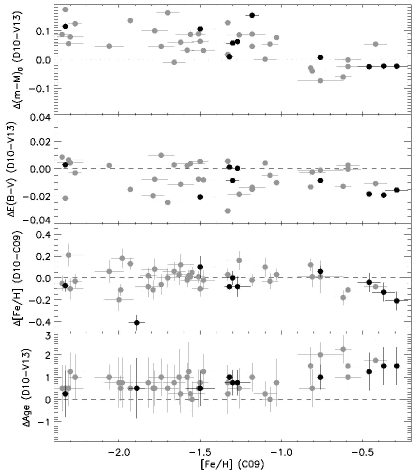
Figure 18.— Comparison of difference in $(m-M)_{0}$, $E(B-V)$, $[Fe/H]$ and cluster age in Gyr (top to bottom respectively) between D10 and V13 as a function of $[Fe/H]$ from C09 . The dashed line in each plot represents equality, and our target clusters are overplotted in black.

Differences in cluster distances and reddenings may also be responsible for minor differences between our fits and those of Valenti et al. (2004a, b) in Figs. 11, 12 and 17. In Fig. 19, we plot the difference in $(m-M)_{0}$ and $E(B-V)$ between D10 and Ferraro et al. (1999), the latter of which was employed by Valenti et al. (2004a, b) to calibrate their near-IR relations. Again, our target clusters are shown as filled black circles, and we have overplotted the Valenti et al. (2004a, b) calibrating clusters common to D10 with diamonds. Unlike the comparison between D10 and V13 , variations in cluster distance and reddening range up to $>$0.1 mag in $E(B-V)$ and $>$0.2 mag in $(m-M)_{0}$ (albeit in the opposite sense: clusters with longer distances have smaller reddening values). The lower reddenings of Ferraro et al. (1999) are a likely contributor to the blueward offset of the Valenti et al. (2004a) relations in Fig. 11 (recall that near-IR color at fixed magnitude is more sensitive to reddening than distance), as well as the brightward offset of their relation in Fig. 12. However, it is possible to explain the offset between our relations and those of Valenti et al. (2004a, b) without invoking differences in calibrating cluster distances and reddenings given the calibration uncertainties, measurement uncertainties and fit quality obtained here and by Valenti et al. (2004a, b).

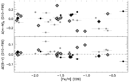
Figure 19.— Comparison of difference in $(m-M)_{0}$ (top) and $E(B-V)$ (bottom) between Ferraro et al. (1999) and D10 as a function of $[Fe/H]$ from C09 . Clusters present in both Ferraro et al. (1999) and D10 are shown as grey filled circles, our target clusters are overplotted as filled black circles, and calibrating clusters from Valenti et al. (2004a, b) with distances and reddenings given by V13 are overplotted with black diamonds. The horizontal dotted line represents equality. Note the difference in y-axis scales as compared to Fig. 18.

6.2. Implications for the Use of Isochrones

In Sect. 4.2, we found that while models are generally offset redward from our fiducial sequences in $(J-K_{S})$ color, the VR and DSED models were most successful at reproducing the morphology of the RGB. In fact, if we simply apply a fixed color offset to the DSED and VR isochrones, they reproduce the observed cluster sequences down to the main sequence for metal-intermediate clusters, as shown in Fig. 20.

There, we have applied the mean color offset from Table 5 to the DSED and VR isochrones to correct for the difference between the observed color and that given by the isochrone. This mean color offset and its standard deviation (calculated as described in Sect. 4.2) is given for each cluster in each panel of Fig. 20, and is plotted as a function of cluster $[Fe/H]$ in Fig. 21. In the case of the VR models, the blueward shifts which we find necessary were also found at optical wavelengths by V13 in the sense that their ZAHB fits yielded MSTO and RGB colors which were too red, but these shifts, which were all $<$0.03 mag in $(F606W-F814W)$, are too small alone to explain the present color discrepancies of $\Delta$$(J-K_{S})(VR)\sim$0.04, which translates to $\Delta$$(F606W-F814W)(VR)\sim$0.08. An alternative explanation put forth by V13 for the offset seen in optical colors is the downward revision of the GGC metallicity scale, although this would require a shift of $[Fe/H]\gtrsim$0.3 dex based on the relations of Fig. 11. This is clearly unreasonable given the quality of the spectroscopic metallicities (e.g. Fig. 18).

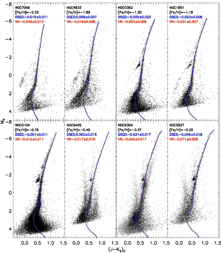
Figure 20.— Cluster photometry shifted to the absolute plane as in Fig. 7, with radial cuts applied in some cases as in Fig. 5. DSED (blue) and VR (red) models are overplotted, but after applying the fixed mean color offset from Table 5. These mean offsets and their standard deviation are given in each panel for each model.

The color offsets seen in the case of the DSED models are less drastic, and are confined to absolute values of $\Delta(J-K_{S})$ which fall well within the margin allowed by photometric error and calibration uncertainties. While it may be unsurprising that the D10 models require minimal color shifts since we adopted distances and reddenings based on the fits of these same models at optical wavelengths, our results serve as the first test of these models in the 2MASS filter system over the range of (age and metallicity) parameter space occupied by GGCs. For both the DSED and VR models, the largest (absolute) offset is seen for NGC 5927, the most metal-rich cluster in our sample. If we recalculate the offsets for this cluster assuming the value of $[Fe/H]$(D10, )=-0.5 rather than $[Fe/H]$(C09, )=-0.27 (shown as squares in Fig. 20), the discrepancy between models and data is brought into the range occupied by the remainder of the GGCs, but it is not resolved. Although our intention is not to sanction individual values for cluster parameters, such a downward revision of the NGC 5927 metallicity is suggested by the fits of Figs. 11, 12 and, to a marginal extent, Fig. 17. Also, Fig. 20 suggests that the DSED and VR models have essentially identical main sequence colors at fixed metallicity, and would continue to fall redward of the observed cluster MS in the near-IR at the extremes of the $[Fe/H]$ range sampled, although deeper photometry is needed to investigate this effect quantitatively. Lastly, it is possible that the color offsets between models and data could be resolved by a shift in cluster distances. However, throughout our investigation we have characterized the difference between models and data in terms of a color offset rather than a magnitude offset due to the verticality of the RGB in the near-IR. For example, even a modest color offset of $\Delta$$(J-K_{S})\sim$0.02 mag would require a shift of $\gtrsim$0.2 mag in the GGC distance scale.

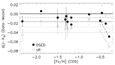
Figure 21.— Fixed mean color offsets applied to VR (grey open circles) and DSED models (black filled circles) in Fig. 20, shown as a function of cluster $[Fe/H]$ from C09 . Vertical error bars represent the standard deviation of the color difference between the model and observed ficucial sequence from Table 5. Offsets for NGC 5927 calculated using $[Fe/H]$(D10)=-0.5 rather than $[Fe/H]$(C09)=-0.27 are shown as open and filled squares for VR and DSED models respectively. The horizontal solid line represents equality, and horizontal dashed and dotted lines represent the median and median absolute deviation, respectively, of the color offset across all target clusters.

7. Summary and Conclusions

We have presented 2MASS-calibrated $J,K_{S}$ CMDs and fiducial sequences for 12 GGCs. These fiducial sequences have been used to produce relations between photometric indices which describe the shape of the upper RGB versus cluster metallicity, in terms of both $[Fe/H]$ and $[M/H]$. The resulting relations have slopes in excellent agreement with previous studies, and show zero point differences which can be attributed to uncertainties in the distance and reddening of the target clusters. While we have chosen to use cluster distances and reddenings based on isochrone fits by D10 to deep optical photometry, our relations are largely insensitive to current uncertainties in cluster distances, reddenings and metallicities for the more controversial cases. However, their precision as well as the size of the present sample could be improved by detailed spectroscopic abundances for a statistically representative quantity of cluster members, especially among the most metal-rich GGCs.

A comparison of empirical fiducial sequences to five sets of evolutionary models reveals that DSED and VR models most successfully reproduce the observed morphology of the RGB, although a color offset is needed to reconcile models and data. Although this offset is not formally significant compared to photometric errors as well as photometric calibration uncertainties (at least in the case of the DSED models), a comparison between the results of D10 and V13 suggests that it is unlikely to be caused solely by uncertainties in cluster distance and reddening values. Models also suggest that a modest ($\Delta$$Y$=0.04) helium enhancement negligibly affects the RGB morphology, although $\alpha$-enhancement plays a significant role, particularly on the upper RGB. This is in accord with our empirical relations, which generally give decreased rms residuals when fits are performed versus the global metallicity $[M/H]$ rather than $[Fe/H]$.

Relations between cluster metallicity and the near-IR magnitudes of the RGB bump and the HB (in the case of clusters with sufficiently red HBs) are also insensitive to the choice of recent cluster distances, reddenings, metallicities and ages beyond current uncertainties. Importantly, when using the LF peak to characterize the HB magnitude and its uncertainty, we find a non-negligible dependence between the near-IR HB magnitude and the cluster metallicity. This dependence, at the level of at least $\delta$$M_{K}(HB)/\delta$$[M/H]$=-0.4 mag/dex depending on the choice of cluster parameters, is larger than that predicted by the models of Salaris & Girardi (2002) and is robust to the choice of cluster distances, reddenings and ages.

The photometric catalogs and observed fiducial sequences presented here are being made publicly available, so that the our relations may be modified as the GGC distance and metallicity scales are improved. Similarly, it is our hope that the 2MASS-calibrated photometric catalogs may be of use as secondary standards for near-IR adaptive optics imagers on large telescopes, where saturation and/or a small field of view can impede photometric calibration.

References

- Anderson et al. (2008) Anderson, J. et al., 2008, AJ, 135, 2055
- Bergbusch & Stetson (2009) Bergbusch, P. A. & Stetson, P. B., 2009, AJ, 138, 1455
- Bessell & Brett (1988) Bessell, M. S. & Brett, J. M., 1988, PASP, 110, 1134
- Bono et al. (2010) Bono, G. et al., 2010, ApJ, 708, 74
- Brasseur et al. (2010) Brasseur, C., Stetson, P. B., VandenBerg, D. A., Casagrande, L., Bono, G. & Dall’Ora, M., 2010, AJ, 140, 1672
- Caloi, D’Antona & Mazzitelli (1997) Caloi, V., D’Antona, F. & Mazzitelli, I., 1997, A&A, 320, 823
- Carpenter (2001) Carpenter, J., 2001, AJ, 121, 2851
- Carretta & Gratton (1997) Carretta, E., & Gratton, R. G. 1997, A&AS, 121, 95
- Carretta et al. (2001) Carretta, E., Cohen, J. G., Gratton, R. G. & Behr, B. B., 2001, AJ, 122, 1469
- Carretta et al. (2007) Carretta, E., Recio-Blanco, A., Gratton, R. G., Piotto, G. & Bragaglia, A., 2007, ApJ, 671, 125
- (11) Carretta, E., Bragaglia, A., Gratton, R., D’Orazi, V. & Lucatello, S., 2009, A&A, 508, 695 (C09)
- Carretta et al. (2009b) Carretta, E., Bragaglia, A., Gratton, R. & Lucatello, S., 2009, A&A, 505, 139
- Carretta et al. (2009c) Carretta, E. et al., 2009, A&A, 505, 117
- Carretta et al. (2010a) Carretta, E., Bragaglia, A., Gratton, R. G., Recio-Blanco, A., Lucatello, S., D’Orazi, V. & Cassisi, S., 2010, A&A, 516, 55
- Carretta et al. (2010b) Carretta, E., Bragaglia, A., Gratton, R., Lucatello, S., Bellazzini, M. & D’Orazi, V., 2010, ApJ, 712, 21
- Carretta et al. (2014) Carretta, E. et al., 2014, A&A, 564, 60
- Casagrande & VandenBerg (2014) Casagrande, L. & VandenBerg, D. A., 2014, MNRAS, 444, 392
- Catelan (2009) Catelan, M., 2009, Ap&SS, 320, 261
- Cho & Lee (2002) Cho, D.-H. & Lee, S.-G., 2002, AJ, 124, 977
- Chun et al. (2010) Chun, S.-H. et al., 2010, A&A, 518, 15
- Clement et al. (2010) Clement, C. M. et al., 2001, AJ, 122, 2587
- Cohen & Sleeper (1995) Cohen, J. G. & Sleeper, C., 1995, AJ, 109, 242
- Cohen & Sarajedini (2012) Cohen, R. E. & Sarajedini, A., 2012, MNRAS, 419, 342
- Cohen et al. (2014) Cohen, R. E., Mauro, F., Geisler, D., Moni Bidin, C., Dotter, A. & Bonatto, C., 2014, AJ, 148, 18
- Demarque et al. (2004) Demarque, P., Woo, J.-H., Kim, Y.-C. & Yi, S. K., 2004, ApJS, 155, 667
- Dotter et al. (2008) Dotter, A., Chaboyer, B., Jevremovic, D., Kostov, V., Baron, E. & Ferguson, J. W., 2008, ApJS, 178, 89
- (27) Dotter, A. et al., 2010, ApJ, 708, 698 (D10)
- Ferraro et al. (1999) Ferraro, F. R., Valenti, E. & Origlia, L., 1999, ApJ, 649, 243
- Ferraro et al. (2000) Ferraro, F. R., Montegriffo, P., Origlia, L. & Fusi Pecci, F., 2000, AJ, 119, 1282
- Ferraro, Valenti & Origlia (2006) Ferraro, F. R., Valenti, E. & Origlia, L., 2006, ApJ, 649, 243
- Frogel, Cohen & Persson (1983) Frogel, J. A., Cohen, J. G. & Persson, S. E., 1983, AJ, 275, 773
- Goldsbury et al. (2010) Goldsbury, R., Richer, H. B., Anderson, J., Dotter, A., Sarajedini, A., Woodley, K., 2010, AJ, 140, 1830
- Gonzalez et al. (2011) Gonzalez, O. A., Rejkuba, M., Zoccali, M., Valenti, E., Minniti, D., Schultheis, M., Tobar, R., & Chen, B., 2012, A&A, 543, 13
- Gonzalez et al. (2013) Gonzalez, O. A., Rejkuba, M., Zoccali, M., Valenti, E., Minniti, D., Tobar, R., 2013, A&A, 552, 110
- Górski et al. (2011) Górski, M., Pietrzyński, G., & Gieren, W. 2011, AJ, 141, 194
- Gratton et al. (2010) Gratton, R. G., Lucatello, S., Carretta, E. Bragaglia, A., D’Orazi, V. & Momany, Y. A., 2011, A&A, 534, 123
- Gratton et al. (2010) Gratton, R. G., Carretta, E., Bragaglia, A., Lucatello, S. & D’Orazi, V., 2010, A&A, 517, 81
- Grocholski & Sarajedini (2002) Grocholski, A. J. & Sarajedini, A., 2002, AJ, 123, 1602
- Harris (1996) Harris, W. E., 1996, AJ, 112, 1487
- Hayden et al. (2015) Hayden, M. et al., 2015, arXiv:1503.02110
- Held et al. (2010) Held, E. V., Gullieuszik, M., Rizzi, L., Girardi, L. Marigo, P. & Saviane, I., 2010, MNRAS, 404, 1475
- Hempel et al. (2014) Hempel, M. et al., 2014, ApJS, 211, 1
- Hendricks et al. (2012) Hendricks, B., Stetson, P. B., VandenBerg, D. A. & Dall’Ora, M., 2012, AJ, 144, 25
- Ivanov & Borissova (2002) Ivanov, V. D. & Borissova, J., 2002, A&A, 390, 937
- Kim et al. (2006) Kim, J.-W. et al., 2006, A&A, 459, 499
- Krogsrud et al. (2013) Krogsrud, D. A., Sandquist, E. J. & Kato, T., 2013, ApJ, 767, LL27
- Marin-Franch et al. (2009) Marin-Franch, A. et al., 2009, ApJ, 694, 1498
- Mauro et al. (2013) Mauro, F., Moni Bidin, C., Chené, A.-N. et al., 2013, RMxAA, 49, 189
- Mauro et al. (2014) Mauro, F., Moni Bidin, C., Geisler, D. et al., 2014, A&A, 563, 76
- Milone et al. (2014) Milone, A. P. et al., 2014, ApJ, 785, 21
- Montegriffo et al. (1998) Montegriffo, P., Ferraro, F. R., Origlia, L. & Fusi Pecci, F., 1998, MNRAS, 297, 872
- Nataf et al. (2011) Nataf, D. M., Gould, A., Pinsonneault, M. H. & Stetson, P. B., 2011, ApJ, 736, 94
- Nataf et al. (2013) Nataf, D. M., Gould, A. P., Pinsonneault, M. H. & Udalski, A., 2013, ApJ, 766, 77
- Pietrinferni et al. (2006) Pietrinferni, A., Cassisi, S., Salaris, M. & Castelli, F., 2006, ApJ, 642, 797
- Piotto et al. (2002) Piotto, G. et al., 2002, A&A, 391, 945
- Piotto et al. (2014) Piotto, G. et al., 2014, arXiv:1410.4654
- Roederer & Thompson (2015) Roederer, I. U. & Thompson, I. B., 2015, arXiv:1503.03079
- Rosenberg et al. (1999) Rosenberg, A., Saviane, I., Piotto, G. & Aparicio, A., 1999, AJ, 118, 2306
- Salaris et al. (1993) Salaris, M., Chieffi, A. & Straniero, O., 1993, ApJ, 414, 580
- Salaris & Cassisi (1997) Salaris, M. & Cassisi, S., 1997, MNRAS, 289, 406
- Salaris & Girardi (2002) Salaris, M. & Girardi, L., 2002, MNRAS, 337, 332
- Salaris et al. (2007) Salaris, M., Held, E. V., Ortolani, S., Gullieuszik, M. & Momany, Y., 2007, A&A, 476, 243
- Sarajedini et al. (2007) Sarajedini, A. et al., 2007, AJ, 133, 1658
- Sirianni et al. (2005) Sirianni, M. et al., 2005, PASP, 117, 1049
- Skrutskie et al. (2006) Skrutskie, M. F., Cutri, R. M., Stiening, R., Weinberg, M. D., Schneider, S. et al, 2006, AJ, 131, 1163
- Sobeck et al. (2006) Sobeck, J. S., Ivans, I. I., Simmerer, J. A., Sneden, C., Hoeflich, P., Fulbright, J. P . & Kraft, R. P., 2006, AJ, 131, 2949
- Stetson (1987) Stetson, P. B., 1987, PASP, 99, 191
- Stetson (1994) Stetson, P. B., 1994, PASP, 106, 250
- Stetson (2000) Stetson, P. B., 2000, PASP, 112, 925
- Straniero, Chieffi & Limongi (1997) Staniero, O., Chieffi, A. & Limongi, M., 1997, ApJ, 490, 425
- Valcarce, Catelan & Sweigart (2012) Valcarce, A. A. R., Catelan, M., & Sweigart, A. V. 2012, A&A, 547, AA5
- Valenti et al. (2004a) Valenti, E., Ferraro, F. R. & Origlia, L., 2004, MNRAS, 351, 1204
- Valenti et al. (2004b) Valenti, E., Ferraro, F. R. & Origlia, L., 2004, MNRAS, 354, 815
- Valenti et al. (2005) Valenti, E., Origlia, L. & Ferraro, F. R., 2005, MNRAS, 361, 272
- Valenti et al. (2010) Valenti, E., Ferraro, F. R. & Origlia, L., 2010, MNRAS, 402, 1729
- VandenBerg (2013) VandenBerg, D. A., 2013, IAU Symposium, 289, 161
- (77) VandenBerg, D. A., Brogaard, K., Leaman, R. & Casagrande, L., 2013, ApJ, 775, 134 (V13)
- VandenBerg et al. (2014) VandenBerg, D. A., Bergbusch, P. A., Ferguson, J. W. & Edvardsson, B., 2014, ApJ, 794, 72
- Vanderbeke et al. (2015) Vanderbeke, J., De Propris, R., De Rijcke, S., Baes, M., West, M., Alonso-Garcia, J. & Kunder, A., 2015, arXiv:1504.06509
- Yi, Kim & Demarque (2003) Yi, S. K., Kim, Y.-C. & Demarque, P., 2003, ApJS, 144, 259
- Zoccali et al. (2004) Zoccali, M., Barbuy, B., Hill, V. et al., 2004, A&A, 423, 507