Approximation of fuzzy numbers by convolution method

Abstract

In this paper we consider how to use the convolution method to construct approximations, which consist of fuzzy numbers sequences with good properties, for a general fuzzy number. It shows that this convolution method can generate differentiable approximations in finite steps for fuzzy numbers which have finite non-differentiable points. In the previous work, this convolution method only can be used to construct differentiable approximations for continuous fuzzy numbers whose possible non-differentiable points are the two endpoints of 1-cut. The constructing of smoothers is a key step in the construction process of approximations. It further points out that, if appropriately choose the smoothers, then one can use the convolution method to provide approximations which are differentiable, Lipschitz and preserve the core at the same time.

1 Instructions

The approximations of fuzzy numbers attract many people’s attention. Mostly, the researches can be grouped into two classes. One class is to use a given shape fuzzy number to approximate the original fuzzy number. There exist many important works which include but not limited to the following. Chanas [5] and Grzegorzewski [14] independently presented the interval approximations. Ma et al. [20] presented the symmetric triangular approximations. Abbasbandy and Asady [1] presented the trapezoidal approximations. Grzegorzewski and Mrówka [15, 16] presented the trapezoidal approximations preserving the expected interval. Zeng and Li [29] presented the weighted triangular approximations. Nasibov and Peker [21] presented the semi-trapezoidal approximations which is improved by Ban [2, 3]. Yeh [25] presented the weighted semi-trapezoidal approximations. Yeh and Chu [26] presented a unified method to solve the LR-type approximation problems without constraints according to the weighted $L_{2}$-metric. Coroianu [10] discussed how to find the best Lipschitz constant of the trapezoidal approximation operator preserving the value and ambiguity. Ban and Coroianu [4] proposed simpler methods to compute the parametric approximation of a fuzzy number preserving some important characteristics. The works of this class of fuzzy numbers approximation provide various methods to approximate an arbitrary fuzzy number according to some metrics by a special type of fuzzy number which is much more convenient to be calculated. At the same time, since it finds the fuzzy number which has the minimal distance to the original fuzzy number among all the given type fuzzy numbers, it minimizes the loss of the information to a certain extent.

But there exist many situations in which the smaller the distance between approximated fuzzy number and original fuzzy number becomes, the better the effect appears. So it is also important to consider the problem whether one can approximate a fuzzy number arbitrary well by fuzzy numbers with some good properties such as continuous, differentiable, etc. This is the topic of another class of researches for fuzzy number approximation which discuss how to construct a fuzzy numbers sequence with some properties to approximate a general fuzzy number. There also exist many important contributions including the following works. Colling and Kloeden [7] used the continuous fuzzy numbers sequence to approximate an arbitrary fuzzy number. Coroianu et al. [8, 9] constructed approximations which is made up of fuzzy numbers sequence by using the F-transform and the max-product Bernstein operators, respectively. Román-Flores et al. [22] pointed out a fact that the Lipschitzian fuzzy numbers sequences can approximate any fuzzy numbers. To demonstrate this fact, they presented a method based on the convolution of two fuzzy numbers to construct approximations for fuzzy numbers. For writing convenience, we call this method convolution method in the sequel. This convolution method traces back to the work of Seeger and Volle [23].

Differentiable fuzzy numbers play an important role in the implementation of fuzzy intelligent systems and their applications (see [6, 17]). For instance, to use the well-known gradient descent algorithm, it needs the fuzzy numbers be differentiable. So it is an important and vital question that whether one can use the differentiable fuzzy numbers sequence to approximate a general fuzzy number. Chalco-Cano et al. [27, 28] used the convolution method to construct differentiable fuzzy numbers sequences to approximate a type of non-differentiable fuzzy numbers under supremum metric. Since the convergence induced by supremum metric is stronger than the convergences induced by $L_{p}$-metric, sendograph metric, endograph metric, and level-convergence (see [11, 24, 18, 19]), it follows that the constructed approximation is also an approximation for the original fuzzy number under the above mentioned convergences. This method is easy to be implemented since its operation is on level-cut-sets of the fuzzy numbers. In the sequel, a differentiable fuzzy number is also called a smooth fuzzy number, a non-differentiable fuzzy number is called a non-smooth fuzzy number, and an approximation which consists of differentiable fuzzy numbers sequence is called a smooth approximation.

To construct smooth approximations for a type of non-smooth fuzzy numbers, Chalco-Cano et al.[27, 28] showed an interesting fact that the convolution transform can be used to smooth this type of fuzzy numbers, i.e. it can transfer a non-smooth fuzzy number in this type to a smooth fuzzy number. In fact, they constructed a class of ‘smoothers’ which are fuzzy numbers satisfying some conditions. Given a non-smooth fuzzy number of this type, it can obtain a smooth fuzzy number via convolution of the original fuzzy number and the smoother. The construction of smoothers is an important step in the construction of approximations. The distance between the smooth fuzzy number and the original fuzzy number can be controlled by the smoother. Thus, by appropriately choosing the smoother, it can get a smooth fuzzy number such that the distance between which and the original fuzzy number is less than an arbitrarily small positive number given in advance. So it can produce a sequence of smooth fuzzy numbers which constitute a smooth approximation of the original fuzzy numbers.

However, in the previous work, only a given type of fuzzy numbers can be smoothed by the convolution method. Hence only this type of fuzzy numbers can be smoothly approximated by using the convolution method. This type of fuzzy numbers have at most two possible non-differentiable points which are the endpoints of 1-cut. Whereas, an arbitrary fuzzy number may have other non-differentiable points, or even non-continuous points. So it is natural to consider the question whether one can use the convolution method to smooth a general fuzzy number and then the question whether one can give a smooth approximation to the original fuzzy number.

In this paper, we want to answer these questions. For this purpose, we first discuss the properties of fuzzy numbers and convolution of fuzzy numbers. Based on these discussions, we give partial positive answers to above questions. The key is how to construct smoothers for a general fuzzy number so that it can be smoothed. We do this step by step. It first shows how to construct smoothers for a subtype of continuous fuzzy numbers. Then it investigates how to construct smoothers for the continuous fuzzy numbers. At last, it explores how to construct smoothers for an arbitrary fuzzy number so that it can be transformed into a smooth fuzzy number. On the basis of above results, it shows that how to construct smooth approximations for fuzzy numbers which have finite non-differentiable points. This type of fuzzy numbers are quite general in real world applications. It further finds that, by appropriately choosing the smoothers, the smooth approximations can be Lipschitz approximations and can preserve the core at the same time. We give simulation examples to validate and to illustrate the theoretical results.

The remainder of this paper is organized as follows. Section 2 presents preliminaries about fuzzy numbers and the convolution method for approximating fuzzy numbers. Section 3 gives properties on the continuity of fuzzy numbers. In Section 4, it shows that the convolution transform can keep the differentiability of fuzzy numbers which is the key property to ensure that the convolution method can be used to smooth fuzzy numbers. On the basis of the results in Sections 3 and 4, it discusses how to smooth and approximate a general fuzzy number in Section 5. In Section 6, it investigates advantages of constructing approximations by the convolution method. In Section 7, we draw conclusions.

2 Preliminaries

2.1 Fuzzy numbers

In this subsection, we introduce some basic and important notations and properties about fuzzy numbers which will be used in the sequel. For details, we refer the reader to references [11, 24].

Let $\mathbb{N}$ be the set of all natural numbers, $\mathbb{R}$ be the set of all real numbers. A fuzzy subsets $u$ on $\mathbb{R}$ can be seen as a mapping from $\mathbb{R}$ to [0,1]. For $\alpha\in(0,1]$, let $[u]_{\alpha}$ denote the $\alpha$-cut of $u$; i.e.,  $[u]_{\alpha}\equiv\{x\in\mathbb{R}:u(x)\geq\alpha\}$ and $[u]_{0}$ denotes $\overline{\{x\in\mathbb{R}:u(x)>0\}}$. We call $u$ a fuzzy number if $u$ has the following properties:
(i) $[u]_{1}\neq\emptyset$; and
(ii) $[u]_{\alpha}=[u^{-}(\alpha),u^{+}(\alpha)]$ are compact intervals of $\mathbb{R}$ for all $\alpha\in[0,1]$.
The set of all fuzzy numbers is denoted by $\mathcal{F}(\mathbb{R})$. In [27], a fuzzy number is also called a fuzzy interval.

Suppose that $u$ is a fuzzy number. The 1-cut of $u$ is also called the core of $u$, which is denoted by Core($u$), i.e. Core($u)=[u]_{1}$. $u$ is said to be Lipschitz if $u$ is a Lipschitz function on $[u]_{0}$, i.e. $|u(x)-u(y)|\leq K|x-y|$ for all $x,y\in[u]_{0}$, where $K$ is a constant which is called the Lipschitz contant.

The following is a widely used representation theorem of fuzzy numbers.

Proposition 2.1

(Goetschel and Voxman [13]) Given $u\in\mathcal{F}(\mathbb{R}),$ then

(i)  $u^{-}(\cdot)$ is a left-continuous nondecreasing bounded function on $(0,1]$;
(ii)  $u^{+}(\cdot)$ is a left-continuous nonincreasing bounded function on $(0,1]$;
(iii)  $u^{-}(\cdot)$ and $u^{+}(\cdot)$ are right continuous at $\alpha=0$;
(iv)  $u^{-}(1)\leq u^{+}(1).$

Moreover, if the pair of functions $a(\lambda)$ and $b(\lambda)$ satisfy conditions (i) through (iv), then there exists a unique $u\in\mathcal{F}(\mathbb{R})$ such that $[u]_{\alpha}=[a(\lambda),b(\lambda)]$ for each $\alpha\in(0,1].$

From the definition of fuzzy numbers, we know that, given $x<u^{-}(1)$, then $u(x)=\lim_{z\to x+}u(z)$, i.e. $u$ is right-continuous at $x<u^{-}(1)$. Similarly, $u(x)=\lim_{z\to x-}u(z)$ for each $x>u^{+}(1)$, i.e., $u$ is left-continuous at each $x>u^{+}(1)$.

The algebraic operations on $\mathcal{F}(\mathbb{R})$ are defined as follows: given $u,\ v\in\mathcal{F}(\mathbb{R})$, $\alpha\in[0,1]$,

$$[u+v]_{\alpha}=[u]_{\alpha}+[v]_{\alpha}=[u^{-}(\alpha)+v^{-}(\alpha),\ u^{+}(\alpha)+v^{+}(\alpha)],$$

$$[u-v]_{\alpha}=[u]_{\alpha}-[v]_{\alpha}=[u^{-}(\alpha)-v^{+}(\alpha),\ u^{+}(\alpha)-v^{-}(\alpha)],$$

$$[u\cdot v]_{\alpha}=[u]_{\alpha}\cdot[v]_{\alpha}=[\min\{xy:\;x\in[u]_{\alpha},\,y\in[v]_{\alpha}\},\ \max\{xy:\;x\in[u]_{\alpha},\,y\in[v]_{\alpha}\}].$$ (1)

From (1), we know that if $r$ is a real number and $v$ is a fuzzy number, then

$$(r\cdot v)(t)=\left\{\begin{array}[]{ll}v(t/r),&\ r\not=0,\\ \chi_{\{0\}}(t),&\ r=0,\end{array}\right.$$

where $\chi_{\{0\}}$ is the characterization of $\{0\}$.

Suppose that $u$ is a fuzzy number. Its strong-$\alpha$-cuts $[u]_{\alpha}^{s}$, $\alpha\in[0,1]$, are defined by:

$$[u]_{\alpha}^{s}=[u_{s}^{-}(\alpha),u_{s}^{+}(\alpha)]=\left\{\begin{array}[]{ll}\overline{\bigcup_{\beta>\alpha}[u]_{\beta}}=[\lim_{\beta\to\alpha+}u^{-}(\beta),\lim_{\beta\to\alpha+}u^{+}(\beta)],&\ \alpha<1,\\ \mbox{}[u]_{1}=[u^{-}(1),u^{+}(1)],&\ \alpha=1.\end{array}\right.$$

Clearly, $[u]_{1}=[u]^{s}_{1}$, $[u]_{0}=[u]^{s}_{0}$, and $[u]^{s}_{\alpha}\subseteq[u]_{\alpha}$ for all $\alpha\in[0,1]$. It is easy to show that

$$[u+v]^{s}_{\alpha}=[u]^{s}_{\alpha}+[v]^{s}_{\alpha}=[u^{-}_{s}(\alpha)+v^{-}_{s}(\alpha),\ u^{+}_{s}(\alpha)+v^{+}_{s}(\alpha)],$$

$$[u-v]^{s}_{\alpha}=[u]^{s}_{\alpha}-[v]^{s}_{\alpha}=[u^{-}_{s}(\alpha)-v^{+}_{s}(\alpha),\ u^{+}_{s}(\alpha)-v^{-}_{s}(\alpha)].$$

We call $u^{-}(\cdot),\ u^{+}(\cdot),\ u_{s}^{-}(\cdot),\ u_{s}^{+}(\cdot)$ cut-functions. The $\alpha$-cut and strong-$\alpha$-cut are also called level-cut-set or strong-level-cut-set, respectively.

The supremum metric on $\mathcal{F}(\mathbb{R})$ is defined by

$$d_{\infty}(u,v)=\sup_{\alpha\in[0,1]}\max\{|u^{-}(\alpha)-v^{-}(\alpha)|,\ |u^{+}(\alpha)-v^{+}(\alpha)|\},$$

where $u,v\in\mathcal{F}(\mathbb{R}).$

2.2 Convolution method for approximating fuzzy numbers

This subsection describes a method based on the convolution transform to approximate a fuzzy number. This convolution method was first putted forward by Román-Flores [22], and traced back to the work of Seeger and Volle [23]. Chalco-Cano et al. [27, 28] gave important contributions to this method. They used this convolution method to produce smooth approximations for a class of non-smooth fuzzy numbers.

The sup-min convolution $u\nabla v$ of fuzzy numbers $u$ and $v$ is defined by

$$(u\nabla v)(x)=\sup_{y\in\mathbb{R}}\{u(y)\wedge v(x-y)\}.$$

Remark 2.2

In fact $u\nabla v=u+v$ for all $u,v\in\mathcal{F}(\mathbb{R})$. For details, see [11, 24].

The following is some symbols which are used to denote subsets of $\mathcal{F}(\mathbb{R})$.

• $\mathcal{F}_{\mathrm{T}}(\mathbb{R})$ is denoted the family of all fuzzy numbers $u$ such that $u$ is strictly increasing on $[u^{-}(0),u^{-}(1)]$, strictly decreasing on $[u^{+}(1),u^{+}(0)]$, and differentiable on $(u^{-}(0),u^{-}(1))\cup(u^{+}(1),u^{+}(0))$.

• $\mathcal{F}_{\mathrm{N}}(\mathbb{R})$ is denoted the family of all fuzzy numbers $u$ such that $u$ is differentiable on $(u^{-}(0),u^{-}(1))\cup(u^{+}(1),u^{+}(0))$.

• $\mathcal{F}_{\mathrm{C}}(\mathbb{R})$ is denoted the family of all fuzzy numbers $u$ such that $u:\mathbb{R}\to[0,1]$ is continuous on $[u]_{0}=[u^{-}(0),u^{+}(0)]$. In other words, given $u\in\mathcal{F}(\mathbb{R})$ with $[u]_{0}$ is not a singleton, then $u\in\mathcal{F}_{\mathrm{C}}(\mathbb{R})$ if and only if $u$ is continuous on $(u^{-}(0),u^{+}(0))$, right-continuous on $u^{-}(0)$ and left-continuous on $u^{+}(0)$.

• $\mathcal{F}_{\mathrm{D}}(\mathbb{R})$ is denoted the family of all differentiable fuzzy numbers, i.e., the family of all fuzzy numbers $u\in\mathcal{F}_{\mathrm{C}}(\mathbb{R})$ such that $u:\mathbb{R}\to[0,1]$ is differentiable on $(u^{-}(0),u^{+}(0))$.

Given a fuzzy number $u$ in $\mathcal{F}_{\mathrm{N}}(\mathbb{R})$, $u$ need not be strictly increasing on $(u^{-}(0),u^{-}(1))$ and strictly decreasing on $(u^{+}(1),u^{+}(0))$. So

$$\mathcal{F}_{\mathrm{T}}(\mathbb{R})\subsetneq\mathcal{F}_{\mathrm{N}}(\mathbb{R}).$$

Observe that, for each $v\in\mathcal{F}(\mathbb{R})$, $v$ is differentiable on $(v^{-}(1),v^{+}(1))$. Thus, for every $u\in\mathcal{F}_{\mathrm{N}}(\mathbb{R})$, its possible non-differentiable points in $(u^{-}(0),u^{+}(0))$ are $u^{-}(1)$ and $u^{+}(1)$. It is easy to check that

$$\mathcal{F}_{\mathrm{D}}(\mathbb{R})\subsetneq\mathcal{F}_{\mathrm{C}}(\mathbb{R})\cap\mathcal{F}_{\mathrm{N}}(\mathbb{R}).$$

Clearly, given $u\in\mathcal{F}_{\mathrm{D}}(\mathbb{R})$, if $x\in[u]_{1}$ and $x$ is an inner point of $[u]_{0}$, then $u^{\prime}(x)=0$. We also call $u\in\mathcal{F}_{\mathrm{D}}(\mathbb{R})$ a smooth fuzzy number.

Suppose that $u\in\mathcal{F}(\mathbb{R})$ and $v\in\mathcal{F}_{\mathrm{D}}(\mathbb{R})$, then $v$ is said to be a smoother of $u$ if $u\nabla v\in\mathcal{F}_{\mathrm{D}}(\mathbb{R})$.

Chalco-Cano et al. [27] pointed out that each fuzzy number in $\mathcal{F}_{\mathrm{T}}(\mathbb{R})$ can be approximated by a smooth fuzzy numbers sequence which is constructed by using the convolution method. They constructed fuzzy numbers $w_{p}$, $p>0$, as follows:

$$w_{p}(x)=\left\{\begin{array}[]{ll}1-{\left(\frac{x}{p}\right)}^{2},&\mbox{if}\ x\in[-p,p],\\ 0,&\mbox{if}\ x\notin[-p,p].\end{array}\right.$$ (2)

Obviously, $w_{p}\in\mathcal{F}_{\mathrm{D}}(\mathbb{R})$ for all $p>0$. They presented the following result.

Proposition 2.3

[27] If $u\in\mathcal{F}_{\mathrm{T}}(\mathbb{R})$, then $u\nabla w_{p}\in\mathcal{F}_{\mathrm{D}}(\mathbb{R})$.

Notice that $d_{\infty}(u,u\nabla w_{p})\to 0$ as $p\to 0$. Thus Proposition 2.3 indicates that every fuzzy number in $\mathcal{F}_{\mathrm{T}}(\mathbb{R})$ can be approximated by fuzzy numbers sequences contained in $\mathcal{F}_{\mathrm{D}}(\mathbb{R})$.

We can see that the fuzzy numbers $w_{p}$, $p>0$, work as smoothers, which transfer each fuzzy number $u$ to a smooth fuzzy number $u\nabla w_{p}$. The smooth fuzzy numbers sequence $\{u\nabla w_{p}\}$ construct a smooth approximation of the original fuzzy number $u$, i.e., $u\nabla w_{p}\to u$ as $p\to 0$.

Chalco-Cano et al. [28] further presented an approach to produce a more large class of smoothers. A class of fuzzy numbers $Z_{p}^{f}$ are defined by

$$Z_{p}^{f}(x)=\begin{cases}f^{-1}(\|x\|/p),&\|x\|\leq p,\\ 0,&\|x\|>p,\end{cases}$$ (3)

where $p>0$ is a real number and that $f:[0,1]\to[0,1]$ is a continuous and strictly decreasing function with $f(0)=1,f(1)=0$. It is easy to see that $Z_{p}^{f}=w_{p}$ when $f=\sqrt{1-t}$. They gave the following result.

Proposition 2.4

[28] Suppose that $Z_{p}^{f}$ is defined by (3). If $f$ is differentiable and $\lim_{\alpha\to 1-}f^{\prime}(\alpha)=-\infty$, then $u\nabla Z_{p}^{f}\in\mathcal{F}_{\mathrm{D}}(\mathbb{R})$ for each $u\in\mathcal{F}_{\mathrm{T}}(\mathbb{R})$.

Notice that $d_{\infty}(u\nabla Z_{p}^{f},\ u)\to 0$ as $p\to 0$. This means that given $f$ satisfies the above conditions, it produces a class of smoothers $\{Z_{p}^{f}:\ p>0\}$ and a smooth approximation $\{u\nabla Z_{p}^{f}:\ p>0\}$ of the fuzzy number $u$. Different $f$ corresponds to different class of smoothers and then corresponds to different smooth approximation.

3 Properties of fuzzy numbers

In this section, we investigate some properties on the continuity of fuzzy numbers which will be used in the sequel. It first lists some conclusions on the values of membership functions of fuzzy numbers, and conclusions on characterizations of continuous points of fuzzy numbers. Based on this, it gives some characterizations of continuous intervals of fuzzy numbers. At last, it considers the properties of continuous points of the cut-functions of fuzzy numbers.

We list some propositions and corollary which can be found in [11, 24] or as direct consequences of the conclusions therein. The following four conclusions discuss values of fuzzy numbers’ membership functions.

Proposition 3.1

Suppose that $u\in F(\mathbb{R})$ and that $x\in\mathbb{R}$, then the following statements hold.
(i)  If $u^{-}(1)\geq x>u_{s}^{-}(\alpha)$, then $u(x)>\alpha$.
(ii)  If $u^{+}(1)\leq x<u_{s}^{+}(\alpha)$, then $u(x)>\alpha$.
(iii)  If $x<u_{s}^{-}(\alpha)$ or $x>u_{s}^{+}(\alpha)$, then $u(x)\leq\alpha$.

Proposition 3.2

Suppose that $u\in F(\mathbb{R})$ and that $x\in\mathbb{R}$, then the following statements hold.
(i)  If $u^{-}(\alpha)<u^{-}_{s}(\alpha)$, then $u(x)=\alpha$ when $x\in(u^{-}(\alpha),u^{-}_{s}(\alpha))$.
(ii)  If $u^{+}(\alpha)>u^{+}_{s}(\alpha)$, then $u(x)=\alpha$ when $x\in(u^{+}_{s}(\alpha),u^{+}(\alpha))$.

Proposition 3.3

Suppose that $u\in\mathcal{F}(\mathbb{R})$. If $u$ is continuous at a point $x\in(u^{-}(0),u^{+}(0))$ which is equal to $u^{-}(\alpha)$ or $u^{+}(\alpha)$ or $u_{s}^{-}(\alpha)$ or $u_{s}^{+}(\alpha)$, then $u(x)=\alpha$.

Corollary 3.4

If $u\in\mathcal{F}_{\mathrm{C}}(\mathbb{R})$, then

$$u(u^{-}(\alpha))=u(u_{s}^{-}(\alpha))=\alpha,$$

$$u(u^{+}(\beta))=u(u_{s}^{+}(\beta))=\beta$$

for all $\alpha\geq u(u^{-}(0))$ and $\beta\geq u(u^{+}(0))$.

Propositions 3.5 and 3.6 consider characterizations of continuous points of a fuzzy number.

Proposition 3.5

Suppose that $u\in\mathcal{F}(\mathbb{R})$, then the following statements hold.
(i)   Given $x\in(u^{-}(0),u^{+}(1)]$, then $u$ is left-continuous at $x$ if and only if $u^{-}(\beta)<x$ for each $\beta<u(x)$.
(ii)   Given $x\in[u^{-}(1),u^{+}(0))$, then $u$ is right-continuous at $x$ if and only if $u^{+}(\beta)>x$ for each $\beta<u(x)$.

Proposition 3.6

Suppose that $u\in\mathcal{F}(\mathbb{R})$. Then the following statements hold.
(i)  Given $u^{-}(\alpha)\in(u^{-}(0),u^{-}(1))$, then $u$ is continuous at $u^{-}(\alpha)$ if and only if $u(u^{-}(\alpha))=\alpha$, and $u^{-}(\beta)<u^{-}(\alpha)$ for each $\beta<\alpha$.
(ii)  Given $u_{s}^{-}(\alpha)\in(u^{-}(0),u^{-}(1))$, then $u$ is continuous at $u_{s}^{-}(\alpha)$ if and only if $u(u_{s}^{-}(\alpha))=\alpha$, and $u^{-}(\beta)<u_{s}^{-}(\alpha)$ for each $\beta<\alpha$.
(iii)  Given $u^{+}(\alpha)\in(u^{+}(1),u^{+}(0))$, then $u$ is continuous at $u^{+}(\alpha)$ if and only if $u(u^{+}(\alpha))=\alpha$, and $u^{+}(\beta)>u^{+}(\alpha)$ for each $\beta<\alpha$.
(iv)  Given $u^{+}_{s}(\alpha)\in(u^{+}(1),u^{+}(0))$, then $u$ is continuous at $u_{s}^{+}(\alpha)$ if and only if $u(u_{s}^{+}(\alpha))=\alpha$, and $u^{+}(\beta)>u_{s}^{+}(\alpha)$ for each $\beta<\alpha$.

The following lemmas and theorems give characterizations of continuous intervals of a fuzzy number.

Lemma 3.7

Suppose that $u\in\mathcal{F}(\mathbb{R})$. Given $a,b\in[u^{-}(0),u^{-}(1)]$ with $a<b$, then the following statements are equivalent.
(i) There exists $x$ in $(a,b]$ such that $u$ is not left-continuous at $x$.
(ii) There exists $\alpha,\beta$ in $[u(a),u(b)]$ such that $\alpha\not=\beta$ and $u^{-}(\alpha)=u^{-}(\beta)$.
(iii) $u^{-}(\cdot)$ is not strictly increasing on $[u(a),u(b)]$.

Proof  If statement (i) holds, then there exists $x\in(a,b]$ such that $u$ is not left-continuous at $x$. Hence $\alpha=u(x)>\lim_{z\to x-}u(z)=\beta$, and thus $u^{-}(\alpha)=u^{-}(\frac{\alpha+\beta}{2})=x$. Note that $\alpha\not=\frac{\alpha+\beta}{2}$ and $\alpha,\beta\in[u(a),u(b)]$. So statement (ii) holds.

If statement (ii) holds, then there exist $\alpha>\beta$ such that $u^{-}(\alpha)=u^{-}(\beta)=x$ and $\alpha,\beta\in[u(a),u(b)]$. So $\lim_{z\to x-}u(z)\leq\beta<\alpha\leq u(x)$. This means that $u$ is not left-continuous at $x\in(a,b]$, i.e., statement (i) holds.

The equivalence of statement (ii) and statement (iii) follows immediately from the monotonicity of $u^{-}(\cdot)$. $\quad\Box$

Lemma 3.8

Suppose that $u\in\mathcal{F}(\mathbb{R})$. Given $c,d\in[u^{+}(1),u^{+}(0)]$ with $c<d$, then the following statements are equivalent.
(i) There exists $x$ in $[c,d)$ such that $u$ is not right-continuous at $x$.
(ii) There exists $\alpha,\beta$ in $[u(c),u(d)]$ such that $\alpha\not=\beta$ and $u^{+}(\alpha)=u^{+}(\beta)$.
(iii) $u^{+}(\cdot)$ is not strictly decreasing on $[u(c),u(d)]$.

Proof  The proof is similar to the proof of Lemma 3.7. $\quad\Box$

Theorem 3.9

Suppose that $u\in\mathcal{F}(\mathbb{R})$. Then $u\in\mathcal{F}_{\mathrm{C}}(\mathbb{R})$ if and only if the following two conditions are satisfied.
(i)  $u^{-}(\alpha)\not=u^{-}(\beta)$ for all $\alpha,\beta\in[u(u^{-}(0)),1]$ with $\alpha\not=\beta$.
(ii)  $u^{+}(\alpha)\not=u^{+}(\beta)$ for all $\alpha,\beta\in[u(u^{+}(0)),1]$ with $\alpha\not=\beta$.

Proof  If $[u]_{0}$ is a singleton, the the conclusion holds obviously. If $[u]_{0}$ is not a singleton, the desired results follow from Lemmas 3.7 and 3.8. $\quad\Box$

Theorem 3.10

Suppose that $u\in\mathcal{F}(\mathbb{R})$ and that $u(u^{-}(0))=\alpha_{0}$ and $u(u^{+}(0))=\beta_{0}$. Then $u\in\mathcal{F}_{\mathrm{C}}(\mathbb{R})$ if and only if $u^{-}(\cdot)$ is strictly increasing on $[\alpha_{0},1]$ and $u^{+}(\cdot)$ is strictly decreasing on $[\beta_{0},1]$.

Proof   Suppose that $u\in\mathcal{F}_{\mathrm{C}}(\mathbb{R})$, it then follows from Lemmas 3.7 and 3.8 that $u^{-}(\cdot)$ is strictly increasing on $[\alpha_{0},1]$ and $u^{+}(\cdot)$ is strictly decreasing on $[\beta_{0},1]$.

Suppose that $u^{-}(\cdot)$ is strictly increasing on $[\alpha_{0},1]$ and $u^{+}(\cdot)$ is strictly decreasing on $[\beta_{0},1]$. Given $u\in\mathcal{F}(\mathbb{R})$ with $[u]_{0}$ is not a singleton, then $u^{-}(0)<u^{-}(1)$ or $u^{-}(0)=u^{-}(1)<u^{+}(1)$ or $u^{-}(0)=u^{-}(1)=u^{+}(1)<u^{+}(0)$. We can check that in all above cases, $u$ is right-continuous on $u^{-}(0)$. Similarly, we know that $u$ is left-continuous on $u^{+}(0)$. By using Lemmas 3.7 and 3.8, we can also check that $u$ is continuous on $(u^{-}(0),u^{+}(0))$. Combined with above conclusions, we know that $u\in\mathcal{F}_{\mathrm{C}}(\mathbb{R})$. $\quad\Box$

Lemma 3.11

Suppose that $u,v\in\mathcal{F}(\mathbb{R})$ and that $\alpha\in[0,1]$, then

$$(u\nabla v)((u\nabla v)^{-}(\alpha))=u(u^{-}(\alpha))\wedge v(v^{-}(\alpha)),$$

$$(u\nabla v)((u\nabla v)^{+}(\alpha))=u(u^{+}(\alpha))\wedge v(v^{+}(\alpha)).$$

Proof  From Zadeh’s extension principle, we know that

$$(u\nabla v)((u\nabla v)^{-}(\alpha))$$

$$=\sup\{u(x)\wedge v(y):x+y=(u\nabla v)^{-}(\alpha)=u^{-}(\alpha)+v^{-}(\alpha)\}$$

$$\geq u(u^{-}(\alpha))\wedge v(v^{-}(\alpha))$$

for all $\alpha\in[0,1]$.

On the other hand, given $x+y=u^{-}(\alpha)+v^{-}(\alpha)$, if $x>u^{-}(\alpha)$, then $y<v^{-}(\alpha)$, hence $v(y)\leq\alpha$, and thus $u(x)\wedge v(y)\leq\alpha\leq u(u^{-}(\alpha))\wedge v(v^{-}(\alpha))$. Similarly we can show that if $x<u^{-}(\alpha)$, then $u(x)\wedge v(y)\leq\alpha\leq u(u^{-}(\alpha))\wedge v(v^{-}(\alpha))$. So we know that

$$(u\nabla v)((u\nabla v)^{-}(\alpha))=u(u^{-}(\alpha))\wedge v(v^{-}(\alpha)).$$

In the same way, we can prove that

$$(u\nabla v)((u\nabla v)^{+}(\alpha))=u(u^{+}(\alpha))\wedge v(v^{+}(\alpha)).\quad\Box$$

Theorem 3.12

Let $u\in\mathcal{F}_{\mathrm{C}}(\mathbb{R})$ and let $v\in\mathcal{F}(\mathbb{R})$. Suppose that $u(u^{-}(0))=\alpha_{0}$ and $u(u^{+}(0))=\beta_{0}$, then $u\nabla v$ is continuous on $[(u\nabla v)^{-}(\alpha_{0}),(u\nabla v)^{+}(\beta_{0})]$.

Proof  Since $u(u^{-}(0))=\alpha_{0}$ and $u(u^{+}(0))=\beta_{0}$, we know that $u^{-}(0)=u^{-}(\alpha_{0})$ and $u^{+}(0)=u^{+}(\beta_{0})$. Thus, by Lemma 3.11,

$$(u\nabla v)((u\nabla v)^{-}(\alpha_{0}))=u(u^{-}(\alpha_{0}))\wedge v(v^{-}(\alpha_{0}))=\alpha_{0},$$

$$(u\nabla v)((u\nabla v)^{+}(\beta_{0}))=u(u^{+}(\beta_{0}))\wedge v(v^{+}(\beta_{0}))=\beta_{0}.$$

Since $u\in\mathcal{F}_{\mathrm{C}}(\mathbb{R})$, by Theorem 3.10, we know $u^{-}(\cdot)$ is strictly increasing on $[\alpha_{0},1]$ and $u^{+}(\cdot)$ is strictly decreasing on $[\beta_{0},1]$. Note that

$$(u\nabla v)^{-}(\cdot)=u^{-}(\cdot)+v^{-}(\cdot),$$

$$(u\nabla v)^{+}(\cdot)=u^{+}(\cdot)+v^{+}(\cdot),$$

and hence $(u\nabla v)^{-}(\cdot)$ is strictly increasing on $[\alpha_{0},1]$ and $(u\nabla v)^{+}(\cdot)$ is strictly decreasing on $[\beta_{0},1]$. Then, using Lemmas 3.7 and 3.8 and reasoning as in the proof Theorem 3.10, we can prove that if $[(u\nabla v)^{-}(\alpha_{0}),(u\nabla v)^{+}(\beta_{0})]$ is not a singleton, then $u\nabla w$ is right-continuous on $(u\nabla v)^{-}(\alpha_{0})$, left-continuous on $(u\nabla v)^{+}(\beta_{0})$ and continuous on $((u\nabla v)^{-}(\alpha_{0}),(u\nabla v)^{+}(\beta_{0}))$. So $u\nabla w$ is continuous on $[(u\nabla v)^{-}(\alpha_{0}),(u\nabla v)^{+}(\beta_{0})]$. $\quad\Box$

Theorem 3.13

Suppose that $u\in\mathcal{F}_{\mathrm{C}}(\mathbb{R})$ and that $v\in\mathcal{F}(\mathbb{R})$. If $u$ satisfies that $u(u^{-}(0))\leq v(v^{-}(0))$ and $u(u^{+}(0))\leq v(v^{+}(0))$, then $u\nabla v\in\mathcal{F}_{\mathrm{C}}(\mathbb{R})$.

Proof  From Lemma 3.11, we know that

$$(u\nabla v)((u\nabla v)^{-}(0))=u(u^{-}(0)),$$

$$(u\nabla v)((u\nabla v)^{+}(0))=u(u^{+}(0)).$$

So, by Theorem 3.12, we know that $u\nabla v$ is continuous on $[(u\nabla v)^{-}(0),(u\nabla v)^{+}(0)]$, i.e. $u\nabla v\in\mathcal{F}_{\mathrm{C}}(\mathbb{R})$. $\quad\Box$

The following theorem considers the properties of continuous points of cut-functions.

Theorem 3.14

Suppose that $u\in\mathcal{F}(\mathbb{R})$, then the following statements hold.
(i) $u^{-}(\cdot)$ is continuous at $\alpha$, if and only if, $u^{-}(\alpha)=u_{s}^{-}(\alpha)$.
(ii) $u^{+}(\cdot)$ is continuous at $\alpha$, if and only if, $u^{+}(\alpha)=u_{s}^{+}(\alpha)$.

Proof  From Proposition 2.1, we know that $u^{-}(\cdot)$ is discontinuous at $\alpha$, if and only if, $u^{-}(\cdot)$ is not right continuous at $\alpha$, i.e. $u^{-}(\alpha)<\lim_{\beta\rightarrow\alpha+}u^{-}(\beta)=u_{s}^{-}(\alpha)$. So statement (i) is true. Statement (ii) can be proved similarly. $\quad\Box$

Remark 3.15

The assumption that $u\in\mathcal{F}_{\mathrm{C}}(\mathbb{R})$, even the stronger assumption that $u\in\mathcal{F}_{\mathrm{D}}(\mathbb{R})$, cannot imply that $u^{-}(\cdot)$ and $u^{+}(\cdot)$ are continuous on [0,1]. Also, the assumption that $u^{-}(\cdot)$ and $u^{+}(\cdot)$ are continuous on [0,1] cannot imply that $u\in\mathcal{F}_{\mathrm{C}}(\mathbb{R})$.

4 Properties of convolution of fuzzy numbers

In this section, we investigate some properties of convolution of two fuzzy numbers. It finds that the convolution transform can keep the differentiability of fuzzy numbers. This is the key property which ensures that the convolution method can be used to smooth and to approximate fuzzy numbers.

The following theorem states that convolution transform can retain the differentiability when the derivative is zero. The symbols $f^{\prime}_{-}(\cdot)$ and $f^{\prime}_{+}(\cdot)$ are used to denote the left derivative and the right derivative of $f$, respectively.

Theorem 4.1

Let $u,v\in\mathcal{F}(\mathbb{R})$, and let $\alpha\in[0,1]$, then the following statements hold.
(i) If $v_{-}^{\prime}(v^{-}(\alpha))=0$, then $(u\nabla v)_{-}^{\prime}((u\nabla v)^{-}(\alpha))=0$.
(ii) If $v_{+}^{\prime}(v^{-}(\alpha))=0$, and $v(v^{-}(\alpha))=\beta$, then $(u\nabla v)_{+}^{\prime}((u\nabla v)^{-}(\beta))=0$.
(iii) If $v_{-}^{\prime}(v_{s}^{-}(\alpha))=0$, then $(u\nabla v)_{-}^{\prime}((u\nabla v)_{s}^{-}(\alpha))=0$.
(iv) If $v_{+}^{\prime}(v_{s}^{-}(\alpha))=0$, and $v(v_{s}^{-}(\alpha))=\beta$, then $(u\nabla v)_{+}^{\prime}((u\nabla v)_{s}^{-}(\beta))=0$.
(v) If $v_{-}^{\prime}(v^{+}(\alpha))=0$, and $v(v^{+}(\alpha))=\beta$, then $(u\nabla v)_{-}^{\prime}((u\nabla v)^{+}(\beta))=0$.
(vi) If $v_{+}^{\prime}(v^{+}(\alpha))=0$, then $(u\nabla v)_{+}^{\prime}((u\nabla v)^{+}(\alpha))=0$.
(vii) If $v_{-}^{\prime}(v_{s}^{+}(\alpha))=0$, and $v(v_{s}^{+}(\alpha))=\beta$, then $(u\nabla v)_{-}^{\prime}((u\nabla v)_{s}^{+}(\beta))=0$.
(viii) If $v_{+}^{\prime}(v_{s}^{+}(\alpha))=0$, then $(u\nabla v)_{+}^{\prime}((u\nabla v)_{s}^{+}(\alpha))=0$.

Proof  See Appendix A. $\quad\Box$

The following theorem expresses the fact that the differentiability at the left-endpoints of level-cut-sets still holds after convolution transform. Furthermore, it gives the corresponding derivatives.

Theorem 4.2

Let $u,v\in\mathcal{F}(\mathbb{R})$, and let $\alpha\in[0,1]$, then
(i)  If $u_{-}^{\prime}(u^{-}(\alpha))=\varphi>0$ and $v_{-}^{\prime}(v^{-}(\alpha))=\psi>0$, then $(u\nabla v)_{-}^{\prime}((u\nabla v)^{-}(\alpha))=(\varphi^{-1}+\psi^{-1})^{-1}$.
(ii)  If $u_{+}^{\prime}(u^{-}(\alpha))=\varphi>0$, $v_{+}^{\prime}(v^{-}(\alpha))=\psi>0$, and $u(u^{-}(\alpha))=v(v^{-}(\alpha))=\beta$, then $(u\nabla v)_{+}^{\prime}((u\nabla v)^{-}(\beta))=(\varphi^{-1}+\psi^{-1})^{-1}$.
(iii)  If $u_{+}^{\prime}(u^{-}(\alpha))=\varphi$, $u(u^{-}(\alpha))=\beta$, and $v(v^{-}(\alpha))=\gamma>\beta$, then $(u\nabla v)_{+}^{\prime}((u\nabla v)^{-}(\beta))=\varphi$.
(iv)  If $u_{-}^{\prime}(u^{-}(\alpha))=\varphi$, and $\lim_{y\to v^{-}(\alpha)-}v(y)=\lambda<\alpha$, then $(u\nabla v)_{-}^{\prime}((u\nabla v)^{-}(\alpha))=\varphi$.

Proof  See Appendix B. $\quad\Box$

The following theorem shows that convolution transform keeps the differentiability at the right-endpoints of level-cut-sets. It also computes the corresponding derivatives.

Theorem 4.3

Let $u,v\in\mathcal{F}(\mathbb{R})$, and let $\alpha\in[0,1]$, then
(i)  If $u_{+}^{\prime}(u^{+}(\alpha))=\varphi>0$ and $v_{+}^{\prime}(v^{+}(\alpha))=\psi>0$, then $(u\nabla v)_{+}^{\prime}((u\nabla v)^{+}(\alpha))=(\varphi^{-1}+\psi^{-1})^{-1}$.
(ii)  If $u_{-}^{\prime}(u^{+}(\alpha))=\varphi>0$, $v_{-}^{\prime}(v^{+}(\alpha))=\psi>0$, and $u(u^{+}(\alpha))=v(v^{+}(\alpha))=\beta$, then $(u\nabla v)_{-}^{\prime}((u\nabla v)^{+}(\beta))=(\varphi^{-1}+\psi^{-1})^{-1}$.
(iii)  If $u_{-}^{\prime}(u^{+}(\alpha))=\varphi$, $u(u^{+}(\alpha))=\beta$, and $v(v^{+}(\alpha))=\gamma>\beta$, then $(u\nabla v)_{-}^{\prime}((u\nabla v)^{+}(\beta))=\varphi$.
(iv)  If $u_{+}^{\prime}(u^{+}(\alpha))=\varphi$, and $\lim_{y\to v^{+}(\alpha)+}v(y)=\lambda<\alpha$, then $(u\nabla v)_{+}^{\prime}((u\nabla v)^{+}(\alpha))=\varphi$.

Proof  The proof is similar to the proof of Theorem 4.2. $\quad\Box$

5 Smooth approximations of fuzzy numbers generated by the convolution method

In this section, we consider how to use the convolution method to give smooth approximations for an arbitrarily given fuzzy number. The key step is the constructing of smoothers. It discusses how to construct smoothers for a general fuzzy number so that it can be smoothed by the convolution method. We show how to do this step by step. Firstly, it shows how to construct smoothers for fuzzy numbers in $\mathcal{F}_{\mathrm{N}}(\mathbb{R})\cap\mathcal{F}_{\mathrm{C}}(\mathbb{R})$. Secondly, it discusses how to construct smoothers for fuzzy numbers in $\mathcal{F}_{\mathrm{C}}(\mathbb{R})$. At last, it investigates how to construct smoothers for an arbitrary fuzzy number so that it can be smoothed. Based on above results, we then assert that, given an arbitrary fuzzy number with finite non-differentiable points, one can use the convolution method to generate smooth approximations for it in finite steps. The condition that the number of non-differentiable points is finite is quite general for fuzzy numbers used in real world applications. Several simulation examples are given to validate and illustrate the theoretical results. All computations in this section are implemented by Matlab.

In the following, we give some lemmas to discuss differentiability of the convolution of two fuzzy numbers at various types of its inner points.

Lemma 5.1

Suppose that $u\in\mathcal{F}(\mathbb{R})$ and that $w\in\mathcal{F}(\mathbb{R})$. Then the following statements hold.

A1

$(u\nabla w)^{\prime}(x)=(\varphi^{-1}+\psi^{-1})^{-1}$ when $x=(u\nabla w)^{-}(\alpha)$, $u^{\prime}(u^{-}(\alpha)):=\varphi>0$, and $w^{\prime}(w^{-}(\alpha)):=\psi>0$.

A2

$(u\nabla w)^{\prime}(x)=0$ when $x=(u\nabla w)^{-}(\alpha)$ and $u^{\prime}(u^{-}(\alpha))\cdot w^{\prime}(w^{-}(\alpha))=0$.

A3

$(u\nabla w)^{\prime}(x)=(\varphi^{-1}+\psi^{-1})^{-1}$ when $x=(u\nabla w)_{s}^{-}(\alpha)$, $u^{\prime}(u_{s}^{-}(\alpha))=:\varphi>0$, and $w^{\prime}(w_{s}^{-}(\alpha))=:\psi>0$.

A4

$(u\nabla w)^{\prime}(x)=0$ when $x=(u\nabla w)_{s}^{-}(\alpha)$ and $u^{\prime}(u_{s}^{-}(\alpha))\cdot w^{\prime}(w_{s}^{-}(\alpha))=0$.

A5

$(u\nabla w)^{\prime}(x)=(\varphi^{-1}+\psi^{-1})^{-1}$ when $x=(u\nabla w)^{+}(\alpha)$, $u^{\prime}(u^{+}(\alpha)):=\varphi<0$, and $w^{\prime}(w^{+}(\alpha)):=\psi<0$.

A6

$(u\nabla w)^{\prime}(x)=0$ when $x=(u\nabla w)^{+}(\alpha)$ and $u^{\prime}(u^{+}(\alpha))\cdot w^{\prime}(w^{+}(\alpha))=0$.

A7

$(u\nabla w)^{\prime}(x)=(\varphi^{-1}+\psi^{-1})^{-1}$ when $x=(u\nabla w)_{s}^{+}(\alpha)$, $u^{\prime}(u_{s}^{+}(\alpha))=:\varphi<0$, and $w^{\prime}(w_{s}^{+}(\alpha))=:\psi<0$.

A8

$(u\nabla w)^{\prime}(x)=0$ when $x=(u\nabla w)_{s}^{+}(\alpha)$ and $u^{\prime}(u_{s}^{+}(\alpha))\cdot w^{\prime}(w_{s}^{+}(\alpha))=0$.

A9

$(u\nabla w)^{\prime}(x)=0$ when $x\in((u\nabla w)^{-}(1),(u\nabla w)^{+}(1))$ or $x\in\bigcup_{0<\alpha<1}((u\nabla w)^{-}(\alpha),(u\nabla w)_{s}^{-}(\alpha))$ or $x\in\bigcup_{0<\alpha<1}((u\nabla w)_{s}^{+}(\alpha),(u\nabla w)^{+}(\alpha))$.

Proof  We only prove statements A1, A2 and A9. Other statements can be proved similarly.

Suppose that $x$, $u^{-}(\alpha)$ and $w^{-}(\alpha)$ satisfy the premise of statement A1. By Proposition 3.3, we know that $u(u^{-}(\alpha))=w(w^{-}(\alpha))=\alpha$. Since $u^{\prime}(u^{-}(\alpha))=\varphi>0$ and $w^{\prime}(w^{-}(\alpha))=\psi>0$, by Theorem 4.2 (i), (ii), we have that $(u\nabla w)^{\prime}(x)=(u\nabla w)^{\prime}((u\nabla w)^{-}(\alpha))=(\varphi^{-1}+\psi^{-1})^{-1}$. So statement A1 holds.

Assume that $x$, $u^{-}(\alpha)$ and $w^{-}(\alpha)$ meet the premise of statement A2. Since $u^{\prime}(u^{-}(\alpha))=0$ or $w^{\prime}(w^{-}(\alpha))=0$, by Theorem 4.1 (i), (ii), we have that $(u\nabla w)^{\prime}(x)=(u\nabla w)^{\prime}((u\nabla w)^{-}(\alpha))=0$. Hence statement A2 holds.

Suppose that $x\in((u\nabla w)^{-}(1),(u\nabla w)^{+}(1))$ or $x\in\bigcup_{0<\alpha<1}(((u\nabla w)^{-}(\alpha),(u\nabla w)_{s}^{-}(\alpha))\cup((u\nabla w)_{s}^{+}(\alpha),(u\nabla w)^{+}(\alpha)))$. Then, clearly, $(u\nabla w)^{\prime}(x)=0$. This is statement A9. $\quad\Box$

Remark 5.2

If $u^{\prime}(u_{s}^{-}(\alpha))=:\varphi>0$ and $w^{\prime}(w_{s}^{-}(\alpha))=:\psi>0$, then $u^{-}(\alpha)=u_{s}^{-}(\alpha)$ and $w^{-}(\alpha)=w_{s}^{-}(\alpha)$. So statements A1 and A3 are exactly the same. Similarly, statements A5 and A7 are same.

Lemma 5.3

Suppose that $u\in\mathcal{F}(\mathbb{R})$ and that $w\in\mathcal{F}_{\mathrm{D}}(\mathbb{R})$. If $w$ satisfies conditions (i) and (ii) listed below:

(i)

$w(w^{-}(0))=u(u^{-}(0))$ and $w(w^{+}(0))=u(u^{+}(0))$.

(ii-1)

If $u^{-}(1)$ is an non-differential inner point of $[u]_{0}$, then $w_{-}^{\prime}(w^{-}(1))=0$.

(ii-2)

If $u^{+}(1)$ is an non-differential inner point of $[u]_{0}$, then $w_{+}^{\prime}(w^{+}(1))=0$.

Then the following statement holds.
A10 $(u\nabla w)^{\prime}(x)=0$ for each $x\in((u\nabla w)^{-}(0),(u\nabla w)^{+}(0))$ with $(u\nabla w)(x)=1$.

Proof  Set $w(w^{-}(0))=u(u^{-}(0)):=\alpha_{0}$, then by Lemma 3.11, we know that $(u\nabla w)((u\nabla w)^{-}(0))=\alpha_{0}$. Suppose that $x=(u\nabla w)^{-}(1)$. Since $x$ is an inner point of $[u\nabla w]_{0}$, we know $\alpha_{0}<1$. Now we prove

$$(u\nabla w)^{\prime}(x)=0.$$

The proof is divided into two cases.

Case (A)   $w^{-}(1)$ is an inner point of $[w]_{0}$.

In this case, it follows from $w\in\mathcal{F}_{\mathrm{D}}(\mathbb{R})$ that $w^{\prime}(w^{-}(1))=0$. Thus, from Theorem 4.1(i)(ii), $(u\nabla w)^{\prime}(x)=(u\nabla w)^{\prime}((u\nabla w)^{-}(1))=0.$

Case (B)   $w^{-}(1)$ is not an inner point of $[w]_{0}$.

In this case $w^{-}(1)=w^{+}(0)$. So $w(w^{+}(0))=u(u^{+}(0))=1$. Since $x=(u\nabla w)^{-}(1)$ is an inner point of $[u\nabla w]_{0}$, we know that $u^{-}(0)<u^{-}(1)<u^{+}(1)=u^{+}(0)$. Hence $u^{-}(1)$ is an inner point of $[u]_{0}$. If $u^{-}(1)$ is a differential point, then $u^{\prime}(u^{-}(1))=0$. So, from Theorem 4.1(i)(ii),

$$(u\nabla w)^{\prime}(x)=(u\nabla w)^{\prime}((u\nabla w)^{-}(1))=0.$$

If $u^{-}(1)$ is a non-differential point, then by condition (ii-1) that $w^{\prime}_{-}(w^{-}(1))=0$, and thus, by Theorem 4.1(i), we know that

$$(u\nabla w)^{\prime}_{-}((u\nabla w)^{-}(1))=0.$$ (4)

Since $u^{-}(1)<u^{+}(1)$, we obtain that $u^{\prime}_{+}(u^{-}(1))=0$, and hence by Theorem 4.1(ii),

$$(u\nabla w)^{\prime}_{+}((u\nabla w)^{-}(1))=0.$$ (5)

Combined with (4) and (5), we obtain that $(u\nabla w)^{\prime}(x)=(u\nabla w)^{\prime}((u\nabla w)^{-}(1))=0$.

Similarly, we can show that $(u\nabla w)^{\prime}(x)=0$ when $x=(u\nabla w)^{+}(1)$. From statement A9, we know that $(u\nabla w)^{\prime}(x)=0$ when $x\in((u\nabla w)^{-}(1),(u\nabla w)^{+}(1))$. In summary, statement A10 is correct. $\quad\Box$

Lemma 5.4

Suppose that $u\in\mathcal{F}(\mathbb{R})$ and $\alpha<1$.
(i)   If $u_{s}^{-}(\alpha)=u^{+}(0)$, then $u$ is not left-continuous at $u_{s}^{-}(\alpha)$. So we know that if $u^{-}(0)<u_{s}^{-}(\alpha)=u^{+}(0)$, then $u\notin\mathcal{F}_{\mathrm{C}}(\mathbb{R})$.
(ii)   If $u_{s}^{+}(\alpha)=u^{-}(0)$, then $u$ is not right-continuous at $u_{s}^{+}(\alpha)$. So we know that if $u^{-}(0)=u_{s}^{+}(\alpha)<u^{+}(0)$, then $u\notin\mathcal{F}_{\mathrm{C}}(\mathbb{R})$.
(iii)   If $u^{-}(\alpha)=u^{+}(0)$, then $u$ is not left-continuous at $u^{-}(\alpha)$. So we know that if $u^{-}(0)<u^{-}(\alpha)=u^{+}(0)$, then $u\notin\mathcal{F}_{\mathrm{C}}(\mathbb{R})$.
(iv)   If $u^{+}(\alpha)=u^{-}(0)$, then $u$ is not right-continuous at $u^{+}(\alpha)$. So we know that if $u^{-}(0)=u^{+}(\alpha)<u^{+}(0)$, then $u\notin\mathcal{F}_{\mathrm{C}}(\mathbb{R})$.

Proof  Suppose that $u_{s}^{-}(\alpha)=u^{+}(0)$, $\alpha<1$, then $u_{s}^{-}(\alpha)=u^{-}(1)=u^{+}(1)=u^{+}(0)$. Hence $u(u_{s}^{-}(\alpha))=1$. Note that $\lim_{x\to u_{s}^{-}(\alpha)-}u(x)\leq\alpha$, thus $u$ is not left-continuous at $u_{s}^{-}(\alpha)$. If $u^{-}(0)<u_{s}^{-}(\alpha)=u^{+}(0)$, then, clearly, $u\notin\mathcal{F}_{\mathrm{C}}(\mathbb{R})$. This is statement (i). Similarly, we can prove statements (ii)–(iv). $\quad\Box$

Lemma 5.5

Suppose that $u\in\mathcal{F}(\mathbb{R})$ and that $w\in\mathcal{F}_{\mathrm{D}}(\mathbb{R})$ satisfies condition (i) in Lemma 5.3. Then, given $x\in((u\nabla w)^{-}(0),(u\nabla w)^{+}(0))$ with $(u\nabla w)(x)<1$, the following statements hold.

B1

$(u\nabla w)^{\prime}(x)=0$ and $x=(u\nabla w)_{s}^{-}(0)$ when $x=(u\nabla w)_{s}^{-}(\alpha)$ and $u_{s}^{-}(\alpha)=u^{-}(0)$.

B2

$(u\nabla w)^{\prime}(x)=0$ and $x=(u\nabla w)_{s}^{+}(0)$ when $x=(u\nabla w)_{s}^{+}(\alpha)$ and $u_{s}^{+}(\alpha)=u^{+}(0)$.

Proof   We only prove statement B1. Statement B2 can be proved similarly. Set $w(w^{-}(0))=u(u^{-}(0))=(u\nabla w)((u\nabla w)^{-}(0)):=\alpha_{0}$. Suppose that $x=(u\nabla w)_{s}^{-}(\alpha)$ and $u_{s}^{-}(\alpha)=u^{-}(0)$. Then $\alpha=\alpha_{0}<1$. Note that $x=(u\nabla w)_{s}^{-}(\alpha_{0})=u_{s}^{-}(\alpha_{0})+w_{s}^{-}(\alpha_{0})$ is an inner point of $[u\nabla w]_{0}$, hence $w^{-}(0)=w^{-}(\alpha_{0})<w_{s}^{-}(\alpha_{0})$. Since $w\in\mathcal{F}_{\mathrm{D}}(\mathbb{R})$, by Lemma 5.4, we know $w_{s}^{-}(\alpha_{0})<w^{+}(0)$, and therefore $w_{s}^{-}(\alpha_{0})$ is an inner point of $[w]_{0}$. So $w^{\prime}(w_{s}^{-}(\alpha_{0}))=0$. It thus follows from Theorem 4.1(iii), (iv) that $(u\nabla w)^{\prime}(x)=(u\nabla w)^{\prime}((u\nabla w)_{s}^{-}(\alpha_{0}))=0$. $\quad\Box$

Lemma 5.6

Suppose that $u\in\mathcal{F}(\mathbb{R})$ and that $w\in\mathcal{F}_{\mathrm{D}}(\mathbb{R})$ satisfies condition (i) in Lemma 5.3 and condition (iii) listed below

(iii-1)

If $u_{s}^{-}(u(u^{-}(0)))$ is an non-differential inner point of $[u]_{0}$, then $w_{+}^{\prime}(w^{-}(0))=0$.

(iii-2)

If $u_{s}^{+}(u(u^{+}(0)))$ is an non-differential inner point of $[u]_{0}$, then $w_{-}^{\prime}(w^{+}(0))=0$.

Then, given $x\in((u\nabla w)^{-}(0),(u\nabla w)^{+}(0))$ with $(u\nabla w)(x)<1$, the following statements hold.

B3

$(u\nabla w)^{\prime}(x)=0$ and $x=(u\nabla w)_{s}^{-}(0)$ when $x=(u\nabla w)_{s}^{-}(\alpha)$, $w_{s}^{-}(\alpha)=w^{-}(0)$ and $u^{-}(0)<u_{s}^{-}(\alpha)<u^{+}(0)$.

B4

$(u\nabla w)^{\prime}(x)=0$ and $x=(u\nabla w)_{s}^{+}(0)$ when $x=(u\nabla w)_{s}^{+}(\alpha)$, $w_{s}^{+}(\alpha)=w^{+}(0)$ and $u^{-}(0)<u_{s}^{+}(\alpha)<u^{+}(0)$.

Proof  We only prove statement B3. Statement B4 can be proved similarly. Set $w(w^{-}(0))=u(u^{-}(0))=(u\nabla w)((u\nabla w)^{-}(0)):=\alpha_{0}$. From $w_{s}^{-}(\alpha)=w^{-}(0)$ and $u^{-}(0)<u_{s}^{-}(\alpha)<u^{+}(0)$, we know that $\alpha=\alpha_{0}<1$.

If $u$ is differentiable at $u_{s}^{-}(\alpha)$, it then follows from $u^{-}(0)<u_{s}^{-}(\alpha_{0})<u^{+}(0)$ that $u^{\prime}(u_{s}^{-}(\alpha_{0}))=0$, and thus, by Theorem 4.1(iii), (iv)

$$(u\nabla w)^{\prime}(x)=(u\nabla w)^{\prime}((u\nabla w)_{s}^{-}(\alpha_{0}))=0.$$

If $u$ is not differentiable at $u_{s}^{-}(\alpha)$, then from condition (iii-1), we know that $w_{+}^{\prime}(w_{s}^{-}(\alpha_{0}))=w_{+}^{\prime}(w^{-}(0))=0$, and so, by Theorem 4.1(iv),

$$(u\nabla w)_{+}^{\prime}(x)=(u\nabla w)_{+}^{\prime}((u\nabla w)_{s}^{-}(\alpha_{0}))=0.$$

Note that $x=(u\nabla w)_{s}^{-}(\alpha_{0})$ is an inner point, hence $(u\nabla w)^{-}(\alpha_{0})<(u\nabla w)_{s}^{-}(\alpha_{0})$, and thus we know $(u\nabla w)_{-}^{\prime}(x)=(u\nabla w)_{-}^{\prime}((u\nabla w)_{s}^{-}(\alpha_{0}))=0.$ So

$$(u\nabla w)^{\prime}(x)=(u\nabla w)^{\prime}((u\nabla w)_{s}^{-}(\alpha_{0}))=0.\quad\Box$$

The following theorem gives a method to search smoothers for fuzzy numbers in $\mathcal{F}_{\mathrm{N}}(\mathbb{R})\cap\mathcal{F}_{\mathrm{C}}(\mathbb{R})$.

Theorem 5.7

Suppose that $u\in\mathcal{F}_{\mathrm{N}}(\mathbb{R})\cap\mathcal{F}_{\mathrm{C}}(\mathbb{R})$ and that $w\in\mathcal{F}_{\mathrm{D}}(\mathbb{R})$, then $w$ is a smoother of $u$, i.e. $u\nabla w\in\mathcal{F}_{\mathrm{D}}(\mathbb{R})$, when $w$ satisfies conditions (i) and (ii).

Proof  Set $w(w^{-}(0))=u(u^{-}(0)):=\alpha_{0}$ and $w(w^{+}(0))=u(u^{+}(0)):=\beta_{0}$, then by Lemma 3.11, we know that $(u\nabla w)((u\nabla w)^{-}(0))=\alpha_{0}$ and $(u\nabla w)((u\nabla w)^{+}(0))=\beta_{0}$. Thus $[u\nabla w]_{0}=[(u\nabla w)^{-}(\alpha_{0}),(u\nabla w)^{+}(\beta_{0})]$. In Fig 1, we give some examples of $u\nabla w$ with different $\alpha_{0}$ and $\beta_{0}$.

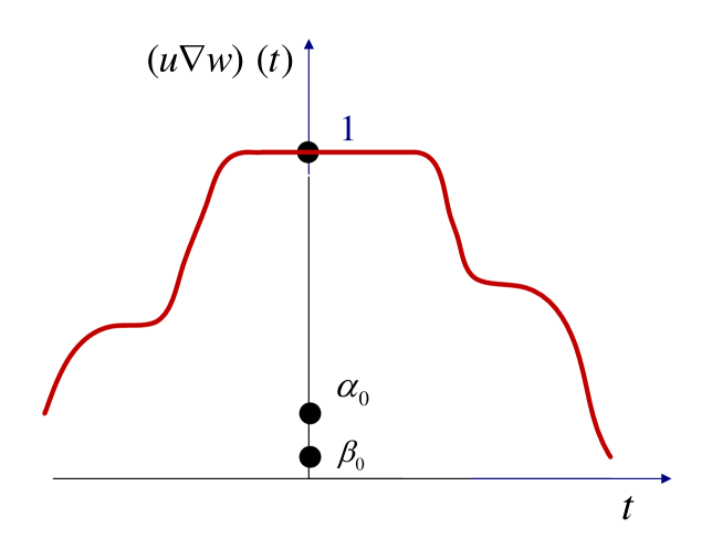
(a) $0<\alpha_{0}<1$, $0<\beta_{0}<1$

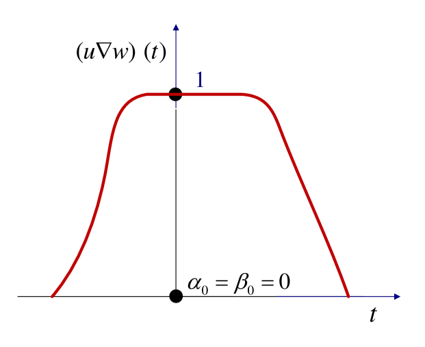
(b) $\alpha_{0}=\beta_{0}=0$

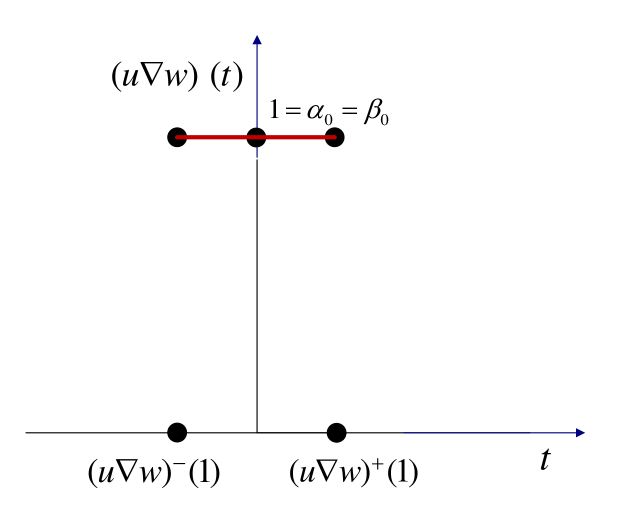
(c) $\alpha_{0}=\beta_{0}=1$

Figure 1: Some examples of $u\nabla w$

Since $w$ satisfies condition (i), from Theorem 3.13, we know that $u\nabla w\in\mathcal{F}_{\mathrm{C}}(\mathbb{R})$. To show $u\nabla w\in\mathcal{F}_{\mathrm{D}}(\mathbb{R})$ is equivalent to prove that $u\nabla w$ is differentiable at each inner point of $[u\nabla w]_{0}$.

Let $x$ be an inner point of $[u\nabla w]_{0}$, i.e. $x\in((u\nabla w)^{-}(\alpha_{0}),(u\nabla w)^{+}(\beta_{0}))$. From statement A10, we know that $(u\nabla w)^{\prime}(x)=0$ when $(u\nabla w)(x)=1$. By statement A9, we obtain that $(u\nabla w)^{\prime}(x)=0$ when $x$ is neither an endpoint of an $\alpha$-cut nor an endpoint of a strong-$\alpha$-cut.

Next, we consider the rest situation of $x$, i.e. $(u\nabla w)(x)<1$ and $x$ is an endpoint of an $\alpha$-cut or an endpoint of a strong-$\alpha$-cut. We split this situation into two cases. It is clear that $\alpha<1$ in these two cases.

Case (A) $x=(u\nabla w)^{-}(\alpha)$ ($(u\nabla w)_{s}^{-}(\alpha)$, $(u\nabla w)^{+}(\alpha)$, $(u\nabla w)_{s}^{+}(\alpha)$) with $(u\nabla w)(x)<1$, and both $u^{-}(\alpha)$ and $w^{-}(\alpha)$ ($u_{s}^{-}(\alpha)$ and $w_{s}^{-}(\alpha)$, $u^{+}(\alpha)$ and $w^{+}(\alpha)$, $u_{s}^{+}(\alpha)$ and $w_{s}^{+}(\alpha)$) being inner points of $[u]_{0}$ and $[w]_{0}$, respectively.

Note that $u\in\mathcal{F}_{\mathrm{N}}(\mathbb{R})\cap\mathcal{F}_{\mathrm{C}}(\mathbb{R})$ and $w\in\mathcal{F}_{\mathrm{D}}(\mathbb{R})$, hence $w$ is differentiable at each inner point and $u$ is differentiable at each inner point $y$ when $u(y)<1$. So, by statements A1–A8, we can compute $(u\nabla w)^{\prime}(x)$. For example, suppose that $x=(u\nabla w)^{-}(\alpha)=u^{-}(\alpha)+w^{-}(\alpha)$, and both $u^{-}(\alpha)$ and $w^{-}(\alpha)$ are inner points of $[u]_{0}$ and $[w]_{0}$, then, by statements A1 and A2, we obtain the differentiability of $u\nabla w$ at $x$.

Case (B) $x=(u\nabla w)^{-}(\alpha)$ ($(u\nabla w)_{s}^{-}(\alpha)$, $(u\nabla w)^{+}(\alpha)$, $(u\nabla w)_{s}^{+}(\alpha)$) with $(u\nabla w)(x)<1$ and $x$ is not in Case (A).

We claim that the following situations will not occur.

i

$x=(u\nabla w)_{s}^{-}(\alpha)$, $u_{s}^{-}(\alpha)=u^{-}(0)$ and $w_{s}^{-}(\alpha)=w^{-}(0)$.

ii

$x=(u\nabla w)_{s}^{+}(\alpha)$, $u_{s}^{+}(\alpha)=u^{+}(0)$ and $w_{s}^{+}(\alpha)=w^{+}(0)$.

iii

$w^{-}(0)<w_{s}^{-}(\alpha)=w^{+}(0)$.

iv

$w^{-}(0)=w_{s}^{+}(\alpha)<w^{+}(0)$.

In fact, if $x=(u\nabla w)_{s}^{-}(\alpha)$, $u_{s}^{-}(\alpha)=u^{-}(0)$ and $w_{s}^{-}(\alpha)=w^{-}(0)$, then $x=(u\nabla w)_{s}^{-}(\alpha)=u^{-}(0)+w^{-}(0)=(u\nabla w)^{-}(0)$ is not an inner point of $[u\nabla w]_{0}$. Hence situation (i) can not occur. Similarly, situation (ii) does not occur. Since $w\in\mathcal{F}_{\mathrm{C}}(\mathbb{R})$, by Lemma 5.4, we know that situations (iii) and (iv) will not occur.

If $x=(u\nabla w)^{-}(\alpha)$ is an inner point of $[u\nabla w]_{0}$, we obtain $1>\alpha>\alpha_{0}$. Note that $w$ is in $\mathcal{F}_{\mathrm{D}}(\mathbb{R})$, hence $w^{-}(\alpha_{0})<w^{-}(\alpha)<w^{-}(1)$, and therefore $u^{-}(\alpha_{0})<u^{-}(\alpha)=u^{+}(0)$. So case (B) can be divided into the following subcases.

Bi

$x=(u\nabla w)_{s}^{-}(\alpha)$ and $u_{s}^{-}(\alpha)=u^{-}(0)$.

Bii

$x=(u\nabla w)_{s}^{+}(\alpha)$ and $u_{s}^{+}(\alpha)=u^{+}(0)$.

Biii

$x=(u\nabla w)_{s}^{-}(\alpha)$, $w_{s}^{-}(\alpha)=w^{-}(0)$ and $u^{-}(0)<u_{s}^{-}(\alpha)<u^{+}(0)$.

Biv

$x=(u\nabla w)_{s}^{+}(\alpha)$, $w_{s}^{+}(\alpha)=w^{+}(0)$ and $u^{-}(0)<u_{s}^{+}(\alpha)<u^{+}(0)$.

Bv

$x=(u\nabla w)_{s}^{-}(\alpha)$, $w_{s}^{-}(\alpha)=w^{-}(0)$ and $u^{-}(0)<u_{s}^{-}(\alpha)=u^{+}(0)$.

Bvi

$x=(u\nabla w)_{s}^{+}(\alpha)$, $w_{s}^{+}(\alpha)=w^{+}(0)$ and $u^{-}(0)=u_{s}^{+}(\alpha)<u^{+}(0)$.

Bvii

$x=(u\nabla w)_{s}^{-}(\alpha)$, $w^{-}(0)<w_{s}^{-}(\alpha)<w^{+}(0)$ and $u^{-}(0)<u_{s}^{-}(\alpha)=u^{+}(0)$.

Bviii

$x=(u\nabla w)_{s}^{+}(\alpha)$, $w^{-}(0)<w_{s}^{+}(\alpha)<w^{+}(0)$ and $u^{-}(0)=u_{s}^{+}(\alpha)<u^{+}(0)$.

Bix

$x=(u\nabla w)^{-}(\alpha)$, $w^{-}(0)<w^{-}(\alpha)<w^{-}(1)$ and $u^{-}(0)<u^{-}(\alpha)=u^{+}(0)$.

Bx

$x=(u\nabla w)^{+}(\alpha)$, $w^{+}(1)<w^{+}(\alpha)<w^{+}(0)$ and $u^{-}(0)=u^{+}(\alpha)<u^{+}(0)$.

Since $u\in\mathcal{F}_{\mathrm{C}}(\mathbb{R})$, by Lemma 5.4, we know that subcases Bv–Bx do not occur, i.e., case (B) can be decomposed into four subcases: Bi–Biv. Notice that if $u\in\mathcal{F}_{\mathrm{N}}(\mathbb{R})$, then $w$ satisfies condition (iii). So, by statements B1–B4, we can prove the differentiability of $u\nabla w$ at $x$. $\quad\Box$

Now we give some examples to illustrate Theorem 5.7. By Example 5.8, we describe the role of condition (i) in Theorem 5.7.

Example 5.8

(a) $u$

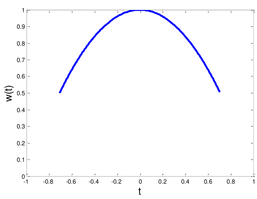
(b) $w$

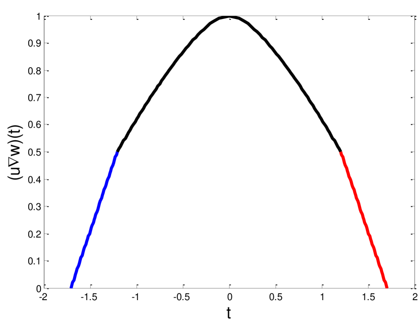
(c) $u\nabla w$

Figure 2: Fuzzy numbers in Example 5.8

Suppose

$$u(t)=\left\{\begin{array}[]{ll}t+1,&t\in[-1,0],\\ 1-t,&t\in[0,1],\\ 0,&t\notin[-1,1].\end{array}\right.$$

Observe that $u$ is differentiable on $(-1,1)\setminus\{0\}$. We can see that $u\in\mathcal{F}_{\mathrm{N}}(\mathbb{R})\cap\mathcal{F}_{\mathrm{C}}(\mathbb{R})$ and

$$[u]_{\alpha}=[-1+\alpha,\ 1-\alpha]$$

for all $\alpha\in[0,1]$. See Fig. 2a for the figure of $u$. Let

$$w(t)=\left\{\begin{array}[]{ll}1-t^{2},&t\in[-\sqrt{0.5},\sqrt{0.5}],\\ 0,&t\notin[-\sqrt{0.5},\sqrt{0.5}],\end{array}\right.$$

then

$$[w]_{\alpha}=\left\{\begin{array}[]{ll}[-\sqrt{1-\alpha},\sqrt{1-\alpha}],&\alpha\in[0.5,1],\\ \mbox{}[-\sqrt{0.5},\sqrt{0.5}],&\alpha\notin[0,0.5].\end{array}\right.$$

See Fig. 2b for the figure of $w$. It can be checked that $w$ is differentiable on $(-0.5,0.5)$, i.e. $w\in\mathcal{F}_{\mathrm{D}}(\mathbb{R})$. Notice that

$$w^{\prime}(w^{-}(1))=w^{\prime}(w^{+}(1))=w^{\prime}(0)=0,$$

$$w(w^{-}(0))=0.5\not=0=u(u^{-}(0),$$

$$w(w^{+}(0))=0.5\not=0=u(u^{+}(0)),$$

thus we know that $u$ and $w$ satisfy all but condition (i) in Theorem 5.7. We will see that $w$ is not a smoother of $u$. In fact, it can be computed that

$$[u\nabla w]_{\alpha}=[u]_{\alpha}+[w]_{\alpha}=\left\{\begin{array}[]{ll}[-1+\alpha-\sqrt{1-\alpha},\ 1-\alpha+\sqrt{1-\alpha}],&\alpha\in[0.5,1],\\ \mbox{}[-1+\alpha-\sqrt{0.5},\ 1-\alpha+\sqrt{0.5}],&\alpha\notin[0,0.5].\end{array}\right.$$

Now we can plot the figure of $u\nabla w$ in Fig 2c, and obtain

$$(u\nabla w)(t)=\left\{\begin{array}[]{ll}1+t+\sqrt{0.5},&t\in[-1-\sqrt{0.5},-0.5-\sqrt{0.5}],\\ t+0.5\sqrt{1-4t}+0.5,&t\in[-0.5-\sqrt{0.5},0],\\ -t+0.5\sqrt{1+4t}+0.5,&t\in[0,0.5+\sqrt{0.5}],\\ 1-t+\sqrt{0.5},&t\in[0.5+\sqrt{0.5},1+\sqrt{0.5}].\end{array}\right.$$

It is easy to check that $u\nabla w$ is not differentiable at $t=-0.5-\sqrt{0.5}$ and $t=0.5+\sqrt{0.5}$, and therefore $u\nabla w\notin\mathcal{F}_{\mathrm{D}}(\mathbb{R})$. So $w$ is not a smoother of $u$. This means that condition (i) in Theorem 5.7 can not be omitted.

In Proposition 2.3, it pointed out that if $u\in\mathcal{F}_{\mathrm{T}}(\mathbb{R})$, then $u\nabla w_{p}\in\mathcal{F}_{\mathrm{D}}(\mathbb{R})$. This means that $w_{p}$, $p>0$, can serve as smoothers for all fuzzy numbers in $\mathcal{F}_{\mathrm{T}}(\mathbb{R})$. In Theorem 5.7, it finds that $w_{p}$, $p>0$, can also work as smoothers even for fuzzy numbers not in $\mathcal{F}_{\mathrm{T}}(\mathbb{R})$. The following example is given to show this fact.

Example 5.9

Suppose

$$u(t)=\left\{\begin{array}[]{ll}-0.5(t^{2}+2t),&\ t\in[-2,-1),\\ 0.5,&\ t\in[-1,-0.5],\\ 2t^{2}+2t+1,&\ t\in(-0.5,0],\\ 2t^{2}-2t+1,&\ t\in(0,0.5),\\ 0.5,&\ t\in[0.5,1],\\ -0.5(t^{2}-2t),&\ t\in(1,2],\\ 0,&\ t\not\in[-2,2].\end{array}\right.$$

See Fig. 3a for the figure of $u$.

(a) $u$

(b) $w_{1}$

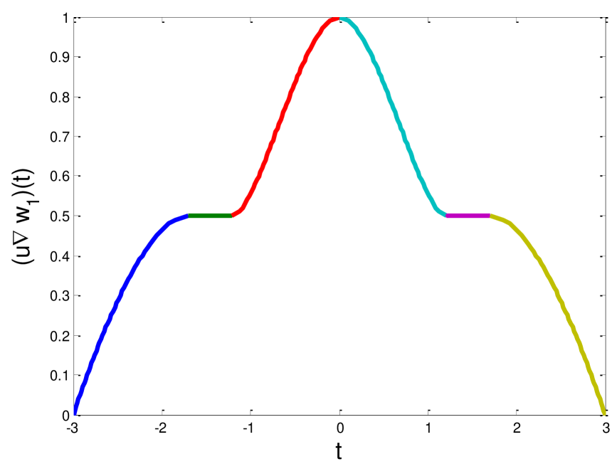
(c) $u\nabla w_{1}$

Figure 3: Fuzzy numbers $u$, $w_{1}$ and $u\nabla w_{1}$ in Example 5.9

Clearly $u$ is not strictly increasing on $[-1,-0.5]$ and is not strictly decreasing on $[0.5,1]$. Therefore $u$ is in $\mathcal{F}_{\mathrm{N}}(\mathbb{R})\cap\mathcal{F}_{\mathrm{C}}(\mathbb{R})$ but not in $\mathcal{F}_{\mathrm{T}}(\mathbb{R})$. Take $w_{1}$ defined in (2), i.e.

$$w_{1}(t)=\left\{\begin{array}[]{ll}1-t^{2},&\ t\in[-1,1],\\ 0,&\ t\notin[-1,1].\end{array}\right.$$

The figure of $w_{1}$ is in Fig 3b. It is easy to check that $u$ and $w_{1}$ satisfy all the conditions in Theorem 5.7. Thus $w_{1}$ is a smoother for $u$. Now, we validate this assertion by computing $u\nabla w_{1}$. Note that

$$[u \nabla w_{1}]_{\alpha}=[u]_{\alpha}+[w_{1}]_{\alpha}$$

$$=\left\{\begin{array}[]{ll}[-\sqrt{1-2\alpha}-1-\sqrt{1-\alpha},\ 1+\sqrt{1-2\alpha}+\sqrt{1-\alpha}\,],&\ \alpha\in[0,0.5],\\ \mbox{}[0.5(-1+\sqrt{2\alpha-1})-\sqrt{1-\alpha},\ 0.5(1-\sqrt{2\alpha-1})+\sqrt{1-\alpha}],&\ \alpha\in(0.5,1],\end{array}\right.$$

and thus we can obtain that

$$(u\nabla w_{1})(t)$$

$$= \left\{\begin{array}[]{ll}-(t+1)(3t+2(2t^{2}+4t+3)^{0.5}+3),&t\in[-3,-1-\sqrt{0.5}],\\ 0.5,&t\in(-1-\sqrt{0.5},-0.5-\sqrt{0.5}],\\ (4t(1-2t-2t^{2})^{0.5})/9-(2t)/9+(2(1-2t-2t^{2})^{0.5})/9-(2t^{2})/9+7/9,\\ &t\in(-0.5-\sqrt{0.5},0],\\ (-4t(1+2t-2t^{2})^{0.5})/9+(2t)/9+(2(1+2t-2t^{2})^{0.5})/9-(2t^{2})/9+7/9,\\ &t\in[0,0.5+\sqrt{0.5}),\\ 0.5,&t\in[0.5+\sqrt{0.5},1+\sqrt{0.5}),\\ (t-1)(-3t+2(2t^{2}-4t+3)^{0.5}+3),&t\in[1+\sqrt{0.5},3],\\ 0,&t\not\in[-3,3].\end{array}\right.$$

The figure of $u\nabla w_{1}$ is in Fig 3c. It can be computed that

$$(u\nabla w_{1})^{\prime}(-1-\sqrt{0.5})=(u\nabla w_{1})^{\prime}(-0.5-\sqrt{0.5})=0,$$

$$(u\nabla w_{1})^{\prime}(0)=0,$$

$$(u\nabla w_{1})^{\prime}(1+\sqrt{0.5})=(u\nabla w_{1})^{\prime}(0.5+\sqrt{0.5})=0.$$

Combined with the expression of $u\nabla w_{1}$, it now follows that $u\nabla w_{1}$ is differentiable on $(-3,3)$, i.e., $u\nabla w_{1}\in\mathcal{F}_{\mathrm{D}}(\mathbb{R})$. This means that $w_{1}$ can work as a smoother for the fuzzy number $u$ which is in $(\mathcal{F}_{\mathrm{N}}(\mathbb{R})\cap\mathcal{F}_{\mathrm{C}}(\mathbb{R}))\backslash\mathcal{F}_{\mathrm{T}}(\mathbb{R})$.

However $w_{p}$, $p>0$, may not be smoothers for a fuzzy number $u$ which is not in $\mathcal{F}_{\mathrm{C}}(\mathbb{R})$. The following example is given to show this fact.

Example 5.10

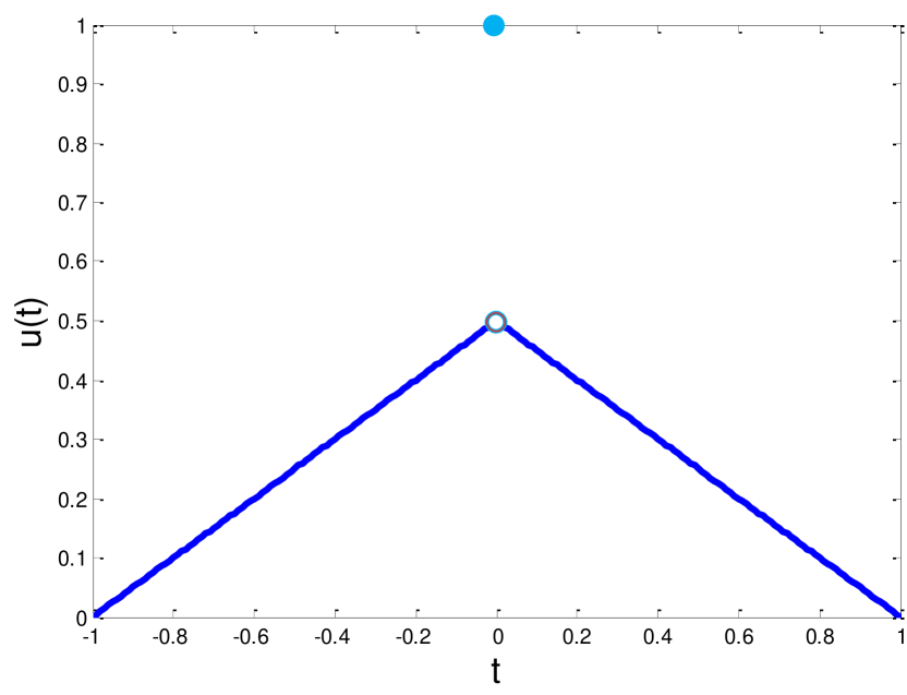
(a) $u$

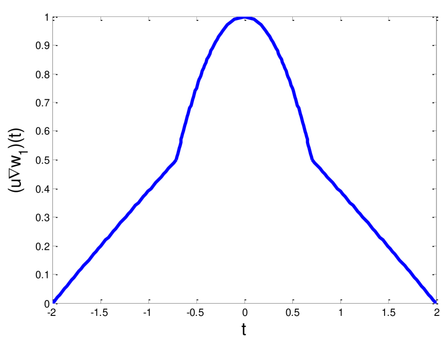
(b) $u\nabla w_{1}$

Figure 4: Fuzzy numbers in Example 5.10

Suppose that

$$u(t)=\left\{\begin{array}[]{ll}0.5t+0.5,&\ t\in[-1,0),\\ -0.5t+0.5,&\ t\in(0,1],\\ 1,&\ t=0,\\ 0,&\ t\notin[-1,1].\end{array}\right.$$

See Fig. 4a for the figure of $u$. It is easy to check that $u\in(\mathcal{F}_{\mathrm{T}}(\mathbb{R})\cap\mathcal{F}_{\mathrm{N}}(\mathbb{R}))\backslash\mathcal{F}_{\mathrm{C}}(\mathbb{R})$. But

$$(u\nabla w_{1})(t)=\left\{\begin{array}[]{ll}0.125(-8t+9)^{0.5}+0.5t+0.375,&\ t\in[-2,-\sqrt{0.5}],\\ 1-t^{2},&\ t\in[-\sqrt{0.5},\sqrt{0.5}],\\ 0.125(8t+9)^{0.5}-0.5t+0.375,&\ t\in[\sqrt{0.5},2].\end{array}\right.$$

See Fig. 4b for the figure of $u\nabla w_{1}$. It is easy to check that $u\nabla w_{1}$ is not differentiable at $t=\pm\sqrt{0.5}$. Thus $u\nabla w_{1}\notin\mathcal{F}_{\mathrm{D}}(\mathbb{R})$. So $w_{1}$ is not a smoother for $u$. This means that $w_{p}$, $p>0$, may not work as smoothers for fuzzy numbers in $\mathcal{F}_{\mathrm{T}}(\mathbb{R})\cap\mathcal{F}_{\mathrm{N}}(\mathbb{R})$ but not in $\mathcal{F}_{\mathrm{C}}(\mathbb{R})$.

Remark 5.11

Define

$$\mathcal{F}^{0}_{\mathrm{NC}}(\mathbb{R})=\{u\in\mathcal{F}_{\mathrm{N}}(\mathbb{R})\cap\mathcal{F}_{\mathrm{C}}(\mathbb{R}):u(u^{-}(0))=u(u^{+}(0))=0\}.$$

Let $u$ be a fuzzy number in $\mathcal{F}^{0}_{\mathrm{NC}}(\mathbb{R})$. Suppose that $Z_{p}^{f}$ is a fuzzy number defined by (3) and satisfies the conditions in Proposition 2.4, i.e. $p>0$ and $f:[0,1]\to[0,1]$ is a differentiable and strictly decreasing function with $f(0)=1$, $f(1)=0$, and $\lim_{\alpha\to 1-}f^{\prime}(\alpha)=-\infty$. Then $u$ and $Z_{p}^{f}$ satisfy all conditions in Theorem 5.7. So, by Theorem 5.7, we know that $Z_{p}^{f}$ presented in Proposition 2.4 are smoothers for fuzzy numbers in $\mathcal{F}^{0}_{\mathrm{NC}}(\mathbb{R})$. Let $f=\sqrt{1-t}$, then $Z_{p}^{f}$ is just $w_{p}$ defined in (2). So $w_{p}$, $p>0$, are also smoothers for fuzzy numbers in $\mathcal{F}^{0}_{\mathrm{NC}}(\mathbb{R})$.

Theorem 5.7 shows that how to choose smoothers for fuzzy numbers in $\mathcal{F}_{\mathrm{N}}(\mathbb{R})\cap\mathcal{F}_{\mathrm{C}}(\mathbb{R})$. Now we discuss how to use this method to construct a sequence of smooth fuzzy numbers to approximate the original fuzzy number.

Suppose that $u_{l,r}$ is a fuzzy number in $\mathcal{F}_{\mathrm{N}}(\mathbb{R})\cap\mathcal{F}_{\mathrm{C}}(\mathbb{R})$ with $u(u^{-}(0))=l$ and $u(u^{+}(0))=r$. Define corresponding $v_{l,r,p}$, $p>0$, as follows.

$$v_{l,r,p}(t)=\left\{\begin{array}[]{ll}1-{\left(t/p\right)}^{2},&\ t\in[-p\sqrt{1-l},p\sqrt{1-r}],\\ 0,&\ t\notin[-p\sqrt{1-l},\ p\sqrt{1-r}].\end{array}\right.$$

It is easy to check that $v_{l,r,p}(v_{l,r,p}^{-}(0))=l$, $v_{l,r,p}(v_{l,r,p}^{+}(0))=r$, and then we can see that, for each $p>0$, $u_{l,r}$ and $v_{l,r,p}$ satisfy all the conditions in Theorem 5.7. So $v_{l,r,p}$, $p>0$, are smoothers for $u_{l,r}$. In the following, for simplicity, we use $u$ and $v_{p}$ to denote $u_{l,r}$ and $v_{l,r,p}$, respectively. It is easy to observe that if $l=r=0$, then $v_{p}$ is just $w_{p}$ defined in (2).

Notice that $d_{\infty}(u\nabla v_{p},\ u)\leq\max\{p\sqrt{1-l},\ p\sqrt{1-t}\}\leq p$ and $u\nabla v_{p}\in\mathcal{F}_{\mathrm{D}}(\mathbb{R})$, thus we have the following conclusion.

Theorem 5.12

Given $u$ in $\mathcal{F}_{\mathrm{N}}(\mathbb{R})\cap\mathcal{F}_{\mathrm{C}}(\mathbb{R})$, then

$$d_{\infty}(u\nabla v_{1/n},\ u)\leq 1/n.$$

So the smooth fuzzy numbers sequence $\{u\nabla v_{1/n}:\ n\in\mathbb{N}\}$ approximates $u$ according to the supremum metric $d_{\infty}$.

The above theorem shows that, for each fuzzy number $u\in\mathcal{F}_{\mathrm{N}}(\mathbb{R})\cap\mathcal{F}_{\mathrm{C}}(\mathbb{R})$, we can find a sequence of smooth fuzzy numbers $\{u\nabla v_{1/n}\}$ which approximates $u$ in $d_{\infty}$ metric. By Theorem 5.7, we can construct other types of smoothers for $u_{l,r}$. For example, define fuzzy numbers $\xi_{l,r,p}^{f,g}$ as follows:

$$\xi_{l,r,p}^{f,g}(t)=\left\{\begin{array}[]{ll}f(\frac{t-pa}{pb-pa}),&\ t\in[pa,pb],\\ 1,&\ t\in[pb,pc],\\ g(\frac{t-pc}{pd-pc}),&\ t\in[pc,pd],\\ 0,&\ t\notin[pa,pd],\end{array}\right.$$

where $a<b<c<d$, $p>0$, $f:[0,1]\to[l,1]$ is an increasing and differentiable function which satisfies that $f(0)=l$, $f(1)=1$, and $f_{-}^{\prime}(1)=0$, and $g:[0,1]\to[r,1]$ is a decreasing and differentiable function which satisfies that $g(0)=1$, $g(1)=r$, and $g_{+}^{\prime}(0)=0$. Then it can be checked that $\xi_{l,r,p}^{f,g}$, $p>0$, are smoothers of $u_{l,r}$ and that $u_{l,r}\nabla\xi_{l,r,p}^{f,g}$ converges to $u_{l,r}$ as $p\to 0$.

Next we consider how to use the convolution method to construct a smooth approximation for an arbitrary fuzzy number $u$ in $\mathcal{F}_{\mathrm{C}}(\mathbb{R})$. The following lemmas are needed.

Lemma 5.13

Suppose that $w\in\mathcal{F}_{\mathrm{D}}(\mathbb{R})$ and that $\alpha\in[0,1]$, then
(i)  $w^{\prime}(w^{-}(\alpha))=0$ is equivalent to $w^{\prime}(w_{s}^{-}(\alpha))=0$;
(ii)  $w^{\prime}(w^{+}(\alpha))=0$ is equivalent to $w^{\prime}(w_{s}^{+}(\alpha))=0$.

Proof   (i)   If $w^{-}(\alpha)=w_{s}^{-}(\alpha)$, then obviously $w^{\prime}(w^{-}(\alpha))=0$ is equivalent to $w^{\prime}(w_{s}^{-}(\alpha))=0$. If $w^{-}(\alpha))<w_{s}^{-}(\alpha)$, it then follows from $w\in\mathcal{F}_{\mathrm{D}}(\mathbb{R})$ that $w^{\prime}(w^{-}(\alpha))=w^{\prime}(w_{s}^{-}(\alpha))=0$.

(ii)  The desired conclusion can be proved similarly as (i). $\quad\Box$

Lemma 5.14

Let $u\in\mathcal{F}(\mathbb{R})$. Suppose that $w\in\mathcal{F}_{\mathrm{D}}(\mathbb{R})$ satisfies condition (i) and the following condition (iv):
(iv)  Suppose that $x\in(u^{-}(0),u^{+}(0))$ is a non-differentiable point of $u$, then
(iv-1)  if $u^{-}(0)<x<u^{-}(1)$, then $w_{+}^{\prime}(w^{-}(\alpha))=0$, where $\alpha:=u(x)$;
(iv-2)  if $u^{+}(1)<x<u^{+}(0)$, then $w_{-}^{\prime}(w^{+}(\beta))=0$, where $\beta:=u(x)$.
Then, for each $z\in((u\nabla w)^{-}(0),(u\nabla w)^{+}(0))$ with $(u\nabla w)(z)<1$,

C1

$(u\nabla w)^{\prime}(z)=0$ when $z=(u\nabla w)^{-}(\alpha)$ and $u^{-}(\alpha)\in(u^{-}(0),u^{+}(0))$ is a continuous and non-differentiable point of $u$.

C2

$(u\nabla w)^{\prime}(z)=0$ when $z=(u\nabla w)_{s}^{-}(\alpha)$ and $u_{s}^{-}(\alpha)\in(u^{-}(0),u^{+}(0))$ is a continuous and non-differentiable point of $u$.

C3

$(u\nabla w)^{\prime}(z)=0$ when $z=(u\nabla w)^{+}(\alpha)$ and $u^{+}(\alpha)\in(u^{-}(0),u^{+}(0))$ is a continuous and non-differentiable point of $u$.

C4

$(u\nabla w)^{\prime}(z)=0$ when $z=(u\nabla w)_{s}^{+}(\alpha)$ and $u_{s}^{+}(\alpha)\in(u^{-}(0),u^{+}(0))$ is a continuous and non-differentiable point of $u$.

Proof  We only prove statements C1 and C2. Other statements can be proved similarly. Set $\alpha_{0}:=u(u^{-}(0))=w(w^{-}(0))=(u\nabla w)((u\nabla w)^{-}(0))$.

Suppose that $z=(u\nabla w)^{-}(\alpha)$ and that $u^{-}(\alpha)\in(u^{-}(0),u^{+}(0))$ is a continuous and non-differentiable point of $u$. Then $\alpha_{0}<\alpha<1$, and hence $w^{-}(\alpha)\in(w^{-}(0),w^{+}(0))$. By Proposition 3.3, $u(u^{-}(\alpha))=\alpha$, and therefore, by condition (iv-1), $w^{\prime}(w^{-}(\alpha))=0$. It thus follows from Theorem 4.1 (i), (ii) that $(u\nabla w)^{\prime}(z)=(u\nabla w)^{\prime}((u\nabla w)^{-}(\alpha))=0$. So statement C1 is true.

Suppose that $z=(u\nabla w)_{s}^{-}(\alpha)$ and $u_{s}^{-}(\alpha)\in(u^{-}(0),u^{+}(0))$ is a continuous and non-differentiable point of $u$. Then, by Proposition 3.3, $u(u_{s}^{-}(\alpha))=\alpha<1$, and hence, by condition (iv-1), $w_{+}^{\prime}(w^{-}(\alpha))=0$. If $\alpha>\alpha_{0}$, then both $w^{-}(\alpha)$ and $w_{s}^{-}(\alpha)$ are inner points. Thus by Lemma 5.13 $w^{\prime}(w_{s}^{-}(\alpha))=0$. So it follows from Theorem 4.1 (iii), (iv) that $(u\nabla w)^{\prime}(z)=(u\nabla w)^{\prime}((u\nabla w)_{s}^{-}(\alpha))=0$. If $\alpha=\alpha_{0}$. Note that $w^{-}(\alpha_{0})\leq w_{s}^{-}(\alpha_{0})$, we know that $w_{+}^{\prime}(w_{s}^{-}(\alpha_{0}))=0$, and hence $(u\nabla w)_{+}^{\prime}(z)=(u\nabla w)_{+}^{\prime}((u\nabla w)_{s}^{-}(\alpha_{0}))=0$. Since $z$ is an inner point of $[u\nabla w]_{0}$, we obtain that $(u\nabla w)^{\prime}(z)=0$. Thus statement C2 is proved. $\quad\Box$

The following theorem presents a method to find smoothers in $\mathcal{F}_{\mathrm{C}}(\mathbb{R})$. From Theorem 5.7, we have already given a way to pick smoothers for fuzzy numbers in $\mathcal{F}_{\mathrm{C}}(\mathbb{R})\cap\mathcal{F}_{\mathrm{N}}(\mathbb{R})$. Now our considerations need include fuzzy numbers in $\mathcal{F}_{\mathrm{C}}(\mathbb{R})\backslash\mathcal{F}_{\mathrm{N}}(\mathbb{R})$ which have one or more non-differentiable points in $[u]_{0}\backslash[u]_{1}$.

Theorem 5.15

Suppose that $u\in\mathcal{F}_{\mathrm{C}}(\mathbb{R})$ and that $w\in\mathcal{F}_{\mathrm{D}}(\mathbb{R})$, then $w$ is a smoother of $u$, i.e. $u\nabla w\in\mathcal{F}_{\mathrm{D}}(\mathbb{R})$, when $w$ satisfies the conditions (i), (ii), and (iv).

Proof  To prove that $u\nabla w\in\mathcal{F}_{\mathrm{D}}(\mathbb{R})$, we adopt the same procedure as in the proof of Theorem 5.7. The proof is divided into the same situations as the proof of Theorem 5.7. Since $u\in\mathcal{F}_{\mathrm{C}}(\mathbb{R})$, we know that each inner point of $[u]_{0}$ is a continuous point of $u$. Hence if $w$ satisfies condition (iv), then $w$ must satisfy condition (iii). Thus only case (A) need to be reconsidered.

Case (A) $x=(u\nabla w)^{-}(\alpha)$ ($(u\nabla w)_{s}^{-}(\alpha)$, $(u\nabla w)^{+}(\alpha)$ $(u\nabla w)_{s}^{+}(\alpha)$) with $(u\nabla w)(x)<1$, and both $u^{-}(\alpha)$ and $w^{-}(\alpha)$ ($u_{s}^{-}(\alpha)$ and $w_{s}^{-}(\alpha)$, $u^{+}(\alpha)$ and $w^{+}(\alpha)$, $u_{s}^{+}(\alpha)$ and $w_{s}^{+}(\alpha)$) being inner points of $[u]_{0}$ and $[w]_{0}$, respectively.

It is easy to see that $\alpha<1$. Note that $u\in\mathcal{F}_{\mathrm{C}}(\mathbb{R})$, this implies that each inner point of $[u]_{0}$ is a continuous point of $u$. If $u^{-}(\alpha)$ ($u_{s}^{-}(\alpha)$, $u^{+}(\alpha)$, $u_{s}^{+}(\alpha)$) is a continuous but non-differentiable point of $u$, then by statements C1–C4, we know that $(u\nabla w)^{\prime}(x)=0$. If $u^{-}(\alpha)$ ($u_{s}^{-}(\alpha)$, $u^{+}(\alpha)$, $u_{s}^{+}(\alpha)$) is a differentiable point of $u$, then by statements A1–A8, we can compute $(u\nabla w)^{\prime}(x)$. $\quad\Box$

The following is a concrete example by which we illustrate how to use the results in Theorem 5.15 to construct smoothers for fuzzy numbers in $\mathcal{F}_{\mathrm{C}}(\mathbb{R})$.

Example 5.16

Suppose

$$u(t)=\left\{\begin{array}[]{ll}0.5+t,&\ t\in[-0.5,0),\\ 0.5+0.5t,&\ t\in[0,1],\\ 2-t,&\ t\in(1,2],\\ 0,&\ t\not\in[-0.5,2].\end{array}\right.$$

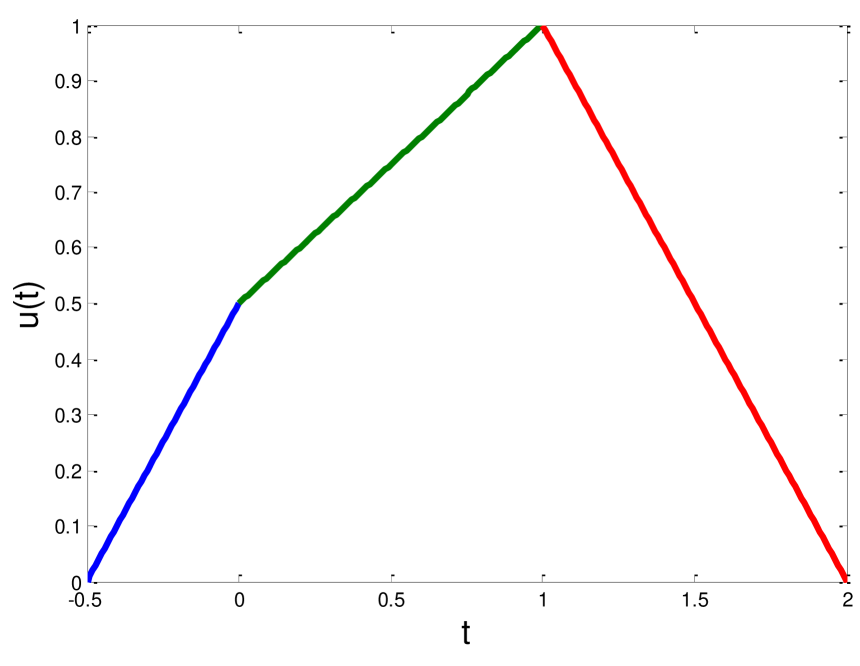
(a) $u$

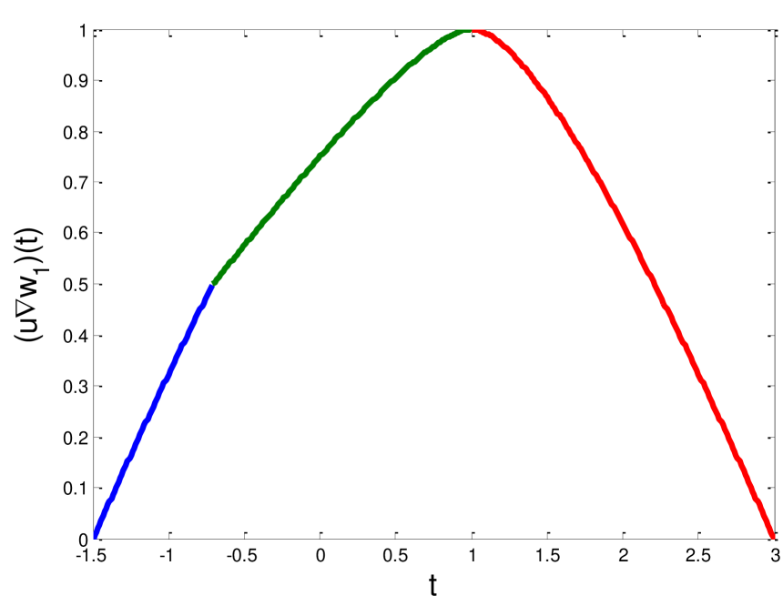
(b) $u\nabla w_{1}$

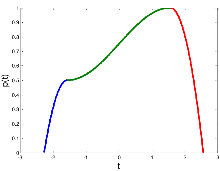
(c) $p$

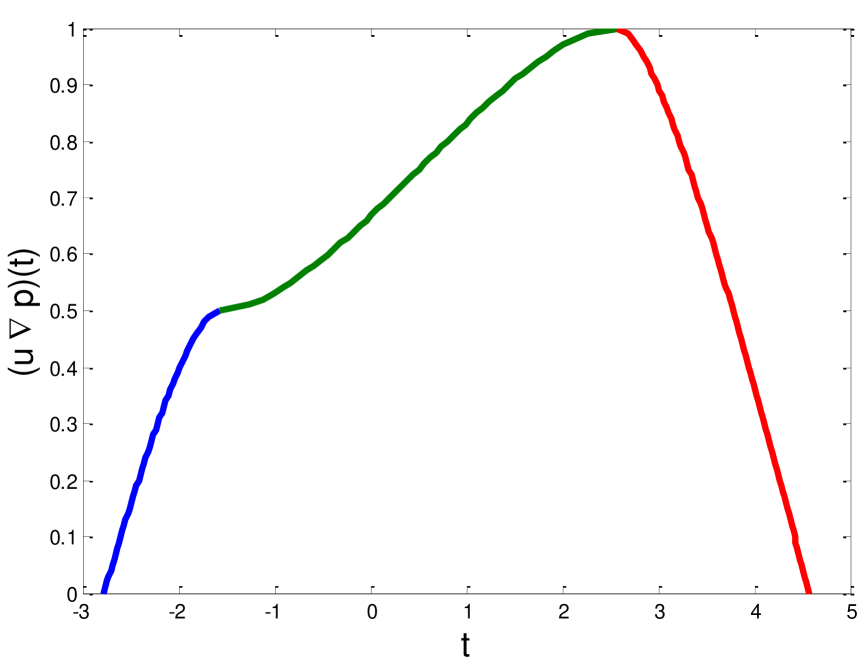
(d) $u\nabla p$

Figure 5: Fuzzy numbers in Example 5.16

Obviously, $u$ is in $\mathcal{F}_{\mathrm{C}}(\mathbb{R})$ and has a non-differentiable point $u^{-}(0.5)=0$. See Fig. 5a for the figure of $u$.

First let’s see whether $w_{1}$ defined in (2) can work as a smoother for $u$. Note that ${w_{1}}^{\prime}({w_{1}}^{-}(0.5))\not=0$, thus $u$ and $w_{1}$ do not satisfy the conditions in Theorem 5.15. It can be deduced that

$$(u\nabla w_{1})(t)=\left\{\begin{array}[]{ll}\sqrt{\frac{3}{4}-t}+t,&\ \ t\in[-\frac{3}{2},-\sqrt{0.5}],\\ \frac{\sqrt{9-8t}+3+4t}{8},&\ \ t\in(-\sqrt{0.5},1],\\ \frac{\sqrt{4t-3}-2t+3}{2},&\ \ t\in(1,3],\\ 0,&\ \ t\notin[-\frac{3}{2},3].\end{array}\right.$$

See Fig. 5b for the figure of $u\nabla w_{1}$. Notice that $(u\nabla w_{1})^{\prime}_{-}(-\sqrt{0.5})=2-\sqrt{2}$, and $(u\nabla w_{1})^{\prime}_{+}(-\sqrt{0.5})=\frac{3-2\sqrt{2}}{14},$ it then follows that $u\nabla w_{1}$ is not differentiable at $(u\nabla w_{1})^{-}(0.5)=-\sqrt{0.5}$, so $u\nabla w_{1}\notin\mathcal{F}_{\mathrm{D}}(\mathbb{R})$. This means that $w_{1}$ is not a smoother of $u$.

Now we use the conclusions in Theorem 5.15 to construct a smoother for $u$. Consider a fuzzy number $p$ defined by

$$p(t)=\left\{\begin{array}[]{ll}0.5-(t+\pi/2)^{2},&\ t\in[-\pi/2-\sqrt{0.5},-\pi/2],\\ 0.25\sin t+0.75,&\ t\in[-\pi/2,\pi/2],\\ 1-(t-\pi/2)^{2},&\ t\in[\pi/2,1+\pi/2].\end{array}\right.$$

Then $p^{\prime}(p^{-}(0.5))=0$. See Fig. 5c for the figure of $p$. It’s easy to check that $u$ and $p$ satisfies all the conditions of Theorem 5.15. Thus by Theorem 5.15, $p$ is a smoother of $u$. To validate this assertion, we compute that

$$[u\nabla p]_{\alpha}=\left\{\begin{array}[]{ll}[-0.5\pi-(0.5-\alpha)^{0.5}+\alpha-0.5,\ 0.5\pi+(1-\alpha)^{0.5}+2-\alpha],&\ \alpha\in[0,0.5],\\ \mbox{}[\arcsin(4\alpha-3)+2\alpha-1,\ 0.5\pi+(1-\alpha)^{0.5}+2-\alpha],&\ \alpha\in[0.5,1].\end{array}\right.$$

Now we can plot $u\nabla p$ in Fig. 5d, and obtain

$$(u\nabla p)(t)=\left\{\begin{array}[]{ll}\pi/2+t+(1-4t-2\pi)^{0.5}/2,&\ t\in[-\pi/2-\sqrt{0.5}-0.5,-\pi/2],\\ f(t),&\ t\in[-0.5\pi,1+0.5\pi],\\ \pi/2-t+(4t-2\pi-3)^{0.5}/2+3/2,&\ t\in[1+0.5\pi,3+0.5\pi],\end{array}\right.$$ (6)

where $f(t)$ is the inverse function of $g(\alpha)=\arcsin(4\alpha-3)+2\alpha-1$ when $\alpha\in[0.5,1]$.

It can be checked that $u\nabla p\in\mathcal{F}_{\mathrm{D}}(\mathbb{R})$. In fact, from the expression of $u\nabla p$, we know that it only need to show that $u\nabla p$ is differentiable at $-0.5\pi$ and $1+0.5\pi$. Use implicit differentiation to take $f^{\prime}$ as follows:

$$f^{\prime}(t)=(2+\frac{4}{\sqrt{1-(4\alpha(t)-3)^{2}}})^{-1}.$$

Then we have that $(u\nabla p)_{-}^{\prime}(-0.5\pi)=\frac{d}{dt}(\pi/2+t+(1-4t-2\pi)^{0.5}/2)|_{t=-0.5\pi}=0$ and $(u\nabla p)_{+}^{\prime}(-0.5\pi)=f^{\prime}(-0.5\pi)=0,$ hence

$$(u\nabla p)^{\prime}(-0.5\pi)=0.$$ (7)

Similarly, it can be computed that

$$(u\nabla p)^{\prime}(1+0.5\pi)=0.$$ (8)

It now follows from (6),(7) and (8) that $u\nabla p$ is differentiable on $(-\pi/2-\sqrt{0.5}-0.5,\ 3+0.5\pi)$, i.e, $u\nabla p\in\mathcal{F}_{\mathrm{D}}(\mathbb{R})$. So $p$ is a smoother of $u$. From this example we can see how condition (iv) takes effect.

Look at the construction of $p$. To make $u$ and $p$ satisfy the condition (iv), i.e. to assure $p^{\prime}(p^{-}(0.5))=p^{\prime}(-\pi/2)=0$, we use a polynomial function and a sine function to construct $p$. Along this line, given a fuzzy number $u\in\mathcal{F}_{\mathrm{C}}(\mathbb{R})$ with finite non-differentiable points, we can use polynomial functions, sine functions and cosine functions to construct a fuzzy number $\eta\in\mathcal{F}_{\mathrm{D}}(\mathbb{R})$ such that $u$ and $\eta$ satisfy all conditions in Theorem 5.15. To construct a smooth fuzzy numbers sequence to approximate $u$, put $\eta_{p}:=p\cdot\eta$, i.e.

$$\eta_{p}(t):=(p\cdot\eta)(t)=\eta(t/p)=\left\{\begin{array}[]{ll}\eta(t/p),&\ t\in p[\eta]_{0},\\ 0,&\ t\notin p[\eta]_{0},\end{array}\right.$$ (9)

where $p>0$ is a real number. Clearly $\eta=\eta_{1}$. It can be checked that

$$\eta(\eta^{-}(0))=\eta_{p}({\eta_{p}}^{-}(0)),\ \eta(\eta^{+}(0))=\eta_{p}({\eta_{p}}^{+}(0)),$$ (10)

and

$${\eta_{p}}_{-}^{\prime}(t)=\eta_{-}^{\prime}(t/p)/p,$$

$${\eta_{p}}_{+}^{\prime}(t)=\eta_{+}^{\prime}(t/p)/p$$

for all $t\in\mathbb{R}$. Thus we know $\eta_{p}\in\mathcal{F}_{\mathrm{D}}(\mathbb{R})$,

$${\eta_{p}}_{-}^{\prime}({\eta_{p}}^{-}(1))=\eta^{\prime}_{-}(\eta^{-}(1))/p,$$ (11)

$${\eta_{p}}_{+}^{\prime}({\eta_{p}}^{+}(1))=\eta^{\prime}_{+}(\eta^{+}(1))/p,$$ (12)

and

$$\eta_{p}^{\prime}({\eta_{p}}^{-}(\alpha))=\eta_{p}^{\prime}(p\cdot\eta^{-}(\alpha))=\eta^{\prime}(\eta^{-}(\alpha))/p,$$ (13)

$$\eta_{p}^{\prime}({\eta_{p}}^{+}(\alpha))=\eta_{p}^{\prime}(p\cdot\eta^{+}(\alpha))=\eta^{\prime}(\eta^{+}(\alpha))/p$$ (14)

for each $\alpha\in(0,1)$.

From eqs. (10)–(14), we know that $u$ and $\eta$ satisfy all the conditions in Theorem 5.15 is equivalent to that $u$ and $\eta_{p}$, $p>0$, satisfy all the conditions in Theorem 5.15. So we have the following conclusion.

Theorem 5.17

Given $u$ in $\mathcal{F}_{\mathrm{C}}(\mathbb{R})$. If the number of non-differentiable points of $u$ is finite, then there exists smoothers for $u$. Moreover, if $\eta$ is a smoother of $u$, then $p\cdot\eta$, $p>0$, are also smoothers of $u$, and

$$d_{\infty}(u,u\nabla(p\cdot\eta))\leq p\cdot\max\{|\eta^{+}(0)|,|\eta^{-}(0)|\}.$$

So $\{u\nabla(p\cdot\eta)\}$ converges to $u$ according to the supremum metric $d_{\infty}$ as $p\to 0$.

Finally, we consider how to smooth an arbitrarily given fuzzy number $u$, which may have non-continuous points in $(u^{-}(0),u^{+}(0))$.

Lemma 5.18

Suppose that $u\in\mathcal{F}(\mathbb{R})$ and that $w\in\mathcal{F}_{\mathrm{D}}(\mathbb{R})$ satisfies condition (i) and condition (v) listed below:

(v-1)

if $u^{-}(0)<x\leq u^{-}(1)$ and $u$ is not left-continuous at $x$, then $w_{+}^{\prime}(w^{-}(\beta))=0$, where $\beta=\lim_{y\to x-}u(y)$;

(v-2)

if $u^{+}(1)\leq x<u^{+}(0)$ and $u$ is not right-continuous at $x$, then $w_{-}^{\prime}(w^{+}(\gamma))=0$, where $\gamma=\lim_{y\to x+}u(y)$.

Then, given $x\in((u\nabla w)^{-}(0),(u\nabla w)^{+}(0))$ with $(u\nabla w)(x)<1$, the following statements hold.

B5

$(u\nabla w)^{\prime}(x)=0$ and $x=(u\nabla w)_{s}^{-}(0)$ when $x=(u\nabla w)_{s}^{-}(\alpha)$, $w_{s}^{-}(\alpha)=w^{-}(0)$ and $u^{-}(0)<u_{s}^{-}(\alpha)=u^{+}(0)$.

B6

$(u\nabla w)^{\prime}(x)=0$ and $x=(u\nabla w)_{s}^{+}(0)$ when $x=(u\nabla w)_{s}^{+}(\alpha)$, $w_{s}^{+}(\alpha)=w^{+}(0)$ and $u^{-}(0)=u_{s}^{+}(\alpha)<u^{+}(0)$.

Proof   We only prove statement B5. Statement B6 can be proved similarly. Set $w(w^{-}(0))=u(u^{-}(0))=(u\nabla w)((u\nabla w)^{-}(0)):=\alpha_{0}$. From $w_{s}^{-}(\alpha)=w^{-}(0)$ and $u^{-}(0)<u_{s}^{-}(\alpha_{0})=u^{+}(0)$, we know $\alpha=\alpha_{0}<1$ and $u^{-}(0)=u^{-}(\alpha_{0})<u_{s}^{-}(\alpha_{0})=u^{-}(1)=u^{+}(0)$. Hence $u(u_{s}^{-}(\alpha_{0}))=1$ and $\alpha_{0}=\lim_{y\to u_{s}^{-}(\alpha_{0})-}u(y)<1$. Therefore by condition (v-1), we know $w^{\prime}_{+}(w_{s}^{-}(\alpha_{0}))=w^{\prime}_{+}(w^{-}(0))=w^{\prime}_{+}(w^{-}(\alpha_{0}))=0$, and so, from Theorem 4.1(iv), $(u\nabla w)_{+}^{\prime}(x)=(u\nabla w)_{+}^{\prime}((u\nabla w)_{s}^{-}(\alpha_{0}))=0$. Notice that $(u\nabla w)_{s}^{-}(\alpha_{0})$ is an inner point of $[u\nabla w]_{0}$, we thus obtain

$$(u\nabla w)^{\prime}(x)=(u\nabla w)^{\prime}((u\nabla w)_{s}^{-}(\alpha_{0}))=0.\quad\Box$$

Lemma 5.19

Suppose that $u\in\mathcal{F}(\mathbb{R})$ and that $w\in\mathcal{F}_{\mathrm{D}}(\mathbb{R})$ satisfies conditions (i), (iv) and (v). Then, given $x\in((u\nabla w)^{-}(0),(u\nabla w)^{+}(0))$ with $(u\nabla w)(x)<1$, the following statements hold.

D1

$(u\nabla w)^{\prime}(x)=0$ when $x=(u\nabla w)^{-}(\alpha)$, $w^{-}(0)<w^{-}(\alpha)<w^{+}(0)$, $u^{-}(0)<u^{-}(\alpha)<u^{+}(0)$, $u$ is not continuous at $u^{-}(\alpha)$ and $u(u^{-}(\alpha))=\alpha$.

D2

$(u\nabla w)^{\prime}(x)=w^{\prime}(w^{-}(\alpha))$ when $x=(u\nabla w)^{-}(\alpha)$, $w^{-}(0)<w^{-}(\alpha)<w^{+}(0)$, $u^{-}(0)<u^{-}(\alpha)\leq u^{+}(0)$, $u$ is not continuous at $u^{-}(\alpha)$, $u(u^{-}(\alpha))>\alpha$ and $\lim_{y\to u^{-}(\alpha)-}u(y)<\alpha$.

D3

$(u\nabla w)^{\prime}(x)=0$ when $x=(u\nabla w)^{-}(\alpha)$, $w^{-}(0)<w^{-}(\alpha)<w^{+}(0)$, $u^{-}(0)<u^{-}(\alpha)\leq u^{+}(0)$, $u$ is not continuous at $u^{-}(\alpha)$, $u(u^{-}(\alpha))>\alpha$, and $\lim_{y\to u^{-}(\alpha)-}u(y)=\alpha$.

D4

$(u\nabla w)^{\prime}(x)=0$ when $x=(u\nabla w)_{s}^{-}(\alpha)$, $w^{-}(0)<w_{s}^{-}(\alpha)<w^{+}(0)$, $u^{-}(0)<u_{s}^{-}(\alpha)<u^{+}(0)$, $u$ is not continuous at $u_{s}^{-}(\alpha)$ and $u(u_{s}^{-}(\alpha))=\alpha$.

D5

$(u\nabla w)^{\prime}(x)=w^{\prime}(w_{s}^{-}(\alpha)$ when $x=(u\nabla w)_{s}^{-}(\alpha)$, $w^{-}(0)<w_{s}^{-}(\alpha)<w^{+}(0)$, $u^{-}(0)<u_{s}^{-}(\alpha)\leq u^{+}(0)$, $u$ is not continuous at $u_{s}^{-}(\alpha)$, $u(u_{s}^{-}(\alpha))>\alpha$ and $\lim_{y\to u_{s}^{-}(\alpha)-}u(y)<\alpha$.

D6

$(u\nabla w)^{\prime}(x)=0$ when $x=(u\nabla w)_{s}^{-}(\alpha)$, $w^{-}(0)<w_{s}^{-}(\alpha)<w^{+}(0)$, $u^{-}(0)<u_{s}^{-}(\alpha)\leq u^{+}(0)$, $u$ is not continuous at $u_{s}^{-}(\alpha)$, $u(u_{s}^{-}(\alpha))>\alpha$ and $\lim_{y\to u_{s}^{-}(\alpha)-}u(y)=\alpha$.

D7

$(u\nabla w)^{\prime}(x)=0$ when $x=(u\nabla w)^{+}(\alpha)$, $w^{-}(0)<w^{+}(\alpha)<w^{+}(0)$, $u^{-}(0)<u^{+}(\alpha)<u^{+}(0)$, $u$ is not continuous at $u^{+}(\alpha)$ and $u(u^{+}(\alpha))=\alpha$.

D8

$(u\nabla w)^{\prime}(x)=w^{\prime}(w^{+}(\alpha))$ when $x=(u\nabla w)^{+}(\alpha)$, $w^{-}(0)<w^{+}(\alpha)<w^{+}(0)$, $u^{-}(0)\leq u^{+}(\alpha)<u^{+}(0)$, $u$ is not continuous at $u^{+}(\alpha)$, $u(u^{+}(\alpha))>\alpha$ and $\lim_{y\to u^{+}(\alpha)+}u(y)<\alpha$.

D9

$(u\nabla w)^{\prime}(x)=0$ when $x=(u\nabla w)^{+}(\alpha)$, $w^{-}(0)<w^{+}(\alpha)<w^{+}(0)$, $u^{-}(0)\leq u^{+}(\alpha)<u^{+}(0)$, $u$ is not continuous at $u^{+}(\alpha)$, $u(u^{+}(\alpha))>\alpha$, and $\lim_{y\to u^{+}(\alpha)+}u(y)=\alpha$.

D10

$(u\nabla w)^{\prime}(x)=0$ when $x=(u\nabla w)_{s}^{+}(\alpha)$, $w^{-}(0)<w_{s}^{+}(\alpha)<w^{+}(0)$, $u^{-}(0)<u_{s}^{+}(\alpha)<u^{+}(0)$, $u$ is not continuous at $u_{s}^{+}(\alpha)$ and $u(u_{s}^{+}(\alpha))=\alpha$.

D11

$(u\nabla w)^{\prime}(x)=w^{\prime}(w_{s}^{+}(\alpha)$ when $x=(u\nabla w)_{s}^{+}(\alpha)$, $w^{-}(0)<w_{s}^{+}(\alpha)<w^{+}(0)$, $u^{-}(0)\leq u_{s}^{+}(\alpha)<u^{+}(0)$, $u$ is not continuous at $u_{s}^{+}(\alpha)$, $u(u_{s}^{+}(\alpha))>\alpha$ and $\lim_{y\to u_{s}^{+}(\alpha)+}u(y)<\alpha$.

D12

$(u\nabla w)^{\prime}(x)=0$ when $x=(u\nabla w)_{s}^{+}(\alpha)$, $w^{-}(0)<w_{s}^{+}(\alpha)<w^{+}(0)$, $u^{-}(0)\leq u_{s}^{+}(\alpha)<u^{+}(0)$, $u$ is not continuous at $u_{s}^{+}(\alpha)$, $u(u_{s}^{+}(\alpha))>\alpha$ and $\lim_{y\to u_{s}^{+}(\alpha)+}u(y)=\alpha$.

Proof   We only prove statements D1– D6. The remainder statements can be proved similarly. Clearly, $\alpha<1$.

To show statement D1, notice that $u^{-}(\alpha)$ is also a non-differentiable point, so by condition (iv-1), we know that $w^{\prime}(w^{-}(\alpha))=0$, and thus $(u\nabla w)^{\prime}((u\nabla w)^{-}(\alpha))=0$. This is statement D1.

To prove statement D2, note that $w(w^{-}(\alpha))=\alpha$. Thus by Theorem 4.2 (iii), (iv), we know that $(u\nabla w)^{\prime}((u\nabla w)^{-}(\alpha))=w^{\prime}(w^{-}(\alpha))$. Hence statement D2 holds.

To show statement D3, observe that $u^{-}(\alpha)$ is a non-continuous point, hence, by condition (v-1), $w^{\prime}(w^{-}(\alpha))=w^{\prime}_{+}(w^{-}(\alpha))=0$, and thus by Theorem 4.1 (i), (ii), $(u\nabla w)^{\prime}((u\nabla w)^{-}(\alpha))=0$. So statement D3 is true.

To demonstrate statement D4, observe that $u_{s}^{-}(\alpha)$ is also a non-differentiable point, then by condition (iv-1), we know that $w^{\prime}(w^{-}(\alpha))=0$, and hence, by Lemma 5.13, $w^{\prime}(w_{s}^{-}(\alpha))=0$. Thus $(u\nabla w)^{\prime}((u\nabla w)_{s}^{-}(\alpha))=0$. So statement D4 is proved.

To show statement D5, from $u(u_{s}^{-}(\alpha))>\alpha$ and $\lim_{y\to u_{s}^{-}(\alpha)-}u(y)<\alpha$, we know that $u_{s}^{-}(\alpha)=u^{-}(\alpha)$. If $w_{s}^{-}(\alpha)=w^{-}(\alpha)$, then statement D5 is just statement D2. Hence $(u\nabla w)^{\prime}(x)=w^{\prime}(w^{-}(\alpha))=w^{\prime}(w_{s}^{-}(\alpha))$. If $w^{-}(\alpha)<w_{s}^{-}(\alpha)$, then $w^{\prime}(w_{s}^{-}(\alpha)))=0$, and thus from Theorem 4.1 (iii), (iv), we know that $(u\nabla w)^{\prime}((u\nabla w)_{s}^{-}(\alpha))=0=w^{\prime}(w_{s}^{-}(\alpha))$. So statement D5 is proved.

To prove statement D6. If $w_{s}^{-}(\alpha)>w^{-}(\alpha)$, then, from $w\in\mathcal{F}_{\mathrm{D}}(\mathbb{R})$, we know that $w^{\prime}(w_{s}^{-}(\alpha))=0$. If $w_{s}^{-}(\alpha)=w^{-}(\alpha)$, note that $u_{s}^{-}(\alpha)$ is a non-left-continuous point, hence, by condition (v-1), $w_{+}^{\prime}(w^{-}(\alpha))=0$, and therefore $w^{\prime}(w_{s}^{-}(\alpha))=w_{+}^{\prime}(w_{s}^{-}(\alpha))=0$. Thus by Theorem 4.1 (iii), (iv), $(u\nabla w)^{\prime}((u\nabla w)_{s}^{-}(\alpha))=0$. So statement D6 is proved. $\quad\Box$

Remark 5.20

It can be checked that for each $u,w\in\mathcal{F}(\mathbb{R})$, if $w$ satisfies conditions (iv) and (v), then $w$ also satisfies condition (iii).

Theorem 5.21

Suppose that $u\in\mathcal{F}(\mathbb{R})$ and $w\in\mathcal{F}_{\mathrm{D}}(\mathbb{R})$, then $w$ is a smoother of $u$, i.e. $u\nabla w\in\mathcal{F}_{\mathrm{D}}(\mathbb{R})$, when $w$ satisfies conditions (i), (ii), (iv) and (v).

Proof  To prove that $u\nabla w\in\mathcal{F}_{\mathrm{D}}(\mathbb{R})$, we adopt the same procedure as in the proof of Theorem 5.7. The proof is divided into the same situations as the proof of Theorem 5.7. We can see that only cases (A) and (B) need to be reconsidered. It is clear that $\alpha<1$ in these two cases.

Case (A) $x=(u\nabla w)^{-}(\alpha)$ ($(u\nabla w)_{s}^{-}(\alpha)$, $(u\nabla w)^{+}(\alpha)$, $(u\nabla w)_{s}^{+}(\alpha)$), $(u\nabla w)(x)<1$, with $u^{-}(\alpha)$ and $w^{-}(\alpha)$ ($u_{s}^{-}(\alpha)$ and $w_{s}^{-}(\alpha)$, $u^{+}(\alpha)$ and $w^{+}(\alpha)$, $u_{s}^{+}(\alpha)$ and $w_{s}^{+}(\alpha)$) being inner points of $[u]_{0}$ and $[w]_{0}$, respectively.

If $u^{-}(\alpha)$ ($u_{s}^{-}(\alpha)$, $u^{+}(\alpha)$, $u_{s}^{+}(\alpha)$) is a non-continuous point of $u$, then by statements D1–D12, we can compute $(u\nabla w)^{\prime}(x)$. From the proof of case (A) in Theorem 5.15, we know $u\nabla w$ is differentiable at $x$ when $u^{-}(\alpha)$ ($u_{s}^{-}(\alpha)$, $u^{+}(\alpha)$, $u_{s}^{+}(\alpha)$) is a continuous point of $u$.

Case (B) $x=(u\nabla w)^{-}(\alpha)$ ($(u\nabla w)_{s}^{-}(\alpha)$, $(u\nabla w)^{+}(\alpha)$, $(u\nabla w)_{s}^{+}(\alpha)$), $(u\nabla w)(x)<1$, and $x$ is not in Case (A).

From Remark 5.20, $w$ satisfies condition (iii). So, for $x$ in subcases Bi– Biv, we can prove that $u\nabla w$ is differentiable at $x$ by using statements B1–B4.

Note that $u$ may not in $\mathcal{F}_{\mathrm{C}}(\mathbb{R})$, we also need to consider the following subcases.

Bv

$x=(u\nabla w)_{s}^{-}(\alpha)$, $w_{s}^{-}(\alpha)=w^{-}(0)$ and $u^{-}(0)<u_{s}^{-}(\alpha)=u^{+}(0)$.

Bvi

$x=(u\nabla w)_{s}^{+}(\alpha)$, $w_{s}^{+}(\alpha)=w^{+}(0)$ and $u^{-}(0)=u_{s}^{+}(\alpha)<u^{+}(0)$.

Bvii

$x=(u\nabla w)_{s}^{-}(\alpha)$, $w^{-}(0)<w_{s}^{-}(\alpha)<w^{+}(0)$ and $u^{-}(0)<u_{s}^{-}(\alpha)=u^{+}(0)$.

Bviii

$x=(u\nabla w)_{s}^{+}(\alpha)$, $w^{-}(0)<w_{s}^{+}(\alpha)<w^{+}(0)$ and $u^{-}(0)=u_{s}^{+}(\alpha)<u^{+}(0)$.

Bix

$x=(u\nabla w)^{-}(\alpha)$, $w^{-}(0)<w^{-}(\alpha)<w^{-}(1)$ and $u^{-}(0)<u^{-}(\alpha)=u^{+}(0)$.

Bx

$x=(u\nabla w)^{+}(\alpha)$, $w^{+}(1)<w^{+}(\alpha)<w^{+}(0)$ and $u^{-}(0)=u^{+}(\alpha)<u^{+}(0)$.

By statements B5 and B6 in Lemma 5.18, we can deduce that $(u\nabla w)^{\prime}(x)=0$ when $x$ is in subcases Bv and Bvi.

From $u^{-}(0)<u_{s}^{-}(\alpha)=u^{+}(0)$ , we can deduce that $u(u_{s}^{-}(\alpha))=1>\alpha$ and $\lim_{y\to u_{s}^{-}(\alpha)-}u(y)\leq\alpha$. So, by statements D5 and D6, we can compute $(u\nabla w)^{\prime}(x)$ when $x$ is in subcases Bvii. Similarly, from statements D11 and D12, we can compute $(u\nabla w)^{\prime}(x)$ when $x$ is in subcases Bviii.

Suppose that $u^{-}(0)<u^{-}(\alpha)=u^{+}(0)$, then $u^{-}(0)<u^{-}(\alpha)=u^{-}(1)=u^{+}(1)=u^{+}(0)$ and $u(u^{-}(\alpha))=1>\alpha$. So, by using statements D2, D3, we can compute $(u\nabla w)^{\prime}(x)$ when $x$ is in subcases Bix. Similarly, from statements D8 and D9, we can compute $(u\nabla w)^{\prime}(x)$ when $x$ is in Bx. $\quad\Box$

Remark 5.22

Suppose that $u$ is a fuzzy number and that $x\in(u^{-}(0),u^{+}(0))$ is a non-continuous point of $u$. Set $u(x):=\alpha<1$. Then it can be checked that

if $x<u^{-}(1)$, then $x=u^{-}(\alpha)$; if $x>u^{+}(1)$, then $x=u^{+}(\alpha)$.

Actually, if $x<u^{-}(1)$, then $x\geq u^{-}(\alpha)$. Assume that $x>u^{-}(\alpha)$, then we know that $u(y)\equiv\alpha$ for all $y\in[u^{-}(\alpha),x]$, thus $u$ is left-continuous at $x$. Since $u$ is right-continuous on $(u^{-}(0),u^{-}(1))$, we know that $u$ is continuous at $x$, which is a contradiction. So $x=u^{-}(\alpha)$. In a similar way, we can show that if $x>u^{+}(1)$, then $x=u^{+}(\alpha)$.

The following example shows that how to use the results in Theorem 5.21 to construct smoother for a fuzzy number $u\notin\mathcal{F}_{\mathrm{C}}(\mathbb{R})$.

Example 5.23

Suppose that $u$ is a fuzzy number defined by

$$u(t)=\left\{\begin{array}[]{ll}t-1,&\ t\in[1,2],\\ -t+3,&\ t\in[2,2.5],\\ -t+2.8,&\ t\in(2.5,2.8],\\ 0,&\ t\not\in[1,2.8].\end{array}\right.$$

The figure of $u$ is in Fig 6a. We can see that $u$ is discontinuous at $u^{+}(0.5)=2.5$. So $u\notin\mathcal{F}_{\mathrm{C}}(\mathbb{R})$.

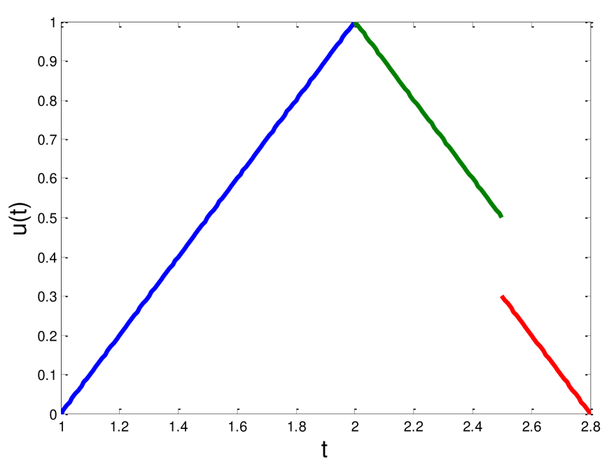
(a) $u$

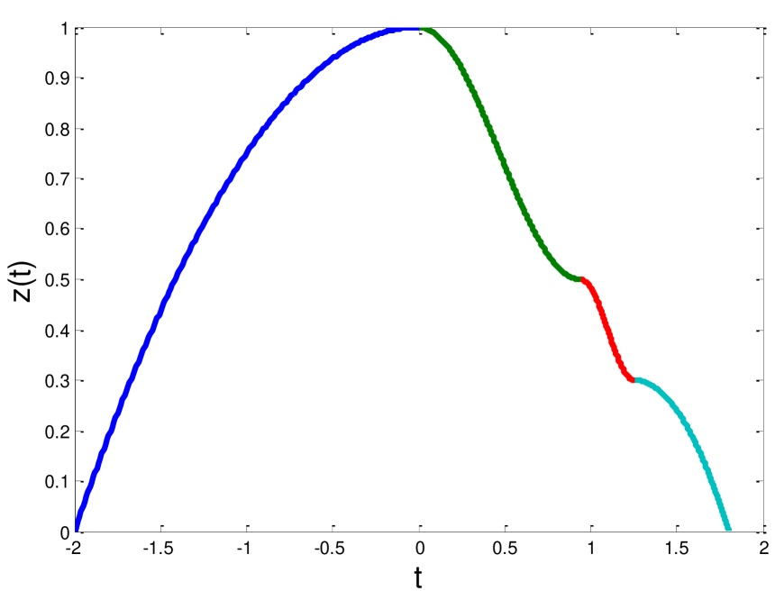
(b) $z$

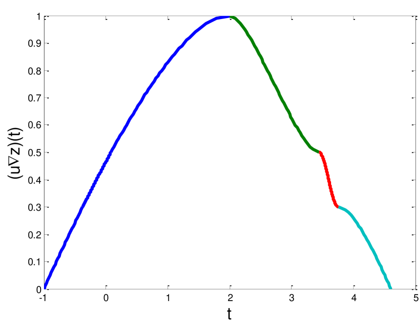
(c) $u\nabla z$

Figure 6: Fuzzy numbers in Example 5.23

Now we use Theorem 5.21 to construct a smoother $z$ for $u$. Observe that the only non-differentiable point of $u$ in $(u^{-}(0),u^{+}(0))$ is $u^{+}(0.5)=2.5$, which is also the only non-continuous point of $u$. Since $u(2.5)=0.5$ and $\lim_{y\to 0.5+}u(y)=0.3$, by conditions (iv-2) and(v-2), it must holds that $z^{\prime}(z^{+}(0.5))=0$ and $z^{\prime}(z^{+}(0.3))=0$. Consider

$$z(t)=\left\{\begin{array}[]{ll}1-t^{2}/4,&\ t\in[-2,0],\\ 0.25\cos(10t/3)+0.75,&\ t\in[0,0.3\pi],\\ 0.4+0.1\cos(10(t-0.3\pi)),&\ t\in[0.3\pi,0.4\pi],\\ 0.3-(t-0.4\pi)^{2},&\ t\in[0.4\pi,0.4\pi+\sqrt{0.3}],\\ 0,&\ t\notin[-2,0.4\pi+\sqrt{0.3}].\end{array}\right.$$

See Fig. 6b for the figure of $z$. It can be checked that $z\in\mathcal{F}_{\mathrm{D}}(\mathbb{R})$ and that

$$z^{\prime}(z^{+}(0.5))=z^{\prime}(0.3\pi)=0,$$

$$z^{\prime}(z^{+}(0.3))=z^{\prime}(0.4\pi)=0.$$

We can see that $u$ and $z$ also satisfy all other conditions in Theorem 5.21. Thus, by Theorem 5.21, $z$ is a smoother of $u$. To validated this assertion, we compute that

$$(u\nabla z)(t)=\left\{\begin{array}[]{ll}t+2(3-t)^{0.5}-3,&\ t\in[-1,2],\\ f(t),&\ t\in[2,0.3\pi+2.5],\\ 2/5-\cos(10t-25)/10,&\ t\in[0.3\pi+2.5,\ 0.4\pi+2.5],\\ 0.4\pi-t+0.5(4t-1.6\pi-9)^{0.5}+2.3,&\ t\in[0.4\pi+2.5,\ 0.4\pi+2.8+0.3^{0.5}],\\ 0,&t\notin[-1,0.4\pi+2.8+0.3^{0.5}]\end{array}\right.$$

where $f$ is the inverse function of $0.3\arccos(4\alpha-3)+3-\alpha$ when $\alpha\in[0.5,1]$. See Fig. 6c for the figure of $u\nabla z$. It can be verified that $u\nabla z\in\mathcal{F}_{\mathrm{D}}(\mathbb{R})$. In fact, it only need to show that $u\nabla z$ is differentiable at points $2$, $0.3\pi+2.5$, and $0.4\pi+2.5$. Use implicit differentiation to take $f^{\prime}$ as follows:

$$f^{\prime}(t)=\left(\frac{-1.2}{\sqrt{1-(4\alpha(t)-3)^{2}}}-1\right)^{-1}.$$

Then $(u\nabla z)_{-}^{\prime}(2)=\frac{d}{dt}(1+0.5(3-t)^{-0.5}\cdot(-1)\cdot 2)|_{t=2}=0$, and $(u\nabla z)_{+}^{\prime}(2)=f^{\prime}(2)=0$. Hence

$$(u\nabla z)^{\prime}(2)=0.$$ (15)

Similarly, it can be computed that

$$(u\nabla z)^{\prime}(0.3\pi+2.5)=0,$$ (16)

$$(u\nabla z)^{\prime}(0.4\pi+2.5)=0.$$ (17)

It now follows from (15), (16), and (17) that $u\nabla z$ is differentiable on $(-1,0.4\pi+2.8+0.3^{0.5})$, i.e, $u\nabla z\in\mathcal{F}_{\mathrm{D}}(\mathbb{R})$. This means that $z$ is a smoother of $u$. From this example we can see how conditions (iv) and (v) take effect.

By using a similar procedure as described in Example 5.23, we can construct a smoother $\zeta$ for $u\in\mathcal{F}(\mathbb{R})$ which has finite number of non-differentiable points. Note that a non-continuous point is also a non-differentiable point, this means that the number of non-continuous points and the number of continuous but non-differentiable points are both finite. First, it picks out all the non-continuous points and continuous but non-differentiable points in $(u^{-}(0),u^{+}(0))$. Based on this, by using conditions (i), (ii), (iv) and (v), we then give some requirements on $\zeta$ which ensure $\zeta$ to be a smoother for $u$. Finally, we use polynomial functions, sine functions and cosine functions to construct a concrete fuzzy number $\zeta\in\mathcal{F}_{\mathrm{D}}(\mathbb{R})$ which meets these requirements. From Theorem 5.21, we know that $\zeta$ is a smoother of $u$. Since the number of non-differentiable points of $u$ is finite, this procedure can be completed in finite steps.

Now we discuss how to construct a smooth fuzzy numbers sequence to approximate a fuzzy number in $\mathcal{F}(\mathbb{R})$. In fact, it can proceed as in the construction of smooth fuzzy numbers sequences for fuzzy numbers in $\mathcal{F}_{\mathrm{C}}(\mathbb{R})$.

Suppose that $u,\zeta\in\mathcal{F}(\mathbb{R})$. From eqs. (10)–(14) and Theorem 5.21, we know that $\zeta$ is a smoother of $u$ is equivalent to $p\cdot\zeta$, $p>0$, are smoothers of $u$. So we have the following statement which shows that, by using the convolution method, it can produce a smooth approximation for an arbitrary fuzzy number with finite non-differentiable points.

Theorem 5.24

Suppose that $u$ is a fuzzy number. If the number of non-differentiable points of $u$ is finite, then there exist smoothers for $u$. Moreover, if $\zeta$ is a smoother of $u$, then $p\cdot\zeta$, $p>0$, are also smoothers of $u$, and

$$d_{\infty}(u,u\nabla(p\cdot\zeta))\leq p\cdot\max\{|\zeta^{+}(0)|,|\zeta^{-}(0)|\}.$$

So $\{u\nabla(p\cdot\zeta)\}$ converges to $u$ according to the supremum metric $d_{\infty}$ as $p\to 0$.

6 Properties of the approximations generated by the convolution method

In this section we discuss the properties of the approximations generated by the convolution method.

We affirm that the convolution method can produce smooth approximations which preserve the core, where an approximation $\{v_{n}\}$ of a fuzzy number $u$ preserves the core means that Core($v_{n}$)=Core($u$) for all $n$. In fact, if a smoother $v$ of $u$ satisfies the condition $[v]_{1}=\{0\}$, then $[p\cdot v]_{1}=\{0\}$, and thus the corresponding approximation $\{u\nabla(\frac{1}{n}\cdot v),n=1,2,\ldots\}$ for the fuzzy number $u$ preserves the core. It is easy to select a smoother $v$ which satisfies the condition $[v]_{1}=\{0\}$. For example, if $w$ is a smoother of a fuzzy number $u$, then we can define $v$ by

$$[v]_{\alpha}=[w^{-}(\alpha)-w^{-}(1),w^{+}(\alpha)-w^{+}(1)]$$

for all $\alpha\in[0,1]$. It can be check that $[v]_{1}=\{0\}$, and that, from Theorems 5.7, 5.15, 5.21, $v$ is also a smoother for $u$.

We also find that the convolution method can generate Lipschitz and smooth approximation, where a Lipschitz approximation is a approximation which is constructed by Lipschitz fuzzy numbers. To show this assertion, we need the following lemma.

Lemma 6.1

Suppose that $u$ is a fuzzy number. Then the following statements are equivalent.
(i)  $u$ is Lipschitz with Lipschitz constant $K$.
(ii)  $|\alpha-\beta|\leq K|u^{-}(\alpha)-u^{-}(\beta)|$ for all $\alpha,\beta\in[u(u^{-}(0)),1]$, and $|\gamma-\delta|\leq K|u^{+}(\gamma)-u^{+}(\delta)|$ for all $\gamma$, $\delta$ in $[u(u^{+}(0)),1]$.
(iii)  $|\alpha-\beta|\leq K|u_{s}^{-}(\alpha)-u^{-}(\beta)|$ for all $\alpha,\beta\in[u(u^{-}(0)),1]$, and $|\gamma-\delta|\leq K|u_{s}^{+}(\gamma)-u^{+}(\delta)|$ for all $\gamma$, $\delta$ in $[u(u^{+}(0)),1]$.

Proof  (i)$\Rightarrow$(ii). If $u$ is Lipschitz with Lipschitz constant $K$, then $u\in\mathcal{F}_{\mathrm{C}}(\mathbb{R})$. Given $\alpha,\beta\in[u(u^{-}(0)),1]$, by Corollary 3.4, $u(u^{-}(\alpha))=\alpha$ and $u(u^{-}(\beta))=\beta$. Thus it follows from $u$ is Lipschitz that

$$|\alpha-\beta|\leq K|u^{-}(\alpha)-u^{-}(\beta)|.$$

Similarly, we can prove that $|\gamma-\delta|\leq K|u^{+}(\gamma)-u^{+}(\delta)|$ for all $\gamma$, $\delta$ in $[u(u^{+}(0)),1]$.

(ii)$\Rightarrow$(iii). Given $\alpha,\beta\in[u(u^{-}(0)),1]$, if $\beta\leq\alpha$, then

$$|\alpha-\beta|\leq K|u^{-}(\alpha)-u^{-}(\beta)|\leq K|u_{s}^{-}(\alpha)-u^{-}(\beta)|.$$

If $\beta>\alpha$, note that $u_{s}^{-}(\alpha)=\lim_{\lambda\to\alpha+}u^{-}(\lambda)$, since

$$|\beta-\lambda|\leq K|u^{-}(\beta)-u^{-}(\lambda)|,$$

let $\lambda\to\alpha+$, then we obtain that

$$|\beta-\alpha|\leq K|u^{-}(\beta)-u_{s}^{-}(\alpha)|.$$

Similarly, we can prove that $|\gamma-\delta|\leq K|u_{s}^{+}(\gamma)-u^{+}(\delta)|$ for all $\gamma$, $\delta$ in $[u(u^{+}(0)),1]$.

(iii)$\Rightarrow$(i). Given $x,y\in[u]_{0}$, put $u(x)=\alpha$ and $u(y)=\beta$. Assume that $\alpha<\beta$ with no loss of generality. Then we have

$$|x-y|\geq\min\{|u_{s}^{-}(\alpha)-u^{-}(\beta)|,\ |u_{s}^{+}(\alpha)-u^{+}(\beta)|\}.$$

From statement (iii),

$$|\alpha-\beta|\leq K|u_{s}^{-}(\alpha)-u^{-}(\beta)|,$$

$$|\alpha-\beta|\leq K|u_{s}^{+}(\alpha)-u^{+}(\beta)|,$$

and thus

$$|u(x)-u(y)|=|\alpha-\beta|\leq K|x-y|.$$

This means that $u$ is Lipschitz with Lipschitz constant $K$. $\quad\Box$

The following theorem shows that the convolution transform can retain the Lipschitz property under an assumption which is general for smoothers.

Theorem 6.2

Suppose that $u$ is a fuzzy number, and that $v$ is a Lipschitz fuzzy number with Lipschitz constant $K$. If $v(v^{-}(0))\leq u(u^{-}(0))$ and $v(v^{+}(0))\leq u(u^{+}(0))$, then $u\nabla v$ is also a Lipschitz fuzzy number.

Proof  Note that, by Lemma 3.11,

$$(u\nabla v)((u\nabla v)^{-}(0))=u(u^{-}(0))\wedge v(v^{-}(0))=v(v^{-}(0)).$$

Given $\alpha$, $\beta$ in $[(u\nabla v)((u\nabla v)^{-}(0)),1]$, then $\alpha$, $\beta$ is also in $[v(v^{-}(0)),1]$. Since $v$ is Lipschitz with Lipschitz constant $K$, it follows from Lemma 6.1 (ii) that

$$|\alpha-\beta|\leq K|v^{-}(\alpha)-v^{-}(\beta)|\leq K|(u\nabla v)^{-}(\alpha)-(u\nabla v)^{-}(\beta)|.$$

Similarly, we can obtain that

$$|\gamma-\delta|\leq K|v^{+}(\gamma)-v^{+}(\delta)|\leq K|(u\nabla v)^{+}(\gamma)-(u\nabla v)^{+}(\delta)|$$

for all $\gamma,\delta\in[(u\nabla v)((u\nabla v)^{+}(0)),1]$. So $u\nabla v$ is also Lipschitz with Lipschitz constant $K$. $\quad\Box$

Since we use polynomial functions, sine functions and cosine functions to construct smoothers, it is easy to make the smoothers to be a Lipschitz fuzzy number. Note that in the construction process of a smoother, it requires that $v(v^{-}(0))=u(u^{-}(0))$ and $v(v^{+}(0))=u(u^{+}(0))$, where $u$ is the original fuzzy number and $v$ is its smoother (see condition (i)). Thus, by Theorems 5.24 and 6.2, we can produce a Lipschitz and smooth approximation for a fuzzy number with finite non-differentiable points. From the above discussions, we can further ensure this Lipschitz and smooth approximation preserves the core at the same time.

Remark 6.3

From Theorems 4.1, 4.2 and 4.3, we know that if $v$ is a smoother for $u\in\mathcal{F}(\mathbb{R})$, then

$$v^{\prime}(v^{-}(\alpha))\geq(u\nabla v)^{\prime}((u\nabla v)^{-}(\alpha)),$$

$$v^{\prime}(v^{+}(\alpha))\geq(u\nabla v)^{\prime}((u\nabla v)^{+}(\alpha)),$$

for all $\alpha\in(0,1]$. It follows immediately that if a smoother $v$ of $u$ is Lipschitz, then $u\nabla v$ is also Lipschitz.

7 Conclusions

This paper discusses how to smooth fuzzy numbers and then construct smooth approximations for fuzzy numbers by using the convolution method. The main contents are illustrated in the following.

1

It shows that how to use the convolution method to produce smooth approximations for fuzzy numbers which have finite non-differentiable points. This type of fuzzy numbers are quite general in real world applications.

2

It further points out that the convolution method can generate smooth and Lipschitz approximations which preserve the core at the same time.

3

The constructing of smoothers is the key step in the construction processes of approximations in the above results. Theorems 5.7, 5.15 and 5.21 provide principles for constructing smoothers, therein conditions are given to ensure that the constructed fuzzy numbers are smoothers for a given type of fuzzy numbers. These conditions are general. In fact, by the conditions in Theorem 5.7, we can judge that the classes of fuzzy numbers $\{w_{p}\}$ and $\{Z_{p}^{f}\}$ introduced in [27, 28] are smoothers for fuzzy numbers in $\mathcal{F}^{0}_{\mathrm{NC}}(\mathbb{R})$. See Remark 5.11 for details.

Appendix A A Proof of Theorem 4.1

We only prove statements (i) and (ii). The remainder statements (iii) -(viii) can be proved in the same way.

Set $v(v^{-}(0))=\alpha_{0}$ and $v(v^{+}(0))=\beta_{0}$, then, by Lemma 3.11,

$$(u\nabla v)((u\nabla v)^{-}(0))\leq\alpha_{0},\ (u\nabla v)((u\nabla v)^{+}(0))\leq\beta_{0},$$

$$(u\nabla v)((u\nabla v)^{-}(\alpha_{0}))=\alpha_{0},\ (u\nabla v)((u\nabla v)^{+}(\beta_{0}))=\beta_{0}.$$

(i)  If $\alpha=\alpha_{0}$, then $v^{-}(\alpha)=v^{-}(\alpha_{0})=v^{-}(0)$. From $v^{\prime}_{-}(v^{-}(0))=0$, we know that $v$ is left-continuous at $v^{-}(0)$. Note that $v(x)=0$ for all $x<v^{-}(0)$, thus $v(v^{-}(0))=0=\alpha_{0}$. Hence $(u\nabla v)((u\nabla v)^{-}(0))=0$, and therefore $(u\nabla v)^{\prime}_{-}((u\nabla v)^{-}(0))=0$.

If $\alpha>\alpha_{0}$, then by $v^{\prime}_{-}(v^{-}(\alpha))=0$, we know that $v$ is left-continuous at $v^{-}(\alpha)$. So, by Proposition 3.1, $v(v^{-}(\alpha))=\alpha$ and hence, by Lemma 3.11, $(u\nabla v)((u\nabla v)^{-}(\alpha))=\alpha$.

Now we prove that $(u\nabla v)^{\prime}_{-}((u\nabla v)^{-}(\alpha))=0$. Note that

$$(u\nabla v)^{\prime}_{-}((u\nabla v)^{-}(\alpha))=\lim_{z\to(u\nabla v)^{-}(\alpha)-}\frac{(u\nabla v)((u\nabla v)^{-}(\alpha))-(u\nabla v)(z)}{(u\nabla v)^{-}(\alpha)-z}.$$

Given $z\in((u\nabla v)^{-}(\alpha_{0}),(u\nabla v)^{-}(\alpha))$, obviously

$$\frac{(u\nabla v)((u\nabla v)^{-}(\alpha))-(u\nabla v)(z)}{(u\nabla v)^{-}(\alpha)-z}\geq 0.$$ (18)

On the other hand, set $(u\nabla v)(z)=\alpha-\delta$, where $\delta>0$, then by Proposition 3.1,

$$z\leq(u\nabla v)_{s}^{-}(\alpha-\delta),$$

and thus

$$\frac{(u\nabla v)((u\nabla v)^{-}(\alpha))-(u\nabla v)(z)}{(u\nabla v)^{-}(\alpha)-z}$$

$$\leq\frac{\alpha-(\alpha-\delta)}{(u\nabla v)^{-}(\alpha)-(u\nabla v)_{s}^{-}(\alpha-\delta)}$$

$$=\frac{\delta}{u^{-}(\alpha)-u_{s}^{-}(\alpha-\delta)+v^{-}(\alpha)-v_{s}^{-}(\alpha-\delta)}$$

$$\leq\frac{\delta}{v^{-}(\alpha)-v_{s}^{-}(\alpha-\delta)}.$$ (19)

By Proposition 3.1, it holds that

$$\lim_{x\to v_{s}^{-}(\alpha-\delta)-}v(x)\leq\alpha-\delta,$$

and therefore

$$\lim_{x\to v_{s}^{-}(\alpha-\delta)-}\frac{v(v^{-}(\alpha))-v(x)}{v^{-}(\alpha)-x}\geq\frac{\alpha-(\alpha-\delta)}{v^{-}(\alpha)-v_{s}^{-}(\alpha-\delta)}=\frac{\delta}{v^{-}(\alpha)-v_{s}^{-}(\alpha-\delta)}.$$ (20)

Given $\varepsilon>0$, since $v^{\prime}_{-}(v^{-}(\alpha))=0$, there is a $\xi(\varepsilon)>0$ such that for all $y\in(v^{-}(\alpha)-\xi,v^{-}(\alpha))$, it holds that

$$\frac{v(v^{-}(\alpha))-v(y)}{v^{-}(\alpha)-y}=\frac{\alpha-v(y)}{v^{-}(\alpha)-y}\leq\varepsilon.$$ (21)

Hence, by (21), if $v^{-}(\alpha)-v_{s}^{-}(\alpha-\delta)<\xi$, then

$$\lim_{x\to v_{s}^{-}(\alpha-\delta)-}\frac{v(v^{-}(\alpha))-v(x)}{v^{-}(\alpha)-x}\leq\varepsilon,$$ (22)

and thus, combined with (20) and (22), we have

$$\frac{\delta}{v^{-}(\alpha)-v_{s}^{-}(\alpha-\delta)}\leq\varepsilon.$$ (23)

So if $(u\nabla v)^{-}(\alpha)-z<\xi$, then $v^{-}(\alpha)-v_{s}^{-}(\alpha-\delta)<(u\nabla v)^{-}(\alpha)-(u\nabla v)_{s}^{-}(\alpha-\delta)<(u\nabla v)^{-}(\alpha)-z<\xi$, hence, by (19) and (23), we get that

$$\frac{(u\nabla v)((u\nabla v)^{-}(\alpha))-(u\nabla v)(z)}{(u\nabla v)^{-}(\alpha)-z}<\varepsilon,$$

from the arbitrariness of $\varepsilon>0$ and (18), we have

$$(u\nabla v)_{-}^{\prime}((u\nabla v)^{-}(\alpha))=0.$$

So statement (i) holds.

(ii)  Since $v(v^{-}(\alpha))=\beta$, we have $\beta\geq\alpha$, and $v^{-}(\alpha)=v^{-}(\beta)$. This implies that $(u\nabla v)((u\nabla v)^{-}(\beta))=\beta$.

Now we show that $(u\nabla v)_{+}^{\prime}((u\nabla v)^{-}(\beta))=0$ when $v^{\prime}_{+}(v^{-}(\alpha))=0$. If $(u\nabla v)^{-}(\beta)<(u\nabla v)_{s}^{-}(\beta)$, then it follows immediately that $(u\nabla v)_{+}^{\prime}((u\nabla v)^{-}(\beta))=0$.

In the following, we suppose that $(u\nabla v)^{-}(\beta)=(u\nabla v)_{s}^{-}(\beta)$, then $u^{-}(\beta)=u_{s}^{-}(\beta)$ and $v^{-}(\beta)=v_{s}^{-}(\beta)$. Note that

$$(u\nabla v)^{\prime}_{+}((u\nabla v)^{-}(\beta))=\lim_{z\to(u\nabla v)^{-}(\beta)+}\frac{(u\nabla v)(z)-(u\nabla v)((u\nabla v)^{-}(\beta))}{z-(u\nabla v)^{-}(\beta)}.$$

The proof is divided into two cases.

Case (A)  $\beta<1$.

In this case, obviously,

$$\liminf_{z\to(u\nabla v)^{-}(\beta)+}\frac{(u\nabla v)(z)-(u\nabla v)((u\nabla v)^{-}(\beta))}{z-(u\nabla v)^{-}(\beta)}\geq 0.$$ (24)

Given $z\in((u\nabla v)^{-}(\beta),(u\nabla v)^{-}(1))$, set $(u\nabla v)(z)=\beta+\delta$, where $\delta>0$, then by Proposition 3.1,

$$z\geq(u\nabla v)^{-}(\beta+\delta),$$

and thus

$$\frac{(u\nabla v)(z)-(u\nabla v)((u\nabla v)^{-}(\beta))}{z-(u\nabla v)^{-}(\beta)}$$

$$\leq \frac{(u\nabla v)(z)-\beta}{(u\nabla v)^{-}(\beta+\delta)-(u\nabla v)^{-}(\beta)}$$

$$= \frac{\delta}{u^{-}(\beta+\delta)-u^{-}(\beta)+v^{-}(\beta+\delta)-v^{-}(\beta)}$$

$$\leq \frac{\delta}{v^{-}(\beta+\delta)-v^{-}(\beta)}$$

$$\leq \frac{v(v^{-}(\beta+\delta))-v(v^{-}(\beta))}{v^{-}(\beta+\delta)-v^{-}(\beta)}.$$ (25)

Let $z\to(u\nabla v)^{-}(\beta)+$, then $\delta\to 0+$. It thus follows from (25) that

$$\limsup_{z\to(u\nabla v)^{-}(\beta)+}\frac{(u\nabla v)(z)-(u\nabla v)((u\nabla v)^{-}(\beta))}{z-(u\nabla v)^{-}(\beta)}$$

$$\leq\lim_{\delta\to 0+}\frac{v(v^{-}(\beta+\delta))-v(v^{-}(\beta))}{v^{-}(\beta+\delta)-v^{-}(\beta)}$$

$$=v^{\prime}_{+}(v^{-}(\beta))=0,$$

and then, combined with (24), we know

$$(u\nabla v)^{\prime}_{+}((u\nabla v)^{-}(\beta))=0.$$

Case (B)  $\beta=1$.

In this case, if $(u\nabla v)^{-}(1)<(u\nabla v)^{+}(1)$, then $(u\nabla v)^{\prime}_{+}((u\nabla v)^{-}(1))=0$. If $(u\nabla v)^{-}(1)=(u\nabla v)^{+}(1)$, then $u^{-}(1)=u^{+}(1)$ and $v^{-}(1)=v^{+}(1)$. So,

$$(u\nabla v)^{\prime}_{+}((u\nabla v)^{-}(1))=(u\nabla v)^{\prime}_{+}((u\nabla v)^{+}(1))=\lim_{z\to(u\nabla v)^{+}(1)+}\frac{(u\nabla v)((u\nabla v)^{+}(1))-(u\nabla v)(z)}{(u\nabla v)^{+}(1)-z}.$$

It is easy to see that

$$\limsup_{z\to(u\nabla v)^{+}(1)+}\frac{(u\nabla v)((u\nabla v)^{+}(1))-(u\nabla v)(z)}{(u\nabla v)^{+}(1)-z}=\limsup_{z\to(u\nabla v)^{+}(1)+}\frac{1-(u\nabla v)(z)}{(u\nabla v)^{+}(1)-z}\leq 0.$$ (26)

On the other hand, given $\varepsilon>0$, note that $v^{\prime}_{+}(v^{+}(1))=v^{\prime}_{+}(v^{-}(1))=0$, so there is a $\xi>0$ such that for each $y\in(v^{+}(1),v^{+}(1)+\xi)$,

$$\frac{1-v(y)}{v^{+}(1)-y}\geq-\varepsilon,$$

proceed as in statement (i), we can get that if $z-(u\nabla v)^{+}(1)<\xi$, then

$$\frac{1-(u\nabla v)(z)}{(u\nabla v)^{+}(1)-z}\geq-\varepsilon,$$

and hence from the arbitrariness of $\varepsilon$, we know

$$\liminf_{z\to(u\nabla v)^{+}(1)+}\frac{(u\nabla v)((u\nabla v)^{+}(1))-(u\nabla v)(z)}{(u\nabla v)^{+}(1)-z}=\liminf_{z\to(u\nabla v)^{+}(1)+}\frac{1-(u\nabla v)(z)}{(u\nabla v)^{+}(1)-z}\geq 0.$$ (27)

Combined with (26) and (27), we obtain that

$$(u\nabla v)^{\prime}_{+}((u\nabla v)^{+}(1))=0.$$

So statement (ii) holds. $\quad\Box$

Appendix B B Proof of Theorem 4.2

To prove Theorem 4.2, we need following lemmas and corollary. Therein, it shows that the derivatives of a fuzzy number can be computed by calculations which are determined by its values at the endpoints of $\alpha$-cuts and strong-$\alpha$-cuts.

Lemma B.1

Let $u\in\mathcal{F}(\mathbb{R})$. Set $u(u^{-}(0))=\alpha_{0}$ and $u(u^{+}(0))=\beta_{0}$. Then the following statements hold.
(i)  Given $\alpha\in(\alpha_{0},1]$, then $u^{\prime}_{-}(u^{-}(\alpha))=\varphi$ if and only if

$$\lim_{\gamma\to\alpha-}\frac{u(u^{-}(\alpha))-\gamma}{u^{-}(\alpha)-u^{-}(\gamma)}=\lim_{\gamma\to\alpha-}\frac{u(u^{-}(\alpha))-\gamma}{u^{-}(\alpha)-u_{s}^{-}(\gamma)}=\varphi.$$

(ii)  Given $\beta\in(\beta_{0},1]$, then $u^{\prime}_{+}(u^{+}(\beta))=\psi$ if and only if

$$\lim_{\lambda\to\beta-}\frac{u(u^{+}(\beta))-\lambda}{u^{+}(\beta)-u^{+}(\lambda)}=\lim_{\lambda\to\beta-}\frac{u(u^{+}(\beta))-\lambda}{u^{+}(\beta)-u_{s}^{+}(\lambda)}=\psi.$$

Proof  (i)  Sufficiency.  Suppose that

$$\lim_{\gamma\to\alpha-}\frac{u(u^{-}(\alpha))-\gamma}{u^{-}(\alpha)-u^{-}(\gamma)}=\lim_{\gamma\to\alpha-}\frac{u(u^{-}(\alpha))-\gamma}{u^{-}(\alpha)-u_{s}^{-}(\gamma)}=\varphi,$$

we show that

$$u^{\prime}_{-}(u^{-}(\alpha))=\lim_{z\to u^{-}(\alpha)-}\frac{u(u^{-}(\alpha))-u(z)}{u^{-}(\alpha)-z}=\varphi.$$

In fact, given $z\in(u^{-}(0),u^{-}(\alpha))$, suppose that $u(z)=\gamma$, then $\gamma<\alpha$, and, by Proposition 3.1,

$$u^{-}(\gamma)\leq z\leq u_{s}^{-}(\gamma),$$

hence

$$\frac{u(u^{-}(\alpha))-\gamma}{u^{-}(\alpha)-u^{-}(\gamma)}\leq\frac{u(u^{-}(\alpha))-u(z)}{u^{-}(\alpha)-z}\leq\frac{u(u^{-}(\alpha))-\gamma}{u^{-}(\alpha)-u_{s}^{-}(\gamma)},$$

note that if $\gamma\to\alpha-$, then $z\to u^{-}(\alpha)-$, and thus

$$\lim_{\gamma\to\alpha-}\frac{u(u^{-}(\alpha))-\gamma}{u^{-}(\alpha)-u^{-}(\gamma)}=\lim_{z\to u^{-}(\alpha)-}\frac{u(u^{-}(\alpha))-u(z)}{u^{-}(\alpha)-z}=\lim_{\gamma\to\alpha-}\frac{u(u^{-}(\alpha))-\gamma}{u^{-}(\alpha)-u_{s}^{-}(\gamma)}=\varphi,$$

i.e.

$$u^{\prime}_{-}(u^{-}(\alpha))=\varphi.$$

Necessity.   Suppose that $u^{\prime}_{-}(u^{-}(\alpha))=\varphi$, we prove that

$$\lim_{\gamma\to\alpha-}\frac{u(u^{-}(\alpha))-\gamma}{u^{-}(\alpha)-u^{-}(\gamma)}=\lim_{\gamma\to\alpha-}\frac{u(u^{-}(\alpha))-\gamma}{u^{-}(\alpha)-u_{s}^{-}(\gamma)}=\varphi.$$

Now we use a trick which also is used in the proof of Lemma 4.1. Given $\varepsilon>0$, since $u^{\prime}_{-}(u^{-}(\alpha))=\varphi$, there is a $\xi>0$, such that for all $y\in(u^{-}(\alpha)-\xi,u^{-}(\alpha))$,

$$\varphi-\varepsilon\leq\frac{u(u^{-}(\alpha))-u(y)}{u^{-}(\alpha)-y}\leq\varphi+\varepsilon,$$

notice that, for each $\beta$,

$$\lim_{x\to u^{-}(\beta)-}u(x)\leq\beta\leq u(u^{-}(\beta)),$$

and hence if $0<u^{-}(\alpha)-u^{-}(\gamma)<\xi$, then

$$\varphi+\varepsilon\geq\lim_{x\to u^{-}(\gamma)-}\frac{u(u^{-}(\alpha))-u(x)}{u^{-}(\alpha)-x}\geq\frac{u(u^{-}(\alpha))-\gamma}{u^{-}(\alpha)-u^{-}(\gamma)}\geq\frac{u(u^{-}(\alpha))-u(u^{-}(\gamma))}{u^{-}(\alpha)-u^{-}(\gamma)}\geq\varphi-\varepsilon,$$

now let $\gamma\to\alpha-$, we obtain that

$$\lim_{\gamma\to\alpha-}\frac{u(u^{-}(\alpha))-\gamma}{u^{-}(\alpha)-u^{-}(\gamma)}=\varphi=u^{\prime}_{-}(u^{-}(\alpha)).$$

Similarly, we can prove that

$$\lim_{\gamma\to\alpha-}\frac{u(u^{-}(\alpha))-\gamma}{u^{-}(\alpha)-u_{s}^{-}(\gamma)}=\varphi=u^{\prime}_{-}(u^{-}(\alpha)).$$

(ii)  Since $u^{\prime}_{+}(u^{+}(\beta))=\psi$, we know that if $\lambda\to\beta-$, then $u^{+}(\lambda)\to u^{+}(\beta)+$. The remainder proof is similarly to the proof of statement (i) $\quad\Box$

Corollary B.2

Let $u\in\mathcal{F}(\mathbb{R})$. Set $u(u^{-}(0))=\alpha_{0}$ and $u(u^{+}(0))=\beta_{0}$. Then the following statements hold.
(i)  Given $\alpha\in(\alpha_{0},1]$, then $u^{\prime}_{-}(u^{-}(\alpha))=\varphi$ if and only if $u(u^{-}(\alpha))=\alpha$, and

$$\lim_{\gamma\to\alpha-}\frac{\alpha-\gamma}{u^{-}(\alpha)-u^{-}(\gamma)}=\lim_{\gamma\to\alpha-}\frac{\alpha-\gamma}{u^{-}(\alpha)-u_{s}^{-}(\gamma)}=\varphi.$$

(ii)  Given $\beta\in(\beta_{0},1]$, then $u^{\prime}_{+}(u^{+}(\beta))=\psi$ if and only if $u(u^{+}(\beta))=\beta$, and

$$\lim_{\lambda\to\beta-}\frac{\beta-\lambda}{u^{+}(\beta)-u^{+}(\lambda)}=\lim_{\lambda\to\beta-}\frac{\beta-\lambda}{u^{+}(\beta)-u_{s}^{+}(\lambda)}=\psi.$$

Proof  Note that if $u^{\prime}_{-}(u^{-}(\alpha))=\varphi$, then $u$ is left-continuous at $u^{-}(\alpha)$, and then

$$\lim_{x\to u^{-}(\alpha)-}u(x)=u(u^{-}(\alpha))=\alpha.$$

Similarly, if $u^{\prime}_{+}(u^{+}(\beta))=\psi$, then

$$\lim_{x\to u^{+}(\beta)+}u(x)=u(u^{+}(\beta))=\beta.$$

So the desired results follow immediately from Lemma B.1. $\quad\Box$

Lemma B.3

Let $u\in\mathcal{F}(\mathbb{R})$. Then the following statements hold.
(i)  Given $u^{-}(\alpha)\in[u^{-}(0),u^{-}(1))$, set $u(u^{-}(\alpha))=\rho$, then $u^{\prime}_{+}(u^{-}(\alpha))=\phi$ is equivalent to

$$\lim_{\gamma\to\rho+}\frac{\rho-\gamma}{u^{-}(\alpha)-u^{-}(\gamma)}=\lim_{\gamma\to\rho+}\frac{\rho-\gamma}{u^{-}(\alpha)-u_{s}^{-}(\gamma)}=\phi.$$

(ii)  Given $u^{+}(\beta)\in(u^{+}(1),u^{+}(0)]$, set $u(u^{+}(\beta))=\sigma$, then $u^{\prime}_{-}(u^{+}(\beta))=\omega$ is equivalent to

$$\lim_{\gamma\to\sigma+}\frac{\sigma-\gamma}{u^{+}(\beta)-u^{+}(\gamma)}=\lim_{\gamma\to\sigma+}\frac{\sigma-\gamma}{u^{+}\beta)-u_{s}^{+}(\gamma)}=\omega.$$

Proof  (i)  Since $u(u^{-}(\alpha))=\rho$, we know that $u^{-}(\alpha)=u^{-}(\rho)$ and $\rho<1$. The proof is divided into two cases.

Case (A)   $u^{-}(\alpha)<u_{s}^{-}(\alpha)$.

In this case, $u^{\prime}_{+}(u^{-}(\alpha))=0$, and

$$\lim_{\gamma\to\rho+}\frac{\rho-\gamma}{u^{-}(\alpha)-u^{-}(\gamma)}=\lim_{\gamma\to\rho+}\frac{\rho-\gamma}{u^{-}(\alpha)-u_{s}^{-}(\gamma)}=\frac{0}{u^{-}(\alpha)-u_{s}^{-}(\alpha)}=0,$$

so the statement holds.

Case (B)  $u^{-}(\alpha)=u_{s}^{-}(\alpha)$.

In this cases, $u^{-}(\gamma)\to u^{-}(\alpha)+$ as $\gamma\to\rho+$. The rest of the proof is similar to the proof of statement (i) in Lemma B.1.

(ii)  The proof is similar to statement (i). $\quad\Box$

Proof of Theorem 4.2. (i)  Set $\alpha_{0}=u(u^{-}(0))$ and $\alpha_{1}=v(v^{-}(0))$. Since $u_{-}^{\prime}(u^{-}(\alpha))=\varphi>0$ and $v_{-}^{\prime}(v^{-}(\alpha))=\psi>0$, we know that $\alpha>\max\{\alpha_{0},\alpha_{1}\}$, and

$$\lim_{x\to u^{-}(\alpha)-}u(x)=u(u^{-}(\alpha))=\alpha,$$

$$\lim_{y\to v^{-}(\alpha)-}v(y)=v(v^{-}(\alpha))=\alpha,$$

$$(u\nabla v)((u\nabla v)^{-}(\alpha))=\alpha,$$ (28)

thus $\alpha>(u\nabla v)((u\nabla v)^{-}(0))=\min\{\alpha_{0},\alpha_{1}\}$. To prove $(u\nabla v)_{-}^{\prime}((u\nabla v)^{-}(\alpha))=(\varphi^{-1}+\psi^{-1})^{-1}$, by Corollary B.2 and (28), we only need to show that

$$\lim_{\gamma\to\alpha-}\frac{\alpha-\gamma}{(u\nabla v)^{-}(\alpha)-(u\nabla v)^{-}(\gamma)}=\lim_{\gamma\to\alpha-}\frac{\alpha-\gamma}{(u\nabla v)^{-}(\alpha)-(u\nabla v)_{s}^{-}(\gamma)}=(\varphi^{-1}+\psi^{-1})^{-1}.$$

In fact,

$$\lim_{\gamma\to\alpha-}\frac{\alpha-\gamma}{(u\nabla v)^{-}(\alpha)-(u\nabla v)^{-}(\gamma)}$$

$$=\lim_{\gamma\to\alpha-}\frac{\alpha-\gamma}{u^{-}(\alpha)+v^{-}(\alpha)-(u^{-}(\gamma)+v^{-}(\gamma))}$$

$$=\lim_{\gamma\to\alpha-}\frac{1}{\frac{u^{-}(\alpha)-u^{-}(\gamma)}{\alpha-\gamma}+\frac{v^{-}(\alpha)-v^{-}(\gamma)}{\alpha-\gamma}}.$$ (29)

Since $u_{-}^{\prime}(u^{-}(\alpha))=\varphi>0$ and $v_{-}^{\prime}(v^{-}(\alpha))=\psi>0$, by Corollary B.2, we have

$$\lim_{\gamma\to\alpha-}\frac{u^{-}(\alpha)-u^{-}(\gamma)}{\alpha-\gamma}=\varphi^{-1},$$

$$\lim_{\gamma\to\alpha-}\frac{v^{-}(\alpha)-v^{-}(\gamma)}{\alpha-\gamma}=\psi^{-1},$$

and thus, combined with (29), we get

$$\lim_{\gamma\to\alpha-}\frac{\alpha-\gamma}{(u\nabla v)^{-}(\alpha)-(u\nabla v)^{-}(\gamma)}=(\varphi^{-1}+\psi^{-1})^{-1}.$$

Similarly, we can obtain

$$\lim_{\gamma\to\alpha-}\frac{\alpha-\gamma}{(u\nabla v)^{-}(\alpha)-(u\nabla v)_{s}^{-}(\gamma)}=(\varphi^{-1}+\psi^{-1})^{-1}.$$

So statement (i) is proved.

(ii)  Since $u(u^{-}(\alpha))=v(v^{-}(\alpha))=\beta$, we know that $u^{-}(\alpha)=u^{-}(\beta)$, $v^{-}(\alpha)=v^{-}(\beta),$ and then

$$(u\nabla v)((u\nabla v)^{-}(\beta))=\beta.$$

Note that $u_{+}^{\prime}(u^{-}(\alpha))=\varphi>0$ and $v_{+}^{\prime}(v^{-}(\alpha))=\psi>0$, so $u^{-}(\alpha)<u^{-}(1)$ and $v^{-}(\alpha)<v^{-}(1)$ , and thus

$$\alpha\leq\beta<1.$$

To prove that

$$(u\nabla v)_{+}^{\prime}((u\nabla v)^{-}(\beta))=(\varphi^{-1}+\psi^{-1})^{-1},$$

by Lemma B.3, we only need to show that

$$\lim_{\gamma\to\beta+}\frac{\beta-\gamma}{(u\nabla v)^{-}(\beta)-(u\nabla v)^{-}(\gamma)}=\lim_{\gamma\to\beta+}\frac{\beta-\gamma}{(u\nabla v)^{-}(\beta)-(u\nabla v)_{s}^{-}(\gamma)}=(\varphi^{-1}+\psi^{-1})^{-1}.$$

In fact, reasoning as in the proof of statement (i), we obtain

$$\lim_{\gamma\to\beta+}\frac{\beta-\gamma}{(u\nabla v)^{-}(\beta)-(u\nabla v)^{-}(\gamma)}$$

$$=\lim_{\gamma\to\beta+}\frac{\beta-\gamma}{u^{-}(\beta)+v^{-}(\beta)-(u^{-}(\gamma)+v^{-}(\gamma))}$$

$$=\lim_{\gamma\to\beta+}\frac{1}{\frac{u^{-}(\beta)-u^{-}(\gamma)}{\beta-\gamma}+\frac{v^{-}(\beta)-v^{-}(\gamma)}{\beta-\gamma}}$$

$$=(\varphi^{-1}+\psi^{-1})^{-1}.$$

Similarly, we can get

$$\lim_{\gamma\to\beta+}\frac{\beta-\gamma}{(u\nabla v)^{-}(\beta)-(u\nabla v)_{s}^{-}(\gamma)}=(\varphi^{-1}+\psi^{-1})^{-1}.$$

So statement (ii) is proved.

(iii)  Since $u(u^{-}(\alpha))=\beta$, and $v(v^{-}(\alpha))=\gamma>\beta$, we know that $\alpha\leq\beta<\gamma$, and

$$u^{-}(\alpha)=u^{-}(\beta)<u^{-}(1),$$

$$v^{-}(\alpha)=v^{-}(\gamma),$$

$$(u\nabla v)((u\nabla v)^{-}(\beta))=\beta<1.$$

Note that $v^{-}(\lambda)=v^{-}(\alpha)$ for all $\lambda\in[\alpha,\gamma]$, hence

$$(u\nabla v)^{-}(\rho)=u^{-}(\rho)+v^{-}(\rho)=u^{-}(\rho)+v^{-}(\beta)$$

for each $\rho\in[\beta,\gamma]$, and thus

$$\lim_{\theta\to\beta+}\frac{\beta-\theta}{(u\nabla v)^{-}(\beta)-(u\nabla v)^{-}(\theta)}$$

$$=\lim_{\theta\to\beta+}\frac{\beta-\theta}{u^{-}(\beta)+v^{-}(\beta)-(u^{-}(\theta)+v^{-}(\beta))}$$

$$=\lim_{\theta\to\beta+}\frac{\beta-\theta}{u^{-}(\beta)-u^{-}(\theta)}$$

$$=u^{\prime}_{+}(u^{-}(\beta))=\varphi.$$ (30)

Similarly, from $v_{s}^{-}(\lambda)=v^{-}(\alpha)$ for all $\lambda\in[\alpha,\gamma)$, we get

$$(u\nabla v)_{s}^{-}(\rho)=u_{s}^{-}(\rho)+v_{s}^{-}(\rho)=u_{s}^{-}(\rho)+v^{-}(\beta)$$

for each $\rho\in[\beta,\gamma)$, and thus

$$\lim_{\theta\to\beta+}\frac{\beta-\theta}{(u\nabla v)^{-}(\beta)-(u\nabla v)_{s}^{-}(\theta)}$$

$$=\lim_{\theta\to\beta+}\frac{\beta-\theta}{u^{-}(\beta)+v^{-}(\beta)-(u_{s}^{-}(\theta)+v^{-}(\beta))}$$

$$=\lim_{\theta\to\beta+}\frac{\beta-\theta}{u^{-}(\beta)-u_{s}^{-}(\theta)}$$

$$=u^{\prime}_{+}(u^{-}(\beta))=\varphi.$$ (31)

Now it follows from Lemma B.3, (30) and (31) that $(u\nabla v)_{+}^{\prime}((u\nabla v)^{-}(\beta))=\varphi$.

(iv)  We assert that $u^{-}(\alpha)>u^{-}(0)$. On the contrary, if $u^{-}(\alpha)=u^{-}(0)$, then from $u_{-}^{\prime}(u^{-}(\alpha))=\varphi$, we know $u(u^{-}(\alpha))=\alpha=u(u^{-}(0))=0$. Note that $\lim_{y\to v^{-}(\alpha)-}v(y)=\lambda<\alpha$, this yields that $\lambda<0$, which is a contradiction.

Set $u(u^{-}(0))=\alpha_{0}$, then $u^{-}(\alpha_{0})=u^{-}(0)$, and hence $u^{-}(\alpha)>u^{-}(\alpha_{0})$. This implies that $\alpha>\alpha_{0}$. Since $u_{-}^{\prime}(u^{-}(\alpha))=\varphi$, we know that $u(u^{-}(\alpha))=\alpha$, and thus

$$(u\nabla w)((u\nabla w)^{-}(\alpha))=\alpha.$$

By $\lim_{y\to v^{-}(\alpha)-}v(y)=\lambda<\alpha$, we get that

$$v^{-}(\rho)=v^{-}(\alpha)$$

for all $\rho\in(\lambda,\alpha]$, and hence

$$(u\nabla v)^{-}(\rho)=u^{-}(\rho)+v^{-}(\rho)=u^{-}(\rho)+v^{-}(\alpha)$$

for each $\rho\in(\lambda,\alpha]$. Thus

$$\lim_{\rho\to\alpha-}\frac{\alpha-\rho}{(u\nabla v)^{-}(\alpha)-(u\nabla v)^{-}(\rho)}$$

$$=\lim_{\rho\to\alpha-}\frac{\alpha-\rho}{u^{-}(\alpha)+v^{-}(\alpha)-(u^{-}(\rho)+v^{-}(\alpha))}$$

$$=\lim_{\rho\to\alpha-}\frac{\alpha-\rho}{u^{-}(\alpha)-u^{-}(\rho)}$$

$$=u^{\prime}_{-}(u^{-}(\alpha))=\varphi.$$ (32)

Similarly, note that $v_{s}^{-}(\rho)=v^{-}(\alpha)$ for all $\rho\in[\lambda,\alpha)$, we get

$$(u\nabla v)_{s}^{-}(\rho)=u_{s}^{-}(\rho)+v_{s}^{-}(\rho)=u_{s}^{-}(\rho)+v^{-}(\alpha)$$

for each $\rho\in[\lambda,\alpha)$, and thus

$$\lim_{\rho\to\alpha-} \frac{\alpha-\rho}{(u\nabla v)^{-}(\alpha)-(u\nabla v)_{s}^{-}(\rho)}$$

$$= \lim_{\rho\to\alpha-}\frac{\alpha-\rho}{u^{-}(\alpha)+v^{-}(\alpha)-(u_{s}^{-}(\rho)+v^{-}(\alpha))}$$

$$= \lim_{\rho\to\alpha-}\frac{\alpha-\rho}{u^{-}(\alpha)-u_{s}^{-}(\rho)}$$

$$= u^{\prime}_{-}(u^{-}(\alpha))=\varphi.$$ (33)

Now it follows from Corollary B.2, (32) and (33) that $(u\nabla v)_{-}^{\prime}((u\nabla v)^{-}(\alpha))=\varphi$. $\quad\Box$

References

[1] S. Abbasbandy, B. Asady,
The nearest trapezoidal fuzzy number
to a fuzzy quantity,
Appl. Math. Comput. 156 (2004) 381-386.
[2]
A. Ban,
On the nearest parametric approximation of a fuzzy
number-revisited,
Fuzzy Sets Syst. 160 (2009) 3027-3047.
[3]
A. Ban,
Triangular and parametric approximations of fuzzy numbers-inadvertences and corrections,
Fuzzy Sets Syst. 160 (2009) 3048-3058.
[4] A.I. Ban, L. Coroianu,
Metric properties of the nearest extended parametric fuzzy number and applications,
Int. J. Approx. Reason. 52 (2011) 488-500.
[5] S. Chanas, On the interval approximation of a fuzzy number, Fuzzy Sets Syst. 122 (2001) 353-356.
[6] G. Castellano, A.M. Fanelli, C. Mencar,
An empirical risk functional
to improve learning in a fuzzy-neuro classifier,
IEEE Trans. Systems Man Cybernet. 34 (2004) 725-731.
[7] I.L. Colling, P.E. Kloeden,
Continuous approximation of fuzzy sets,
J. Fuzzy Math. 3(2) (1995) 449-453.
[8]
L. Coroianu, L. Stefanini,
General approximation of fuzzy numbers by F-transform,
Fuzzy Sets Syst. (2015)
http://dx.doi.org/10.1016/j.fss.2015.03.015.
[9] L. Coroianu, S.G. Gal, B. Bede,