The potential impact of turbulent velocity fluctuations on drizzle formation in Cumulus clouds in an idealized 2D setup

Abstract

This article discusses a potential impact of turbulent velocity fluctuations of the air on a drizzle formation in Cumulus clouds. Two different representations of turbulent velocity fluctuations for a microphysics formulated in a Lagrangian framework are discussed - random walk model and the interpolation, and its effect on microphysical properties of the cloud investigated.

Turbulent velocity fluctuations significantly enhances velocity differences between colliding droplets, especially those having small sizes. As a result drizzle forms faster in simulations including a representation of turbulence. Both representations of turbulent velocity fluctuations, random walk and interpolation, have similar effect on droplet spectrum evolution, but interpolation of the velocity does account for a possible anisotropy in the air velocity.

All discussed simulations show relatively large standard deviation ($\sim$1${\mu}m$) of the cloud droplet distribution from the onset of cloud formation is observed. Because coalesence processes aerosol inside cloud droplets, detail information about aerosol is available. Results from numerical simulations show that changes in aerosol spectrum due to aerosol processing during droplet coalescence are relatively small during $\sim$20 min. of the cloud evolution simulated with numerical model.

Drizzle forms initially near the cloud edge, either near the cloud top, where the mass of water is the largest, or near the entrainment eddies.

1 Introduction

One of the unresolved problems in cloud physics is drizzle formation in a warm (ice free) clouds. Early modelling studies using Lagrangian parcel models Warner (1969b), Bartlett and Jonas (1972) demonstrated that condensational growth leads to a very narrow droplet spectrum, contrary to the observations, where the droplet spectrum inside the cloud was relatively broad e.g. Warner (1969a). A narrow droplet spectrum makes collision between droplets inefficient and as a result it takes a long time to switch from a condensational to a coagulational droplet growths. Observations show, that development of precipitation in the clouds may be rapid e.g. Goke et al. (2007) which couldn’t be explained by the modelling results. Several mechanisms to explain this discrepancy between numerical model and observations were proposed and were reviewed by Beard and Ochs (1993).

Undoubtedly representation of the cloud formation process by a parcel model is an approximation. Nevertheless attempts were made over the time to explain the width of the cloud droplet spectrum in clouds using this approach. Yum and Hudson (2005) showed that a much broader droplet spectrum can be obtained when instead of one vertical velocity, a velocity distribution is used. Another approach was utilized by Bewley and Lasher-Trapp (2005) and Lasher-Trapp et al. (2005), who used a velocity field from a bulk model to derive trajectories for the parcel models. For both these approaches droplet spectra broader than predicted by a single parcel were reported, however, in these approaches the microphysics is separated from dynamics and thermodynamics of the Eulerian model.

The use of the bin models Grabowski (1989), Kogan (1991), Feingold et al. (1994), Ackerman et al. (1995), Khain et al. (2004), Leroy et al. (2009), Ovchinnikov and Easter (2010), Blyth et al. (2013), Wyszogrodzki et al. (2013), where droplet spectrum is represented as a continuous function, made the problem of the transition from condensational to coagulational disappear. Even very high resolution (in bin sizes) parcel models with bin microphysics are capable of producing precipitation Cooper et al. (1997), Pinsky and Khain (2002) independent of whether turbulent enhancement is or is not taken into account. It’s not clear, however, whether the rain forms in these models due to physical processes or numerical errors associated with the numerical solution of the condensational growth and collision or the physics itself, since detailed comparisons between Eulerian (bin) and Lagrangian models were never to our knowledge reported.

In the recent years a new approach to microphysics formulated in Lagrangian framework was proposed for both warm rain Andrejczuk et al. (2008, 2010), Shima et al. (2009), Riechelmann et al. (2012) and ice clouds Solch and Karcher (2010) . In this approach dynamics and thermodynamics are represented in the traditional Eulerian framework, whilst microphysics is represented in a Lagrangian framework with two way interactions between Eulerian and Lagrangian parts. Lagrangian microphysics tracks Lagrangian parcels (sometimes referred as super-droplets Shima et al. (2009)), each representing a number of real aerosol, having the same chemical and physical properties. Depending on the conditions determined by the Eulerian model, water can condense on or evaporate from the aerosol surface. Resulting forces, together with a drag force are return to the Eulerian model. Transport of physical properties by Lagrangian parcels overcomes many problems present in Eulerian models. The Lagrangian representation of microphysics is diffusion free; each parcel can be treated individually, which makes representation of the sub-grid scale variability easier; the edge of the cloud is resolved without the need of the use of a special techniques (for instance VOF discussed in Margolin et al. (1995), Kao et al. (1999)). At the same time representation of the field with a limited number of parcels may lead to random fluctuations in derived fields (for instance concentration of droplets and aerosol cloud water) Kenzelbach (1990), Salamon et al. (2006); which in an extreme cases may lead to parcel free computational grids.

This article focuses on the representation of the turbulence in a numerical model with a Lagrangian representation of microphysics and its effect on drizzle formation. The effect of air turbulence on drizzle formation is a complex and not fully understood problem in cloud physics. Turbulence can affect directly relative velocities of the colliding droplets, leading to a coalescence of droplets which would not collide in a laminar flow. It can also indirectly influence drizzle formation, by modification of the environment in which droplets grow/evaporate. A broad review of the effect of turbulence on clouds and its importance were discussed by: Srivastava (1989), Jonas (1996), Bodenschatz et al. (2010), Devenish et al. (2012) and Grabowski and Wang (2013).

The effect of air turbulent velocity fluctuations on droplet motion in bin models may be represented as an enhancement of collision efficiencies derived from a high resolution turbulence simulations Franklin et al. (2005), Pinsky et al. (2006), Wang et al. (2006). This method has been used recently by Pinsky and Khain (2002), Wyszogrodzki et al. (2013). Also, a recently reported model with Lagrangian microphysics Riechelmann et al. (2012) uses this approach. Because in the Lagrangian microphysics the parcel velocity is a predicted variable, it can be used with the parameterization of the sub-grid scale velocity fluctuations to determine the relative velocity of the colliding parcels.

This article reports an application of a two possible representations (parameterizations) of turbulence for a model with microphysics formulated in a Lagrangian framework, one - random walk model, and the other interpolation of the velocity to parcel location and investigates its effect on a droplet spectrum. The results from these models are compared with the results from the model where parcel terminal velocity is used when calculating probability of droplet collisions. When for a parcel predicted by the model velocity is used to calculate probability of droplet collisions it is assumed that droplet turbulent transport and interaction occur in the same scales, because the same velocity is used for both. Assumption that colliding droplets have terminal velocity corresponds to the case, where turbulent transport and interaction (collision-coalescence) between droplets happen in a different scales. This gives a lower and an upper limit of the effect of the turbulence on droplet collisions, because in former case it is consistent with the turbulent transport model and in latter is neglected.

The next section describes numerical model and representation of turbulence. Results are discussed in section 3, and conclusion are in the last section, 4.

2 Numerical Model

2.1 Eulerian Model

In this article the EULAG model is used as a driving model for Lagrangiam microphysics. Eulag is an Eulerian/Semi-Lagrangian solver (Smolarkiewicz and Margolin (1997), Prusa et al. (2008)), with the Eulerian version used in the simulations reported in this article. Model equations in an anelastic approximation can be written as:

$$\frac{\partial\rho\psi}{\partial t}+\nabla\rho v\psi=\nabla\rho K_{m}\nabla\psi+\rho F_{\psi}+\rho F_{p}$$ (1)

where $\rho$ is density, $K_{m}$ diffusion coefficient, $\psi$ - any dependent variable (u, w, $\theta$, $q_{v}$) with its associated Eulerian forcing - $F_{\psi}$, $F_{p}$ describes forces from a Lagrangian model and are defined below. $K_{m}$ is derived from a prognostic TKE equation Deardorff (1973), see details about implementation in Margolin et al. (1999).

2.2 Lagrangian Microphysics

Lagrangian microphysics tracks Lagrangian parcels, each representing a group of real aerosol particles. Each parcel can be characterized by the same velocity and size (both dry aerosol radius and radius of the droplet if water condenses on the parcel), and occupy approximately the same place in a physical space.

Lagrangian model equations describing evolution in time of the droplet radius ($r_{i}$), velocity ($v_{i}$) and location ($x_{i}$) for a parcel $p$ can be written as:

$$\frac{dr_{p}}{dt}=\frac{G}{r_{p}}(S-S_{eq})$$ (2)

$$\frac{{du_{p}}_{i}}{dt}=\frac{1}{{\tau}_{i}}(u^{d}+u^{\prime}-{u_{p}}_{i})+{\delta}_{i2}g$$ (3)

$$\frac{dx_{p}}{dt}=v_{p}$$ (4)

where $r_{p}$ -droplet radius, $S$ - supersaturation at parcel location, $S_{eq}$ - equilibrium supersaturation for given aerosol size and temperature (see Andrejczuk et al. (2008) for detail description of other symbols). The $u^{d}$ - deterministic air velocity and $u^{{}^{\prime}}$ - turbulent component determined from the sub-grid scale model; $g$ is gravity. Equation 2 is solved using VODE solver (Brown et al. (1989)), equation 3 is solved using the backward Euler method, and equation 4 is solved using the forward Euler method.

One of the established ways to represent turbulent component of the flow velocity is by a random process (random walk) having normal distribution and standard deviation $\sqrt{2K_{L}/\Delta{t}}$, which is derived in the Appendix. Note that to determine $K_{L}$ different mixing length than to determine $K_{m}$ in eq. 1 was used. Although the mixing length of the order of model grid size is typically used in sub-grid scale model, in the Lagrangian model because the location of each parcel within the grid is known, the mixing length based on $TKE$ and $dt$ can be derived. This, simplified, description of the turbulence treats turbulence as a random walk process and represents the effect of air turbulent velocity on Lagrangian parcels velocity through the variability in the Eulerian model velocity field within a computational grid. A broad review of theory and application of Lagrangian transport models can be found in Wilson and Sawford (1996). No attempt has been made to represent eddies present in the turbulent flow, but not resolved by the model; it is assumed that at each time-step turbulent fluctuations of the air velocity are independent. It is achieved by generating a new random number for each Lagrangian parcel on each time-step. This method follows an approach proposed by De Almeida (1976).

The other method of representing variability of the velocity within the computational grid is to use interpolation; and instead of using the same value of the velocity for all parcels within a given computational grid the velocity can be interpolated from neighboring grids to each parcel location.

These two approaches, later referenced as a turbulence, provide a way to describe the variability of the air turbulent velocity inside computational grids in the spirit discussed by Srivastava (1989) for a microscopic supersaturation.

Details of representation of the coalescence process in Lagrangian microphysics is described in detail in Andrejczuk et al. (2010) and Andrejczuk et al. (2012). Collisions of all Lagrangian parcels within the collision grid (this does not have to be the same as Eulerian grid, in the simulations reported in this article collision grid is a quarter of a computational grid), with sizes larger than 3 ${\mu}$m and having water on the surface are considered, and Long (1974) analytical expression for gravitational collision efficiency is used. Each collision event, based on the size of colliding droplets and aerosol size inside the droplets is assigned to one of the pre-defined microphysical grids spanning both aerosol sizes and droplet sizes. For each microphysical grid the mass of the aerosol, the mass of the water and the number of new droplets is calculated. Based on this information new parcels are created for each microphysical grid for which the number of physical droplets is larger than specified threshold level - 156.25 in simulations discussed in this article (which corresponds to resolving 1 droplet/m³). Newly created parcels for collision grids at the edge of the cloud are placed next to randomly chosen parcels within this grid. For grids within the cloud they are randomly placed within the Eulerian computational grid. Additionally the algorithm assures also that existing parcels represent a larger than threshold level number of physical particles. Should the collision lead to a smaller number, the probability of collision, with all other parcels for this particular one is reduced. This representation of coalescence process allows to process not only droplet sizes, but also aerosol sizes during droplet coalescence. It is assumed that newly created Lagrangian parcels move with terminal velocity.

2.3 Models coupling

Drag force and tendencies for a temperature and water vapour mixing ratio are calculated in Lagrangian model and used in an Eulerian part:

$$Fp_{\bf{u}}=\frac{1}{\Delta V}\sum_{p~{}\in~{}grid_{(i,j,k)}}\frac{M_{p}}{{\tau}_{p}}({{\bf{u}}_{p}}-u^{*})$$ (5)

$$Fp_{qv}=\frac{4\pi{\rho}_{p}}{3\Delta V}\sum_{p~{}\in~{}grid{(i,j,k)}}M_{p}(r_{p}^{3}-r_{0_{p}}^{3})$$ (6)

$$Fp_{\theta}=-\frac{{\theta}_{e}~{}L}{T_{e}~{}c_{p}}~{}Fp_{qv},$$ (7)

where indexes $i$, $j$, $k$ index numerical model computational grids, $M_{i}$ is the number of real particles parcel $i$ represents. A $T_{e}$ and ${\theta}_{e}$ are temperature and potential temperature profiles. Treatment of these forces is similar to the treatment of the sub-grid scale tendencies as discussed by Margolin et al. (1999). A finite-difference approximation to eq. 1 can be written as (Margolin et al. (1999)):

$${\psi}^{n+1}_{i}=ADV(\tilde{\psi}_{i})+0.5{\Delta}tF^{n+1}_{i},$$ (8)

where $\tilde{\psi}={\psi}^{n}_{i}+0.5{\Delta}tF^{n}_{i}+{\Delta}tD_{\psi}+{\Delta}tFp_{\psi}$, $F^{n+1}_{i}$ are forces associated with pressure gradient, absorbers, and buoyancy (Smolarkiewicz and Margolin (1997), Margolin et al. (1999)). $ADV$ - denotes advection, which is calculated using MPDATA scheme (Smolarkiewicz (1983), Smolarkiewicz and Grabowski (1990).

2.4 Model Setup

In this article a 2D idealized setup is used to investigate the effect of air turbulent velocity on drizzle formation. Initially, an atmosphere with a $1/\theta d\theta/dz$ = 1.3 $m^{-1}$ was specified. Below 2km a relative humidity was defined as 85%, dropping to 75% above this level. The model domain covers 3.2 km $\times$ 5.0 km, resolved with 25m resolution in each direction. Three-modal, log-normal aerosol distribution, corresponding to continental air, have been specified for the whole domain using values from Whitby (1978): $r_{n}$ =0.008 ${\mu}$m, ${\sigma}_{n}$=1.6, $N_{n}$=1000, $r_{a}$ =0.034 ${\mu}$m, ${\sigma}_{a}$=2.1, $N_{a}$= 800, $r_{c}$ =0.46 ${\mu}$m, ${\sigma}_{c}$=2.2, $N_{c}$=0.72.

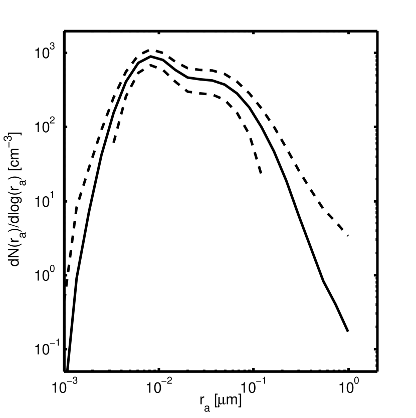
Figure 1: Averaged over the whole domain initial aerosol distribution. Dashed lines show standard deviation of the number for each aerosol bin.

An initial aerosol distribution in each computational grid was represented by 100 parcels. The aerosol spectrum used in the simulations is shown in figure 1. Aside from a spectrum averaged over the whole domain, the standard deviation of the values for each bin is also plotted. Variability in each bin is a result of a random sampling of the initial distribution with finite number of parcels. Although on average the spectrum agrees with an analytical distribution, sampling with a limited number of parcels leads to a variability of the distribution for a different grids and as a result it affects droplet number and size in each model grid during the condensational growth.

The model was forced by the surface temperature source prescribed as:

$$f_{t}(x,z)=A_{th}exp(-\frac{(x-x_{0})^{2}+(z-z_{0})^{2}}{800}),$$ (9)

with $A_{th}$=0.15 K/s and ($x_{0}$, $z_{0}$) set to (0,400). Simulations have been run for 1080s, with a time-step 0.25s. Microphysical grid in aerosol space (in ${\mu}m$) was specified as: $r_{a}(k)=10^{-3.2+k*0.2}$, with 30 bins. In radius space 28 bins were used, and radius for a bin $k$ was specified as: $r(k)=p^{1/3}r(k-1)$, with r(1)=1${\mu}m$ and $p$=2.

The following model setups are discussed in details in this article:

$REF$ - reference simulation. No representation of turbulence in eq. 3 (v^′=0). Deterministic flow velocity u^d at parcel location is determined by interpolating velocity from 4 (8 in 3D) nearest Eulerian computational grids to a parcel location. The vertical component of the parcel velocity is used to evaluate collision kernel.

$BIN$ - As far as parcel movement is concerned it is assumed that parcel velocity is equal to the air velocity interpolated to a parcel location, that is eq. 3 is not solved. The terminal velocity of the parcel is added to the vertical velocity. The parcel’s terminal velocity has been determined from the expression given by Simmel et al. (2002). To simplify calculations instead of the terminal velocity for a parcel size, terminal velocity for the center of the collision bin to which the parcel is assigned is used. When the collision kernel between parcels is calculated it is assumed that the parcel velocity is equal only to a terminal velocity. This setup mimics bin model as far as collision-coalescence process is concerned and assumes that turbulent transport and collision happen in different scales (are independent).

$TURB$ - for a given parcel deterministic flow velocity has 2 components deterministic: $u^{d}=u({\bf x})-\frac{1}{\rho}\frac{\partial}{\partial x_{i}}(\rho K_{l})$, where u(x) is Eulerian velocity for the computational grid to which parcel belongs, $K_{l}$ - diffusion coefficient for a Lagrangian model, and $\rho$ - gas density; and turbulent component v^′=$\sqrt{\frac{2K_{l}}{\triangle t}}$ with the derivation of of this model presented in the Appendix.

$REF2$ - Similar to $REF$, but in this case in additional to the difference in vertical velocity also difference in horizontal velocity is taken into account when evaluating the collision kernel.

3 Results

3.1 Evolution in space

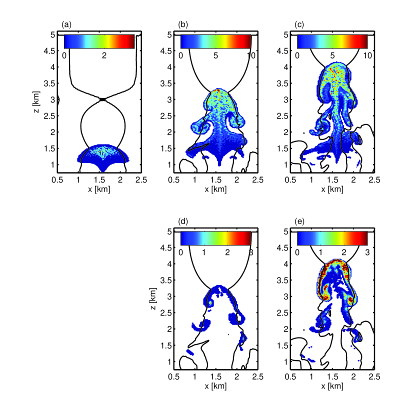
Figure 2: Upper row - cloud water mixing ratio (q_c) after 8 min. (a), 15 min (b) and 17 (c) min.; lower row - rain water mixing ratio (q_c) after 15 min. (d), 17 min (e) for a $REF$ run. Solid black line shows contour for value 0 of the vertical velocity.

Figure 2a-2c, shows snapshots of a cloud water mixing ratio ($q_{c}$) for the model solution for times 8 min. (fig. 2a), 15 min (fig. 2b) and 17 min (fig. 2c) for the $REF$ run. Cloud evolution exhibits features typically found in a 2D Cumulus developing in a stable stratified atmosphere and reported already by: Klaassen and Clark (1985), Grabowski and Clark (1991), Brenguier and Grabowski (1993). After reaching condensation level water vapor condenses and forms the cloud; air continues moving upward due to the temperature excess within the thermal. During the ascent in a stably stratified air cloud mixes with the environmental air, forming entrainment eddies. The cloud water mixing ratio reaches values as large as 12 g/m³ during the simulation, and at the end of the simulation the maximum vertical velocity is around 18 m/s. The cloud water mixing ratio shows relatively large variability in space, being a result of the fluctuations of the parcel number within the computational grid and also because of the variability in the randomly generated aerosol spectrum for each model grid.

Because in the numerical model the coalescence process is present, coalescence of the droplets in time leads to a drizzle formation. Figure 2d and 2e show evolution in time of the q_r - the rain water mixing ratio for a $REF$ case. A 50 ${\mu}m$ droplet radius is defined to be a border between a cloud and a rain droplet sizes. Large droplets reside near the edge of the cloud, and at the end of the simulation $q_{r}$ exceeds 3 g/kg. This behavior is typical for the three setups: $REF$, $TURB$ and $REF2$. For a $BIN$ case negligible q_r forms.

The edge of the cloud is a place where the difference in the vertical velocity within the collision grid is the largest (either because of the gradient of velocity between the interior and exterior of the cloud for $REF$ or $REF2$, or because TKE, used to derive stochastic velocity perturbations is largest). Additionally at the edge of the cloud the droplet spectrum can be broader than in the core of the cloud, which also enhances coalescence between droplets. The width of the droplet spectrum increases near the edge of the cloud because: a) the gradient of the supersaturation is largest there and as a result the interpolation of the thermodynamical parameters to a parcel location within the same computational grid different droplet populations may grow and evaporate at the same time depending on the distance from the edge of the cloud; b) vertical velocity changes sign near the cloud edge (in figure 2 the solid line shows a contour of the value 0), as a result droplets evaporate in a down-drafts near the cloud edge; and c) because largest droplets, formed in the center of the up-draft, after reaching cloud top start moving along cloud edge.

3.2 Evolution in time

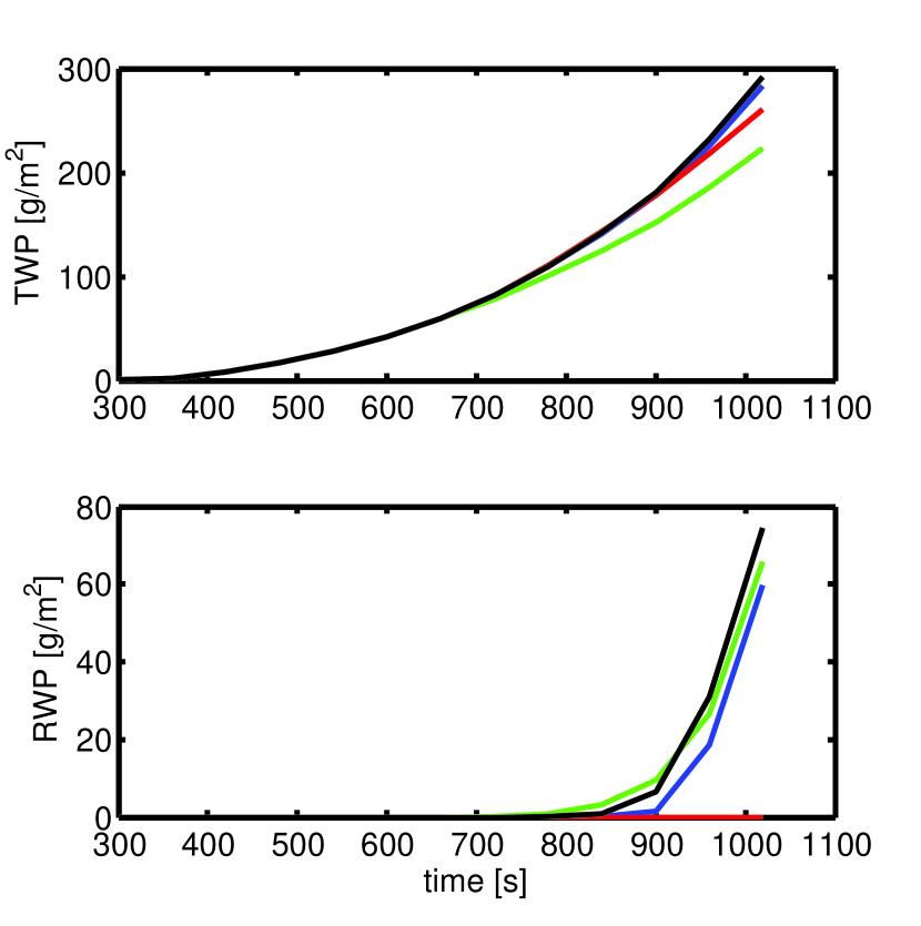
Figure 3: Evolution in time of a Total Water Path (a) and a Rain Water Path (b) for $REF$ - blue, $BIN$ - red, $TURB$ - green, $REF2$ - black.

Evolution of the TWP (Total Water Path) and RWP (Rain Water Path) in time for cases discussed are shown in figure 3. During the early stage of the cloud development TWP is very similar for all cases. In time, however, differences appear as a result of the interaction of the cloud and flow dynamics. The largest amount of water is for $REF2$ and $REF$ and smallest for $TURB$. The decrease in a TWP for a $TURB$ case can be associated with a random velocity of the air within the grid. As a result evaporation at the edge of the cloud may be larger for this case, because droplet trajectories can be different than for other three cases when velocity is interpolated to a parcel location. Much larger differences are observed for the RWP. The largest amount of water is for the $REF2$ case, the simulation where in coalescence calculation full velocity is taken into account. Compared to $REF$ simulation, $REF2$ has around 15% more RWP. For the $BIN$ simulation negligible amount of RWP has formed during the simulation time. But undoubtedly the coalescence process is active for this case also and droplets as large as 40 ${\mu}m$ have been formed in this simulation. These droplets are much smaller than for the three other simulations, where sizes up to 370 ${\mu}m$ are present.

3.3 Vertical profiles

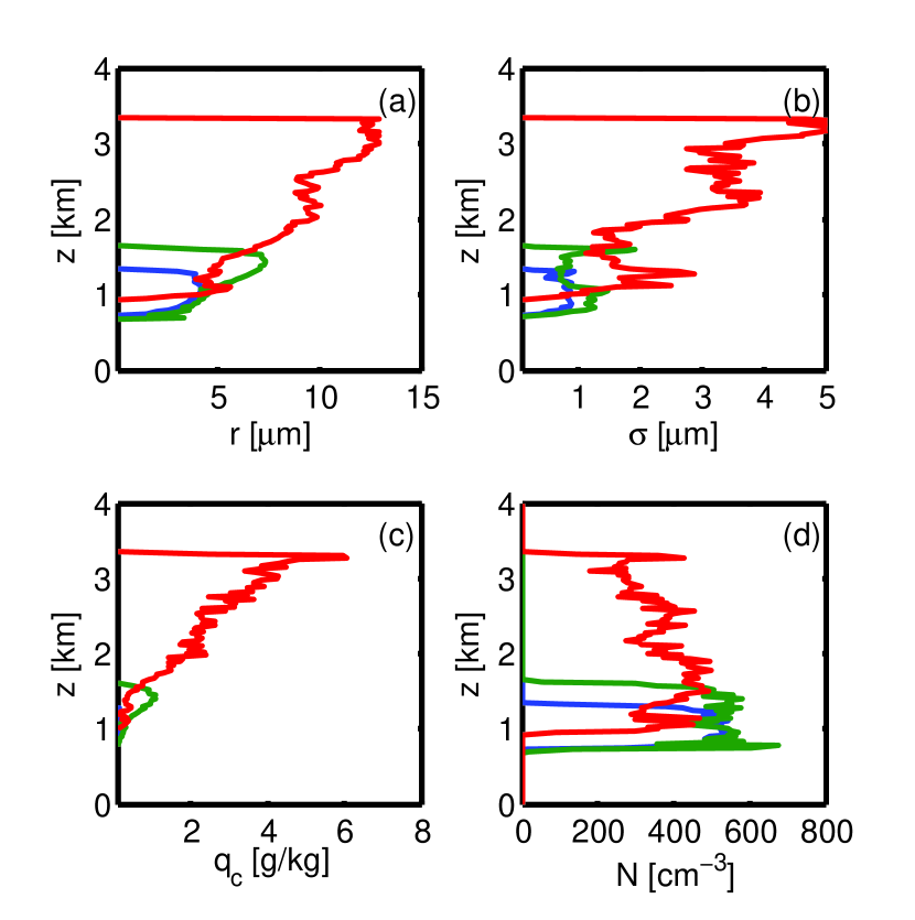
Figure 4: Vertical profiles for a $REF$ case of mean radius (a), standard deviation of the droplet spectrum on given level (b), q_c (c), and cloud droplet concentration (d) for times 6 min. - blue, 8 min. - green, 15 min. - red.

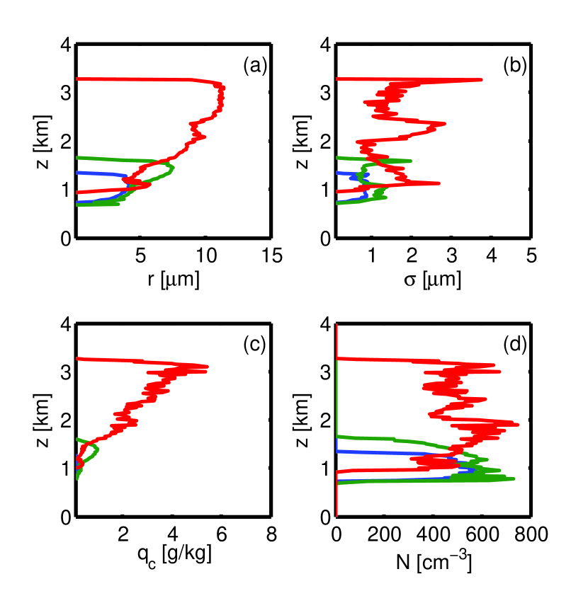
Figure 5: As figure 4, but for a $BIN$ case.

Vertical profiles of the mean radius ($r$), standard deviation of cloud droplet distribution ($\sigma$), cloud water mixing ratio ($qc$) and number of cloud droplets are shown in figures 4 for a $REF$ case (with very similar statistics observed for a $REF2$ and $TURB$ simulations) and for a $BIN$ case in figure 5 for a 3 times: 6, 8, and 15 minutes from the beginning of the simulation. These 3 times show cloud characteristics at the very early stage of the cloud development (the time when $q_{c}$ becomes larger than 0), through the initial formation of the drizzle (space distribution after 8 min. is shown in figures 2b and 2d), to the moment when significant drizzle develops (plots 2c and 2e). These diagnostics were calculated for each model level by taking into account only model grids, where $q_{c}$ was larger than 10^-3 g/kg. Figures 4 and 5 show a very similar development of the cloud for both cases. Initially a small amount of water condenses, but at the same time the mean radius is around 5 ${\mu}m$ and standard deviation around 1 ${\mu}m$. Around 1/3 of the total aerosol concentration activates at this stage. In time, the cloud thickens and after 8 minutes the cloud base moves upward. The mean droplet radius increases with height and reaches 12-13 ${\mu}m$ near the cloud top after 15 minutes At that time the number of cloud droplets decreases with height for a $REF$ case from 500 cm^-3 to 250 cm^-3. For the $BIN$ simulation, the cloud droplet concentration does not change significantly with height and oscillates around 500 cm^-3. Another difference between these 2 cases is in the standard deviation of the cloud droplet distribution after 15 min. above 2.5 km, and for the $BIN$ case standard deviation is around 1.5 ${\mu}m$, except at the cloud top, where it reaches 4.2 ${\mu}m$. For $REF$ case it is of the order of 3.5 ${\mu}m$, with the value near the cloud top of $\sim$5 ${\mu}m$. At earlier times and below 2.5 km standard deviation is very similar for both cases.

3.4 Droplet and aerosol spectra

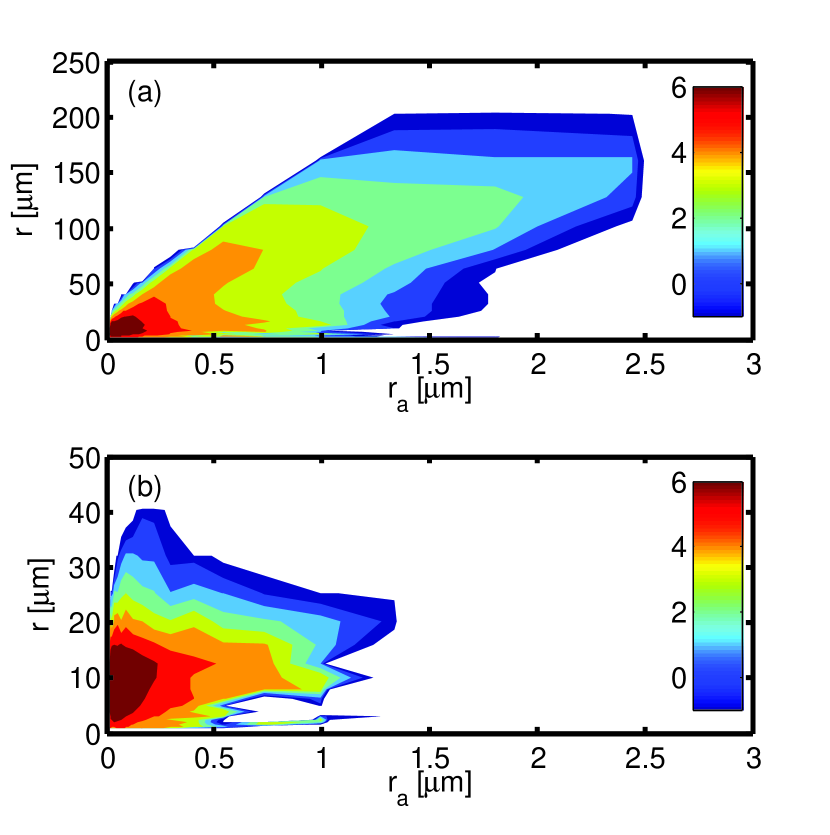
Figure 6: Relation between aerosol size and droplet size for grids with q${}_{c}>10^{-3}$ - Log₁₀(N(r,r_a)) for run $REF$ (a) and $BIN$ (b).

Because for each parcel information about droplet size and aerosol size is available, the relation between aerosol sizes and droplet sizes can be derived. Figure 6 shows this relation mapped on a Eulerian microphysical grid after 18 minutes. The relation between aerosol size and droplet size is complex and for a given aerosol size there is a broad range of droplet sizes formed on it. Because initially aerosol sizes were limited to 1 ${\mu}m$, sizes larger than that were created in a coalescence process. Much larger sizes of both aerosol and droplet are present for a $REF$ case, where the coalescence is more intensive.

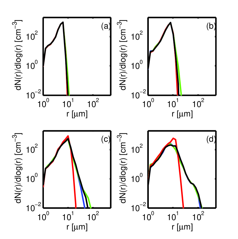
Figure 7: Droplet spectrum after 8 min. (a), 12 min. (b), 15 min (c) and 18 min (d) for a $REF$ - blue, $BIN$ - red, $TURB$ - green, $REF2$ - black.

From observations or spectrum resolving (bin) models typically information about either aerosol distribution or droplet distribution is derived. This information for microphysics in a Lagrangian framework is obtained by integrating relation shown in figure 6 along one of the dimensions. Averaged over the whole cloud the droplet spectrum is shown in figure 7. After 9 minutes - figure 7a the droplet spectrum is very similar for all cases. In time, similar to other cloud properties the differences between $BIN$ and $REF$, $TURB$ and $REF2$ emerge (7b, 7c, 7d). Formation of the large droplets for the $BIN$ simulation is much slower than for the remaining three cases. In an early stage of cloud development the largest droplets form for the $TURB$ case. At the end of the simulation, the spectra for $REF$, $TURB$ and $REF2$ cases are very similar.

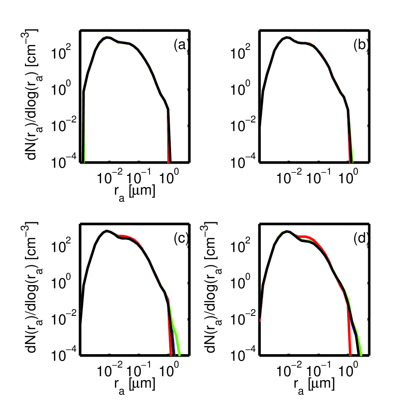
Figure 8: As figure 7 but for aerosol spectrum.

Evolution of an aerosol spectra averaged over the whole cloud is presented in figure 8. Because coalescence is processing not only droplet sizes, but also aerosol sizes, in time the aerosol spectrum also changes. There are indications, especially for later times, that aerosol is processed during droplet coalescence, but the differences between $BIN$ (where aerosol processing is negligible) and other three simulations are small. Fastest aerosol processing is for a $TURB$ simulations, with a smaller, for a $REF$ and $REF2$. Much more time is needed for the coalescence to process aerosol and form large/giant aerosol than the length of an idealized simulation discussed in this article. There is, however, evidence that this aerosol processing (eg. Twohy et al. (2013)) may be an important source of large aerosol, because within the $\sim$20 minutes maximum aerosol size has doubled, reaching 2.5 ${\mu}m$ radius (see fig. 6a) compared to 1 ${\mu}m$ initially. The increase of the concentration of the large aerosol is at the expense of the aerosol having sizes between 0.01 and 0.2 ${\mu}m$.

3.5 Velocity enhancement

The collision kernel, describing the probability of the coalescence of two colliding droplets can be written as:

$$K(r_{i},r_{j},v_{i},v_{j})=\pi(r_{i}+r_{j})^{2}|v_{i}-v_{j}|E_{i,j},$$ (10)

where r_i,r_j is the radius of a droplet $i$/$j$ with the corresponding velocity v_i/v_j, E_i,j is the gravitational collision efficiency. With the equation of motion solved for each parcel in the model, diagnostics of the relative velocity of colliding droplets can be determined. Equation 10 can be rewritten in the following way:

$$K(r_{i},r_{j},v_{i},v_{j})=\pi(r_{i}+r_{j})^{2}\frac{|v_{i}-v_{j}|}{|w_{i}-w_{j}|}|w_{i}-w_{j}|E_{i,j},$$ (11)

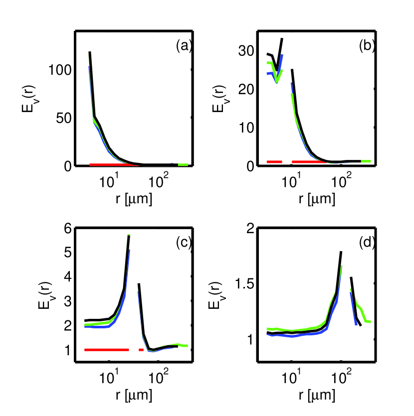
Figure 9: A velocity enhancement factor (E_v)for a different microphysical bins: bin 4 (a), bin 10 (b), bin 16 (c), bin 22 (d) for a $REF$ - blue, $BIN$ - red, $TURB$ - green, $REF2$ - black.

with the w_i/w_j being the terminal velocity for a parcel $i/j$. An enhancement of the gravitational collision efficiency due to the turbulent velocity fluctuations can be defined as: $E_{v}=<\frac{|v_{1}-v_{2}|}{|w_{1}-w_{2}|}>_{b}$, where $v_{i}$/$v_{j}$ is the velocity of colliding parcels, either vertical only or vertical and horizontal for a $REF2$, and $<>_{b}$ - averaging operator. Although it is possible to calculate this enhancement for each pair of droplets it is easier to use a bin structure the same as was used to map collisions between parcels, and in such a case $w_{i}$/$w_{j}$ represent a terminal velocity for the center of the bin rather than for an individual parcel, and averaging is done for each bin. Figure 9 shows a enhancement of the gravitational collision efficiency. Four panels show $E_{v}$ for a different bin sizes: 2.6 ${\mu}m$ (microphysical bin 4) - figure 9a, 9.1 ${\mu}m$ (microphysical bin 10) - figure 9b, 28.8${\mu}m$ (microphysical bin 16) - figure 9c, 94.3 ${\mu}m$ (microphysical bin 22) - figure 9d. The largest enhancement is for small bins with a value reaching 125 for a $TURB$ simulation. Simulation $REF2$ has value 120 and REF almost 105. Expectedly, the $BIN$ simulation has a constant value of $E_{v}$ - 1 independent on size, because the vertical velocity in this case is a droplet terminal velocity. With the increasing droplets sizes the departures of enhancement factor from 1 is smaller, and for bin 22 figure 10d it approaches 2. For a given bin, the largest $E_{v}$ is found for adjacent bins. For bins separated by a large distance $E_{v}$ is much smaller. The distribution of the $E_{v}$ is non-symmetric, with larger values of $E_{v}$ found for the sizes smaller than bin under consideration. The results presented in figure 9 show that even small differences in air velocity can affect velocity statistics for droplets having similar sizes and as a result moving with a similar velocities. For droplets having large differences in sizes turbulent velocity would have to be significantly larger than terminal velocity of larger droplets to influence $E_{v}$, which is not a case in the simulations discussed in this article. The large values of the enhancement of the gravitational collision efficiency for small droplets are assiciated with the fact that those droplets adjust quickly to the environmental flow, and as a result the velocity of small droplets is very similar to the velocity of the air. Much smaller values of the enhancement of the gravitational collision efficiency for large droplets are because these droplets need more time to adjust to the environmental flow and their terminal velocity is of the same order as air velocity fluctuations.

Diagnostics show that the maximum turbulent velocity for a $TURB$ case is around 3 m/s and has the same order as a terminal velocity of the 650 ${\mu}m$ droplet - $\sim$2.5 m/s. Note, however, that 3 m/s represents the largest value and standard deviation of the turbulent velocity for the whole cloud is $\sim$0.1-0.25 m/s. An example of the velocity fluctuations for run $REF$ and $TURB$ are shown in figure 10. There is a significant difference between the statistics for these two cases. For a $TURB$ case distribution of $u^{{}^{\prime}}$ and $w^{{}^{\prime}}$ are almost identical. For the $REF$ case anisotropy of the velocity fluctuations is observed, and tails for a $w^{{}^{\prime}}$ distribution is much broader than for a $u^{{}^{\prime}}$, with the statistics for $TURB$ case laying in-between $u^{{}^{\prime}}$ and $w^{{}^{\prime}}$ for a $REF$.

4 Conclusions

In this article two possible representation of the air turbulent velocity in a numerical model with a Lagrangian representation of microphysics are discussed. Air turbulent velocity in the model is represented either as a random walk process, with the standard deviation of velocity fluctuations derived from the diffusion coefficient predicted by the numerical model (Eulerian part) or as an interpolation of an air velocity to a parcel location. The random walk model is derived for an anelastic approximation and it’s shown that an additional, deterministic, term $1/{\rho}\nabla(\rho K_{m})$ needs to be included in a random walk model for consistency with the Eulerian model. It is argued that the mixing length used in a Lagrangian model should be smaller than used to derived diffusion coefficient for an Eulerian model; and the mixing length scale based on TKE and model time-step for use in Lagrangian microphysics is introduced. It is demonstrated that interpolation of the velocity to parcel location and use of this velocity in a collision kernel has a similar effect to representation of the turbulence as a random walk, and can be treated as an alternative to a random walk model. Additionally, for turbulence treated as a random walk, because all parcels within the particular computational grid have the same value of the deterministic velocity, fluctuations in the parcel number in a computational grid may be larger than for the case when velocity is interpolated to a parcel location. Unlike the random walk model, interpolation takes into account possible anisotropy in the flow velocity, also observed in a laboratory studies Malinowski et al. (2008), Korczyk et al. (2012) but in a much smaller scale.

If the sub-grid scale transport and droplet collisions occur on the same scale, air turbulent velocity can significantly enhance velocity differences between droplets, especially those having small sizes, when the turbulent velocity is much larger than terminal velocity of these droplets. In the cases discussed in this article enhancement as large as 120 has been observed for the case when only vertical velocity is taken into account when calculating relative velocity of colliding parcels. Allowing for the differences in a horizontal velocity $E_{v}$ increases by $\sim$15 %. The turbulent enhancement of the velocity of the colliding droplets obtained in this article is much larger than obtained form a DNS simulations and used in LES model by Wyszogrodzki et al. (2013) or Benmoshe et al. (2012). This difference is associated with the fact that in Lagrangian microphysics the same velocity is used for the transport and when evaluating collision kernel. The values obtained with air turbulent velocity fluctuations ($REF$, $TURB$) provide an upper limit of the impact of the air velocity fluctuations on gravitational collision efficiency, with the lower limit given by values from the BIN simulation. An additional parameterization is needed to accont for scale separation between transport and droplet interactions.

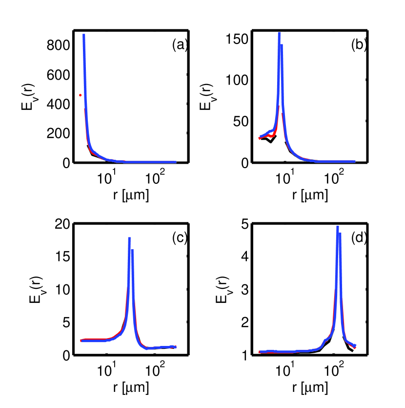
Figure 11: A velocity enhancement factor (E_v) for a different microphysical grids: for radius 2.6 ${\mu}m$ panel a, 9.1 ${\mu}m$ - panel b, 28.8${\mu}m$ - panel c, 94.3 ${\mu}m$ - panel d, for simulation: $REF2$ - black, $REF2$ with 55 bins used to represent droplet domain - red, $REF2$ with 109 bins used to represent droplet domain - blue.

Velocity enhancement diagnosed from the model is non-symmetric, with larger values for sizes smaller than size under consideration. The asymmetry, however, may be related to the microphysical grid, because in E_v averaged within a bin parcel velocity difference is normalized by a difference in the terminal velocity for bins these parcels belong to. As a result of the averaging and normalization E_v also depends on the number of bins used to represent domain in a radius space. Figure 11 shows E_v for a $REF$ case together with an additional 2 simulations using the same setup, but one with 55 bins (p=2${}^{1}/2$), and other with 108 bins (p=2${}^{1}/4$). With the increasing number of bins E_v also increases, reaching the value of 900 when the smallest bin is under consideration. A E_v values approach 1 independent on resolution in a radius space when the differences in droplet sizes is large.

Turbulent velocity enhancement can affect significantly drizzle formation. Simulation $BIN$, where droplet vertical velocity has been set to a terminal velocity, based on the bin to which droplets belong produces negligible amount of rain water, and much smaller than for other simulations droplet sizes. Note, however, that even in this case droplets do collide forming larger ones.

For simulations including a representation of air turbulen velocity fluctuations, drizzle forms initially preferentially near the cloud edge, near the entrainment eddies or near the cloud top, and often in the areas where q_c is elevated. The edge of the cloud is a place where due to entrainment and mixing droplet spectrum is broader than in the center of the cloud and as a result coalescence between droplets is more efficient. Additionally, because of the gradient of the velocity near the cloud edge, the differences in the relative velocity of parcels there is large and this also enhances probability of droplet coalescence. Formation of the first drizzle near the cloud edge it a bin model with the representation of the effect of turbulence on droplet collision rate has been also reported recently by Benmoshe et al. (2012).

The cloud droplet spectrum is relatively broad (of the order of $\sim 1{\mu}m)$ from the onset of the cloud formation. This value is much larger than reported for parcel models in the past and large enough to trigger the coalescence process even for the case with a very high cloud droplet concentration. It’s acknowledged, however, that when the standard deviation for each computational grid is considered values smaller than 0.1 ${\mu}$m are observed, indicating that very narrow (comparable to a parcel model) droplet distributions also form within computational grids.

Coalescence does process aerosol, but the time scale of this process is longer than $\sim$20 minutes of cloud evolution discussed here. Processing by multiple clouds is needed for the boundary layer aerosol to change the shape of the aerosol distribution.

5 Appendix

Consider conservation equation for a scalar for an anelastic approximation:

$$\frac{\partial\rho C}{\partial t}=-\nabla(\rho vC)+\nabla(\rho K\nabla C),$$ (12)

where $C$ - is concentration, $\rho$ - gas density, $v$ - gas velocity, $K$ - diffusion coefficient (note that in general $K$ is a tensor, however, here it is assumed that this tensor has only diagonal values not equal to 0; K_i,j=${\delta}_{i,j}K$). This equation can be written as:

$$\frac{\partial\rho C}{\partial t}=-\nabla[\rho C(v+\frac{1}{\rho}\nabla(\rho K)]+\triangle(\rho KC).$$ (13)

This equation corresponds to the following Stochastic Differential Equation in Ito sense (see for instance: Salamon et al. (2006) or Spivakovskaya et al. (2007) for the case when $\rho$ is constant):

$$dX=(v+\frac{1}{\rho}\nabla(\rho K))dt+\sqrt{2K}dW(t),$$ (14)

where $dW(t)$ is a Wiener process. Integration of this equation gives:

$$\triangle X=\int_{0}^{\triangle t}(v+\frac{1}{\rho}\nabla(\rho K))dt+\int_{0}^{\triangle t}\sqrt{2K}dW(t),$$ (15)

or in numerical representation for i-th direction, assuming that $v$, $K$ and $\rho$ are constant during the time step:

$$\triangle X_{i}=(v_{i}(X_{i})+\frac{1}{\rho(X_{i})}\frac{\partial}{\partial x_{i}}(\rho(X_{i})K(X_{i}))\triangle t+\sqrt{2K\triangle t}G,$$ (16)

where $G$ is a random number having normal distribution. It follows that effectively turbulent diffusion corresponds to a random walk process with mean velocity having two components, first being the velocity from the numerical model, the other accounting for a change in the density and diffusivity in a non-homogeneous medium:

$$v_{e}=v_{i}(X_{i})+\frac{1}{\rho(X_{i})}\frac{\partial}{\partial x_{i}}(\rho(X_{i})K(X_{i}));$$ (17)

and a random component:

$$v_{r}=\sqrt{\frac{2K}{\triangle t}}.$$ (18)

To find $K$ in numerical model an assumption must be made about the mixing length $l$, $K\sim l\cdot TKE^{1/2}$. Typically it is assumed to be of the order of a grid length. Although in the Eulerian model this assumption is justified, because mixing within each model grid must be completed within the time-step, in a Lagrangian transport model, where the exact location of each parcel is known it’s not necessary true. For a Lagrangian model a different length scale can be used, for instance from model time-step and turbulent kinetic energy (TKE), which is a prognostic variable in a sub-grid scale model. The following length scale can be defined: $l_{L}$=${\triangle t}\sqrt{2TKE/3}$, which for a 2D case discussed in this article is equal to $l_{L}$=${\triangle t}\sqrt{TKE}$. It follows that

$$v_{r}\sim\sqrt{TKE}.$$ (19)

This length scale is used only in a Lagrangian model to calculate diffusion coefficient and next the standard deviation of the velocity fluctuations and mean deterministic velocity.

Diagnostic from the model indicate that the velocity associated with the variability in $K$ and $\rho$ is very small $\sim$1 mm/s, but this term is nevertheless kept in the model.

Figure 10: Distribution of the velocity fluctuations within the computational grid for a $REF$ (a) and a $TURB$ (b) case. Solid line $u^{{}^{\prime}}$, dashed line - $w^{{}^{\prime}}$.

References

- Ackerman et al. [1995] Ackerman, A., Toon, O., Hobbs, P., 1995. A model for particle microphysics, turbulent mixing, and radiative transfer in the stratocumulus-topped marine boundary layer and comparisons with measurements. J. Atmos. Sci. 52, 1204–1236.
- Andrejczuk et al. [2012] Andrejczuk, M., Gadian, A., Blyth, A., Nov. 2012. Stratocumulus over SouthEast Pacific: Idealized 2D simulations with the Lagrangian Cloud Model. ArXiv e-prints.
- Andrejczuk et al. [2010] Andrejczuk, M., Grabowski, W., Reisner, J., Gadian, A., 2010. Cloud-aerosol interactions for boundary-layer stratocumulus in the lagrangian cloud model. J. Geophys. Res. 115, D22214, doi:10.1029/2010JD014248.
- Andrejczuk et al. [2008] Andrejczuk, M., Reisner, J. M., Henson, B. F., Dubey, M., Jeffery, C. A., 2008. The potential impacts of pollution on a nondrizzling stratus deck: Does aerosol number matter more than type? J. Geophys. Res. 113, D19204, doi:10.1029/2007JD009445.
- Bartlett and Jonas [1972] Bartlett, J. . T., Jonas, P. R., 1972. On the dispersion of the sizes of droplets growing by condensation in turbulent clouds. Quart. J. Roy. Meteor. Soc. 98, 150–164.
- Beard and Ochs [1993] Beard, K. V., Ochs, H. T., 1993. Warm-rain initiation: An overview of microphysical mechanisms. J. Appl. Meteor. 32, 608–625.
- Benmoshe et al. [2012] Benmoshe, N., Pinsky, M., Pokrovsky, A., Khain, A., 2012. Turbulent effects on the microphysics and initiation of warm rain in deep convective clouds. J. Geophys. Res. 117, D06220.
- Bewley and Lasher-Trapp [2005] Bewley, J. L., Lasher-Trapp, S. G., 2005. Progress on predicting the breadth of droplet size distributions observed in small cumuli. J. Atmos. Sci. 68, 2921–2929.
- Blyth et al. [2013] Blyth, A. M., Lowenstein, J. H., Huang, Y., Cui, Z., Davies, S., Carslaw, K. S., 2013. The production of warm rain in shallow maritime cumulus clouds. Q.J.R. Meteorol. Soc. 139, 20–31.
- Bodenschatz et al. [2010] Bodenschatz, E., Malinowski, S. P., Shaw, R. A., Stratmann, F., 2010. Can we understand clouds without turbulence? Science 327, 970–971.
- Brenguier and Grabowski [1993] Brenguier, J.-L., Grabowski, W. W., 1993. Cumulus entrainment and cloud droplet spectra: A numerical model within a two-dimensional dynamical framework. J. Atmos. Sci. 50, 120–136.
- Brown et al. [1989] Brown, P. N., Byrne, G. D., Hindmarsh, A. C., 1989. Vode: A variable coefficient ode solver. SIAM J. Sci. Stat. Comput. 10, 1038–1051.
- Cooper et al. [1997] Cooper, W. A., Bruintjes, R. T., Mather, G. K., 1997. Calculations pertaining to hygroscopic seeding with flares. J. Appl. Meteor. 36, 1449–1469.
- De Almeida [1976] De Almeida, F. C., 1976. The collisional problem of cloud droplets moving in a turbulent environinent-part i: A method of solution. Journal of the Atmospheric Sciences 33 (8), 1571–1578.
- Deardorff [1973] Deardorff, J., 1973. The use of subgrid transport equations in a three-dimensional model of atmospheric turbulence. J. Fluids Eng 95, 429–438.
- Devenish et al. [2012] Devenish, B. J., Bartello, P., Brenguier, J., Collins, L. R., Grabowski, W. W., IJzermans, R. H. A., Malinowski, S. P., Reeks, M. W., Vassilicos, J. C., Wang, L.-P., Warhaft, Z., 2012. Droplet growth in warm turbulent clouds. Quarterly Journal of the Royal Meteorological Society 138 (667), 1401–1429.
- Feingold et al. [1994] Feingold, G., Stevens, B., Cotton, W., Walko, R., 1994. An explicit cloud microphysics/les model designed to simulate the twomey effect. Atmos. Res. 33, 207–233.
- Franklin et al. [2005] Franklin, C. N., Vaillancourt, P. A., Yau, M. K., Bartello, P., 2005. Collision rates of cloud droplets in turbulent flow. J. Atmos. Sci. 62, 2451–2466.
- Goke et al. [2007] Goke, S., Ochs, H. T., Rauber, R. M., 2007. Radar analysis of precipitation initiation in maritime versus continental clouds near the florida coast: Inferences concerning the role of ccn and giant n uclei. J. Atmos. Sci. 64, 3695–3707.
- Grabowski [1989] Grabowski, W. W., 1989. Numerical experiments on the dynamics of the cloud-environment interface: Small cumulus in a shear-free environment. J. Atmos. Sci. 46, 3513–3541.
- Grabowski and Clark [1991] Grabowski, W. W., Clark, T. L., 1991. Cloud-evironment interface instability: Rising thermal calculations in two spatial dimensions. J. Atmos. Sci. 48, 527–546.
- Grabowski and Wang [2013] Grabowski, W. W., Wang, L., 2013. Growth of cloud droplets in a turbulent environment. Annual Review of Fluid Mechanics 45, 293–324.
- Jonas [1996] Jonas, P., 1996. Turbulence and cloud microphysics. Atmospheric Research 40 (2–4), 283 – 306.
- Kao et al. [1999] Kao, C., Hang, Y., Reisner, J., Smith, W., 1999. Test of the volume-of-fluid method on marine boundary layer clouds. Mon. Wea. Rev. 128, 1960–1970.
- Kenzelbach [1990] Kenzelbach, W., 1990. Simulation of pollutant transport in groundwater with the random walk method. Proceedings of the Dresden Symposium. IAHS Publ. no. 173., 265–279.
- Khain et al. [2004] Khain, A. P., Pokrovsky, A., Pinsky, M., Seifert, A., Phillips, V., 2004. Simulation of effects of atmospheric aerosols on deep turbulent convective clouds using a spectral microphysics mixed-phase cumulus cloud model. part i: Model description and possible applications. J. Atmos. Sci. 61, 2963–2982.
- Klaassen and Clark [1985] Klaassen, G. P., Clark, T. L., 1985. Dynamics of the cloud-environment interface and entrainment in small cumuli: Two-dimensional simulations in the absence of ambient shear. J. Atmos. Sci. 42, 2621–2642.
- Kogan [1991] Kogan, Y., 1991. The simulation of a convective cloud in a 3-d model with explicit microphysics. part i: Model description and sensitivity experiments. J. Atmos. Sci. 48, 1160–1189.
- Korczyk et al. [2012] Korczyk, P. M., Kowalewski, T. A., Malinowski, S. P., 2012. Turbulent mixing of clouds with the environment: Small scale two phase evaporating flow investigated in a laboratory by particle image velocimetry. Physica D: Nonlinear Phenomena 241 (3), 288 – 296, special Issue on Small Scale Turbulence.
- Lasher-Trapp et al. [2005] Lasher-Trapp, S. G., Cooper, W. A., Blyth, A. M., 2005. Broadening of droplet size distributions from entrainment and mixing in a cumulus cloud. Quarterly Journal of the Royal Meteorological Society 131, 195–220.
- Leroy et al. [2009] Leroy, D., Wobrock, W., Flossmann, A. I., 2009. The role of boundary layer aerosol particles for the development of deep convective clouds: A high-resolution 3d model with detailed (bin) microphysics applied to crystal-face. Atmos. Res. 91, 62–78.
- Long [1974] Long, A. B., 1974. Solutions to the droplet collection equation for polynomial kernels. J. Atmos. Sci. 31, 1040–1052.
- Malinowski et al. [2008] Malinowski, S. P., Andrejczuk, M., Grabowski, W. W., Korczyk, P., Kowalewski, T. A., Smolarkiewicz, P. K., 2008. Laboratory and modeling studies of cloud–clear air interfacial mixing: anisotropy of small-scale turbulence due to evaporative cooling. New Journal of Physics 10 (7), 075020.
- Margolin et al. [1995] Margolin, L., Reisner, J., Smolarkiewicz, P., 1995. Application of the volume of fluid method to the advection-condensation problem. Mon. Wea. Rev. 125, 2265–2273.
- Margolin et al. [1999] Margolin, L., Smolarkiewicz, P., Sorbjan, Z., 1999. Large-eddy simulations of convective boundary layers using nonoscillatory differencing. Physica D 133, 390–397.
- Ovchinnikov and Easter [2010] Ovchinnikov, M., Easter, R. C., 2010. Modeling aerosol growth by aqueous chemistry in a non-precipitating stratiform cloud. J. Geophys. Res. 115, D14210.
- Pinsky and Khain [2002] Pinsky, M., Khain, A., 2002. Effects of in-cloud nucleation and turbulence on droplet spectrum formation in cumulus clouds. Q. J. R. Meteorol. Soc. 128, 1–33.
- Pinsky et al. [2006] Pinsky, M. B., Khain, A. P., Grits, B., Shapiro, M., 2006. Collisions of small drops in a turbulent flow. part iii: Relative droplet fluxes and swept volumes. J. Atmos. Sci. 63, 2123–2139.
- Prusa et al. [2008] Prusa, J. M., Smolarkiewicz, P. K., Wyszogrodzki, A. A., 2008. Eulag, a computational model for multiscale flows. Computers & Fluids 37 (9), 1193–1207.
- Riechelmann et al. [2012] Riechelmann, T., Noh, Y., Raasch, S., 2012. A new method for large-eddy simulations of clouds with lagrangian droplets including the effects of turbulent collision. New Journal of Physics 14 (6), 065008.
- Salamon et al. [2006] Salamon, P., Fernàez-Garcia, D., Gó-Hernáez, J. J., 2006. A review and numerical assessment of the random walk particle tracking method. Journal of Contaminant Hydrology 87 (3.4), 277 – 305.
- Shima et al. [2009] Shima, S., Kusano, K., Kawano, A., Sugiyama, T., Kawahara, S., 2009. The super-droplet method for the numerical simulation of clouds and precipitation: a particle-based and probabilistic microphysics model coupled with a non-hydrostatic model. Quart. J. Roy. Meteor. Soc. 135, 1307–1320.
- Simmel et al. [2002] Simmel, M., Trautmann, T., Tetzlaff, G., 2002. Numerical solution of the stochastic collection equation comparison of the linear discrete method with other methods. Atmos. Res. 61, 135–148.
- Smolarkiewicz [1983] Smolarkiewicz, P., 1983. A simple positive definite advection scheme with small implicit diffusion. Mon. Wea. Rev. 111, 479–486.
- Smolarkiewicz and Grabowski [1990] Smolarkiewicz, P. K., Grabowski, W. W., 1990. The multidimensional positive definite advection transport algorithm: nonoscillatory option. Journal of Computational Physics 86 (2), 355–375.
- Smolarkiewicz and Margolin [1997] Smolarkiewicz, P. K., Margolin, L. G., 1997. On forward-in-time differencing for fluids: An eulerian/semi-lagrangian nonhydrostatic model for stratified flows. Atmos. OceanSpecial 35, 127–152.
-
Solch and Karcher [2010]
Solch, I., Karcher, B., 2010. A large-eddy model for cirrus clouds with
explicit aerosol and ice microphysics and lagrangian ice particle tracking.
Quarterly Journal of the Royal Meteorological Society 136 (653), 2074–2093.
URL http://dx.doi.org/10.1002/qj.689 - Spivakovskaya et al. [2007] Spivakovskaya, D., Heemink, A. W., Deleersnijder, E., 2007. The backward Îto method for the lagrangian simulation of transport processes with large space variations of the diffusivity. Ocean Science 3 (4), 525–535.
- Srivastava [1989] Srivastava, R. C., 1989. Growth of cloud drops by condensation: A criticism of currently accepted theory and a new approach. J. Atmos. Sci. 46, 869–887.
-
Twohy et al. [2013]
Twohy, C. H., Anderson, J. R., Toohey, D. W., Andrejczuk, M., Adams, A., Lytle,
M., George, R. C., Wood, R., Saide, P., Spak, S., Zuidema, P., Leon, D.,
2013. Impacts of aerosol particles on the microphysical and radiative
properties of stratocumulus clouds over the southeast pacific ocean.
Atmospheric Chemistry and Physics 13 (5), 2541–2562.
URL http://www.atmos-chem-phys.net/13/2541/2013/ - Wang et al. [2006] Wang, L., Franklin, C. N., Ayala, O., Grabowski, W. W., 2006. Probability distributions of angle of approach and relative velocity for colliding droplets in a turbulent flow. J. Atmos. Sci. 63, 881–900.
- Warner [1969a] Warner, J., 1969a. The microstructure of cumulus cloud. part I. general features of the droplet spectrum. J. Atmos. Sci. 26, 1049–1059.
- Warner [1969b] Warner, J., 1969b. The microstructure of cumulus cloud. part II. the effect on droplet size distribution of cloud nucleus spectrum and updraft velocity. Quart. J. Roy. Meteor. Soc. 26, 1272–1282.
- Whitby [1978] Whitby, K. T., 1978. The physical characteristics of sulfur aerosols. Atmospheric Environment (1967) 12 (1–3), 135–159.
- Wilson and Sawford [1996] Wilson, J., Sawford, B., 1996. Review of lagrangian stochastic models for trajectories in the turbulent atmosphere. Boundary-Layer Meteorology 78, 191–210.
- Wyszogrodzki et al. [2013] Wyszogrodzki, A. A., Grabowski, W. W., Wang, L., Ayala, O., 2013. Turbulent collision-coalescence in maritime shallow convection. Atmos. Chem. Phys. Discuss. 13, 9217–9265.
- Yum and Hudson [2005] Yum, S. S., Hudson, J. G., 2005. Adiabatic predictions and observations of cloud droplet spectral broadness. Atmospheric Research 73 (3–4), 203–223.