The Elliptic Gaudin Model: a Numerical Study

Abstract

The elliptic Gaudin model describes completely anisotropic spin systems with long range interactions. The model was proven to be quantum integrable by Gaudin and latter the exact solution was found by means of the algebraic Bethe ansatz. In spite of the appealing properties of the model, it has not yet been applied to any physical problem. We here generalize the exact solution to systems with arbitrary spins, and study numerically the behavior of the Bethe roots for a system with three different spins. Then, we propose an integrable anisotropic central spin model that we study numerically for very large systems.

I introduction

In 1976 Michel Gaudin proposed three quantum integrable models for spin 1/2 chains with infinite range interactions Gaudin . Two of these models, the rational or XXX and the hyperbolic-trigonometric or XXZ models, were solved for the spectrum and eigenstates. However, the exact solution of the third integrable model, the Elliptic Gaudin Model (EGM) or XYZ model, had to wait till 1996 Sklyanin for a complete solution in terms of the Algebraic Bethe Ansatz (ABA). The Gaudin models played an important role in the development and testing of several methods in quantum integrable theory, like the functional Bethe ansatz and the separation of variables Skl2 ; Skl3 , the relation with the Knizhnik-Zamolodchikov equations Bab ; babujian and with the corresponding Wess-Zumino-Witten models WZW , the construction of Bäcklund transformations Zullo , etc. On a different perspective, the rational Gaudin model Amico ; Duk1 was linked to the exact solution of the reduced Bardeen-Cooper-Schriefer (BCS) Hamiltonian solved exactly by Richardson Rich1 and proved to be quantum integrable by Cambiaggio, Rivas and Saraceno CRS . Exploiting this link, several families of exactly solvable models called Richardson-Gaudin (RG) models were proposed Amico ; Duk1 . Since then, the rational RG model found important applications to different areas of quantum many-body physics including ultrasmall superconducting grains Delft ; Links1 , Tavis-Cummings models atom-mol ; Lerma , cold atomic gases Schuck ; Links2 ; BCS-BEC , quantum dots Bortz ; Fari and nuclear structure Cooper ; Heavy (for a review see Duk2 ; Ortiz ). More recently, the hyperbolic RG model was applied to describe p-wave pairing in 2D lattices Sierra ; Romb ; Stin and 1D Kitaev wires Kitaev . With less success, there have been attempts to apply the EGM to matter-radiation problems including counter-rotating terms Kundu ; Hikami . However, these integrable models lack of the radiative excitation term or lead to non-hermitian Hamiltonians. On a different respect, the EGM has been used to study the thermalization process of a spin chain with long range interactions in the transition from integrability to chaos Relano . None of these works attempted to find a numerical solution of the Bethe equations.

The aim of this paper is to survey and generalize the exact solution of EGM for arbitrary SU(2) spins systems, and to study numerically the properties of the exact solutions in different scenarios. We first introduce the model with the corresponding exact solution in Sec. II. We then discuss a simple model of three different spins in Sec. III for which we show how to solve the Bethe equations in order to obtain the complete set of eigenstates. Next, we move to a physically oriented problem, a new integrable anisotropic central spin model (ACSM), in Sec. IV. In Sec. V we solve exactly the ACSM for long chains, and we extrapolate the ground state energy to the large $N$ limit, showing that it coincides with the classical spin approximation in the thermodynamic limit.

II The Elliptic Gaudin Model

The EGM was first proposed by GaudinGaudin as a particular family of integrable spin Hamiltonians with a fully anisotropic spin-spin interactions. The $N$ commuting integrals of motion for a system of $N$ arbitrary spins $S_{i}^{\alpha}$, with $\alpha=x,y,z$ and $i=1,\cdots,N$ are

$$R_{i}=\sum_{{j=1\atop(j\neq i)}}^{N}J_{ij}^{x}S_{i}^{x}S_{j}^{x}+J_{ij}^{y}S_{i}^{y}S_{j}^{y}+J_{ij}^{z}S_{i}^{z}S_{j}^{z},$$ (1)

where the matrices $J_{ij}^{\alpha}$ satisfy the Bethe equations

$$J_{ij}^{\alpha}J_{jk}^{\gamma}+J_{ji}^{\beta}J_{ik}^{\gamma}+J_{ik}^{\alpha}J_{kj}^{\beta} = 0,$$

in order to fulfill the integrability conditions $\left[R_{i},R_{j}\right]$=0.

Following Ref. babujian , the $J_{ij}^{\alpha}$ can be expressed in terms of the doubly periodic elliptic Jacobi functions of modulus $k$, $\operatorname{sn}(z,k)$, $\operatorname{cn}(z,k)$ and $\operatorname{dn}(z,k)$ (for brevity, in general, we will not explicitly write the modulus), and a set of $N$ arbitrary coefficients $z_{i}$ as

$$J_{ij}^{x}=\frac{1+k\leavevmode\nobreak\ \operatorname{sn}^{2}(z_{i}-z_{j})}{\operatorname{sn}(z_{i}-z_{j})},$$

$$J_{ij}^{y}=\frac{1-k\leavevmode\nobreak\ \operatorname{sn}^{2}(z_{i}-z_{j})}{\operatorname{sn}(z_{i}-z_{j})},$$ (2)

$$J_{ij}^{z}=\frac{\leavevmode\nobreak\ \operatorname{cn}(z_{i}-z_{j})\,\operatorname{dn}(z_{i}-z_{j})}{\operatorname{sn}(z_{i}-z_{j})}.$$

Alternatively, the integrals of motion $R_{i}$ can be expressed in terms of the raising and lowering spin operators $S^{\pm}=S^{x}\pm iS^{y}$ as

$$R_{i} =\sum_{j\left(\neq i\right)}\left[\frac{k}{2}\leavevmode\nobreak\ \operatorname{sn}(z_{i}-z_{j})\leavevmode\nobreak\ \left(S_{i}^{+}S_{j}^{+}+S_{i}^{-}S_{j}^{-}\right)+\frac{1}{2\operatorname{sn}(z_{i}-z_{j})}\left(S_{i}^{+}S_{j}^{-}+S_{i}^{-}S_{j}^{+}\right)\right.$$

$$\left.+\frac{\leavevmode\nobreak\ \operatorname{cn}(z_{i}-z_{j})\operatorname{dn}(z_{i}-z_{j})}{\operatorname{sn}(z_{i}-z_{j})}S_{i}^{z}S_{j}^{z}\right].$$ (3)

The elliptic integrals of motion break the $su(2)$ symmetry associated with the conservation of the total spin $S$ and the $u(1)$ symmetry associated with the conservation of the $z$ component of the total spin $S^{z}$. However, the model preserves a discrete $Z_{2}$ symmetry associated with a $\pi$ rotation of every spin around an arbitrary axis. Assuming $z$ as the quantization axis, a rotation by an angle $\pi$ around this axis is related to the parity operator $P=\prod_{i=1}^{N}e^{i\pi\left(S_{i}^{z}+s_{i}\right)}$ with eigenvalues $+1$ for positive parity and $-1$ for negative parity. Therefore, the complete set of common eigenstates of the integrals of motion can be classified in two subsets of even or odd parity.

The exact solution comprising the eigenvalues of the integrals of motion and the equations for determining the spectral parameters for a system of $N$ spins with $s_{i}=\frac{1}{2}$ has been obtained by means of the ABA in references Sklyanin ; babujian . Here, we present the exact solution for a general system of $N$ arbitrary spins $s_{i}$. The derivation starting from a system of 1/2 spins is given in the Appendix. The eigenvalues $r_{i}$ of the integrals of motion (1), depending on a set of $M$ roots $\lambda_{\alpha}$ to be determined by the Bethe equations that will be introduced below, are:

$$r_{i}=s_{i}\left[\sum_{j(\neq i)}^{N}\,s_{j}\,\left(\varphi_{4}(z_{i}-z_{j})+\varphi_{1}(z_{i}-z_{j})\right)-\sum_{\alpha=1}^{M}\left(\varphi_{4}(z_{i}-\lambda_{\alpha})+\varphi_{1}(z_{i}-\lambda_{\alpha})\right)+i\frac{\pi l}{2K}\right],$$ (4)

where $M=\sum_{i=1}^{N}s_{i}$. Any combination of spins $s_{i}$ is allowed as long as the resulting summation $M$ is integer. Notice that $M=N/2$ for the $s_{i}=1/2$ spin case and therefore, it would only admit an exact solution for an even number of spins $N$. In addition, $l$ is an integer number that can take the values 0 or 1 in order to identify the two parity sectors.

At this point, we have to introduce the Jacobi Theta functions Abramowitz ; NIST $\Theta(u,k)=\vartheta_{4}\left(v|q\right)$ and $\mathrm{H}(u,k)=\vartheta_{1}\left(v|q\right)$, with the variable transformation $v=\frac{\pi u}{2K}$. In these definitions $K(k)=\int_{0}^{\pi/2}\frac{d\theta}{\sqrt{1-k^{2}\sin^{2}\theta}}$ is the complete elliptic integral of the first kind, $K^{\prime}(k)=K\left(\sqrt{1-k^{2}}\right)$ and the nome $q=e^{-\pi K^{\prime}/K}$. The functions $\varphi_{1}(u)$, and $\varphi_{4}(u)$ can be defined now following Gould , as :

$$\varphi_{1}(u)=\frac{H^{\prime}(u)}{H(u)}\,,\qquad\qquad\varphi_{4}=\frac{\Theta^{\prime}(u)}{\Theta(u)}\;.$$

The $M$ roots $\lambda_{\alpha}$ in eq (4) are determined by solving the set of $M$ coupled Bethe equations (see the Appendix):

$$\sum_{j=1}^{N}\,s_{j}\,\left(\varphi_{4}(\lambda_{\alpha}-z_{j})+\varphi_{1}(\lambda_{\alpha}-z_{j})\right)-\sum_{\beta(\neq\alpha)}^{M}\left(\varphi_{4}(\lambda_{\alpha}-\lambda_{\beta})+\varphi_{1}(\lambda_{\alpha}-\lambda_{\beta})\right)+i\frac{\pi l}{2K} =0\,.$$ (5)

The function $\varphi(\lambda)=\varphi_{1}(\lambda)+\varphi_{4}(\lambda)$ appearing in the eigenvalues (4) and in the Bethe equations (5) has the special property of being periodic in the real part of its argument but “quasi periodic” in the imaginary part, i.e. $\varphi(\lambda+i\,K^{\prime})=\varphi(\lambda)+i\,C(k)$, where $K^{\prime}$ is the quasi-period (in the imaginary direction) and $C(k)$ is a real constant only depending on the elliptic modulus $k$. As a consequence the imaginary part of the Bethe roots are constrained to its natural interval $\mathrm{Im}(\lambda)\in[-\frac{K^{\prime}}{2},\frac{K^{\prime}}{2}]$. Numerical solutions obtained outside of this interval may lead to spurious non-physical results. On the other hand, as the real period of $\varphi(\lambda)$ is $2K$, the Bethe roots of any physical solution should be constraint to the fundamental rectangle of the complex plain given by $[0,2K]\times[-\frac{K^{\prime}}{2},\frac{K^{\prime}}{2}]$ .

We next analyze the behavior of the integrals $R_{i}$ in the two limits $k\to 0$ and $k\to 1$. Taking into account that for $k\to 0$, $\operatorname{sn}\left(u,k\right)\to\sin\left(u\right)$, $\operatorname{cn}\left(u,k\right)\to\cos\left(u\right)$ and $\operatorname{dn}\left(u,k\right)\to 1$, it is easy to check that the elliptic integrals $R_{i}$ (3) transform into the trigonometric ones:

$$R_{i}^{0}=\sum_{j\left(\neq i\right)}\left[\frac{1}{2\sin(z_{i}-z_{j})}\left(S_{i}^{+}S_{j}^{-}+S_{i}^{-}S_{j}^{+}\right)+\cot(z_{i}-z_{j})\,S_{i}^{z}S_{j}^{z}\right].$$

On the other hand, starting from the $x,y,z$ representation (1) and taking the limit $k\to 1$, the elliptic functions transform according to $\operatorname{sn}\left(u,k\right)\to\tanh\left(u\right)$ and $\operatorname{cn}\left(u,m\right),\,\operatorname{dn}(u,k)\,\to\>\mathrm{sech}\left(u\right)$, thus we obtain:

$$R_{i}^{1}=\sum_{j\left(\neq i\right)}\frac{1}{2\cosh(z_{i}-z_{j})\sinh(z_{i}-z_{j})}\left(S_{i}^{y}S_{j}^{y}+S_{i}^{z}S_{j}^{z}\right)+\frac{\cosh^{2}(z_{i}-z_{j})+\sinh^{2}(z_{i}-z_{j})}{\cosh(z_{i}-z_{j})\sinh(z_{i}-z_{j})}S_{i}^{x}S_{j}^{x}.$$

Performing a cyclic permutation of the axis and making use of some identities of the hyperbolic functions, we finally obtain the Gaudin hyperbolic integrals:

$$R_{i}^{1}=\sum_{j\left(\neq i\right)}\left[\frac{1}{2\sinh(\eta_{i}-\eta_{j})}\left(S_{i}^{+}S_{j}^{-}+S_{i}^{-}S_{j}^{+}\right)+\coth(\eta_{i}-\eta_{j})\,S_{i}^{z}S_{j}^{z}\right],$$

where $\eta_{i}=2\,z_{i}$.

In a similar way, it can be shown that the eigenvalues (4) and Bethe equations (5), reduce to the corresponding trigonometric and hyperbolic Gaudin solutions.

III A three-spin system

In order to understand the behavior of the Bethe roots for the different eigenstates we treat in this section the simplest integrable EGM with three different spins, $N=3$, and $s_{1}=1/2$, $s_{2}=1$, $s_{3}=3/2$. We construct an exactly solvable spin Hamiltonian as a linear combination of the integrals of motion

$$H=\sum_{i<j}^{3}\sum_{\alpha=1}^{3}H_{ij}^{\alpha}S_{i}^{\alpha}S_{j}^{\alpha}\,,$$ (6)

We choose for the Hamiltonian $H=-\frac{1}{2}R_{1}-\frac{1}{4}R_{2}$, with the parameters $z_{i}=0,\,0.2,\,0.4$ and the elliptic modulus $k=\frac{1}{2}$. The corresponding coefficients $H_{ij}^{\alpha}$ are displayed in Table 1.

$H_{12}^{x}$	$H_{12}^{y}$	$H_{12}^{z}$	$H_{13}^{x}$	$H_{13}^{y}$	$H_{13}^{z}$	$H_{23}^{x}$	$H_{23}^{y}$	$H_{23}^{z}$
1.28522	1.23563	1.2293	1.38861	1.19509	1.16865	1.28522	1.23563	1.2293

Table 1: Exchange couplings of the three-spin Hamiltonian (6).

The dimension of the Hilbert space is $d=\prod_{i=1}^{3}\left(2s_{i}+1\right)=24$. The Hamiltonian matrix is block diagonal with $d_{+}=12$ for positive parity and $d_{-}=12$ for negative parity. The number of Bethe equations (5) and roots is $M=\sum_{i=1}^{3}s_{i}=3$. For each parity sector, defined by $l=0$ or $1$, we look for 12 different solutions with the three roots restricted to the fundamental rectangle defined by $0<\mathrm{Re}(\lambda)<2K$ and $-\frac{K^{\prime}}{2}\leq\mathrm{Im}(\lambda)\leq\frac{K^{\prime}}{2}$. For this particular case $2K=3.3715$ and $\frac{K^{\prime}}{2}=1.07826.$

Tables 2 and 3 depict the complete set of eigenvalues and the corresponding values of the Bethe roots for positive and negative parity respectively. For positive parity $\left(l=0\right)$ and real parameters $z_{i}$, the Bethe roots are real or complex conjugate pairs with the exception of roots having the imaginary part equal to half the imaginary quasi-period $\left(\pm\frac{K^{\prime}}{2}\right)$. In the latter case the pair of complex roots need not to be a conjugate pair (real parts could be different). Moreover, complex conjugation of all roots gives the same solution due to the quasi-periodicity of the Jacobian functions. On the other hand, for negative parity $\left(l=1\right)$ one of the roots is always complex with the imaginary part equal to half the imaginary quasi-period $\left(+\frac{K^{\prime}}{2}\right)$, to compensate the imaginary term added to the Bethe equations. The other roots could be real, or complex pairs following the same behavior as in the $l=0$ case.

As a final remark, we have checked that the eigenvalues obtained solving the Bethe equations (5) fully agree with the results of an exact diagonalization of the Hamiltonian $\left(\ref{ham3}\right)$.

$E$	$\lambda_{1}$	$\lambda_{2}$	$\lambda_{3}$
-8.13147	0.277673	0.261164 + 0.115827 i	0.261164 - 0.115827 i
-5.64950	0.0674548	0.268200	2.150100
-5.48168	1.92346	0.281146 + 0.0491301 i	0.281146 – 0.0491301 i
-0.850805	0.286691	0.726263 + 1.07826 i	3.15855 – 1.07826 i
-0.758290	0.286760	0.257994 + 1.07826 i	1.94100 – 1.07826 i
-0.649792	0.0448926	2.06330 + 0.519302 i	2.06330  – 0.519302 i
-0.615993	0.0473203	0.375176 + 1.07826 i	2.06325 – 1.07826 i
-0.606659	0.0481756	0.825910 – 1.07826 i	3.29741 + 1.07826 i
-0.394121	0.287018	1.94224 + 0.516064 i	1.94224 – 0.516064 i
6.69616	1.95117	0.612035 – 1.07826 i	3.29405 + 1.07826 i
6.88050	1.95157	0.268084 – 1.07826 i	1.95185 + 1.07826 i
7.22436	1.95228	1.95248 + 0.704049 i	1.95248 – 0.704049 i

Table 2: Eigenvalues and Bethe roots in the positive parity sector $(l=0)$ of the three-spin Hamiltonian (6).

$E$	$\lambda_{1}$	$\lambda_{2}$	$\lambda_{3}$
-5.86850	0.239016 + 1.07826 i	0.280492 + 0.0487235 i	0.280492 – 0.0487235 i
-5.64331	0.0682364	0.268316	2.14920 + 1.07826 i
-5.59109	0.0727121	0.269232	0.458056 + 1.07826 i
-5.52799	0.281070 + 0.0490841 i	0.281070 – 0.0490841 i	1.92361 + 1.07826 i
-0.714459	0.286793	1.94080	0.258161 + 1.07826 i
-0.649689	0.0448967	2.06348	2.06312 + 1.07826 i
-0.619842	0.0469765	2.06361	0.375167 + 1.07826 i
-0.395533	0.287017	1.94206	1.94243 + 1.07826 i
6.59546	0.267512 + 1.07826 i	0.985596 + 1.07826	2.91839 – 1.07826 i
6.64346	0.599786 + 1.07826 i	1.95133 – 1.07826 i	3.30613 + 1.07826 i
6.88448	0.268092 + 1.07826 i	1.95170 + 0.496275 i	1.95170 – 0.496275 i
7.22431	1.95235 + 0.345399 i	1.95235 – 0.345399 i	1.95255 +.07826 i

Table 3: Eigenvalues and Bethe roots in the negative parity sector $(l=1)$ of the three-spin Hamiltonian (6).

IV The Anisotropic Central Spin Model

The central spin model (CSM), describing the hyperfine interaction of an electron spin in a quantum dot with a non-interacting system of surrounding nuclear spins, has been proposed as the main component of spintronic devises and solid state qubits CSM-Rev . The isotropic CSM Hamiltonian with Heisenberg exchange couplings between the central spin and the nuclear spin bath, subjected to an external magnetic field, is precisely one of the integrals of motion of the rational RG model. As such, it has been extensively studied using exact solutions Bortz ; Fari . Anisotropic effects due to the hyperfine interaction between the central spin and the nuclear bath can still be investigated within the Hyperbolic or XXZ RG model Fisher . However, the inclusion of the quadrupole coupling in the electron-bath interaction goes beyond the XXZ model Sini . Here, as a physically oriented example of a quantum integrable system derived from the EGM, we study a modified anisotropic central spin model (ACSM) without an external magnetic field. The introduction of an external magnetic field breaks the integrability of the EGM since it does not admit linear terms as opposed to the rational and trigonometric-hyperbolic cases. In our model the system is composed by a single electronic spin $s_{1}=\frac{1}{2}$ interacting with the $N-1$ nuclear spins $\frac{1}{2}$ of the bath. The hyperfine and quadrupole couplings between the electron and the surrounding spins is described by a completely anisotropic antiferromagnetic exchange interaction. We assume that the electron spin is located at position $z_{1}=0$, while the environmental spins are uniformly distributed within a linear segment at a finite distance $a$ $\left(z_{2}=a\right)$ with the last spin at position $z_{N}=b$, with $0<a<b\leq K$. The restriction for $b$ to be lower than or equal to $K$ is necessary to keep the interaction decreasing with distance in the selected interval. Therefore, the values of the fixed parameters $z$ are given by $z_{i}=a+\frac{i-2}{N-2}(b-a)$ for $i>1$. The anisotropic central spin Hamiltonian is defined by the first integral of motion (1) of the EGM:

$$H_{ACSM}=-R_{1}=\sum_{j=2}^{N}\left(J_{j}^{x}S_{1}^{x}S_{j}^{x}+J_{j}^{y}S_{1}^{y}S_{j}^{y}+J_{j}^{z}S_{1}^{z}S_{j}^{z}\right)\,,$$ (7)

where $J_{j}^{\alpha}=-J_{1j}^{\alpha}(-z_{j})=J_{1j}^{\alpha}(z_{j})$ for $\alpha\equiv x,y,z$ as given in Eq. (2). The properties of elliptic functions determine the relation between the exchange interactions in the $x$, $y$, $z$ directions as $J_{j}^{x}>J_{j}^{y}>J_{j}^{z}$  for  $0<z_{j}<K$. Figure 1 shows the three components of the interaction as a function of distance for $k=0.5$. In the horizontal axis we display, as an example, a spin network with $N-1=7$ environmental spins uniformly distributed in a segment with $a=0.2$ and $b=0.6$.

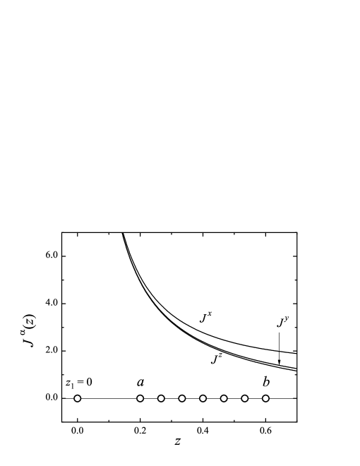
Figure 1: Exchange couplings of central spin Hamiltonian (7) as a function of distance. In the horizontal axis we show as an example a system with $N=8$ spins.

In order to gain insight into the structure of the GS wavefunction we explore the classical description of the model. In this approximation each spin $\frac{1}{2}$ operator is replaced by $S\equiv\frac{1}{2}[cos\varphi\,sin\theta,sin\varphi\,sin\theta,cos\theta]$, where $\theta$ and $\varphi$ are the usual polar and azimuthal angles satisfying $0\leq\theta\leq\pi$ and $0\leq\varphi\leq 2\pi$. Inserting into the Hamiltonian (7), the classical energy is given by

$$E_{cl}=\frac{1}{4}\sum_{j=2}^{N}\left(sin\theta_{1}\,sin\theta_{j}\left[J_{j}^{x}\,cos\varphi_{1}\,cos\varphi_{j}\,+J_{j}^{y}\,sin\varphi_{1}\,sin\varphi_{j}\right]+J_{j}^{z}\,cos\theta_{1}\,cos\theta_{j}\right)=\frac{1}{4}\,\sum_{j=2}^{N}\,E_{j}\,.$$ (8)

Our task is to find the absolute minimum of the classical energy $E_{cl}$ with respect to the angular variables of the central spin $\theta_{1}$, $\varphi_{1}$, and those of the nuclear spins $\{\theta_{j},\varphi_{j}\}_{j=2}^{N}$. Each term of the sum $E_{j}$ depends exclusively on the angles of a particular nuclear spin $j$ and the angles of the central spin. Minimization with respect to the angles leads to a system of $2\times N$ coupled variational equations. However, minimizing each term $E_{j}$ independently will yield the absolute minimum if each solution is compatible with a unique value of the central spin variables $\theta_{1},\varphi_{1}$. Notice that even though the spins in the bath are non-interacting, the latter condition induces an effective interaction through the central spin. By solving the four variational equations derived from the minimization of each $E_{j}$ we obtain different classes of solutions corresponding to stationary values of $E_{j}$ in the set $\{\pm J_{j}^{x},\,\pm J_{j}^{y},\,\pm J_{j}^{z}\}$. As the largest component of the interaction is $J_{j}^{x}$ we conclude that the minimum for each term is $E_{j}=-J_{j}^{x}$, and the corresponding angles are $\theta_{1}=\frac{\pi}{2}$, $\varphi_{1}=\pi$, $\theta_{j}=\frac{\pi}{2}$, $\varphi_{j}=0$ ($j>1)$. The classical GS corresponds to an antiferromagnetic state with all spins aligned into the $x$ axis, and the central spin pointing in the opposite direction to the environmental spins. Therefore, for the minimal energy configuration, the classical energy per spin is:

$$\frac{E_{cl}}{N}=-\frac{1}{4\,N}\,\sum_{j=2}^{N}\,J_{j}^{x}=-\frac{1}{4\,N}\,\sum_{j=2}^{N}\,\frac{1+k\leavevmode\nobreak\ \operatorname{sn}^{2}(z_{j})}{\operatorname{sn}(z_{j})}\;.$$ (9)

In order to find an expression for the classical energy density in the thermodynamic limit, i.e. $\lim_{N\to\infty}\frac{E_{cl}}{N}$, we define a normalized density distribution for the spins such that $\intop_{\Omega}\rho(z)\,dz=1$, where $\Omega\subset(0,K)$ is the compact interval containing all environmental spins (the parameters $z$’s except for $z_{1}$), so that the number of spins in an interval of length $dz$ is given by $(N-1)\,\rho(z)\,dz$. Introducing this distribution in equation (9) and taking the corresponding limit we obtain in general:

$$\mathcal{E}_{cl}=\lim_{N\to\infty}\,\frac{E_{cl}}{N}=-\frac{1}{4}\,\intop_{\Omega}\,\frac{1+k\leavevmode\nobreak\ \operatorname{sn}^{2}(z)}{\operatorname{sn}(z)}\,\rho(z)\,dz\,.$$ (10)

According to our model of equidistant bath spins, we assume a uniform distribution in the interval $\Omega=[a,\,b]$:

$$\rho(z)=\frac{1}{b-a}\;.$$ (11)

Finally, from Eq. (10) and making use of the uniform density (11) we obtain for the classical energy density in the thermodynamic limit:

$$\mathcal{E}_{cl}=\lim_{N\to\infty}\,\frac{E_{cl}}{N}=\frac{1}{4\left(a-b\right)}\,\intop_{\Omega}\,\frac{1+k\leavevmode\nobreak\ \operatorname{sn}^{2}(z)}{\operatorname{sn}(z)}\,dz,$$ (12)

which can be integrated to give

$$\mathcal{E}_{cl}=\frac{1}{4(a-b)}\,\log\left[\frac{\operatorname{sn}(b)\,\left(\operatorname{cn}(a)+\operatorname{dn}(a)\thinspace\right)\,(\operatorname{dn}(b)-k\,\operatorname{cn}(b)\,)}{\operatorname{sn}(a)\,\left(\operatorname{cn}(b)+\operatorname{dn}(b)\thinspace\right)\,(\operatorname{dn}(a)-k\,\operatorname{cn}(a)\,)}\right]\;.$$ (13)

We will later compare this classical energy density with the large $N$ limit of the exact solution.

V Exact solution of the ACSM

Let us now turn our attention to the exact quantum solution of the ACSM. We will analyze the distribution of spectral parameters or Bethe roots $\lambda_{\alpha}$ of the Bethe equations (5), as well as the ground state energy (per spin) of the Hamiltoninan $H_{ACSM}$, for several system sizes up to $N=300$. A large $N$ extrapolation of these results will allow us to compare with the classical energy density. We choose the modulus $k=0.5$, thus the fundamental interval is defined by $K(0.5)\approx 1.68575$. For the $z$’s interval we set $a=0.2$ and $b=0.6$.

Figure 2: Ground state Bethe roots of the ACSM (7) for different system sizes.

$N$	$\lambda_{1}N$	$\mathrm{Min(Re}(\lambda))$	$\mathrm{Max(Re}(\lambda))$	$\frac{E}{N}$
12	0.327300	2.120138	2.120487	-0.821616
20	0.329466	2.106036	2.106256	-0.792253
40	0.330390	2.095787	2.095898	-0.772954
80	0.330681	2.090745	2.090800	-0.7640486
100	0.330726	2.089743	2.089787	-0.762322
200	0.330805	2.087743	2.087765	-0.758920
300	0.330828	2.0870780	2.0870926	-0.757801
$\infty$	0.330869	2.0857505	2.0857505	-0.755586

Table 4: Extremum real values of the GS state Bethe roots and corresponding energies per spin for different $N$ values.

The numerical solution of the nonlinear system of equations (5) faces the usual problems of any Gaudin system, namely a huge number of independent solutions (the dimension of the system grows exponentially with $N$) and dangerous divergences which hinders numerical procedures based on iterative methods. Moreover, finding a specific solution strongly depends on the initial guess. To overcome these difficulties we first solve the system for a small number of spins, where we can identify the distribution of roots for the ground state as well as for all the excited states. We then follow a particular solution increasing $N$ by means of an algorithm described below.

In Fig. 2 we show the distribution of Bethe roots in the complex plane for the ground states ($l=0\mbox{)}$ of two systems, a small system with $N=12$ and large system with $N=300$. The complex plane is divided into three regions delimited by vertical lines crossing the real axes at $Re(\lambda)=0,\,a,\,b$ and $2K$. We found that the ground state has the root $\lambda_{1}$, which is associated with the central spin, always real and located in the first region satisfying $0<\lambda_{1}<a$, while the other roots are located over a smooth curve, symmetric with respect to the real axes, with $b<Re(\lambda)<2K$. We can see in Fig. 2, for $N=12$, that the five roots are almost vertically aligned at $Re(\lambda)\approx 2.120$. For $N=300$ the $149$ roots make up an almost vertical segment at $Re(\lambda)\approx 2.087$. The inset amplifies the third region adding several solutions for the intermediate systems with with $N=20,\,40$ and $100$. For increasing values of $N$ the real part of the roots in the arc decreases approaching a limiting value. Moreover, the first root $\lambda_{1}\to 0$ in this limit as can be seen in Table 4.

The ground state always displays the same pattern, with one real root in the first region $0<\lambda_{1}<a$ and $N-1$ roots distributed over a smooth arc in the third region, i.e. $Re(\lambda)>b$. A similar pattern takes place for the lowest energy state in the $l=1$ block. In Fig. 3 we show the distribution of Bethe roots for the GS (already displayed in Fig. 2) and the first three excited states in positive parity sector of the ACSM with 12 spins. As it can be seen, the arc of complex roots which characterizes the GS persists for the low lying excited states while some detached roots are distributed in other regions of the complex plane. Different distributions of the roots give rise to the complete set of eigenstates.

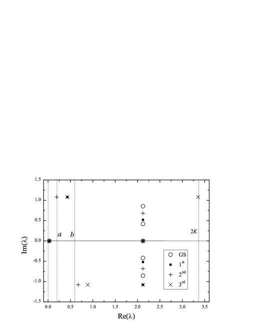
Figure 3: Bethe roots of the GS and first 3 excited states of the ACSM with N=12 spins.

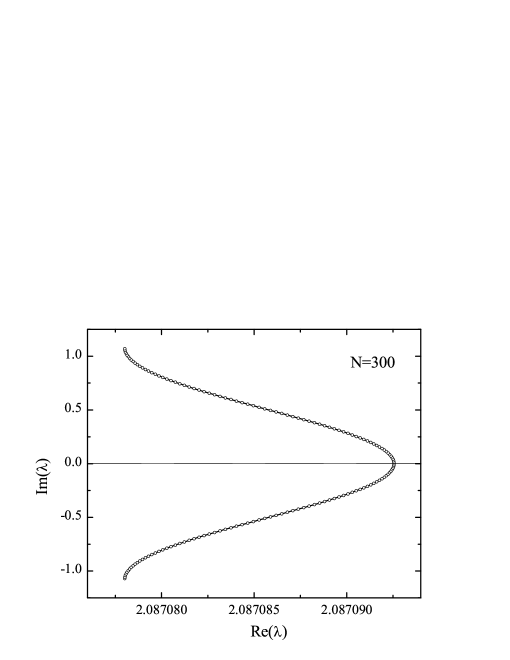
Figure 4: Ground state Bethe root of the ACSM (7) for $N=300$. The continuous line corresponds to the fit of Eq. (14).

The scale of the graph in figure 2, does not allow to appreciate the detailed form of the arcs in the third region. In figure 4 we show, with a smaller scale, the actual shape of the arc for $N=300$. The difference between the maximum and minimum real parts of the roots in the arc decreases with increasing $N$, becoming null at $N\to\infty$. Therefore, in the continuous limit the arc turns into a vertical segment with $\operatorname{Re}(\lambda)=2.08575$ with half of the quasi-periods as the interval extremes $-\frac{K^{\prime}}{2}\leq\operatorname{Im}\left(\lambda\right)\leq-\frac{K^{\prime}}{2}$ (see table 4).

In order to obtain the numerical ground state solution for a large $N$ system, we start from the solution of a small system. We then increase $N$, typically doubling it in each iteration. In each step we make a least square fit of the complex arc expressing the real part $\operatorname{Re}(\lambda)=x$ as a function of the imaginary part $\operatorname{Im}(\lambda)=y$ taken as the independent variable. An excellent agreement is obtained for any $N$ value by means of the 4-parameter function:

$$x=\alpha+\beta\,\operatorname{dn}(c_{1}\,y)\,\operatorname{cn}(c_{2}\,y)\;.$$ (14)

The continuous line in Fig. 4 corresponds to a fit of this function for the $N=300$ system. We take advantage of this excellent fit to generate, for each system of size $N$ the initial guess from the lower size system $N_{0}$. In addition, the initial guess for the first root $\lambda_{1}$ is obtained by a linear scaling $\lambda_{1}=\lambda_{1}^{0}\frac{N_{0}}{N}$. In both cases the index $0$ stands for the solution of the previous step. The procedure is stable, and it allows to find numerical solutions for very large systems.

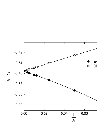
Figure 5: Exact quantum and classical GS energies per spin of the ACSM for different $N$ values. The extrapolated $N\to\infty$ limits coincide with the analytic value (13).

It is interesting to analyze the numerical results in the $N\to\infty$ limit. Table 4 shows these results for several values of $N$ and the numerical extrapolation to the thermodynamic limit. The fifth column of the table displays the energy per site and the extrapolated value in the thermodynamic limit. We can now compare these results with the classical energy density. For $a=0.2$, $b=0.6$ and $k=0.5$ equation (13) yields $\mathcal{E}_{cl}=-0.75558603$ showing an excellent agreement with the extrapolated result. In figure (5) we show a comparison between the classical energy (9) (open circles) and the quantum energy (black circles) for several values of $N$. Both branches converge to a common limit for $N\to\infty$. Continuous lines correspond to a third order polynomial least square fits. The gap between the classical and the quantum energies for finite systems is a direct consequence of the quantum fluctuations that disappear in the thermodynamic limit.

VI Summary

The rational and hyperbolic Gaudin models have been extensively employed lately to study many-body quantum systems in several branches of mesoscopic physics. On the contrary, the EGM derived by Gaudin in 1976 and solved exactly with the ABA in 1996 has been scarcely used as a mathematical tool to investigate many-body physical problems. In this article we have first summarized the integrals of motion of the model and the exact solution for systems with arbitrary spins. Subsequently, we discussed the behavior of the Bethe roots for the complete set of eigenstates of a system with three different spins. We showed that the Bethe roots should be restricted to the fundamental rectangle in order to warrant that every solution corresponds to a physical eigenstate. Finally, we introduced a particular anisotropic CSM, accounting for the hyperfine interaction of an electronic spin in a quantum dot with the environmental nuclear spins, and possible effects due to quadrupole couplings. The so called ACSM was solved exactly for large number of spins and the GS energy was extrapolated to the thermodynamic limit, which coincides with the classical approximation. We hope that our numerical studies would pave the way to applications of the EGM to other physical many-body systems.

Appendix. Generalization of the EGM to arbitrary spins

We start with the known integrals of motion, the corresponding eigenvalues and the Bethe equations for spin $1/2$ systems babujian

$$H_{a}=\sum_{b\left(\neq a\right)=1}^{\mathcal{N}}\left[J^{x}\left(z_{a}-z_{b}\right)\leavevmode\nobreak\ S_{a}^{x}S_{b}^{x}+J^{y}\left(z_{a}-z_{b}\right)\leavevmode\nobreak\ S_{a}^{y}S_{b}^{y}+J^{z}\left(z_{a}-z_{b}\right)\leavevmode\nobreak\ S_{a}^{z}S_{b}^{z}\right],$$ (15)

$$h_{a}=\frac{1}{4}\sum_{b\left(\neq a\right)=1}^{\mathcal{N}}\varphi\left(z_{a}-z_{b}\right)-\frac{1}{2}\sum_{\alpha=1}^{\mathcal{M}}\varphi\left(z_{a}-\lambda_{\alpha}\right)+\frac{i\pi l}{4K},$$ (16)

$$\frac{1}{2}\sum_{a=1}^{\mathcal{N}}\varphi\left(\lambda_{\alpha}-z_{a}\right)-\sum_{\beta\left(\neq\alpha\right)=1}^{\mathcal{M}}\varphi\left(\lambda_{\alpha}-\lambda_{\beta}\right)+\frac{i\pi l}{2K}=0,$$ (17)

where $\mathcal{N}$ is the number of spins and $\mathcal{M}=\mathcal{N}/2$ the number of roots.

Following Ref. Gaudin we now group an arbitrary number of adjacent spins into clusters and define a new lattice with sites $i$ and spins $S_{i}=\sum_{a=a_{i}}^{a_{i}+n_{i}}S_{a}$, where $a_{i}$ is leftmost site of the cluster $i$ and $n_{i}$ the number of spins in the cluster. The new lattice fulfills $\mathcal{N}=\sum_{i=1}^{N}n_{i}$, where $N$ is the number of clusters or sites in the new lattice. We recall that the functions $J\left(x\right)$ and $\varphi\left(x\right)$ are odd functions. The new integrals of motion are

$$R_{i} =\sum_{a=a_{i}}^{a_{i}+n_{i}}H_{a}=\sum_{a=a_{i}}^{a_{i}+n_{i}}\sum_{b\left(\neq a\right)=a_{i}}^{a_{i}+n_{i}}\left[J^{x}\left(z_{a}-z_{b}\right)\leavevmode\nobreak\ S_{a}^{x}S_{b}^{x}+J^{y}\left(z_{a}-z_{b}\right)\leavevmode\nobreak\ S_{a}^{y}S_{b}^{y}+J^{z}\left(z_{a}-z_{b}\right)\leavevmode\nobreak\ S_{a}^{z}S_{b}^{z}\right]+$$

$$\sum_{a=a_{i}}^{a_{i}+n_{i}}\sum_{b\notin C_{i}}\left[J^{x}\left(z_{a}-z_{b}\right)\leavevmode\nobreak\ S_{a}^{x}S_{b}^{x}+J^{y}\left(z_{a}-z_{b}\right)\leavevmode\nobreak\ S_{a}^{y}S_{b}^{y}+J^{z}\left(z_{a}-z_{b}\right)\leavevmode\nobreak\ S_{a}^{z}S_{b}^{z}\right]\,\text{\ },$$

where $C_{i}\equiv\left\{a_{i},a_{i+1},\cdots,a_{i}+n_{i}\right\}$.  The first term in the right hand side cancels out due to the antisymmetry of the functions $J\left(x\right)$. We now assume that the parameters $z$ inside each cluster are all equal, $z_{a}=z_{i}$ for all $a\in C_{i}$, and together with the definition of the cluster spins $S_{i}$ we obtain the integrals of motion in the general case

$$R_{i}=\sum_{j\left(\neq i\right)=1}^{N}\left[J^{x}\left(z_{i}-z_{j}\right)\leavevmode\nobreak\ S_{i}^{x}S_{j}^{x}+J^{y}\left(z_{i}-z_{j}\right)\leavevmode\nobreak\ S_{i}^{y}S_{j}^{y}+J^{z}\left(z_{i}-z_{j}\right)\leavevmode\nobreak\ S_{i}^{z}S_{j}^{z}\right].$$ (18)

The corresponding eigenvalues and Bethe equations are transformed as

$$r_{i}=\sum_{a=a_{i}}^{a_{i}+n_{i}}h_{a}=\frac{n_{i}}{4}\sum_{j\left(\neq i\right)=1}^{N}n_{j}\varphi\left(z_{i}-z_{j}\right)-\frac{n_{i}}{2}\sum_{\alpha=1}^{\mathcal{M}}\varphi\left(z_{i}-\lambda_{\alpha}\right)+i\frac{\pi l}{4K}n_{i}$$ (19)

and

$$\frac{1}{2}\sum_{i=1}^{N}n_{i}\varphi\left(\lambda_{\alpha}-z_{i}\right)-\sum_{\beta\left(\neq\alpha\right)=1}^{\mathcal{M}}\varphi\left(\lambda_{\alpha}-\lambda_{\beta}\right)+i\frac{\pi l}{2K}=0.$$ (20)

It can be shown Gaudin that the exact solution corresponds to the maximum spin in each cluster, namely $s_{i}=\frac{n_{i}}{2}$, which implies that $M=\mathcal{M=}\frac{1}{2}\sum_{i}n_{i}=\sum_{i}s_{i}$. With these last replacements we obtain the eigenvalues (4) and Bethe equations (5).

References

- (1) M. Gaudin, J. Phys. (Paris) 37 (1976) 1087.
- (2) E.K. Sklyanin, T. Takebe, Phys. Lett. A 219 (1996) 217.
- (3) E.K. Sklyanin, Lett. Math. Phys. 47 (1999) 275.
- (4) E.K. Sklyanin, and T. Takebe, Commun. Math. Phys. 204, 17 (1999).
- (5) H. M. Babujian, J. Phys. A 26 (1994) 6981.
- (6) H. Babujian, R. H. Poghossian, and A. Lima-Santos, Int. J. of Mod. Phys. A 14, 615 (1999).
- (7) B. Feigin, E. Frenkel, and N. Reshetikhin, Commun. Math. Phys. 166, 27 (1994).
- (8) F. Zullo, J. Math. Phys. 52, 073507 (2011).
- (9) L. Amico, A. Di Lorenzo, and A. Osterloh, Phys. Rev. Lett. 86, 5759 (2001).
- (10) J. Dukelsky, C. Esebbag, and P. Schuck, Phys. Rev. Lett. 87, 066403 (2001).
- (11) R. W. Richardson, Phys. Lett. 3, 277 (1963).
- (12) M. C. Cambiaggio, A. M. F. Rivas, and M. Saraceno, Nucl. Phys. A 624, 157, (1997).
- (13) G. Sierra, J. Dukelsky, G. G. Dussel, J. von Delft, and F. Braun Phys. Rev. B 61, 11890(R) (2000).
- (14) H. Q. Zhou, J. Links, R. H. McKenzie, and M. D. Gould, Phys. Rev. B 65, 060502 (2002).
- (15) J. Dukelsky, G. G. Dussel, C. Esebbag, and S. Pittel, Phys. Rev. Lett. 93, 050403 (2004).
- (16) S. Lerma H., S. M. A. Rombouts, J. Dukelsky, and G. Ortiz, Phys. Rev. B 84, 100503(R) (2011).
- (17) J. Dukelsky and P. Schuck, Phys. Rev. Lett. 86, 4207 (2001).
- (18) J. Links, H. Q. Zhou, R. H. McKenzie, and M. D. Gould, J. Phys. A 36, R63 (2003).
- (19) G. Ortiz and J. Dukelsky, Phys. Rev. A 72, 043611 (2005).
- (20) M. Bortz, S. Eggert, and J. Stolze Phys. Rev. B 81, 035315 (2010).
- (21) A. Faribault, and D. Schuricht, Phys. Rev. Lett. 110, 040405 (2013).
- (22) G. G. Dussel, S. Pittel, J. Dukelsky, and P. Sarriguren Phys. Rev. C 76, 011302 (2007).
- (23) J. Dukelsky, S. Lerma H., L. M. Robledo, R. Rodriguez-Guzman, and S. M. A. Rombouts, Phys. Rev. C 84, 061301(R) (2011).
- (24) J. Dukelsky, S. Pittel and G. Sierra, Rev. Mod. Phys. 76, 643 (2004).
- (25) G. Ortiz, R. Somma, J. Dukelsky, and S. Rombouts, Nucl. Phys. B 707, 421 (2005).
- (26) M. I. Ibañez, J. Links, G. Sierra, and S. Y. Zhao, Phys. Rev. B 79, 180501 (2009).
- (27) S. M. A. Rombouts, J. Dukelsky, and G. Ortiz, Phys. Rev. B 82, 224510 (2010).
- (28) M. Van Raemdonck, S. De Baerdemacker, and D. Van Neck, Phys. Rev. B 89, 155136 (2014).
- (29) G. Ortiz, J. Dukelsky, E. Cobanera, C. Esebbag, and C. Beenakker Phys. Rev. Lett. 113, 267002 (2014).
- (30) A. Kundu, Phys. Lett. A 350, 210 (2006).
- (31) L. Amico, and K. Hikami, Eur.Phys. J. B 43, 387 (2005).
- (32) A. Relaño, J. Stat. Mech, (2010) P07016.
- (33) M. Abramowitz, and I. Stegun. Handbook of Mathematical Functions. Dover Publications, 1965.
- (34) F. W. J. Olver, D. W. Lozier, R. F. Boisvert, and C. W. Clark, editors. NIST Handbook of Mathematical Functions. Cambridge University Press, New York, 2010.
- (35) Mark D. Gould, Yao-Zhong Zhang, and Shao-You Zhao, Nuclear Physics B 630, 492 (2002).
- (36) R. Hanson, L. P. Kouwenhoven, J. R. Petta, S. Tarucha, and L. M. K. Vandersypen, Rev. Mod. Phys. 79, 1217 (2007).
- (37) J. Fischer, W. A. Coish, D. V. Bulaev, and D. Loss, Phys. Rev. B 78, 155329 (2008).
- (38) N. A. Sinitsyn, Yan Li, S. A. Crooker, A. Saxena, and D. L. Smith, Phys. Rev. Lett. 109, 166605 (2012).