YITP-15-75 An $OSp$ extension of Canonical Tensor Model

Abstract

Tensor models are generalizations of matrix models, and are studied as discrete models of quantum gravity for arbitrary dimensions. Among them, the canonical tensor model (CTM for short) is a rank-three tensor model formulated as a totally constrained system with a number of first-class constraints, which have a similar algebraic structure as the constraints of the ADM formalism of general relativity. In this paper, we formulate a super-extension of CTM as an attempt to incorporate fermionic degrees of freedom. The kinematical symmetry group is extended from $O(N)$ to $OSp(N,\tilde{N})$, and the constraints are constructed so that they form a first-class constraint super-Poisson algebra. This is a straightforward super-extension, and the constraints and their algebraic structure are formally unchanged from the purely bosonic case, except for the additional signs associated to the order of the fermionic indices and dynamical variables. However, this extension of CTM leads to the existence of negative norm states in the quantized case, and requires some future improvements as quantum gravity with fermions. On the other hand, since this is a straightforward super-extension, various results obtained so far for the purely bosonic case are expected to have parallels also in the super-extended case, such as the exact physical wave functions and the connection to the dual statistical systems, i.e. randomly connected tensor networks.

1 Introduction

Tensor models [1, 2, 3] were introduced with the hope to analytically describe simplicial quantum gravity for arbitrary dimensions by extending the matrix models which successfully describe the two-dimensional simplicial quantum gravity[6]. Subsequently, tensor models with group-valued indices[7, 8], called group field theories[9, 10, 11] were introduced, and have extensively been studied especially in connection with loop quantum gravity. Some serious problems of the original tensor models[12, 2] have been overcome by the advent of the colored tensor models[13], and various interesting concrete results on their properties have been obtained[14] (see for instance [15, 16, 17, 18, 19] for some recent developments). The colored tensor models have also stimulated the renormalization group analysis of the group field theories (see for instance [20, 21, 22, 23, 24, 25] for some recent developments).

One of the main themes of the study of tensor models or generally in quantum gravity is to pursue the physical mechanism for the generation of the classical space-time like our universe. In the tensor models above, spaces are represented by simplicial manifolds, which are generated as the duals to the Feynman diagrams in the perturbative treatments of tensor models. The large $N$ analyses of the colored tensor models have shown that the generated simplicial manifolds are dominated by branched polymers [26, 27, 14]. Naively, the result would be an obstacle for the tensor models to become sensible models of our space-time, since branch polymers do not seem like an extended entity in large scales. In fact, there are some interesting active directions of efforts in the colored tensor models to overcome this difficulty in terms of dynamically realized symmetries [15, 16] and higher orders [17, 28, 29, 30, 31]. On the other hand, in Causal Dynamical Triangulation, which is a Lorentzian model of simplicial quantum gravity, it has been shown that de Sitter-like space-times, similar to our actual universe, are generated[32]. This success can be contrasted with the unsuccessful situation in Dynamical Triangulation, which is the original Euclidean model. The main difference of the two models is the existence of the causal time-like direction in the former. Therefore, this success would indicate the importance of a time-like direction in quantum gravity, and would raise the possibility of improving the tensor models above, which basically dealt with Euclidean cases, by incorporating a time-like direction.

With the motivation above, one of the present authors has formulated a tensor model in the Hamiltonian formalism (canonical tensor model or CTM for short below) [33, 34, 35]. It has been formulated as a totally constrained system similar to the ADM formalism of general relativity [37, 38, 39, 40, 41]. CTM has a close parallel with the ADM formalism in the sense that CTM has the analogue of Hamiltonian and Momentum constraints of the ADM. It is therefore expected to respect the central principle of general relativity, i.e. the space-time general covariance. Under some reasonable physical assumptions, the model with a canonical conjugate pair of rank-three symmetric real tensors, the minimal model, has been shown to be unique with a free real parameter [34].

The analysis so far have revealed various fascinating properties of CTM. The $N=1$ case of CTM was shown to be equivalent to the mini-superspace approximation of general relativity, and the free parameter mentioned above has been identified with the “cosmological constant” [42]. It has been shown that there exists a formal continuum limit in which the constraint Poisson algebra of CTM agrees with that of ADM [43]. In the analysis, the correspondence between the variables of CTM and the metric tensor field of general relativity has partially been obtained [43]. It has been found that CTM and statistical systems on random networks have intimate relations: the renormalization group flows of randomly connected tensor networks can be described by the Hamiltonian of CTM [44, 45, 46]. The quantization of CTM is straightforward [47], and one can obtain a number of exact physical wave functions by explicitly solving the set of partial differential equations representing the constraints for small $N$ [47, 48], and also by exploiting the relation between CTM and randomly connected tensor networks for general $N$ [48]. It has been observed that the physical wave functions have singular behaviors at the configurations of potential physical importance characterized by locality [47] or group symmetries [48]. The above interesting properties of CTM obtained so far would ensure CTM be worth studying further.

The main purpose of the present paper is to present an attempt to incorporate fermionic degrees of freedom into CTM. The origin of spinning particles is a deep interesting question (see for instance [51] as a recent publication and references therein), and it is not obvious what is the most promising way to incorporate such degrees of freedom in the case of CTM. In this paper, we make an attempt in a most straightforward manner to do this by making use of Grassmann odd variables. We introduce odd-type indices, and assume that the tensorial variables with an odd number of odd-type indices have the Grassmann odd property. This provides a straightforward extension of CTM in the sense that the constraints and their algebra are formally similar to the purely bosonic case, except for the additional signs associated to the order of the odd indices and variables. Thus, the kinematical symmetry is extended from $O(N)$ to $OSp(N,\tilde{N})$, and the Hamiltonian constraints form a first-class constraint algebra with the kinematical constraints for the super-extended symmetry. However, this simple extension suffers from negative norm states in the quantized case. Therefore, without some improvements in future, this super-extension cannot be considered as a valid model of quantum gravity with fermions. On the other hand, as in the purely bosonic case [44, 45, 46], this super-extended model can be connected to the inclusion of fermionic degrees of freedom into the dual statistical systems, randomly connected tensor networks, since the connection is based on its classical properties. We would also expect that the exact physical wave functions obtained previously [47, 48] can be super-extended.

The paper is organized as follows. In Section 2, we write down the basic definitions concerning indices and variables with attentions on their Granssmann even or odd properties. In Section 3, we introduce some graphical representations which can describe the complications of the signs associated to ordering in simplified manners. We also present some graphical identities which are useful for the computations in the subsequent sections. In Section 4, we consider the super-extension of the constraints from the bosonic case, and explicitly compute the Poisson algebra among them to show that they form a first-class constraint algebra. The constraints and their algebra are essentially the same as the purely bosonic case except for the signs. In Section 5, we impose the reality condition on the variables, and check the consistency. In Section 6, we perform the quantization of the super-extended model. This is straightforward, and the quantized constraint algebra has basically the same form as the purely bosonic case. The final section is devoted to summary and discussions. The details of the computations in Section 4 are shown in the appendix.

2 Basic definitions

In this section, we introduce super-extensions of the dynamical variables and some related things. The notations used here are not exactly, but are largely based on the textbooks [52, 53].

Let us consider that any index $a$ of a tensor runs through a set of labels. The labels are classified by a $Z_{2}$ grade $|a|=0\hbox{ or }1$, where the total number of even ones with $|a|=0$ is given by $N$, while that of odd ones with $|a|=1$ is by $\tilde{N}$. Then, each component of a variable $A$ with $p$ indices is assumed to have a $Z_{2}$ grade defined by

$$\left|A_{a_{1}a_{2}\ldots a_{p}}\right|=\sum_{i=1}^{p}|a_{i}|\hbox{ mod }2.$$ (2.1)

The $Z_{2}$ grades of a variable has a very crucial role to play in the tensor model in the sense that it determines the properties under the change of their orders, namely their even (bosonic) or odd (fermionic) properties, as

$$A_{a_{1}\ldots a_{p}}B_{b_{1}\ldots b_{q}}=(-1)^{|A_{a_{1}\ldots a_{p}}||B_{b_{1}\ldots b_{q}}|}B_{b_{1}\ldots b_{q}}A_{a_{1}\ldots a_{p}} =(-1)^{\sum_{ij}|a_{i}||b_{j}|}B_{b_{1}\ldots b_{q}}A_{a_{1}\ldots a_{p}}$$

$$=(-1)^{\sum_{ij}a_{i}b_{j}}B_{b_{1}\ldots b_{q}}A_{a_{1}\ldots a_{p}},$$ (2.2)

Here, in the second line, we have written an abbreviation frequently used in this paper. Obviously,

$$(-1)^{2a}=1,\ (-1)^{aa}=(-1)^{a}$$ (2.3)

hold for an arbitrary grade $a=0,1$.

A totally symmetric three-index tensor, in the super-extended case, is defined by

$$M_{abc}=(-1)^{a(b+c)}M_{bca}=(-1)^{c(a+b)}M_{cab}=(-1)^{ba}M_{bac}=(-1)^{bc}M_{acb}=(-1)^{ab+bc+ca}M_{cba},$$ (2.4)

with the additional signs coming from the grade. This symmetric condition is imposed on both the dynamical variables $M,P$ of CTM. In the following, we will also be dealing with anti-symmetric matrices, which will appear as the coefficients for the kinematical constraints. In the purely bosonic case, the kinematical constraints are the generators of the orthogonal transformations, and the coefficients are anti-symmetric matrices. In the super-extended case, the anti-symmetric matrices are characterized by

$$R_{ab}=-(-1)^{ab}R_{ba}$$ (2.5)

with the additional sign. Thus, the kinematical symmetry is extended to an $OSp$ group.

At this point, we define a constant bosonic symmetric matrix and its inverse denoted by $\Omega$ satisfying

$$\Omega_{ab}=(-1)^{ab}\Omega_{ba},$$

$$\Omega^{ab}=(-1)^{ab}\Omega^{ba},$$

$$\Omega_{ab}\Omega^{bc}=\delta_{a}^{c},$$ (2.6)

$$\Omega_{ab}=\Omega^{ab}=0,\hbox{ if }(-1)^{a+b}=-1.$$

Here, notice that $\Omega$ is invertible and non-singular, which also means that $\tilde{N}$ must be even. The last condition in (2.6), which requires $\Omega$ to be bosonic, may not be necessary in general, but we assume it for the simplicity of the index contractions defined below. $\Omega$ defines the relations between the variables with lower and upper indices as

$$A^{a}=A_{b}\Omega^{ba},\ A_{a}=A^{b}\Omega_{ba},$$ (2.7)

and similarly for matrices and tensors. Thus, in the formalism developed here, $\Omega$ plays the role of a metric for index contractions.

The commutator of matrices will be defined in the usual manner and is given by

$$[A,B]_{ab}=A_{a}{}^{c}B_{cb}-B_{a}{}^{c}A_{cb}.$$ (2.8)

Following the standard procedure, the fundamental Poisson bracket is defined by

$$\{M_{abc},P^{def}\}=-\{P_{abc},M^{def}\}=\delta_{abc}^{fed},$$ (2.9)

$$\{M_{abc},M^{def}\}=\{P_{abc},P^{def}\}=0,$$ (2.10)

where

$$\delta_{abc}^{fed} \equiv\delta_{a}^{f}\delta_{b}^{e}\delta_{c}^{d}+(-1)^{f(e+d)}\delta_{a}^{e}\delta_{b}^{d}\delta_{c}^{f}+(-1)^{d(f+e)}\delta_{a}^{d}\delta_{b}^{f}\delta_{c}^{e}+(-1)^{ef}\delta_{a}^{e}\delta_{b}^{f}\delta_{c}^{d}$$

$$\hskip 170.71652pt+(-1)^{de}\delta_{a}^{f}\delta_{b}^{d}\delta_{c}^{e}+(-1)^{de+ef+fd}\delta_{a}^{d}\delta_{b}^{e}\delta_{c}^{f}.$$ (2.11)

Here the signs are necessarily imposed in order to be consistent with the symmetric condition written in (2.4), and also note that the orders of the upper indices $def$ on $M,P$ are reversed on the rightmost expression in (2.9). To define the Poisson bracket for general cases, let us start by introducing the following right and left first-order partial derivatives with respect to $M,P$ which satisfy

$$\overset{\rightarrow}{D}{}^{M}_{abc}M^{def}=\overset{\rightarrow}{D}{}^{P}_{abc}P^{def}=\delta_{abc}^{fed},$$

$$M_{abc}\overset{\leftarrow}{D}{}_{M}^{def}=P_{abc}\overset{\leftarrow}{D}{}_{P}^{def}=\delta_{abc}^{fed}.$$ (2.12)

These are not simple partial derivatives due to the symmetric factors implicitly contained in (2.11). One also has to be careful with the order of indices, which can introduce an additional sign in the computation. The partial derivatives are assumed to satisfy the following Leibniz rule,

$$\overset{\rightarrow}{D}{}^{M}_{abc}(AB)=(\overset{\rightarrow}{D}{}^{M}_{abc}A)B+(-1)^{|A|(a+b+c)}A(\overset{\rightarrow}{D}{}^{M}_{abc}B),$$

$$(AB)\overset{\leftarrow}{D}{}_{M}^{abc}=A(B\overset{\leftarrow}{D}{}_{M}^{abc})+(-1)^{|B|(a+b+c)}(A\overset{\leftarrow}{D}{}_{M}^{abc})B,$$ (2.13)

and the same for $D^{P},D_{P}$. This is a sort of generalisation of the usual Leibniz rule taking into account the grade of the tensor indices. Then, using this, one can easily define the super-Poisson bracket for general cases by

$$\{A,B\}=\frac{1}{6}\left[(A\overset{\leftarrow}{D}{}_{M}^{abc})(\overset{\rightarrow}{D}{}^{P}_{cba}B)-(A\overset{\leftarrow}{D}{}_{P}^{abc})(\overset{\rightarrow}{D}{}^{M}_{cba}B)\right].$$ (2.14)

This indeed reproduces the fundamental Poisson bracket written in (2.9) by making use of the identity $\delta_{abc}^{ihg}\delta_{ihg}^{fed}=6\delta_{abc}^{fed}$. This super-Poisson bracket has the following anti-commutative property,

$$\{A,B\}=-(-1)^{|A||B|}\{B,A\}.$$ (2.15)

From the Leibniz rule (2.13), one can also derive the Leibniz rule for the Poisson bracket,

$$\{AB,C\}=A\{B,C\}+(-1)^{|B||C|}\{A,C\}B,$$

$$\{A,BC\}=\{A,B\}C+(-1)^{|A||B|}B\{A,C\}.$$ (2.16)

The Poisson bracket also satisfies the Jacobi identity,

$$\{\{A,B\},C\}=\{A,\{B,C\}\}+(-1)^{BC}\{\{A,C\},B\}.$$ (2.17)

3 Graphical representation and identities

The number of indices with grades involved in the tensorial computation is large. This easily exponentiates the complexity in the manipulation and handling of the algebra, and therefore demands a methodology to do this task in a simplified manner. This will be achieved by making use of graphs to do index contractions and recognize the signs graphically.

The most basic expression can be written in the diagrammatic form as

$$A^{a}B_{a}:\ A\rightarrow-\,B.$$ (3.1)

The generalization for multiple indices and variables can systematically be done. Firstly, we introduce

• In a graph, variables are ordered in the horizontal direction, in the same order as appearing in a formula.

• A contracted pair of indices are connected by an arrow which starts from an upper index and ends on a lower one.

Here, the requirements stated in (I) and (II) respectively come from the dependence of overall signs on both the order of variables as in (2.2) and the two ways of contractions as

$$A^{a}B_{a}=(-1)^{a}B_{a}A^{a}=(-1)^{a}A_{a}B^{a}.$$ (3.2)

We introduce a box to represent a variable, rather than use the bare expression as in (3.1) for a vector. For instance, a three-index tensor $M_{abc}$ is represented as in Figure 1, where all the graphs are supposed to be equivalent.

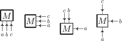
Figure 1: Graphical representations of $M_{abc}$, which are supposed to be equivalent. Here vacant edges are drawn in thick bold lines to clarify the definition. Reading off the indices on a particular box is always done in a counter-clockwise manner.

In general, the correspondence between a multi-index variable and a graph is defined by the following rules:

• A variable is represented by a box containing its label.

• Indices of a variable are assigned counter-clockwise on arrows attached to a box.

• The first index of a variable is assigned to the arrow which appears first after vacant edges of a box in the counter clockwise direction. Here, vacant edges mean those with no arrows attached, and must form a connected bunch for well-definedness (see Figure 1).

It is convenient to associate a sign to a crossing of two lines as in Figure 2. A merit of this convention is to simplify the symmetric condition (2.4): signs coming from reordering of indices of a symmetric tensor can be represented by crossings as in Figure 3. The convention also simplifies the anti-symmetric condition (2.5) as in Figure 4. We also have a graphical identity Figure 5 corresponding to the last equation of (3.2).

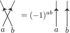
Figure 2: The sign associated to a crossing.

Figure 3: The symmetric condition (2.4) in terms of graphs. This holds for $P$ as well.

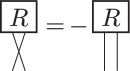
Figure 4: The anti-symmetric condition (2.5) in terms of graphs.

Figure 5: The identity to reverse an orientation of an arrow corresponding to the last equation of (3.2). The sign is represented by the self-crossing due to $(-1)^{aa}=(-1)^{a}$.

A very convenient graphical identity which will be used frequently in later computations is shown in Figure 6. This identity allows one to change order of variables. The identity for the simplest case of the first equality can be proven by

$$A^{ab}B_{b}{}^{c} =(-1)^{(a+b)(b+c)}B_{b}{}^{c}A^{ab}$$

$$=(-1)^{(a+b)(b+c)+b}B^{bc}A^{a}{}_{b}$$

$$=(-1)^{ab+bc+ca}B^{bc}A^{a}{}_{b},$$ (3.3)

where we have used $|A^{ab}|=|a|+|b|,\ |B_{b}{}^{c}|=|b|+|c|\ \hbox{mod 2}$ for (2.2) and (3.2) for the index $b$. Here, the nice thing is that the cumbersome sign in the last line of (3.3) are accounted graphically by the crossings of the arrows. The proof can obviously be generalized to other cases. In fact, the identity shown in the Figure 6 is a representative of various variants of the identity: some of $A,B,C$ or the double-line arrows may be absent, double-line arrows may contain anti-parallel arrows, and there may exist other crossings of arrows. As illustrations, two of such variants are shown in Figure 7. Basically, all the computations in the following sections can be performed by mostly using the variants of the identity and the basic properties of variables.

Figure 6: An identity for reordering variables. In the above figure, $A,B,C$, and the double-line arrows represent bunches of variables and arrows, respectively. The identity still holds, even when some of $A,B,C$ or the double-line arrows are absent, when bunches of arrows contain anti-parallel arrows, and when arrows cross in other ways. The essential points are (i) Before and after reordering, connections and directions of arrows must be kept, except for those connecting reordered variables. (ii) As for the arrows connecting reordered variables, they must be reconnected with reversed directions in the ways shown in the figure.

Finally, we will show the graphical representation of the fundamental Poisson bracket. By using the Leibniz rule (2.16), the computation of a Poisson bracket between arbitrary quantities can be reduced to summation of terms containing only the fundamental Poisson bracket. The graphical representation of the fundamental Poisson bracket is given in Figure 8. As in the figure, we use a dashed line to indicate a pair of $M,P$ between which the fundamental Poisson bracket is taken. An advantage of this graphical representation is that the cumbersome signs appearing in (2.9) can be represented by the crossings due to the sign assignment Figure 2.

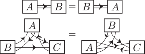
Figure 7: Two examples of variants of the identity shown in Figure 6.

Figure 8: The graphical representation of the fundamental Poisson bracket (2.9). It is given by the summation of the six graphs in the figure. The dashed line indicates the pair between which the fundamental Poisson bracket is taken. The cumbersome signs in (2.9) are represented by the sign assignment Figure 2 to the crossings.

4 The Poisson algebra of the constraints

In this section, we define the constraints in the super-extended case, and show the Poisson algebra satisfied by them. It turns out that the constraints as well as the constraint Poisson algebra are formally unchanged from the purely bosonic case, in the sense that the overall structure of the constraints and the algebra satisfied by them is very much similar (modulo signs). This formal simplicity would be due to the validity and consistency of the basic properties imposed on the parameters and dynamical variables in the previous sections.

By simply transferring the purely bosonic case to the present super-extended case by taking care of index orderings, we consider the Hamiltonian constraints defined by

$${{\cal H}}_{a}=\frac{1}{2}\left(P_{a}{}^{bc}P_{c}{}^{de}M_{edb}-\lambda M_{a}{}^{b}{}_{b}\right),$$ (4.1)

where $\lambda$ is a real constant. It was shown in the purely bosonic case that $\lambda$ can be interpreted as a cosmological constant, because the $N=1$ case in CTM exactly reproduces the mini-superspace approximation of general relativity with a cosmological constant proportional to $\lambda$ [42]. For this reason, we call $\lambda$ in this case also to be the cosmological constant.

It is convenient at this point to introduce a non-dynamical variable $T^{a}$, and consider

$$H(T)=T^{a}{{\cal H}}_{a}=\frac{1}{2}\left(T^{a}P_{a}{}^{bc}P_{c}{}^{de}M_{edb}-\lambda T^{a}M_{a}{}^{b}{}_{b}\right).$$ (4.2)

For convenience, we separately consider the two terms by defining $H_{0}(T)=\left.H(T)\right|_{\lambda=0}$. Similarly, the momentum constraints are given by

$$J(R)=-\frac{1}{2}R^{ab}P_{b}{}^{cd}M_{dca},$$ (4.3)

where $R$ is a non-dynamical matrix variable with the anti-symmetric property (2.5), and the overall minus sign is for convenience. The graphical representations of the constraints are depicted diagrammatically in Figure 9 up to the numerical factors.

Figure 9: The graphical representations of $H(T)$ in (4.2) and $J(R)$ in (4.3) are given by the left and the right figures, respectively, up to the numerical factors.

The constraint algebra is worked out explicitly by using the diagrammatic notation in Appendix A. The result is that the constraints form a set of first-class constraints, satisfying the following first-class Poisson algebra,

$$\{H(T_{1}),H(T_{2})\}=J([\tilde{T}_{1},\tilde{T}_{2}]+2\lambda\,T_{1}\wedge T_{2}),$$ (4.4)

$$\{H(T),J(R)\}=H(TR),$$ (4.5)

$$\{J(R_{1}),J(R_{2})\}=J([R_{1},R_{2}]),$$ (4.6)

where the matrix commutator is defined in (2.8), $\tilde{T}_{ab}=T^{c}P_{cab}$, $(T_{1}\wedge T_{2})^{ab}=T_{1}^{a}T_{2}^{b}-T_{2}^{a}T_{1}^{b}$, and $(TR)_{a}=T^{b}R_{ba}$.

The consistency that the arguments of $J$ be anti-symmetric on the right-hand side of (4.4) and (4.6) can be checked from

$$(\tilde{T}_{1}\tilde{T}_{2})^{ab}=T_{1}^{c}P_{c}{}^{ad}T_{2}^{e}P_{ed}{}^{b}=(-1)^{(d+b)(a+d)+bd+ad+d}T_{2}^{e}P_{e}{}^{bd}T_{1}^{c}P_{cd}{}^{a}=(-1)^{ab}(\tilde{T}_{2}\tilde{T}_{1})^{ba},$$ (4.7)

$$(R_{1}R_{2})^{ab}=R_{1}^{ac}R_{2}{}_{c}{}^{b}=(-1)^{(a+c)(b+c)+ac+bc+c}R_{2}^{bc}R_{1}{}_{c}{}^{a}=(-1)^{ab}(R_{2}R_{1})^{ba}.$$ (4.8)

In the case of $\lambda=0$, one can add another constraint given by

$$D=\frac{1}{6}P^{abc}M_{cba}.$$ (4.9)

This satisfies $\{D,P_{abc}\}=P_{abc},\ \{D,M_{abc}\}=-M_{abc}$, and $D$ is therefore a dilatational constraint. Such a dilatational constraint played a vital role in the connection between CTM and statistical systems on random networks, i.e. randomly connected tensor networks [44, 45, 46]. From the dilatational property of $D$, it is obvious that $D$ forms a first-class constraint algebra with $H_{0}$ and $J$ as

$$\{D,H_{0}(T)\}=H_{0}(T),$$ (4.10)

$$\{D,J(R)\}=0.$$ (4.11)

5 Reality condition

The minimal set of dynamical variables of the purely bosonic CTM consist of a canonical conjugate pair of rank-three real symmetric tensors $M,P$. To consider this minimal setting also in the super-extended case, we will impose reality conditions on the super-extended variables in this section. We will also check the consistency of the reality conditions with the constraints.

We denote the complex conjugation of a variable $A$ by $A^{*}$, and impose that

$$(A_{1}A_{2}\ldots A_{n})^{*}=A_{n}^{*}A_{n-1}^{*}\ldots A_{1}^{*}$$ (5.1)

for the complex conjugate of a product of variables $A_{i}$. We consider $\Omega$ to be real for even index values, and pure imaginary for odd ones, respectively (note that, from the definition (2.6), $\Omega$ does not have Grassmann odd components.). From this demand, we obtain the complex conjugate of the $\Omega$:

$$\Omega_{ab}^{*}=(-1)^{ab}\Omega_{ab}=\Omega_{ba},$$

$$\Omega^{ab}{}^{*}=(-1)^{ab}\Omega^{ab}=\Omega^{ba},$$ (5.2)

where (2.6) should also be reminded. It is important to notice that the complex conjugation is generally not commutative with raising and lowering indices. This can be seen by

$$(A_{a})^{*}=(A^{b}\Omega_{ba})^{*}=\Omega_{ab}A^{b*}\neq A^{b*}\Omega_{ba}\hbox{ in general}.$$ (5.3)

Therefore, the definition of the complex conjugation of $A$ depends on whether it is defined by upper or lower components. We also obtain

$$(A^{a}B_{a})^{*}=(A_{a}\Omega^{ab}B_{b})^{*}=B_{b}^{*}\Omega^{ba}A_{a}^{*}=B^{*a}A^{*}_{a}.$$ (5.4)

Graphically, this is

$$(A\rightarrow-B)^{*}=B^{*}\rightarrow-A^{*},$$ (5.5)

namely, the complex conjugation is a reflection in the horizontal direction, but with reversed connections of arrows. Here, as mentioned above, it is important to define the complex conjugations of variables for fixed positions (upper or lower) of their indices. Thus, throughout this paper, we define the complex conjugation of tensors (vectors and matrices as well) by its lower components. For example, $A^{*}{}_{a}=A_{a}^{*}$, and $A^{*a}=A_{b}^{*}\Omega^{ba}$, as used in (5.4). One could define the complex conjugation of a variable by its upper components as well, but mixtures of the two ways of definitions would lead to unnecessary complications.

From the reflection property (5.5) of the complex conjugation, it is natural to define the reality/imaginary condition in the case of tensors to be the one dictating its relation with the tensor with reversed indices:

$$T_{a_{1}a_{2}\ldots a_{p}}^{*}=\pm T_{a_{p}a_{p-1}\ldots a_{1}}.$$ (5.6)

This is indeed what was imposed on $\Omega$ in (5.2) with a plus sign. We impose the reality conditions on the dynamical variables as

$$M_{abc}^{*}=M_{cba},$$

$$P_{abc}^{*}=P_{cba}.$$ (5.7)

The reality conditions on the non-dynamical variables are given by

$$T_{a}^{*}=T_{a},$$

$$R_{ab}^{*}=-R_{ba}=(-1)^{ab}R_{ab},$$ (5.8)

where (2.5) should also be reminded. Because of the anti-symmetry (2.5) of $R$, we have to consider the reality condition with a minus sign in (5.8) to recover the usual reality condition in the purely bosonic case.

Figure 10: The proof of reality of $J(R)$.

The proof of the reality of the constraints is straightforward. The proof for $J(R)$ is shown in Figure 10. The first graph is obtained from the one of $J(R)$ in Figure 9 by taking its reflection with reversed arrows, and its minus sign comes from (5.8). The second one is obtained by using variants of the reordering identity Figure 6. Finally, the third one is obtained by the symmetric/anti-symmetric properties of the variables, Figure 3 and 4. The proof for the reality of $H_{0}(T)$ proceeds basically along the same lines, as shown in Figure 11.

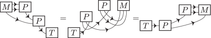
Figure 11: The proof of reality of $H_{0}(T)$.

It is also easy to show the reality of the cosmological constant term in (4.2), and the dilatational constraint (4.9).

Finally, we should check whether the reality conditions are satisfied for the arguments of the constraints on the right-hand sides of the constraint algebra (4.4), (4.5), and (4.6):

$$(\tilde{T}_{1}\tilde{T}_{2})_{ab}^{*}=(T_{1}^{c}P_{ca}{}^{d}T_{2}^{e}P_{edb})^{*}=P_{b}{}^{de}T_{2e}P_{da}{}^{c}T_{1c}=(-1)^{ab}T_{1}^{c}P_{ca}{}^{d}T_{2}^{e}P_{edb}=(-1)^{ab}(\tilde{T}_{1}\tilde{T}_{2})_{ab},$$

$$(T_{1a}T_{2b})^{*}=T_{2b}T_{1a}=(-1)^{ab}T_{1a}T_{2b},$$

$$(TR)^{*}_{a}=(T^{b}R_{ba})^{*}=-R_{a}{}^{b}T_{b}=T^{b}R_{ba},$$

$$(R_{1}R_{2})_{ab}^{*}=(R_{1a}{}^{c}R_{2cb})^{*}=R_{2b}{}^{c}R_{1ca}=(-1)^{ab}R_{1a}{}^{c}R_{2cb}=(R_{1}R_{2})_{ab},$$ (5.9)

where we have used (5.7), (5.8), and (5.4) concerning the complex conjugation, and have reordered the variables and indices with attention to the signs using (2.2), (2.4), (2.5), and (3.2).

6 Quantization

In this section, we carry out the quantization of the classical system discussed so far. The quantized operator corresponding to a classical quantity $A$ will be denoted by $\hat{A}$, and the same $Z_{2}$ grade will be assigned, i.e. $|\hat{A}|=|A|$. We assume the same symmetric properties (2.4) for the quantized dynamical variables $\hat{M},\hat{P}$. As for the reality condition, we impose

$$\hat{M}_{abc}^{\dagger}=\hat{M}_{cba},$$

$$\hat{P}_{abc}^{\dagger}=\hat{P}_{cba},$$ (6.1)

similar to (5.7), where $\hat{A}^{\dagger}$ denotes the Hermitian conjugate of $\hat{A}$. A reflection property similar to (5.4) holds, since

$$(\hat{f}^{a}\hat{g}_{a})^{\dagger}=(\hat{f}_{a}\Omega^{ab}\hat{g}_{b})^{\dagger}=\hat{g}_{b}^{\dagger}(\Omega^{ab})^{*}\hat{f}_{a}^{\dagger}=\hat{g}_{b}^{\dagger}\Omega^{ba}\hat{f}_{a}^{\dagger}=\hat{g}^{\dagger a}\hat{f}^{\dagger}_{a},$$ (6.2)

where we should note that $(\hat{g}^{a}){}^{\dagger}\neq\hat{g}^{\dagger a}$ in general, if $\hat{g}^{\dagger}$ is defined through its lower components. The definition of the Hermitian conjugate with lower components is assumed throughout this paper, as the complex conjugation in Section 5.

The fundamental commutator is defined by

$$[\hat{M}_{abc},\hat{P}^{def}]=-[\hat{P}_{abc},\hat{M}^{def}]=i\,\delta_{abc}^{fed},$$ (6.3)

$$[\hat{M}_{abc},\hat{M}^{def}]=[\hat{P}_{abc},\hat{P}^{def}]=0,$$ (6.4)

where $[\ ,\ ]$ is the operator commutator,

$$[\hat{A},\hat{B}]=\hat{A}\hat{B}-(-1)^{|A||B|}\hat{B}\hat{A}.$$ (6.5)

The commutator satisfies

$$[\hat{A},\hat{B}]=-(-1)^{|A||B|}[\hat{B},\hat{A}].$$ (6.6)

By assuming the associativity of products of operators, one can readily prove the Leibniz rule,

$${}[\hat{A}\hat{B},\hat{C}]=\hat{A}[\hat{B},\hat{C}]+(-1)^{|B||C|}[\hat{A},\hat{C}]\hat{B},$$

$${}[\hat{A},\hat{B}\hat{C}]=[\hat{A},\hat{B}]\hat{C}+(-1)^{|A||B|}\hat{B}[\hat{A},\hat{C}],$$ (6.7)

and the Jacobi identity in the operator language,

$${}[[\hat{A},\hat{B}],\hat{C}]=[\hat{A},[\hat{B},\hat{C}]]+(-1)^{|B||C|}[[\hat{A},\hat{C}],\hat{B}].$$ (6.8)

Note that the Leibniz rules (6.7) have the same form as the classical ones (2.16). This means that the computation of the commutation algebra of the quantized constraints proceeds exactly in the same manner as the classical case, if the orders of $\hat{M},\hat{P}$ are not changed during the computation, since the classical Poisson algebra (4.4), (4.5), (4.6), (4.10), and (4.11) of the constraints can in principle be derived solely by using (2.9) and (2.16). As will be discussed in due course, this fact will ensure that the classical Poisson algebra can be translated without any essential modifications to a quantum commutation algebra.

As the reality condition on the classical constraints, we impose Hermiticity on the quantized constraints. By replacing the variables in (4.2), (4.3) with the quantized ones and taking into account the possible normal ordering term, the Hermiticity condition determines the quantized Hamiltonian and momentum constraints as

$$\hat{H}(T)=\frac{1}{2}T^{a}\left(\hat{P}_{a}{}^{bc}\hat{P}_{c}{}^{de}\hat{M}_{edb}+i\lambda_{H}\hat{P}_{a}{}^{b}{}_{b}-\lambda\hat{M}_{a}{}^{b}{}_{b}\right),$$ (6.9)

$$\hat{J}(R)=-\frac{1}{2}R^{ab}\hat{P}_{b}{}^{cd}\hat{M}_{dca},$$ (6.10)

$$\hat{D}=\frac{1}{6}\left(\hat{P}^{abc}\hat{M}_{cba}+i\lambda_{D}\right),$$ (6.11)

where $\lambda_{H},\ \lambda_{D}$ are real constants coming from the normal ordering, and will be determined below. As will be checked below, there are no normal ordering terms for $\hat{J}(R)$.

Let us first check the Hermiticity of $\hat{J}(R)$. By taking the Hermitian conjugate, we obtain

$$\hat{J}(R)^{\dagger} =-\frac{1}{2}\hat{M}^{acd}\hat{P}_{dc}{}^{b}R_{ba}$$

$$=\hat{J}(R)-\frac{1}{2}[\hat{M}^{acd},\hat{P}_{dc}{}^{b}]R_{ba}.$$ (6.12)

where we have used (5.8), (6.1), and (6.2). From (6.3), it is obvious that the second term can only produce either $R_{ab}\Omega^{ba}$ or $(-1)^{a}R_{ab}\Omega^{ba}=R_{ab}\Omega^{ab}$, which both vanish due to the symmetry/anti-symmetry properties of $R,\Omega$. Therefore, (6.10) is Hermite.

To study the Hermiticity of the quantized Hamiltonian constraint, let us take the Hermitian conjugate of the first term of (6.9). Similarly as above, we obtain

$$\left(T^{a}\hat{P}_{a}{}^{bc}\hat{P}_{c}{}^{de}\hat{M}_{edb}\right)^{\dagger}=\hat{M}^{bde}\hat{P}_{ed}{}^{c}\hat{P}_{cb}{}^{a}T_{a}=T^{a}\hat{P}_{a}{}^{bc}\hat{P}_{c}{}^{de}\hat{M}_{edb}+(\hbox{Figure~{}\ref{fig:orderH}}),$$ (6.13)

where the normal ordering terms are shown in Figure 12.

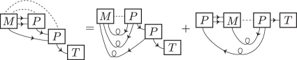
Figure 12: Computation of the normal ordering term in $\hat{H}(T)$. The dashed lines indicate the pairs of $\hat{M},\hat{P}$, between which the fundamental commutators are taken.

Here, we have used some variants of the identity stated in Figure 6, and have also reversed the orientations of some of the arrows by using the rule given in Figure 5. By making use of Figure 8, we obtain a sum of graphs which contain the elementary ones shown in Figure 13. The left graph produces a numerical factor $\sum_{a}(-1)^{a}=N-\tilde{N}$, while the right $(-1)^{2a}\delta_{a}^{b}=\delta_{a}^{b}$. By summing over all the contributions, we obtain

$$(\hbox{Figure}~{}\ref{fig:orderH})=(N-\tilde{N}+2)(N-\tilde{N}+3)\,T^{a}P_{a}{}^{b}{}_{b}.$$ (6.14)

Therefore, the Hermiticity of $\hat{H}(T)$ is obtained by putting

$$\lambda_{H}=\frac{1}{2}(N-\tilde{N}+2)(N-\tilde{N}+3).$$ (6.15)

One can see in this expression that the fermionic degrees of freedom contribute in an opposite manner to the bosonic ones, as commonly argued.

Figure 13: By substituting the fundamental commutator into Figure 12, one obtains some graphs containing the elementary ones shown in the figure.

In the same manner, we obtain

$$\lambda_{D}=\frac{1}{2}(N-\tilde{N})(N-\tilde{N}+1)(N-\tilde{N}+2).$$ (6.16)

As discussed above, the computation of the commutation algebra of the quantized constraints is basically the same as the classical one, if we keep the ordering of $\hat{M},\hat{P}$, because of the formal equivalence between the identities satisfied by the Poisson bracket and the commutator. We take the normal ordering that $\hat{M}$ be always on the rightmost if it exists, as the expressions of $\hat{H}(T),\hat{J}(R),\hat{D}$ in (6.9), (6.10), (6.11). Under this convention of ordering, the same part of the quantized constraints as the classical ones generate the same algebra as the classical case. The only difference between the quantum and classical constraints is the existence of the normal ordering term proportional to $\hat{P}_{a}{}^{b}{}_{b}$ in $\hat{H}$ in (6.9). As we will see below, this extra term does not change the commutation algebra. In Figure 14, we show the graphs which are produced from the commutator with $\hat{H}_{0}$, namely $[T_{1}^{a}\hat{P}_{a}{}^{bc}\hat{P}_{c}{}^{de}\hat{M}_{edb},T_{2}^{a}\hat{P}_{a}{}^{b}{}_{b}]$. All the terms in Figure 14 are symmetric under $T_{1}\leftrightarrow T_{2}$, and therefore cancel out in the computation of $[\hat{H}(T_{1}),\hat{H}(T_{2})]$.

Figure 14: The terms generated from the commutator $[T_{1}^{a}\hat{P}_{a}{}^{bc}\hat{P}_{c}{}^{de}\hat{M}_{edb},T_{2}^{a}\hat{P}_{a}{}^{b}{}_{b}]$.

Moreover, the normal ordering term does not either cause problems with the cosmological constant term, since the commutator between them can only produce the kinds of terms, $T_{1}^{a}T_{2a}$ or $T_{1}^{a}T_{2a}(-1)^{a}$, which are symmetric under $T_{1}\leftrightarrow T_{2}$. One can also check the covariant property of the normal ordering term with $\hat{J}(R)$, and the commutator with $\hat{D}$. Thus, we finally obtain the following quantum constraint commutation algebra, basically the same as the classical one,

$$[\hat{H}(T_{1}),\hat{H}(T_{2})]=\hat{J}([\hat{T}_{1},\hat{T}_{2}]+2\lambda\,T_{1}\wedge T_{2}),$$ (6.17)

$$[\hat{H}(T),\hat{J}(R)]=\hat{H}(TR),$$ (6.18)

$$[\hat{J}(R_{1}),\hat{J}(R_{2})]=\hat{J}([R_{1},R_{2}]),$$ (6.19)

$$[\hat{D},\hat{H}_{0}(T)]=\hat{H}_{0}(T),$$ (6.20)

$$[\hat{D},\hat{J}(R)]=0,$$ (6.21)

where $\hat{T}_{ab}=T^{c}\hat{P}_{cab}$, and $\hat{H}_{0}(T)=\hat{H}(T)|_{\lambda=0}$. Here, note that the argument of $\hat{J}$ on the right-hand side of (6.17) contains $\hat{P}$, and therefore is not commutative with the operator part of $\hat{J}$. Hence, we have to carefully put the argument on the leftmost as $R$ in the definition (6.10). As in the bosonic case, the commutation algebra is indeed first-class, and therefore the quantization is consistent.

7 Summary and discussions

In this paper, we have made an attempt to include fermionic degrees of freedom in CTM, which initially was purely bosonic in nature. We have introduced such degrees of freedom by allowing the dynamical rank-three tensors to be either Grassmann even or odd in accordance with the Grassmann natures associated to the indices. This provides a straightforward super-extension of CTM, whose constraints and constraint algebra have basically the same form as the purely bosonic case except for the signs associated to the order of the indices and variables, extending the kinematical symmetry from $O(N)$ to $OSp(N,\tilde{N})$. To prove that the super-extended constraints form a first-class constraint algebra, we have performed an explicit computations of the super-Poisson brackets. This process was facilitated by the graphical expressions which can represent the signs associated to the ordering in a simplified manner. Then, we finally considered the quantization of the super-extended system. It has been shown that, as in the purely bosonic case, the quantized constraint algebra is formally the same as the classical one, which also means that the quantization is consistent. The quantized Hamiltonian constraint contains the normal ordering term proportional to $N-\tilde{N}$, which shows that the bosonic and fermionic degrees of freedom contribute oppositely.

The formalism presented in this paper obviously contains the issue of negative norm states in the quantized case. This issue comes from the Grassmann odd variables. From (6.3) and some basic definitions, one can see that the Grassmann odd variables can be recast into the pairs $\psi^{i},\tilde{\psi}^{i}$ which are hermite, $\psi^{i}=\psi^{i\,\dagger},\tilde{\psi}^{i}=\tilde{\psi}^{i\,\dagger}$, and satisfy the anti-commutation relations, $[\psi^{i},\tilde{\psi}^{j}]_{+}=\delta^{ij},\ [\psi^{i},\psi^{j}]_{+}=[\tilde{\psi}^{i},\tilde{\psi}^{j}]_{+}=0$. Then, one can consider recombinations, $\psi^{i}_{\pm}=\psi^{i}\pm\tilde{\psi}^{i}$, and obtain $[\psi^{i}_{-},\psi^{j}_{-}]_{+}=-2\delta^{ij}$. Since $\psi^{i}_{-}$ is hermite and satisfies the last anti-commutation relation, there exist negative norm states in the Hilbert space.

In order to resolve the issue in the quantized case, some directions of pursuit can be considered. One would be to add constraints like $\psi^{i}-\tilde{\psi}^{i}=0$ which incorporate the fact that the fermionic degrees of freedom should be treated in a first-order Lagrangian. This would require a careful analysis of the full consistency with the original constraints. Another more physically attractive direction would be to pursue the possibility to obtain fermionic degrees of freedom from quantization of bosonic degrees of freedom without initially introducing Grassmann odd variables (see for instance [51] for a recent discussion in such directions). It would be fascinating, if the degrees of freedom of the purely bosonic CTM turn out to generate fermionic ones after quantization. Since fermionic degrees of freedom would be expected to appear as fluctuations around bosonic backgrounds, this would require some analysis of the behavior of the physical wave functions [48] in the vicinity of their peaks. Due to the spin-statistics theorem, it would even be possible that the above two different routes for resolution would finally lead to the same result.

Leaving aside the issue in the quantized case, we would like to stress that the super-extended model presented in this paper itself would have some theoretical interests of its own. One is that, because of its formal equivalence to the purely bosonic case, it would be straightforward to extend the results obtained so far for the purely bosonic case. This would include the exact physical wave functions [47, 48] and the connection with the dual statistical systems, i.e. the randomly connected tensor networks [44, 45, 46]. Especially, since the connection of the latter is based on the classical aspects of CTM, the physical interpretations of the extension would be more solid. Although the additional degrees of freedom would not be real fermions, the super-extensions would provide general hints about how the anti-commuting degrees of freedom would change the physical outcomes compared with the purely bosonic case.

Appendix A Poisson algebra of the constraints

In the following subsections, we will prove the Poisson algebra, (4.4), (4.5), and (4.6) by explicit computations using the graphs introduced in Section 3.

A.1 Computation of $\{J,J\}$

In this subsection, we will compute $\{J(R_{1}),J(R_{2})\}$. The computation of the Poisson bracket between $R_{i}^{ab}P_{b}{}^{cd}M_{dca}\ (i=1,2)$ is shown in Figure 15.

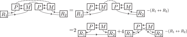
Figure 15: The graphical computation of $\{J(R_{1}),J(R_{2})\}$.

In the first graph, we have moved $R_{2}$ on the rightmost by using a variant of the identity Figure 6 with two variables, and have indicated by the dashed lines the two cases of the fundamental Poisson bracket being taken. As shown in the second graph, one can easily find that the two cases contribute in opposite signs with $R_{1}\leftrightarrow R_{2}$. By substituting the fundamental Poisson bracket Figure 8 into it and considering the symmetry Figure 3 of $P,M$, we obtain the last line. In fact, the second graph of the last line is symmetric under $R_{1}\leftrightarrow R_{2}$ and cancels out.

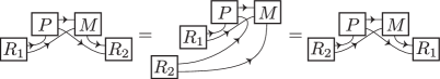
Figure 16: By using a variant of the identity Figure 6, the second graph in the last line of Figure 15 can be shown to be symmetric under $R_{1}\leftrightarrow R_{2}$.

The proof of the symmetric property of the second graph is shown in Figure 16. We therefore finally obtain the result in Figure 17, where the first graph is obtained from the first one in the last line of Figure 15 by moving $R_{2}$ on the leftmost with the use of a variant of the identity Figure 6. By taking care of the sign and the normalization in (4.3), we obtain (4.6).

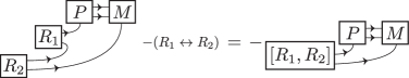
Figure 17: The final result of the computation of Figure 15. The first graph can be obtained from the first one in the last line of Figure 15 by using a variant of the identity Figure 6.

A.2 Computation of $\{H_{0},H_{0}\}$

In this subsection, we consider the $\lambda=0$ case first, and will deal with the $\lambda\neq 0$ case in Appendix A.4.

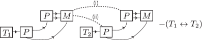
Figure 18: The computation of $\{H_{0},H_{0}\}$. There are two cases, (i) and (ii), of the fundamental Poisson brackets to be taken.

As shown in Figure 18, the Poisson bracket between $T_{i}^{a}P_{a}{}^{bc}P_{c}{}^{de}M_{edb}\ (i=1,2)$ is given by the summation of the contributions (i) and (ii) minus the same ones with $T_{1}\leftrightarrow T_{2}$. By comparing with Figure 15, the computation of (i) minus $T_{1}\leftrightarrow T_{2}$ of (i) is basically the same as the computation of $\{J,J\}$ with the replacement $(R_{i}){}_{ab}\rightarrow(\tilde{T}_{i}){}_{ab}=T_{i}^{c}P_{cab}$. Therefore, after taking care of the sign and the normalization, we obtain the right-hand side of (4.4) with $\lambda=0$. Thus, what remains to show is that the contribution (ii) cancels out with $T_{1}\leftrightarrow T_{2}$ of (ii).

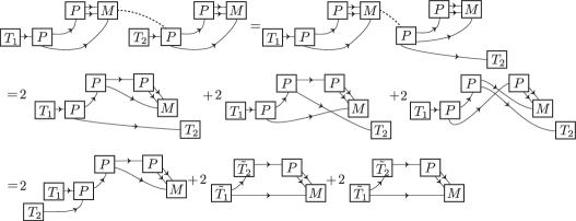
Figure 19: The computation of the contribution (ii) in Figure 18.

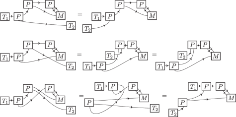
Figure 20: From the second to the third line of Figure 19, each diagram is deformed by using variants of Figure 6 and the symmetry Figure 3 of $M,P$.

In Figure 19, the computation of the contribution (ii) is shown. In the first line, $T_{2}$ is moved on the rightmost by using a variant of the identity Figure 6, and then the fundamental Poisson bracket Fig. 8 is substituted to obtain the second line. From the second to the last line, we use some variants of Figure 6 and Figure 3 to deform each diagram as shown in Figure 20. As shown in Figure 21, the first graph is invariant by itself under $T_{1}\leftrightarrow T_{2}$, and the sum of the last two graphs in Figure 20 is obviously so, too. Therefore, the contribution (ii) cancels out with that of $T_{1}\leftrightarrow T_{2}$.

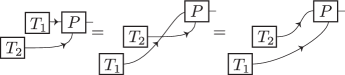
Figure 21: The first graph of the last line in Figure 19 is shown to be invariant under $T_{1}\leftrightarrow T_{2}$ by using a variant of Figure 6 and Figure 3.

A.3 Computation of $\{H_{0},J\}$

In the computation of $\{H_{0}(T),J(R)\}$, there exist three cases of the fundamental Poisson bracket to be taken, as shown in Figure 22.

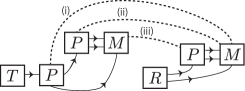
Figure 22: For $\{H_{0}(T),J(R)\}$, there exist three cases of the fundamental Poisson bracket being taken.

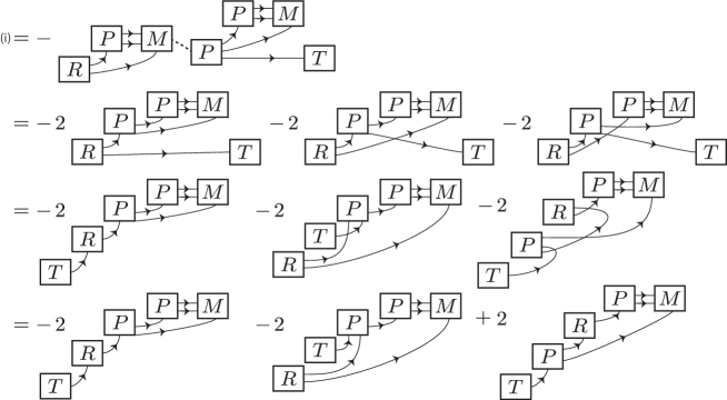
Figure 23: The computation of the contribution (i) in Figure 22. In the first line, we perform an exchange of order, $\{J(R),H_{0}(T)\}=-\{H_{0}(T),J(R)\}$, and move $T$ on the rightmost by using a variant of Figure 6. In the second line, the substitution of the fundamental Poisson bracket Figure 8 results in a sum of three terms due to the symmetric property of $P$. In the third line, some variants of Figure 6 are used to move $T$ in the first and second terms and $T,P$ in the last term. Finally, by using the symmetric and anti-symmetric properties of $P$ and $R$, respectively, we obtain the last line.

The contributions (ii) and (iii) are the same as those appear in the computation of $\{J,J\}$ in Figure 15, if we perform the replacement $R_{1}\rightarrow\tilde{T},\ R_{2}\rightarrow R$. Thus the sum of (ii) and (iii) results in Figure 17 with the replacement. On the other hand, the computation of the contribution (i) is shown in Figure 23. By substituting the fundamental Poisson bracket and using some variants of the identity Figure 6, we obtain the expression of the last line of Figure 23. Here the last two terms cancel with the contributions (ii) and (iii), namely, Figure 17 with $R_{1}\rightarrow\tilde{T},\ R_{2}\rightarrow R$. Therefore, only the first term remains for $\{H_{0}(T),J(R)\}$. By taking care of the normalization and the sign of (4.3), one obtains (4.5).

A.4 Cosmological constant term

Here we consider the cosmological constant term. The difference between $\{H,H\}$ and $\{H_{0},H_{0}\}$ is

$$\{H(T_{1}),H(T_{2})\}-\{H_{0}(T_{1}),H_{0}(T_{2})\}=-\frac{\lambda}{2}\,\{H_{0}(T_{1}),T_{2}^{a}M_{a}{}^{bc}\Omega_{cb}\}-(T_{1}\leftrightarrow T_{2}).$$ (A.1)

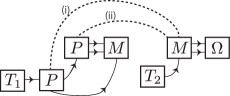
Figure 24: The computation of $\{H_{0}(T_{1}),T_{2}^{a}M_{a}{}^{bc}\Omega_{cb}\}$. There are two contributions of the fundamental Poisson bracket.

The computation of the first term on the right-hand side can be represented by Figure 24. There are two contributions (i) and (ii) of the fundamental Poisson bracket.

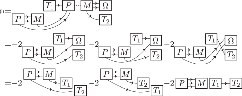
Figure 25: The computation of (i) in Figure 24. The result is symmetric under $T_{1}\leftrightarrow T_{2}$, and cancels out.

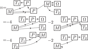
Figure 26: The computation of (ii) in Figure 24. The second term in the last line is symmetric under $T_{1}\leftrightarrow T_{2}$, and cancels out. On the other hand, the first term generates the momentum constraint with the $T_{1}\leftrightarrow T_{2}$ term.

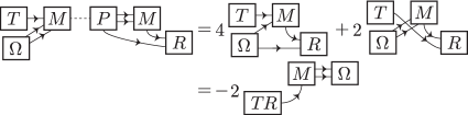
Figure 27: The Poisson bracket between the cosmological constant term and $J(R)$. The first graph on the right-hand side of the first line vanishes because of the symmetry/anti-symmetry properties of $M,R$.

As shown by the graphical computation of Figure 25, the contribution (i) turns out to be symmetric under $T_{1}\leftrightarrow T_{2}$, and hence cancels out. Here, note that, since $\Omega$ is bosonic, we do not need to take care of the horizontal locations of $\Omega$ in the graphical expression. The computation of the contribution (ii) is shown in Figure 26. The second term in the last line is symmetric and cancels out. On the other hand, with the $T_{1}\leftrightarrow T_{2}$ term, the first term generates $J(2\lambda\,T_{1}\wedge T_{2})$ after taking into account the normalization and the sign. This is actually the term proportional to $\lambda$ on the right-hand side of (4.4).

We can also check (4.5). The computation of the additional term proportional to $\lambda$ is given in Figure 27.

Acknowledgements

The work of NS was supported in part by JSPS KAKENHI Grant Number 15K05050. GN would like to thank NS for supporting his visit to YITP, where this work was started. GN would like to thank his host Prof. K. S. Narain and Prof. Herman Nicolai for providing support and hospitality during his stay at ICTP and Max-Planck Institute for Gravitational Physics (AEI), Golm, respectively, where a part of the work was done. NS would like to thank Daniele Oriti for the hospitality and support at his stay in the latter institute. We are grateful to Yuki Sato for several useful discussions during the course of this work.

References

- [1] J. Ambjorn, B. Durhuus and T. Jonsson, “Three-Dimensional Simplicial Quantum Gravity And Generalized Matrix Models,” Mod. Phys. Lett. A 6, 1133 (1991).
- [2] N. Sasakura, “Tensor Model For Gravity And Orientability Of Manifold,” Mod. Phys. Lett. A 6, 2613 (1991).
- [3] N. Godfrey and M. Gross, “Simplicial Quantum Gravity In More Than Two-Dimensions,” Phys. Rev. D 43, 1749 (1991).
- [4] M. Fukuma, S. Sugishita and N. Umeda, “Putting matters on the triangle-hinge models,” arXiv:1504.03532 [hep-th].
- [5] M. Fukuma, S. Sugishita and N. Umeda, “Random volumes from matrices,” JHEP 1507, 088 (2015) [arXiv:1503.08812 [hep-th]].
- [6] P. Di Francesco, P. H. Ginsparg and J. Zinn-Justin, “2-D Gravity and random matrices,” Phys. Rept. 254, 1 (1995) [hep-th/9306153].
- [7] D. V. Boulatov, “A Model of three-dimensional lattice gravity,” Mod. Phys. Lett. A 7, 1629 (1992) [arXiv:hep-th/9202074].
- [8] H. Ooguri, “Topological lattice models in four-dimensions,” Mod. Phys. Lett. A 7, 2799 (1992) [arXiv:hep-th/9205090].
- [9] R. De Pietri, L. Freidel, K. Krasnov and C. Rovelli, “Barrett-Crane model from a Boulatov-Ooguri field theory over a homogeneous space,” Nucl. Phys. B 574, 785 (2000) [arXiv:hep-th/9907154].
- [10] L. Freidel, “Group field theory: An Overview,” Int. J. Theor. Phys. 44, 1769 (2005) [hep-th/0505016].
- [11] D. Oriti, “The microscopic dynamics of quantum space as a group field theory,” arXiv:1110.5606 [hep-th].
- [12] R. De Pietri and C. Petronio, “Feynman diagrams of generalized matrix models and the associated manifolds in dimension 4,” J. Math. Phys. 41, 6671 (2000) [gr-qc/0004045].
- [13] R. Gurau, “Colored Group Field Theory,” Commun. Math. Phys. 304, 69 (2011) [arXiv:0907.2582 [hep-th]].
- [14] R. Gurau and J. P. Ryan, “Colored Tensor Models - a review,” SIGMA 8, 020 (2012) [arXiv:1109.4812 [hep-th]].
- [15] D. Benedetti and R. Gurau, “Symmetry breaking in tensor models,” arXiv:1506.08542 [hep-th].
- [16] T. Delepouve and R. Gurau, “Phase Transition in Tensor Models,” JHEP 1506, 178 (2015) [arXiv:1504.05745 [hep-th]].
- [17] V. Bonzom, T. Delepouve and V. Rivasseau, “Enhancing non-melonic triangulations: A tensor model mixing melonic and planar maps,” Nucl. Phys. B 895, 161 (2015) [arXiv:1502.01365 [math-ph]].
- [18] T. Delepouve and V. Rivasseau, “Constructive Tensor Field Theory: The Model,” arXiv:1412.5091 [math-ph].
- [19] V. A. Nguyen, S. Dartois and B. Eynard, “An analysis of the intermediate field theory of T4 tensor model,” JHEP 1501, 013 (2015) [arXiv:1409.5751 [math-ph]].
- [20] D. Benedetti and V. Lahoche, “Functional Renormalization Group Approach for Tensorial Group Field Theory: A Rank-6 Model with Closure Constraint,” arXiv:1508.06384 [hep-th].
- [21] R. C. Avohou, V. Rivasseau and A. Tanasa, “Renormalization and Hopf Algebraic Structure of the 5-Dimensional Quartic Tensor Field Theory,” arXiv:1507.03548 [math-ph].
- [22] J. B. Geloun, “A power counting theorem for a tensorial group field theory,” arXiv:1507.00590 [hep-th].
- [23] V. Lahoche, D. Oriti and V. Rivasseau, “Renormalization of an Abelian Tensor Group Field Theory: Solution at Leading Order,” JHEP 1504, 095 (2015) [arXiv:1501.02086 [hep-th]].
- [24] D. Benedetti, J. Ben Geloun and D. Oriti, “Functional Renormalisation Group Approach for Tensorial Group Field Theory: a Rank-3 Model,” JHEP 1503, 084 (2015) [arXiv:1411.3180 [hep-th]].
- [25] J. Ben Geloun and R. Toriumi, “Parametric Representation of Rank d Tensorial Group Field Theory: Abelian Models with Kinetic Term ,” arXiv:1409.0398 [hep-th].
- [26] V. Bonzom, R. Gurau, A. Riello and V. Rivasseau, “Critical behavior of colored tensor models in the large N limit,” Nucl. Phys. B 853, 174 (2011) [arXiv:1105.3122 [hep-th]].
- [27] R. Gurau and J. P. Ryan, “Melons are branched polymers,” Annales Henri Poincare 15, no. 11, 2085 (2014) [arXiv:1302.4386 [math-ph]].
- [28] M. Raasakka and A. Tanasa, “Next-to-leading order in the large expansion of the multi-orientable random tensor model,” Annales Henri Poincare 16, no. 5, 1267 (2015) [arXiv:1310.3132 [hep-th]].
- [29] S. Dartois, R. Gurau and V. Rivasseau, “Double Scaling in Tensor Models with a Quartic Interaction,” JHEP 1309, 088 (2013) [arXiv:1307.5281 [hep-th]].
- [30] W. Kamiński, D. Oriti and J. P. Ryan, “Towards a double-scaling limit for tensor models: probing sub-dominant orders,” New J. Phys. 16, 063048 (2014) [arXiv:1304.6934 [hep-th]].
- [31] R. Gurau, “The 1/N Expansion of Tensor Models Beyond Perturbation Theory,” Commun. Math. Phys. 330, 973 (2014) [arXiv:1304.2666 [math-ph]].
- [32] J. Ambjorn, J. Jurkiewicz and R. Loll, “Emergence of a 4-D world from causal quantum gravity,” Phys. Rev. Lett. 93 (2004) 131301 [hep-th/0404156].
- [33] N. Sasakura, “Canonical tensor models with local time,” Int. J. Mod. Phys. A 27 (2012) 1250020 [arXiv:1111.2790 [hep-th]].
- [34] N. Sasakura, “Uniqueness of canonical tensor model with local time,” Int. J. Mod. Phys. A 27 (2012) 1250096 [arXiv:1203.0421 [hep-th]].
- [35] N. Sasakura, “A canonical rank-three tensor model with a scaling constraint,” Int. J. Mod. Phys. A 28 (2013) 1 [arXiv:1302.1656 [hep-th]].
- [36] D. Oriti, “Group field theory as the 2nd quantization of Loop Quantum Gravity,” arXiv:1310.7786 [gr-qc].
- [37] R. L. Arnowitt, S. Deser and C. W. Misner, “Canonical variables for general relativity,” Phys. Rev. 117, 1595 (1960).
- [38] R. L. Arnowitt, S. Deser and C. W. Misner, “The Dynamics of general relativity,” arXiv:gr-qc/0405109.
- [39] B. S. DeWitt, “Quantum Theory of Gravity. 1. The Canonical Theory,” Phys. Rev. 160, 1113 (1967).
- [40] S. A. Hojman, K. Kuchar and C. Teitelboim, “Geometrodynamics Regained,” Annals Phys. 96, 88 (1976).
- [41] C. Teitelboim and J. Zanelli, “Dimensionally continued topological gravitation theory in Hamiltonian form,” Class. Quant. Grav. 4, L125 (1987).
- [42] N. Sasakura and Y. Sato, “Interpreting canonical tensor model in minisuperspace,” Phys. Lett. B 732, 32 (2014) [arXiv:1401.2062 [hep-th]].
- [43] N. Sasakura and Y. Sato, “Constraint algebra of general relativity from a formal continuum limit of canonical tensor model,” arXiv:1506.04872 [hep-th].
- [44] N. Sasakura and Y. Sato, “Renormalization procedure for random tensor networks and the canonical tensor model,” PTEP 2015, no. 4, 043B09 (2015) [arXiv:1501.05078 [hep-th]].
- [45] N. Sasakura and Y. Sato, “Ising model on random networks and the canonical tensor model,” PTEP 2014, no. 5, 053B03 (2014) [arXiv:1401.7806 [hep-th]].
- [46] N. Sasakura and Y. Sato, “Exact Free Energies of Statistical Systems on Random Networks,” SIGMA 10, 087 (2014) [arXiv:1402.0740 [hep-th]].
- [47] N. Sasakura, “Quantum canonical tensor model and an exact wave function,” Int. J. Mod. Phys. A 28 (2013) 1350111 [arXiv:1305.6389 [hep-th]].
- [48] G. Narain, N. Sasakura and Y. Sato, “Physical states in the canonical tensor model from the perspective of random tensor networks,” JHEP 1501, 010 (2015) [arXiv:1410.2683 [hep-th]].
- [49] N. Sasakura, “Emergent general relativity on fuzzy spaces from tensor models,” Prog. Theor. Phys. 119, 1029 (2008) [arXiv:0803.1717 [gr-qc]].
- [50] N. Sasakura, “Gauge fixing in the tensor model and emergence of local gauge symmetries,” Prog. Theor. Phys. 122, 309 (2009) [arXiv:0904.0046 [hep-th]].
- [51] T. Rempel and L. Freidel, “Interaction Vertex for Classical Spinning Particles,” arXiv:1507.05826 [hep-th].
- [52] B. S. DeWitt, “Supermanifolds,” Cambridge Monographs on Mathematical Physics, Cambridge University Press (1992) 407 p.
- [53] M. Henneaux and C. Teitelboim, “Quantization of gauge systems,” Princeton, USA: Univ. Pr. (1992) 520 p.