Equilibration of hadrons in HICs via Hagedorn States

Abstract

Hagedorn states (HS) are a tool to model the hadronization process which occurs in the phase transition region between the quark gluon plasma (QGP) and the hadron resonance gas (HRG). These states are believed to appear near the Hagedorn temperature $T_{H}$ which in our understanding equals the critical temperature $T_{c}$. A covariantly formulated bootstrap equation is solved to generate the zoo of these particles characterized baryon number $B$, strangeness $S$ and electric charge $Q$. These hadron-like resonances are characterized by being very massive and by not being limited to quantum numbers of known hadrons. All hadronic properties like masses, spectral functions etc. are taken from the hadronic transport model Ultra Relativistic Quantum Molecular Dynamics (UrQMD). Decay chains of single Hagedorn states provide a well description of experimentally observed multiplicity ratios of strange and multi-strange particles. In addition, the final energy spectra of resulting hadrons show a thermal-like distribution with the characteristic Hagedorn temperature $T_{H}$. Box calculations including these Hagedorn states are performed. Indeed, the time scales leading to equilibration of the system are drastically reduced down to 2…5$\,{\rm fm}/c$.

1 Introduction

Back in the 60’s of the last century and before the advent of quantum chromodynamics (QCD) as the theory of strong interactions, R. Hagedorn [1] proposed the existence of a whole zoo of massive, unobserved hadronic resonance states. The spectrum of these particles, known as Hagedorn spectrum, exhibits the specific feature of being exponential in the infinite mass limit with the slope given by the so called Hagedorn temperature $T_{H}$. This temperature denotes the limiting temperature for hadronic matter since any partition function of a HRG with Hagedorn-like mass spectrum diverges as long as $T>T_{H}$. Above the Hagedorn temperature a new state of matter, namely the QGP, shall be realized. Thus, Hagedorn states provide a tool to understand the phase transition from HRG to QGP and back. The Hagedorn states are created in multi-particle collisions most abundantly near $T_{H}$ which in our understanding equals to the critical temperature $T_{c}$. Hagedorn states are color neutral objects which are allowed to have any quantum numbers as long as they are compatible with its mass. The appearance of Hagedorn states in multi-particle collisions and their role was already discussed in [2, 3, 4, 5, 6]. Their appearance near $T_{c}$ can explain, as shown in [4, 5, 6], the fast chemical equilibration of (multi-) strange baryons $B$ and their anti-particles $\bar{B}$ at Relativistic Heavy Ion Collider (RHIC) energies. The inclusion of Hagedorn states in a hadron resonance gas model provides also a lowering of the speed of sound, $c_{s}$ and of the shear viscosity over entropy density ratio $\eta/s$ at the phase transition and being in good agreement with lattice calculations [7, 8, 9, 10].

The starting point of all calculations provided here is the postulate of the statistical bootstrap model (SBM) stating that fireballs consist of fireballs which in turn consist of fireballs etc. . As shown in [11] (cf. also [12]) the mathematical formulation of this postulate in the formulation of [13, 14] leads to the evolving bootstrap equation for the density of states,

$$\tau_{\vec{C}}(m) =\frac{R^{3}}{3\pi\,m}\sum_{\vec{C}_{1},\vec{C}_{2}}\iint{\rm d}m_{1}{\rm d}m_{2}\,m_{1}\tau_{{\vec{C}}_{1}}(m_{1})\,m_{2}\tau_{{\vec{C}}_{2}}(m_{2})\,$$

$$\quad\times\ p_{\rm cm}(m,m_{1},m_{2})\,\delta(\vec{C}-\vec{C}_{1}-\vec{C}_{2})\ ,$$ (1)

where the conservation of the quantum numbers baryon number, strangeness and electrical charge $\vec{C}=(B,S,Q)$ is guaranteed. A major aspect was to restrict on Hagedorn states, which just consist of two constituents in order to allow for generation processes as $2\to 1$ and decay as $1\to 2$. This is some necessary constraint in order to allow for a microscopical calculation in a transport model simulation based on cross sections. The above set of integral equations of Volterra type is solved numerically by disretizing the mass range and consecutively stepping to higher mass bins. The zeroth order input are the known hadrons according their spectral functions as implemented in the transport model UrQMD [15]. The radius $R$ is the only free parameter of the model. Choosing reasonable values as $R=0.8\,{\rm fm}$ ($1.0\,{\rm fm}$) yield Hagedorn temperatures, i.e. the slopes of the exponentially rising Hagedorn spectra $\tau_{\vec{C}}(m)~{}\sim m^{a}\exp(m/T_{H})$ as $T_{H}=162\,{\rm MeV}$ ($145\,{\rm MeV}$) nearly independent of the quantum numbers, as indicated in fig. 1.

In order to treat the decay and the production of Hagedorn states, the decay width $\Gamma$ and the production cross section $\sigma=\pi R^{2}$ are connected via detailed balance as

$$\Gamma_{\vec{C}}(m) =\frac{\sigma}{2\pi^{2}\,\tau_{\vec{C}}(m)}\sum_{\vec{C}_{1},\vec{C}_{2}}\iint{\rm d}m_{1}{\rm d}m_{2}\,\tau_{{\vec{C}}_{1}}(m_{1})\,\tau_{{\vec{C}}_{2}}(m_{2})\,$$

$$\qquad\times\ p_{\rm cm}^{2}(m,m_{1},m_{2})\,\delta(\vec{C}-\vec{C}_{1}-\vec{C}_{2})\ ,$$ (2)

which represents the second major equation of the model. Corresponding Hagedorn spectra and their decay width are shown in fig. 1.

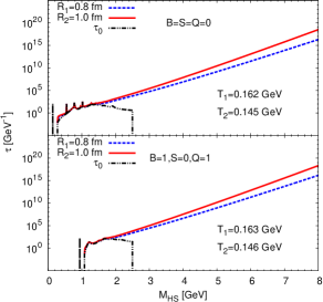
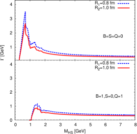
Figure 1: Hagedorn spectrum (left) and total decay width (right) for meson-like $\left(B=S=Q=0\right)$ (upper panel) and baryon-like $\left(B=1,S=0,Q=1\right)$ (lower panel) Hagedorn states.

One observes, that the slope decreases with increasing volume of the Hagedorn state. Correspondingly also the width decreases. Nevertheless, for larger masses, the width is nearly constant in the range of some hundreds of MeV, and also stays finite in the infinite mass limit.

Having the total decay width and the corresponding composition, one is able to calculate the branching ratios for the decay into light Hagedorn states and/or hadrons. Performing such cascading decay simulations, the resulting hadron multiplicity coincide very well with experimentally observed values[11]. This is visualized in fig. 2, where the multiplicity ratios for strange and multi-strange particles are compared with experimental values measured at LHC.

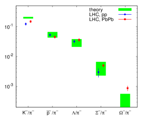
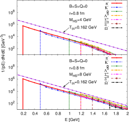
Figure 2: Left: Comparison of particle multiplicity ratios from theory vs. p-p at $\sqrt{s_{NN}}=0.9$$\,{\rm TeV}$ [16] and Pb-Pb at $\sqrt{s_{NN}}=2.76$$\,{\rm TeV}$ [17, 18, 19], both from ALICE at LHC. The bands show the range of calculations from cascade decay of a single charge neutral Hagedorn state with radius $R=0.8\,{\rm fm}$ and initial mass $M_{HS}=4\,{\rm GeV}$ and $M_{HS}=8\,{\rm GeV}$. Right: Energy spectra of hadrons stemming from cascade decay of charge neutral Hagedorn state with radius $R=0.8\,{\rm fm}$ and initial mass $M_{HS}=4\,{\rm GeV}$ and $M_{HS}=8\,{\rm GeV}$.

The most striking result is the fact, that the energy spectra of these decay hadrons look thermal, i.e. the functional behavior is exponential, as shown in fig. 2. The slope parameter coincides with the underlying Hagedorn temperature.

All these ingredients were implemented into UrQMD [15], which can handle the creation and the decay of Hagedorn states and their component dynamically. This enables us to perform box calculations and study the time evolution and the equilibration of the system. The model is able to handle different initialization scenarios, as e.g. the initialization with only nucleons (or pions) with a given particle and energy density. While this may stand for some ’bottom-up’ scenario, alternatively one may start with a given Hagedorn state distribution and look into the resulting hadron distributions. This indicates a ’top-down’ scenario, where the Hagedorn states may stem from some preceding deconfined phase.

Fig. 3 shows the time dependence of kaons and lambdas for box calculations, where only Hagedorn states according to different energy densities were initialized.

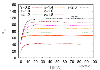
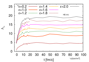
Figure 3: The time dependence of $K^{-}$ (left) and $\Lambda$ hadrons in a box calculation, initialized with Hagedorn states, for different initial energy densities as indicated in the plot.

The given multiplcities at some time are the resulting muliplicities, if all particles would decay down to the stable remnants. One indeed observes very short time scales for the equilibration: While the kaons are almost equilibrated after 2$\,{\rm fm}/c$, the number of lambdas reaches values close to the maximum value already after 5$\,{\rm fm}/c$. Not shown here, but the last statement holds also for nucleons, while pions are even faster equilibrated than the kaons. The multiplicity ratios are almost stable for all energy densities, except for the smallest considered one, i.e. for $\varepsilon=0.2\,{\rm GeV/fm^{3}}$. In addition we find, that the energy spectra of the hadrons again follow an exponential shape, with slope parameters very close to the Hagedorn temperature $T_{H}=162\,{\rm MeV}$, see fig. 4.

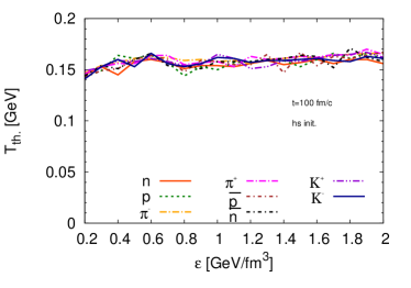
Figure 4: The slope parameter of the energy distribution of different particle species for different initialization energy densities.

We conclude, that Hagedorn states are a valuable tool for the understanding of the phase transition between a deconfined and a hadronic phase. While already the decay particles of one single Hagedorn state look thermal with the Hagedorn temperature as the only scale, a collective system of Hagedorn states leads to small equilibration times of hadrons in the order of few $\,{\rm fm}/c$. These remarkable features may also open the door for alternative descriptions of heavy ion collisions, where directly from a pure gluonic phase without quarks a transition to the confined phase is possible [20].

References

- [1] Hagedorn R 1965 Nuovo Cim. Suppl. 3 147–186
- [2] Greiner C and Leupold S 2001 J. Phys. G 27 L95–L102
- [3] Greiner C, Koch-Steinheimer P, Liu F M, Shovkovy I A and Stoecker H 2005 J. Phys. G 31 S725–S732
- [4] Noronha-Hostler J, Greiner C and Shovkovy I 2008 Phys. Rev. Lett. 100 252301
- [5] Noronha-Hostler J, Greiner C and Shovkovy I 2010 J. Phys. G 37 094017
- [6] Noronha-Hostler J, Beitel M, Greiner C and Shovkovy I 2010 Phys. Rev. C 81 054909
- [7] Noronha-Hostler J, Noronha J and Greiner C 2009 Phys. Rev. Lett. 103 172302
- [8] Majumder A and Muller B 2010 Phys. Rev. Lett. 105 252002
- [9] Noronha-Hostler J, Noronha J and Greiner C 2012 Phys. Rev. C 86 024913
- [10] Jakovac A 2013 Phys. Rev. D 88 065012
- [11] Beitel M, Gallmeister K and Greiner C 2014 Phys. Rev. C 90 045203
- [12] Yellin J 1973 Nucl. Phys. B 52 583–594
- [13] Frautschi S C 1971 Phys. Rev. D 3 2821–2834
- [14] Hamer C and Frautschi S C 1971 Phys. Rev. D 4 2125–2137
- [15] Bass S A et al. 1998 Prog. Part. Nucl. Phys. 41 255–369
- [16] Aamodt K et al. (ALICE) 2011 Eur. Phys. J. C 71 1594
- [17] Abelev B et al. (ALICE Collaboration) 2013 Phys. Rev. C 88 044910
- [18] Abelev B B et al. (ALICE Collaboration) 2013 Phys. Rev. Lett. 111 222301
- [19] Abelev B B et al. (ALICE Collaboration) 2014 Phys. Lett. B 728 216–227
- [20] Stoecker H et al. 2015 (Preprint 1509.00160) and these proceedings