On a mechanical lens

Abstract

In this paper, we consider the dynamics of a heavy homogeneous ball moving under the influence of dry friction on a fixed horizontal plane. We assume the ball to slide without rolling. We demonstrate that the plane may be divided into two regions, each characterized by a distinct coefficient of friction, so that balls with equal initial linear and angular velocity will converge upon the same point from different initial locations along a certain segment. We construct the boundary between the two regions explicitly and discuss possible applications to real physical systems.

1 Introduction

Systems with friction continue to be an area of intense interest. It is well known that friction is of fundamental importance in problems involving sports dynamics such as billiards, bowling, curling, motion of the skateboard, and others. Unfortunately, the problems of dynamical friction which occur during the motion are poorly understood. The few studies worth mentioning are concerned with the stability of decelerative sliding motions of a driven mechanical system [1], the motion of a cylinder on a rough plane [2], and the motion of a curling rock [3] and [4].

The effects of friction are usually described using the nonholonomic model. This model is a simplification of the initial systems with friction: the coefficient of friction tends to infinity and the motion is assumed to occur on an absolutely rough plane. The classical results on nonholonomic dynamics which go back to the work of Routh, Appell, Chaplygin, Zhukovskii, and others (see for ex. [5, 6]) are well known. Some recent results on the dynamics of nonholonomic systems can be found in the paper by Batista [7, 8], where the motion of disks on a plane is studied, and in the paper [9], where the motion of a ball is considered. It should be noted that the behavior of such nonholonomic systems exhibits strange, unusual dynamics. The problem with especially demonstrative behavior in this sense is the motion of Celtic stone [10].

It is well known that sliding and rolling phases can alternate in the problem of motion of a ball on a plane. The most famous and popular dynamical game based on the dynamical properties of the ball is bowling. It seems that a ball thrown from the hands of a professional works miracles. However, theoretical and applied studies carried out over the last fifty years have shown that, on the one hand, under the simplest initial conditions and parameters bowling is quite a determined game, but, on the other hand, there are a lot of unexplained effects observed in professional bowling which still remain unexplained. The motion of a ball in professional bowling can be divided into two phases. The first one is a slightly curled (the ball moves in a parabola) sliding of the ball on a fairly smooth oiled surface with coefficient of friction about $\sim 0.04$. The second one is the passage of the ball to a dry surface (the coefficient of friction is $\sim 0.2$) with subsequent rolling without slipping and a remarkable phenomenon of hook — a sharp curl of the trajectory during the terminal motion (fig. 1).

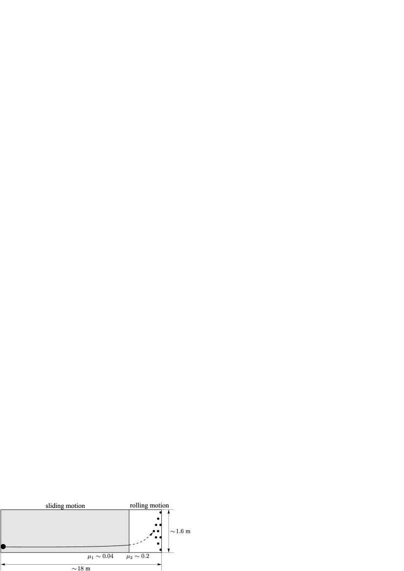
Figure 1: Scheme of bowling. Oiled path of sliding (the solid line) and rough path of rolling (the dashed line) of a ball.

While the first stage is a well known effect of motion of a ball in a parabola during sliding, studied by Euler [11], the second stage is a more complex motion studied in a large body of literature. It is well known that a homogeneous ball rolls in a straight line [5], this fact is also illustrated with bowling [12]. But this effect can be observed in unprofessional amateur bowling, where paths and balls are not prepared in a special way. A great deal of classical research is devoted to the dynamics of a ball with nonuniform mass distribution [6, 9], where it is shown that the trajectory of a ball deviates from a straight line during the rolling motion. Some papers are directly concerned with explanation and prediction of the dynamics of special professional bowling balls [13, 14] with emphasis on the final instant of the ball’s motion — hook.

However, as stated above, the ball starts a curl at the stage of sliding. This curling depends on the coefficient of friction. The question arises whether we can can we reach the effect of hook on the stage of sliding before the transition to rolling, for example, when the ball passes from the smoother to the rougher surface of the path. It is also of interest to consider a more complicated problem of a sliding ball. Assuming the coefficient of friction to be variable, we could calculate the boundary between the surfaces in the path in such a way that parallel families of trajectories of sliding analogous balls with equal initial conditions (linear and angular velocities) converges to a predetermined point, for example, to the central skittle in the bowling (fig. 2). We call this phenomenon — the effect of “mechanical lens” by analogy with the optical effect of the well known collecting lens focusing the light beams in one point.

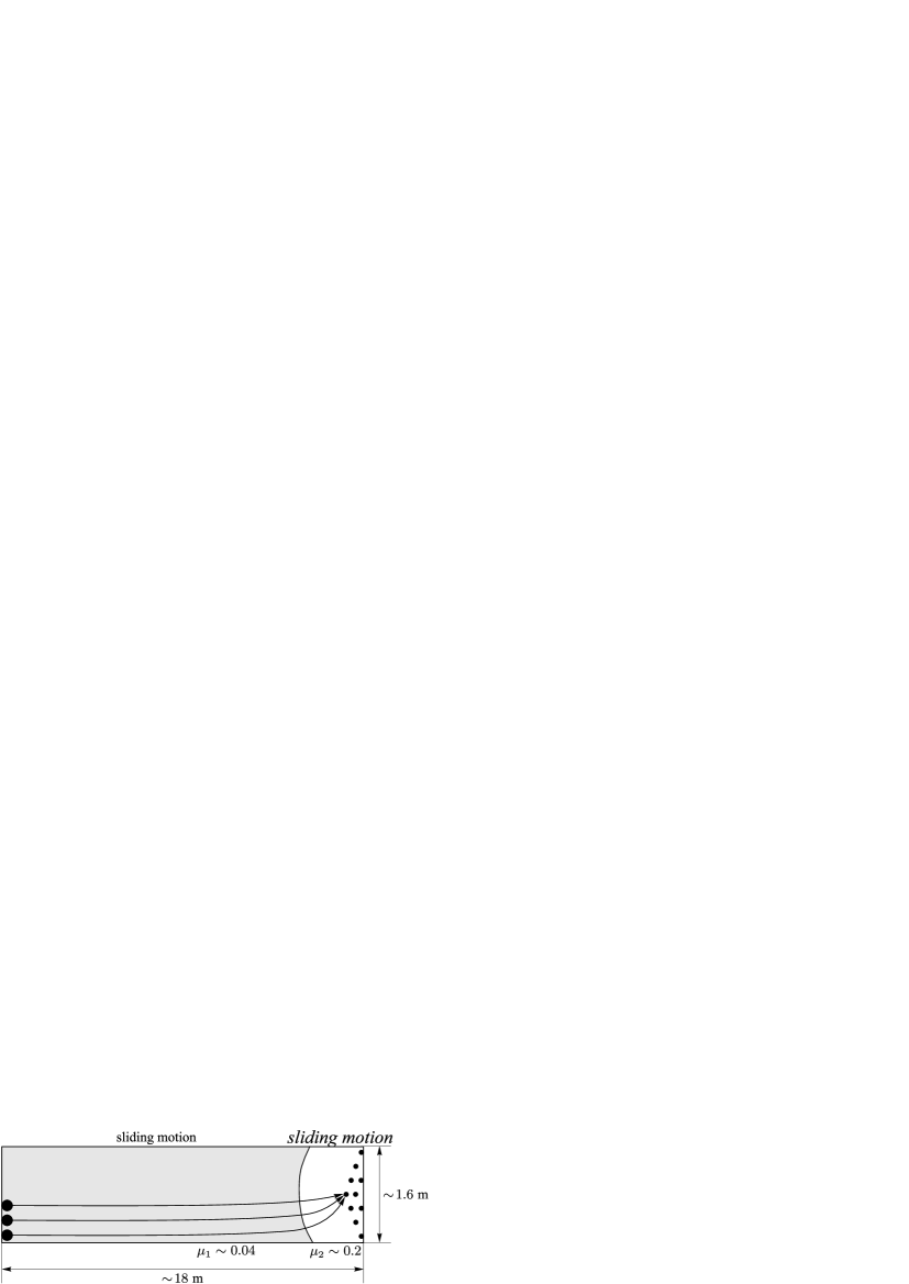
Figure 2: Scheme of a “mechanical lens” in bowling. The balls slide from the starting points till the target point without rolling.

Thus, this paper is devoted to analytical and numerical studies of the effect of the curling of a trajectory and the effect of a “mechanical lens” in the dynamics of a ball during sliding. Also, we study a possible application of these phenomena to the bowling game.

2 Equations of motion of a sliding ball

Consider a heavy homogeneous ball moving by inertia on a fixed rough horizontal plane. We assume the velocity of the point of contact to be sufficiently large to neglect the spinning friction and rolling friction and their influence on the law of sliding friction. For the latter we take the Coulomb formula

$$\boldsymbol{F}=-\mu P\frac{\boldsymbol{u}}{u},$$ (1)

where $\boldsymbol{F}$ is the friction force, $P$ is the weight of the ball, $\mu$ is the coefficient of friction and $\boldsymbol{u}$ is the velocity of the point of contact. This system was first investigated in 1758 by Johann Euler (a son of Leonhard Euler) [11]. We list the basic properties of motion which are important in what follows.

1. $\boldsymbol{e}=\frac{\boldsymbol{u}}{u}=\mbox{const}$, i.e. the direction of sliding does not change;

2. if the initial velocity of the center of the ball $\boldsymbol{v}_{0}$ is not collinear to $\boldsymbol{e}=\frac{\boldsymbol{u}}{u}$, then the center of the ball moves in a parabola (until the ball stops sliding)

   $$\boldsymbol{r}=\boldsymbol{r}_{0}+\boldsymbol{v}_{0}t+\frac{1}{2}ft^{2}\boldsymbol{e},\quad f=\mu g,$$ (2)

   where $\boldsymbol{r}$ is the radius vector of the point of contact, $\boldsymbol{r}_{0}$ is its initial value (for $t=0)$, $t$ is the duration of the motion and $g$ is the free-fall acceleration;

3. The absolute value of the sliding velocity decreases by the law

   $$u=u_{0}-f\left({1+\frac{R^{2}}{\rho^{2}}}\right)t,$$ (3)

   where $u_{0}$ is the initial value and $R$ and $\rho$ are the radius of the ball and its radius of inertia, respectively.

These properties allow the trajectory of the center of the ball to be uniquely constructed.

Using equations (2) and (3) it is not difficult to show qualitative and quantitative changes of trajectories of a sliding ball during the passage from the smoother to the rougher surface of the path. In Figure 3 the families of trajectories of a sliding bowling ball with different initial linear and angular velocities are shown. At the points $r_{i}$ the coefficient of friction changes from $\mu_{1}=0.04$ to $\mu_{2}=0.06$, $\mu_{3}=0.8$, $\mu_{4}=0.1$, $\mu_{5}=0.5$. As evident from Fig. 3 the growth of the coefficient of friction leads to an earlier termination of the sliding motion of the ball and to a more significant curling of its trajectory. It is also clear that both quantities strongly depend on initial conditions of the system.

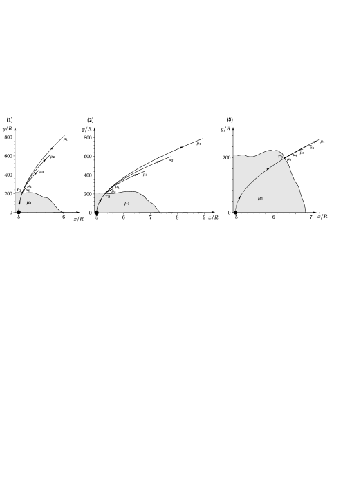
Figure 3: Deviation of three families of trajectories of a sliding bowling ball from a straight line during the sliding motion when the coefficient of friction changes from $\mu_{1}=0.04$ to different values: $\mu_{2}=0.06$, $\mu_{3}=0.08$, $\mu_{4}=0.1$, $\mu_{5}=0.5$. The mass and radius of a ball are $m=5$ kg, $R=0.1$ m, respectively. For the first family (1) of trajectories the initial linear and angular velocities are $\boldsymbol{v_{0}}=[0;10]$ m/s, $\boldsymbol{w_{0}}=[0;1]$ s^-1, for the second (2) $\boldsymbol{v_{0}}=[0;10]$ m/s, $\boldsymbol{w_{0}}=[3;4]$ s^-1, for the third (3) $\boldsymbol{v_{0}}=[0;6]$ m/s, $\boldsymbol{w_{0}}=[5;5]$ s^-1.

Assuming $u=0$ in (3), it not difficult to define the time of sliding of the ball on the surface with the coefficient of friction $\mu$

$$t=\frac{2u_{0}}{7\mu g}$$

and to estimate it for different couples of surfaces. For example, for the family (1) the total time of sliding is $t=2.41$ sec for the couple $(\mu_{1};\mu_{5})$, whereas if the ball slides on a homogeneous surface with $\mu_{1}$, the total time is $t=7.14$ sec.

3 Equation of the boundary curve between two surfaces

Now assume that the coefficient of friction is variable. Let us calculate the boundary between the surfaces on the path in such a way that parallel families of analogous homogenous sliding balls launched under equal initial conditions (linear and angular velocities) on a horizontal rough plane converge to a predetermined point. Let us write the analytical equation for the curve that is the boundary between the surfaces.

Let us choose a starting segment $[AB]$ (without loss of generality we set $[AB]\in Ox$) and assume that for all trajectories emanating from it the vectors $\boldsymbol{v}_{0}$ and $\boldsymbol{e}$ are equal and noncollinear (see Fig. 4). According to formula (2), at $t>0$ this segment moves uniformly. We take the dependence of the coefficient of friction on $\boldsymbol{r}$ to be binary, i.e.

$$f\left({\boldsymbol{r}}\right)=\left\{\begin{aligned} &f_{1},&&\mbox{if}\quad\varphi\left({\boldsymbol{r}}\right)<0\\ &f_{2},&&\mbox{if}\quad\varphi\left({\boldsymbol{r}}\right)\geq 0\end{aligned}\right.$$ (4)

where $f_{1}\neq f_{2}$ and the function $\varphi\left({\boldsymbol{r}}\right)$ specifying the boundary curve between two surfaces for $\varphi\left({\boldsymbol{r}}\right)=0$ must be defined.

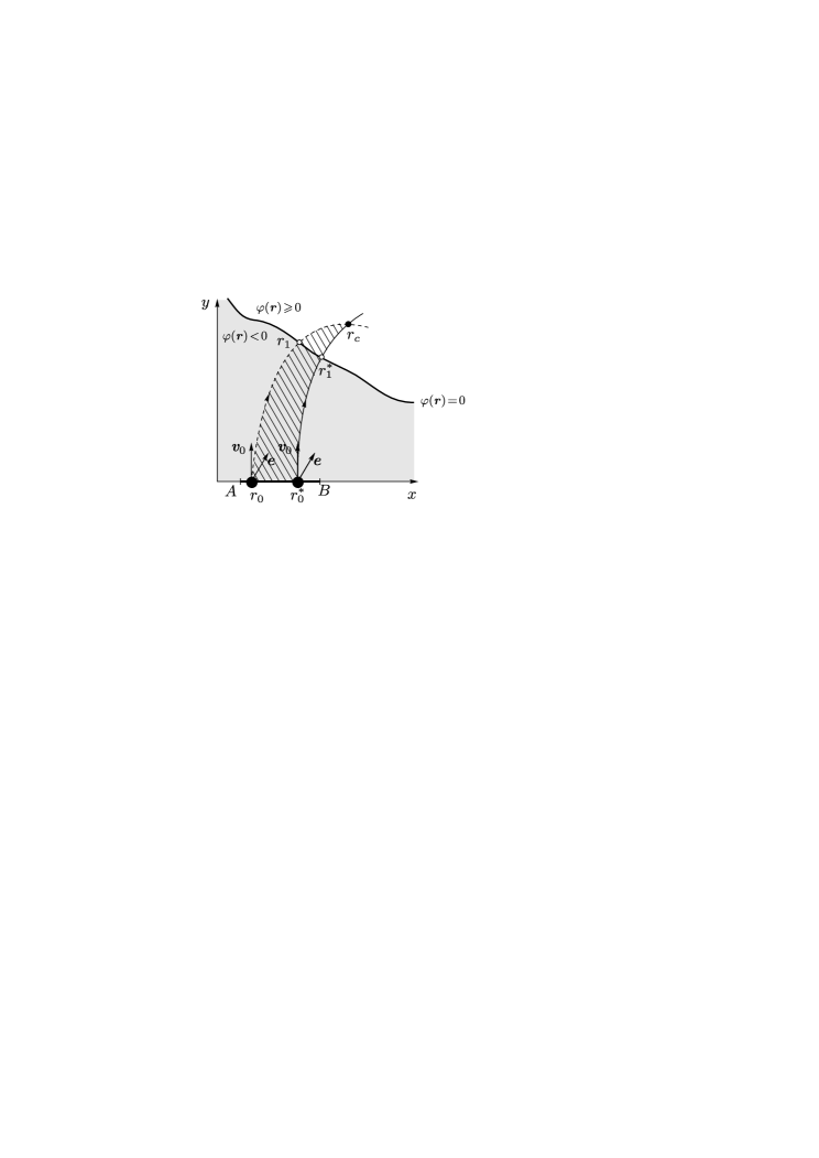
Figure 4: Scheme of the model of “mechanical lens”. The curve $\varphi\left({\boldsymbol{r}}\right)=0$ corresponds to the boundary curve between two surfaces. The shaded area is a domain of attraction of the system.

Let us take a point $\boldsymbol{r}_{0}^{\ast}$ from the interval $(AB)$ as the initial value and construct the trajectory (2) emanating from it. We shall assume this trajectory to be supporting and choose on it a target point $C$ which must be reached by all trajectories sufficiently close to this one. To do this, we fix two quantities: $t_{1}>0$ is the time of motion in the region $\varphi\left({\boldsymbol{r}}\right)<0$ and $s>0$ is the time of motion in the region $\varphi\left({\boldsymbol{r}}\right)>0$. Such a choice is sufficiently arbitrary, we only need to make sure (formula (3)) that the friction has no time to stop the sliding motion of the ball. In addition, the quantity $t_{1}$ should not be small, since otherwise the boundary curve between two surfaces can cross the starting segment, which will narrow the family of balls. Due to (2) and (4) the equation of the supporting trajectory is

$$\begin{gathered}\boldsymbol{r}^{\ast}(t)=\left\{\begin{aligned} &\boldsymbol{r}_{0}^{\ast}+\boldsymbol{v}_{0}t+\frac{1}{2}f_{1}t^{2}\boldsymbol{e},&&\text{if}\quad t\leq t_{1}\\ &\boldsymbol{r}_{1}^{\ast}+\boldsymbol{v}_{1}^{\ast}(t-t_{1})+\frac{1}{2}f_{2}(t-t_{1})^{2}\boldsymbol{e},&&\mbox{if}\quad t_{1}\leq t\leq t_{1}+s\\ \end{aligned}\right.\\ \boldsymbol{r}_{1}^{\ast}=\boldsymbol{r}_{0}^{\ast}+\boldsymbol{v}_{0}t_{1}+\frac{1}{2}f_{1}t_{1}^{2}\boldsymbol{e},\quad\boldsymbol{v}_{1}^{\ast}=\boldsymbol{v}_{0}+f_{1}t_{1}\boldsymbol{e}.\end{gathered}$$ (5)

The radius vector of the target point $\boldsymbol{r}_{C}$ is defined from the formula

$$\boldsymbol{r}_{C}=\boldsymbol{r}_{1}^{\ast}+\left({\boldsymbol{v}_{0}+f_{1}t_{1}\boldsymbol{e}}\right)s+\frac{1}{2}f_{2}s^{2}\boldsymbol{e},$$ (6)

and the boundary curve between two surfaces passes through the point $\boldsymbol{r}_{1}^{\ast}$, i.e. $\varphi\left({\boldsymbol{r}_{1}^{\ast}}\right)=0$.

We now consider another trajectory from this family. Its initial point $\boldsymbol{r}_{0}$ in the interval $(AB)$ is defined by the number $\delta$ (proportional to the distance between $\boldsymbol{r}_{0}^{\ast}$ and $\boldsymbol{r}_{0})$, so that

$$\boldsymbol{r}_{0}=\boldsymbol{r}_{0}^{\ast}+\delta\boldsymbol{i}=\boldsymbol{r}_{0}^{\ast}+\delta(\alpha\boldsymbol{v}_{0}+\beta\boldsymbol{e}),$$ (7)

where $\alpha,\beta$ are the coordinates of the direction vector $\boldsymbol{i}$ of the straight line $(AB)$ in the skew-angular basis $(\boldsymbol{v}_{0},\;\boldsymbol{e})$. By analogy with (5), the equation of this trajectory is

$$\begin{gathered}\boldsymbol{r}(t)=\left\{\begin{aligned} &\boldsymbol{r}_{0}+\boldsymbol{v}_{0}t+\frac{1}{2}f_{1}t^{2}\boldsymbol{e},&&\mbox{if }t\leq t_{1}+\tau\\ &\boldsymbol{r}_{1}+\boldsymbol{v}_{1}(t-t_{1}-\tau)+\frac{1}{2}f_{2}(t-t_{1}-\tau)^{2}\boldsymbol{e},&&\mbox{if }t_{1}+\tau\leq t\leq t_{1}+\tau+p\\ \end{aligned}\right.\\ \boldsymbol{r}_{1}=\boldsymbol{r}_{0}+\boldsymbol{v}_{0}(t_{1}+\tau)+\frac{1}{2}f_{1}(t_{1}+\tau)^{2}\boldsymbol{e},\quad\boldsymbol{v}_{1}=\boldsymbol{v}_{0}+f_{1}(t_{1}+\tau)\boldsymbol{e},\end{gathered}$$ (8)

where $\boldsymbol{r}_{0}$ is defined by (7), the instant of time $t_{1}+\tau$ corresponds to the intersection of the trajectory with the boundary curve between two surfaces, and the quantity $p$ is equal to the time of motion of the ball in the region $\varphi>0$.

The condition for the trajectory to reach the point $C$ is expressed by the equality

$$\boldsymbol{r}(t_{1}+\tau+p)=\boldsymbol{r}_{C}$$ (9)

The vector equality (9) is equivalent to the system of two scalar equations in two unknowns, $\tau$ and $p$, which also contains the parameter $\delta$ defining the initial position of the trajectory from the family. Hence, one can express two of these quantities as some functions of the third one (e.g., $p$ and $\delta$ in terms of $\tau)$. Then the formula

$$\boldsymbol{r}=\boldsymbol{r}_{1}=\boldsymbol{r}_{1}^{\ast}+\delta(\alpha\boldsymbol{v}_{0}+\beta\boldsymbol{e})+\boldsymbol{v}_{0}\tau+\frac{1}{2}f_{1}(2t_{1}\tau+\tau^{2})\boldsymbol{e}$$ (10)

is a parametric equation of the boundary curve between two surfaces. In particular, if $\tau=0$ and $\delta=0$, we obtain $\boldsymbol{r}=\boldsymbol{r}_{1}^{\ast}$, which corresponds to the switching point on the supporting curve (5). Consequently, the formula (10) solves the problem.

All trajectories starting from the $\delta$-neighborhood of $\boldsymbol{r}_{0}^{\ast}$ with initial conditions $(\boldsymbol{v}_{0},\;\boldsymbol{e})$ and reaching the target point $\boldsymbol{r}_{C}$ generate the domain of attraction of the system (see Fig. 4).

Remark.

After constructing the boundary curve between two surfaces (10), we have to make sure that the supporting trajectory (5) crosses it: in some degenerate cases, touching with return into the region $\varphi<0$ is possible. In addition, it is necessary to make sure that there are no repeated intersections with these lines.

Substituting (6), (7) and (10) in (9), we obtain

$$\begin{gathered}\delta(\alpha\boldsymbol{v}_{0}+\beta\boldsymbol{e})+\boldsymbol{v}_{0}\tau+\frac{1}{2}f_{1}(2t_{1}\tau+\tau^{2})\boldsymbol{e}++\left({\boldsymbol{v}_{0}+f_{1}\left({t_{1}+\tau}\right)\boldsymbol{e}}\right)p+\frac{1}{2}f_{2}p^{2}\boldsymbol{e}=\\ =\left({\boldsymbol{v}_{0}+f_{1}t_{1}\boldsymbol{e}}\right)s+\frac{1}{2}f_{2}s^{2}\boldsymbol{e}.\end{gathered}$$ (11)

Equating the coefficients for the basis vectors $\boldsymbol{v}_{0}$ and $\boldsymbol{e}$ on the left-hand and right-hand sides of (11), we obtain the system

$$\alpha\delta+\tau+p=s,$$ (12)

$$\beta\delta+f_{1}t_{1}\tau+\frac{1}{2}f_{1}\tau^{2}+f_{1}(t_{1}+\tau)p+\frac{1}{2}f_{2}p^{2}=f_{1}t_{1}s+\frac{1}{2}f_{2}s^{2}.$$ (13)

Eq. (12) is linear and allows us to eliminate one of the variables without difficulty. Eq. (13) is quadratic, and it takes extra effort to use it.

4 The case of an absolutely smooth surface on one of the phases of motion

We point out two limiting particular cases where Eq. (13) simplifies.

• $\boldsymbol{f_{1}=0}$, $\boldsymbol{f_{2}\neq 0}$, i. . the ball moves first on the smooth part of the plane (“ice”) and then gets onto the rough part.

  Eq. (13) becomes

  $$\beta\delta+\frac{1}{2}f_{2}p^{2}=\frac{1}{2}f_{2}s^{2}.$$

  If $\beta\neq 0$ (i.e. the starting segment $[AB]$ is not collinear to the initial velocity $\boldsymbol{v}_{0})$, then

  $$\delta=\frac{1}{2}\beta^{-1}f_{2}\left({s^{2}-p^{2}}\right),\quad\tau=s-\alpha\delta-p.$$

  In (10) we obtain a parametric equation of the boundary curve between two surfaces in the form

  $$\boldsymbol{r}(p)=\boldsymbol{r}_{1}^{\ast}+\delta(\alpha\boldsymbol{v}_{0}+\beta\boldsymbol{e})+\tau\boldsymbol{v}_{0}=\boldsymbol{r}_{1}^{\ast}+\frac{1}{2}f_{2}\left({s^{2}-p^{2}}\right)\boldsymbol{e}+(s-p)\boldsymbol{v}_{0},$$ (14)

  where $\delta=0$ and $\boldsymbol{r}=\boldsymbol{r}_{1}^{\ast}$ correspond to the value of the parameter $p=s$, i.e. we are on the supporting curve. Eq. (14) defines the curve of order 2, which is obviously a parabola, since it is unbounded and connected.

  In the case $\beta=0$ all trajectories emanating from the segment $\left[{AB}\right]$ merge to form a single (supporting) trajectory, although the switching point $\boldsymbol{r}_{1}^{\ast}$ is reached at different instants of time.

• $\boldsymbol{f_{1}\neq 0,\;f_{2}=0}$, i.e. the ball moves first on the rough part of the plane and then gets onto “ice”.

  Eq. (13) becomes

  $$\beta\delta+f_{1}t_{1}\tau+\frac{1}{2}f_{1}\tau^{2}+f_{1}(t_{1}+\tau)p=f_{1}t_{1}s.$$

  Substituting (12) into the above equation gives

  $$\delta\left({\beta-\alpha f_{1}(t_{1}+\tau)}\right)-\frac{1}{2}f_{1}\tau^{2}+f_{1}\tau s=0.$$ (15)

  In this case it is more convenient to use $\tau$ as a parameter. If

  $$\beta-\alpha f_{1}t_{1}\neq 0,$$ (16)

  then the coefficient with $\delta$ in (15) is different from zero in a sufficiently small neighborhood of the value $\tau=0$. Then

  $$\delta=f_{1}\tau\left({\frac{1}{2}\tau-s}\right)\left({\beta-\alpha f_{1}(t_{1}+\tau)}\right)^{-1}.$$ (17)

  Substituting (17) in (10), we obtain a representation of the boundary curve between two surfaces in the form of a rational parametric curve

  $$\boldsymbol{r}(\tau)=\boldsymbol{r}_{1}^{\ast}+f_{1}\tau\left({\frac{1}{2}\tau-s}\right)\left({\beta-\alpha f_{1}(t_{1}+\tau)}\right)^{-1}(\alpha\boldsymbol{v}_{0}+\beta\boldsymbol{e})+\boldsymbol{v}_{0}\tau+\frac{1}{2}f_{1}(2t_{1}\tau+\tau^{2})\boldsymbol{e},$$

  Note that the value $\tau=0$ corresponds to the supporting trajectory.

  In the case where an equality takes place in formula (16), (15) becomes

  $$f_{1}\tau\left({\delta\alpha-\frac{1}{2}\tau+s}\right)=0.$$

  This means that either $\tau=0$ and $\delta$ is arbitrary, or $\delta\alpha-\frac{1}{2}\tau+s=0$. In the former case, formula (10) describes a segment parallel to the starting segment $[AB]$. However, it turns out that when the boundary curve between two surfaces is reached the trajectory touches this curve, and then all trajectories pass along the switching segment, the target point $C$ also lies on this segment.

  In the latter case, $\alpha\neq 0$, otherwise by virtue of the equality opposite to (16), we would also have $\beta=0$, which is impossible, since $\boldsymbol{i}\neq 0$. Hence, $\delta$ will be a linear function of $\tau$, and the formula (10) describes a parabola (by analogy with the case $1^{\circ}$). However, such a curve does not contain the point of the supporting trajectory $\tau=0$, $\delta=0$. Therefore, it cannot be regarded as a solution to the problem.

5 Analysis of motion in the general case

We now turn to a discussion of the general case $0<f_{1}\neq f_{2}>0$. By using (12) twice, we bring (13) to the form

$$\delta(\beta-f_{1}t_{1})+\frac{1}{2}f_{1}(\alpha^{2}\delta^{2}-2\alpha\delta s)+\frac{1}{2}\left({f_{2}-f_{1}}\right)p^{2}=\frac{1}{2}\left({f_{2}-f_{1}}\right)s^{2},$$

whence

$$p(\delta)=\left[{s^{2}-\left({2\delta(\beta-\alpha f_{1}t_{1})+f_{1}(\alpha^{2}\delta^{2}-2\alpha\delta s)}\right)\left({f_{2}-f_{1}}\right)^{-1}}\right]^{1/2}.$$ (18)

The sought-for curve is irrational. It is governed by the formula

$$\boldsymbol{r}(\delta)=\boldsymbol{r}_{1}^{\ast}+\delta(\alpha\boldsymbol{v}_{0}+\beta\boldsymbol{e})+\boldsymbol{v}_{0}\tau+\frac{1}{2}f_{1}(2t_{1}\tau+\tau^{2})\boldsymbol{e},$$ (19)

$$\tau=s-p(\delta)-\alpha\delta,$$

where $p(\delta)$ is expressed by (18). We note that for $\delta=0$ we have $p=s$ and $\tau=0$, which corresponds to the supporting trajectory.

We make sure that the curve (19) intersects the supporting trajectory, i.e. the vector $\boldsymbol{v}_{1}^{\ast}=\boldsymbol{v}_{0}+f_{1}t_{1}\boldsymbol{e}$ is not tangential to this curve. The tangent vector to the curve (19) at the point of its intersection with the supporting trajectory is defined by the formula

$$\left.{\frac{d\,\boldsymbol{r}(\delta)}{d\,\tau}}\right|_{\tau=0}=\left.{\frac{d\,\delta}{d\,\tau}}\right|_{\tau=0}(\alpha\boldsymbol{v}_{0}+\beta\boldsymbol{e})+\boldsymbol{v}_{0}+f_{1}t_{1}\boldsymbol{e}.$$ (20)

It follows from (18) and (19) that the derivative on the right-hand side of (20) is different from zero under the condition $p\neq 0$, which is obviously satisfied in a neighborhood of the supporting trajectory (on which $p=s)$. Consequently, the no-touching condition is equivalent to the non-collinearity of the vectors $\boldsymbol{v}_{1}^{\ast}$ and $\boldsymbol{i}=\alpha\boldsymbol{v}_{0}+\beta\boldsymbol{e}$, i.e.

$$\beta\neq\alpha f_{1}t_{1}.$$ (21)

We note that the condition (21) is equivalent to (16).

Summarizing the investigation, we formulate the main result in the form of a theorem.

Theorem 1.

Suppose there is a family of balls which is characterized by the initial velocity of the center $\boldsymbol{v}_{0}$ and by the unit vector opposing the sliding velocity of the point of contact $\boldsymbol{e}$, and positive coefficients of friction $\mu_{1}\neq\mu_{2}$. The initial positions of the points of contact lie on the segment of a straight line with the direction vector $\boldsymbol{i}=\alpha\boldsymbol{v}_{0}+\beta\boldsymbol{e}$. Let one of the trajectories emanating from this segment be the supporting trajectory. The motion along the supporting trajectory consists of two phases (see (5)). The duration of the first phase $t_{1}$ is determined according to (21). The target point $C$ lies on the supporting trajectory and is determined by the duration of the second phase $s$ whose value is limited by the sliding condition (in the formula (3) $u>0)$.

Then there exists a unique boundary curve between two surfaces during the intersection with which the coefficient of friction changes from $\mu_{1}$ to $\mu_{2}$, such that for sufficiently small $|\delta|$ all trajectories of the family pass through the point $C$.

An analogous assertion holds in the limiting cases $\mu_{1}=0$ (under the condition $\beta\neq 0)$ and $\mu_{2}=0$. If $\mu_{1}=0,\,\beta=0$, then all trajectories merge into a single one (with time shift), and the boundary curve between two surfaces is not determined.

6 Examples of focusing trajectories of a sliding balls

Using the above algorithm, we construct the curves of the boundary between the surfaces (19), supporting trajectories (6) of a sliding ball and trajectories from its $\delta$-neighborhood (8) for different couples of surfaces: for the cases of a passage to the smoother or to the rougher plane.

Set the initial segment $[AB]\in Ox$, the initial values of velocities of the ball $\boldsymbol{v}_{0}=5\boldsymbol{j}$, $\boldsymbol{e}=\frac{1}{2}\boldsymbol{i}+\frac{\sqrt{3}}{2}\boldsymbol{j}$, the coefficient of friction of the surface in the first phase of motion $\mu_{1}=0.2$ and suppose that the supporting trajectory emanates from the point $\boldsymbol{r_{0}}^{*}=\boldsymbol{i}$. Construct the trajectory and calculate the corresponding time $t$ of the motion of the ball until complete stop assuming that the entire surface is homogeneous with $\mu_{1}=0.2$. Construct a supporting curve according to (5). Choose on the trajectory the point $\boldsymbol{r}_{1}^{*}(t_{1}<t)$ at which the value of the friction coefficient changes from $\mu_{1}$ to $\mu_{2}$. Define on the trajectory of the second phase of motion the target point $\boldsymbol{r}_{C}(s)$ through which all trajectories emanating from the $\delta$-neighborhood of the point $\boldsymbol{r}_{0}^{*}$ must pass. Construct according to (19) the boundary curve between two surfaces and the trajectories of motion of balls sufficiently close to the supporting one. :

1. Set $\mu_{2}=0.1$, i.e. the ball passing through the boundary between the two surfaces reaches the smoother surface. For this case the supporting trajectory, the target point, boundary curve between two surfaces, the trajectories of the family and the domain of attraction are shown in Fig. 5. The curve of the boundary between the two surfaces has the form of a convex lens, and the $\delta$-neighborhood (domain of attraction) which the trajectories leave before converging to a target point is about $0.007$ meters.

2. Set $\mu_{2}=0.5$, i.e. the ball passing through the boundary between the two surfaces reaches the rougher surface. The supporting curve, the target point, the boundary curve between two surfaces, the trajectories of the family and the domain of attraction are shown in Fig. 6. The curve of the boundary between two surfaces has the form of a slightly concave lens, and the $\delta$-neighborhood (domain of attraction) which the trajectories leave before converging to a target point is about $0.001$ meters.

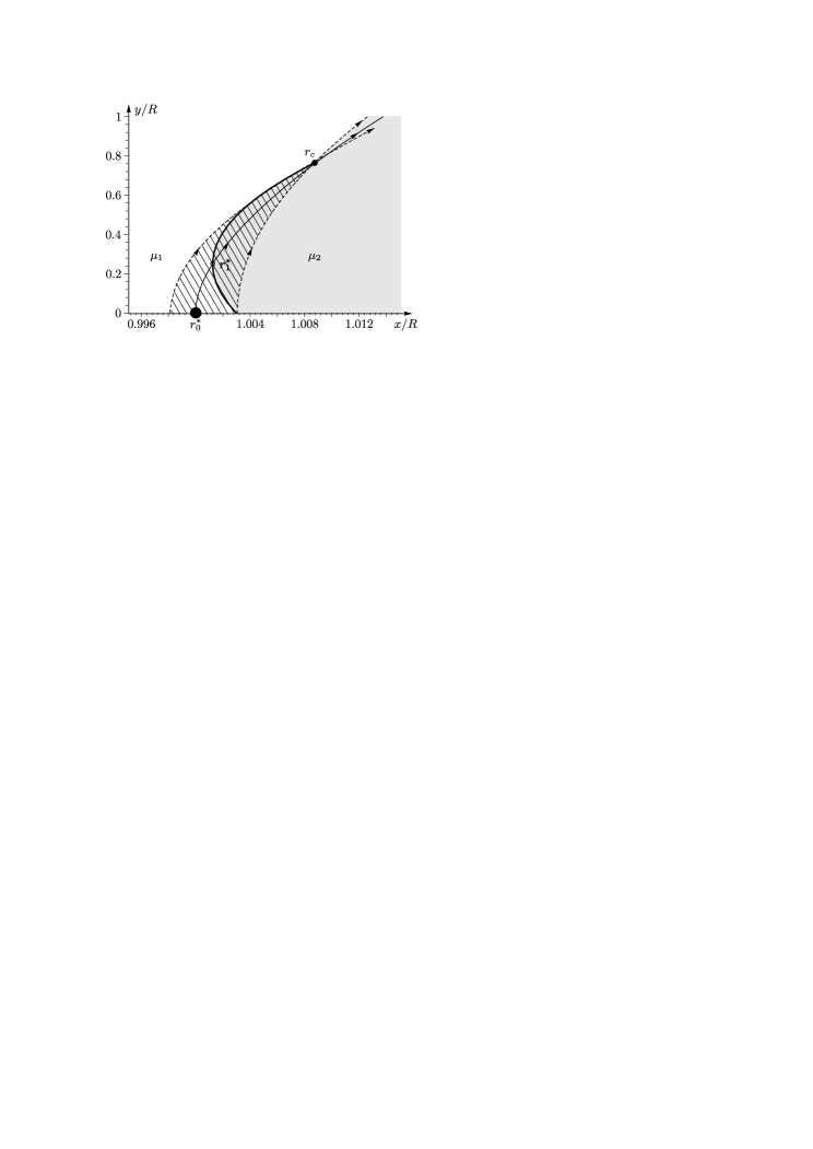
Figure 5: Supporting trajectory (thin solid line), the curve of the boundary between two surfaces (thick solid line), the point of boundary between two surfaces on the supporting trajectory $\boldsymbol{r}_{1}^{*}$, the target point $\boldsymbol{r}$ and a couple of trajectories from a family (dashed lines) for the case $\mu_{1}=0.2$, $\mu_{2}=0.1$. The shaded area is a domain of attraction of the system.

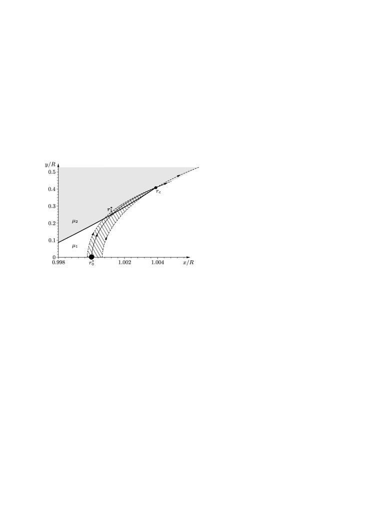
Figure 6: Supporting trajectory (thin solid line), the curve of boundary between two surfaces (thick solid line), the point of boundary between two surfaces on the supporting trajectory $\boldsymbol{r}_{1}^{*}$, the target point $\boldsymbol{r}$ and a couple of trajectories from a family (dashed lines) for the case $\mu_{1}=0.2$, $\mu_{2}=0.5$. The shaded area is a domain of attraction of the system.

The case of bowling balls

Now consider the dynamics of a system similar to the system of a sliding ball in bowling. Set $m=1$ kg, $R=0.1$ m, $\mu_{1}=0.04$, $\mu_{2}=0.2$, $\boldsymbol{v_{0}}=[0;10]$ m/s, $\boldsymbol{\omega_{0}}=[0;5]$ s^-1, $\boldsymbol{r_{0}}^{*}=0.8$ m. We can calculate the values $u_{0}\approx 10$ m/s and $\boldsymbol{e}\approx 0.05\boldsymbol{i}+0.1\boldsymbol{j}$. Let us construct a supporting trajectory and choose the time of motion on different surfaces so that the target point $\boldsymbol{r_{C}}$ coincides with the position of the central skittle. Further, let us construct the curve of boundary between two surfaces and the trajectories of motion of the balls leaving the $\delta$-neighborhood (domain of attraction) and converging to the target point (see Fig. 7). The calculations have shown that the boundary between the two surfaces has the form of a slightly concave lens as in the previous case. The $\delta$-neighborhood which the trajectories leave before converging to the target point is about $0.05$ meters. The other trajectories from the $\delta$-neighborhood don’t reach the target point since the sliding motion terminates earlier.

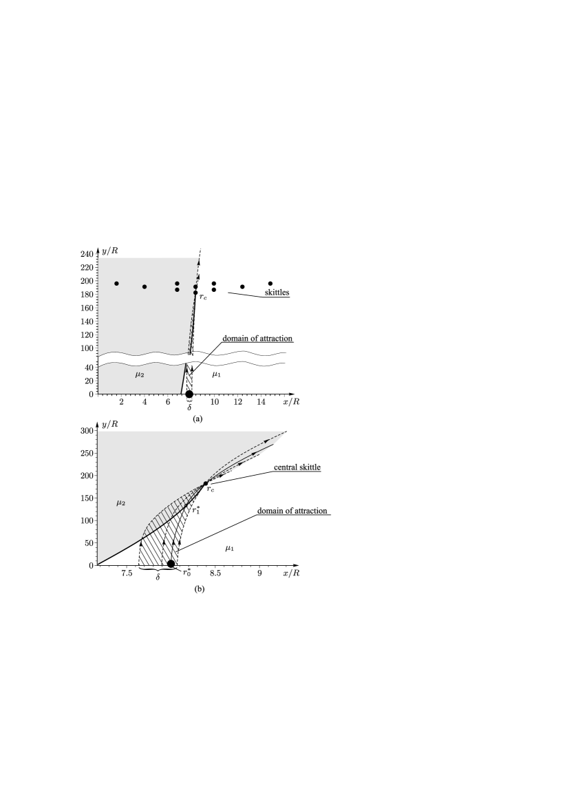
Figure 7: The system similar to the system of a sliding ball in bowling in two different scales: (a) the scale that is closer to the real bowling system, (b) the scale with an increased and more detailed domain of attraction. The thin solid line is the supporting trajectory, the thick solid line is the curve of the boundary between two surfaces is , $\boldsymbol{r}_{1}^{*}$ is the point of the boundary between two surfaces on the supporting trajectory and $\boldsymbol{r}$ is the target point. The dashed lines are the trajectories from a family, the shaded area is a domain of attraction of the system. The coefficients of friction are $\mu_{1}=0.04$, $\mu_{2}=0.2$, and the initial velocities are $\boldsymbol{v_{0}}=[0;10]$ m/s, $\boldsymbol{\omega_{0}}=[0;5]$ s^-1.

7 Discussion

Assuming the coefficient of friction to be variable, we have presented the algorithm and constructed the curves of the boundary between two surfaces on a plane in such a way that parallel families of analogous homogenous sliding balls launched under equal initial conditions (linear and angular velocities) on a horizontal rough plane, converges to a predetermined point. Calculations are presented for some arbitrary cases of passage to the smoother or to the rougher surface, and also for a system similar to that of a sliding ball in bowling before the transition to rolling.

Numerical experiments have shown that the relations between the s of the initial positions of the balls in the families and dimensions of a sliding domain are very small, and the curves of the boundary between two surfaces for the cases of passage to the smoother or to the rougher surface have qualitative differences.

For example, for the family of balls passing during sliding to the smoother surface (see Fig. 5), the curve of the boundary between two surfaces leaves the abscissa axis on the right of the supporting trajectory and reaches the target point above the supporting trajectory and has the form of a convex lens. For the family passing during sliding to the rougher surface (see Fig. 6), the curve of the boundary between two surfaces leaves the abscissa axis on the left of the supporting trajectory and reaches the target point below the supporting trajectory and has the form of a slightly concave lens.

As for possible application of this effect of refraction of trajectories for the bowling game, it seems that a novice player has to train hard at first to inscribe the ball into a small $\delta$-neighborhood of the starting point of the supporting trajectory and to impart the required initial velocities to the ball. Also, it is clear that the dimensions of the domain of attraction ($\delta$-neighborhood) are rather small, about $5$ cm (see Fig. 7).

It should be noted that the model considered can be applicable under quite rare conditions of the ball’s motion — pure sliding without rolling. Incorporating the rolling motion adds the realism to the system, but implies consideration of more complicated model, for example, the nonholonomic model extensively studied in [10], particular motion in the limiting case of passage of the ball from an absolutely rough to an absolutely smooth surface is considered in [15].

8 Appendix. Estimate of possible dimensions of domain of attraction

One way to enlarge the domain of attraction is to increase the number of the curves of a boundary between surfaces $\varphi(r)$ in (8). Physically this can be done by gluing figured strips from materials with different coefficients of friction onto the floor. The form of these strips can be calculated by analogy with Sections 2–5. It should be kept in mind that, in contrast to the case of a single switching, the form of the strips is not uniquely defined by the condition (9), and it is necessary to add some optimization requirement, which complicates the problem significantly.

An estimate of the maximum of the domain of attraction can be found by considering the family of parabolas (7) and (8) without switching. Each of the parabolas is characterized by its coefficient of friction $f(\delta)$, which corresponds to a continuous change of the coefficient of friction on the supporting plane. The boundary values for the initial conditions $\left({\delta_{\min},\delta_{\max}}\right)$ correspond to the limiting values

$$f(\delta_{\min})=f_{\max},\quad f(\delta_{\max})=0,$$

where the value $f_{\max}$ corresponds to the maximally rough material used. We define the target point $C$ as the intersection of the limit trajectories

$$\boldsymbol{r}_{0}^{\ast}+\delta_{\max}\boldsymbol{i}+\boldsymbol{v}_{0}t_{1}=\boldsymbol{r}_{C},\quad\boldsymbol{r}_{0}^{\ast}+\delta_{\min}\boldsymbol{i}+\boldsymbol{v}_{0}t_{2}+\frac{1}{2}f_{\max}t_{2}^{2}\boldsymbol{e}=\boldsymbol{r}_{C},$$ (22)

where $\delta_{\min}$ and $t_{2}$ are given arbitrarily, and $\delta_{\max}$ and $t_{1}$ are found from the vector equality

$$\left({\delta_{\max}-\delta_{\min}}\right)(\alpha\boldsymbol{v}_{0}+\beta\boldsymbol{e})+\boldsymbol{v}_{0}t_{1}=\boldsymbol{v}_{0}t_{2}+\frac{1}{2}f_{\max}t_{2}^{2}\boldsymbol{e}.$$ (23)

For the values $\delta\in\left({\delta_{\min},\delta_{\max}}\right)$ the quantity $f(\delta)$ is chosen such that the parabola (8) with this coefficient crosses the target point. Thus, the lines of the level set of the function $f$ on the supporting plane have the form of parabolas (in the limit $f\to 0$ is a straight line).

Equating the coefficients with $\boldsymbol{e}$ in (23), we obtain

$$\left({\delta_{\max}-\delta_{\min}}\right)\beta=\frac{1}{2}\mu_{\max}gt_{2}^{2}.$$ (24)

Formula (24) shows that the dimension of the domain of attraction is proportional to the maximum coefficient of friction and to the square of time of the motion of a ball into the target point. If we set $\mu=0.3$, $t=4$ seconds, we obtain 24 meters of the maximum possible length of the domain of attraction.

9 Acknowledgements

The authors are grateful to Oliver O’Reilly, Alexey Borisov, Ivan Mamaev and Tatiana Ivanova for useful discussions and valuable remarks. The N. Erdakova’s work was supported by the Grant RFBR 15-08-09261- . The A. Ivanov’s work was supported by the RFBR grant 14-01-00432 and was carried out within the framework of the basic part of the state assignment 2014/120.

References

- [1] Vielsack P. Stick-slip instability of decelerative sliding // International Journal of Non-Linear Mechanics, 2001, vol. 36, no. 2, pp. 237-247
- [2] A.V. Borisov, N.N. Erdakova, T.B. Ivanova, I.S. Mamaev The Dynamics of a Body with an Axisymmetric Base Sliding on a Rough Plane Regular and Chaotic Dynamics, 2014, 19 (6), pp. 607 - 634
- [3] M. Shegelski, R. Niebergall, M. Walton, The motion of a curling rock, Canadian Journal of Physics 74 (9–10) (1996) 663–670.
- [4] A. Ivanov, N. Shuvalov, On the motion of a heavy body with a circular base on a horizontal plane and riddles of curling, Regular and Chaotic Dynamics 17 (1) (2012) 97–104. doi:10.1134/S156035471201008X.
- [5] S. Chaplygin, On a ball’s rolling on a horizontal plane, Regular and Chaotic Dynamics 7 (2) (2002) 131–148.
- [6] N. Zhukovski, On bobylev’s gyroscopic ball, Proceedings of the Physical Sciences’ section of the Society of Amateurs of Natural Sciences VI.
- [7] M. Batista, Steady motion of a rigid disk of finite thickness on a horizontal plane, Int. J. Non-Linear Mech. 41 (4) (2006) 605 621.
- [8] M. Batista, Integrability of the motion of a rolling disk of finite thickness on a rough plane, Int. J. Non-Linear Mech. 41 (6-7) (2006) 850 859.
- [9] A. Borisov, A. Kilin, I. Mamaev, The problem of drift and recurrence for the rolling chaplygin ball, Regular and Chaotic Dynamics 18 (6) (2013) 832–859. doi:10.1134/S1560354713060166.
- [10] A. Borisov, I. Mamaev, The rolling motion of a rigid body on a plane and a sphere. Hierarchy of dynamics, Regular and Chaotic Dynamics 7 (2) (2002) 177–200.
- [11] E. Euler, Recherches plus exactes sur l’effect des moulins à vent, Mem. Acad. Roy. Sci. Berlin 12 (1758) 165–234.
- [12] D. Hopkins, J. Patterson, Bowling frames: Paths of a bowling ball, American Journal of Physics 45 (3) (1977) 263–266.
- [13] C. Frohlich, What makes bowling balls hook?, American Journal of Physics 72 (9) (2004) 1170–1177.
- [14] K. King, N. Perkins, H. Churchill, R. McGinnis, R. Doss, R. Hickland, Bowling ball dynamics revealed by miniature wireless mems inertial measurement unit, Sports Engineering 13 (2) (2011) 95–104.
- [15] J. Cortés, M. de León, D. M. de Diego, S. Martúnez, Mechanical systems subjected to generalized non-holonomic constraints, Proceedings of the Royal Society of London A 457 (2007) (2001) 651–670.