Quantum Discord for $d\otimes 2$ Systems

Abstract

We present an analytical solution for classical correlation, defined in terms of linear entropy, in an arbitrary $d\otimes 2$ system when the second subsystem is measured. We show that the optimal measurements used in the maximization of the classical correlation in terms of linear entropy, when used to calculate the quantum discord in terms of von Neumann entropy, result in a tight upper bound for arbitrary $d\otimes 2$ systems. This bound agrees with all known analytical results about quantum discord in terms of von Neumann entropy and, when comparing it with the numerical results for $10^{6}$ two-qubit random density matrices, we obtain an average deviation of order $10^{-4}$. Furthermore, our results give a way to calculate the quantum discord for arbitrary $n$-qubit GHZ and W states evolving under the action of the amplitude damping noisy channel.

Quantum entanglement plays important roles in many areas of quantum information processing, such as quantum teleportation and superdense coding nielsen ; Horodecki09 ; Guhne09 . Nevertheless, quantum entanglement is not the only form of quantum correlation that is useful for quantum information processing. Indeed, some separable states may also speed up certain quantum tasks, relative to their classical counterparts datta1 ; datta2 ; datta3 ; datta4 , and many quantum tasks, such as quantum nonlocality Horodecki09 ; bennett ; niset and deterministic quantum computations with one qubit Knill , can be carried out with forms of quantum correlation other than quantum entanglement. One such quantum correlation, called quantum discord, has received a great deal of attention recently (see Modi and references therein). Introduced by Ollivier and Zurek ollivier as the difference between the quantum mutual information and the maximal conditional mutual information obtained by local measurements ollivier ; Vedral , quantum discord plays an important role in some quantum information processing ost ; LiB .

Despite much effort by the scientific community, an analytical solution of quantum discord is still lacking even for two-qubit systems. Owing to the maximization involved in the calculation, there are only a few results on the analytical expression of quantum discord and only for very special states are exact solutions known. However, if instead of the von Neumann entropy one uses the linear entropy, the optimal measurements that maximize the conditional mutual information can be obtained analytically osborne . Here, we show that using these optimal measurements to determine the quantum discord in terms of the von Neumann entropy results in an excellent upper bound for the latter. Moreover, we show that this result gives a way to calculate the quantum discord for arbitrary $n$-qubit GHZ and W states, with each qubit subjected to the amplitude damping channel individually.

I Results

I.1 Classical correlation under linear entropy

The usual quantum discord, in terms of von Neumann entropy, is defined as follows: let $\rho^{AB}$ denote the density operator of a bipartite system composed of partitions $A$ and $B$. Let $\rho^{A}=Tr_{B}(\rho^{AB})$ and $\rho^{B}=Tr_{A}(\rho^{AB})$ be the reduced density operators of $A$ and $B$, respectively. The quantum mutual information, which is the information-theoretic measure of the total correlation, is defined as $\mathcal{I}(\rho^{AB})=S(\rho^{A})+S(\rho^{B})-S(\rho^{AB})$, where $S(\rho)=-\rm{Tr}(\rho\log_{2}\rho)$ is the von Neumann entropy. Usually, the total correlation $\mathcal{I}$ is split into the quantum part $\mathcal{Q}$ and the classical part $\mathcal{C}$, such that $\mathcal{I}=\mathcal{Q}+\mathcal{C}$. The classical correlation of a bipartite state $\rho^{AB}$ is defined as

$$\mathcal{C}(\rho^{AB})=I^{\leftarrow}(\rho^{AB})=\max\limits_{P_{i}}[S(\rho^{A})-\sum_{i}p_{i}S(\rho^{A|i})],$$ (1)

where the maximum is taken over all positive operator-valued measurements (POVM) $\{P_{i}\}$ performed on subsystem $B$, satisfying $\sum_{i}P_{i}^{\dagger}P_{i}=1$, with probability of $i$ as an outcome, $p_{i}\equiv{\rm Tr}[({\rm I}^{A}\otimes P_{i})\rho^{AB}({\rm I}^{A}\otimes P_{i}^{\dagger})]$ where $\rho^{A|i}\equiv{\rm Tr}_{B}[({\rm I}^{A}\otimes{P_{i}})\rho^{AB}({\rm I}^{A}\otimes P_{i}^{\dagger})]/p_{i}$ is the conditional state of system $A$ associated with outcome $i$, where ${\rm I}^{A}$ is the identity operator on subsystem $A$.

In this work, all POVM or projective measurements (PM) are taken on subsystem B. Finally, the quantum discord is defined as the difference between the total correlation and the classical correlation ollivier ; Vedral :

$$\begin{array}[]{rcl}\mathcal{Q}(\rho^{AB})&=&\mathcal{I}(\rho^{AB})-I^{\leftarrow}(\rho^{AB})\\[5.69054pt] &=&\displaystyle\min_{P_{i}}\sum_{i}p_{i}S(\rho^{A|i})-S(\rho^{A|B}),\end{array}$$ (2)

where $S(\rho^{A|B})=S(\rho^{AB})-S(\rho^{B})$ is the conditional entropy.

To calculate our tight upper bound to quantum discord, instead of the von Neumann entropy one uses the linear entropy. The linear entropy of a state $\rho$ is given by:

$$S_{2}(\rho)=2[1-\rm{Tr}(\rho^{2})].$$ (3)

In terms of the linear entropy (3), one can correspondingly define the conditional linear entropy, $S_{2}(A|B)=S_{2}(\rho^{AB})-S_{2}(\rho^{B})$, and the classical correlation osborne is written as:

$$I_{2}^{\leftarrow}(\rho^{AB})=\max\limits_{P_{i}}[S_{2}(\rho^{A})-\sum\limits_{i}p_{i}S_{2}(\rho^{A|i})],$$ (4)

where the measurements run over all POVMs $P_{i}$.

Although the classical correlation and, consequently, the quantum discord (2) is extremely difficult to compute in terms of von Neumann entropy, the classical correlation (4) expressed in terms of linear entropy can be calculated analytically. In what follows we present the analytical formula for an arbitrary $d\otimes 2$ quantum systems.

A qudit state can be written as $\rho=({\rm I}_{d}+{{\mathbf{r}\cdot\mathbf{\gamma}}})/d$, where ${\rm I}_{d}$ denotes the $d\times d$ identity matrix, $\mathbf{r}$ is a $(d^{2}-1)$-dimensional real vector, $\mathbf{\gamma}=(\gamma_{1},\gamma_{2},...,\gamma_{d^{2}-1})^{T}$ is the vector of generators of $SU(d)$ and $T$ stands for transpose. Consider a bipartite system, composed of a $d$-dimensional subsystem labeled $A$ and a $2$-dimensional subsystem labeled $B$. The bipartite state $\rho^{AB}$ can be written as:

$$\rho^{AB}=\Lambda\otimes{{\mathbb{1}}}(|V_{B^{\prime}B}\rangle\langle V_{B^{\prime}B}|),$$ (5)

where $|V_{B^{\prime}B}\rangle$ is the symmetric two-qubit purification of the reduced density operator $\rho^{B}$ on an auxiliary qubit system $B^{\prime}$ and $\mathbb{1}$ is the identity map on system $B$. Here, symmetric two-qubit purification means that the two reduced density matrices are equal, i.e. $V_{B^{\prime}}=V_{B}=\rho^{B}$, and $\Lambda$ is a a completely positive trace-preserving map which maps a qubit state $B^{\prime}$ to the qudit state $A$. Let $\mathbf{\sigma}=(\sigma_{1},\sigma_{2},\sigma_{3})^{T}$ denote the vector of Pauli operators, $\mathbf{r}$ being a three-dimensional vector, $|\mathbf{r}|\leq 1$. As a qubit state can generally be written as $\rho=(\rm{I}_{d}+\mathbf{r}\cdot{{\mathbf{\sigma}}})/d$, the map $\Lambda(\rho)$ is of the form

$$\Lambda(\rho)=[\rm{I}_{d}+(\mathbf{L}\mathbf{r}+\mathbf{s})\cdot\mathbf{\gamma}]/{d},$$ (6)

where $\mathbf{L}$ is a $(d^{2}-1)\times 3$ real matrix and $\mathbf{s}$ is a three-dimensional vector. $\mathbf{L}$ and $\mathbf{s}$ can be obtained from Eq. (5) and Eq. (6). Let $\rho_{B}=\sum\limits_{0}^{1}\lambda_{i}|\phi_{i}\rangle\langle\phi_{i}|$ be the spectral decomposition of $\rho_{B}$. Then $|V_{B^{\prime}B}\rangle=\sum\limits_{i=0}^{1}\sqrt{\lambda_{i}}|\phi_{i}\rangle|\phi_{i}\rangle$ and $\Lambda(|i\rangle\langle j|)$, $i,j=0,1$, can be calculated by Eq. (5). Therefore one gets $\Lambda(\sigma_{i})$, $i=1,2,3$, and the matrix $L_{i,j}={\rm Tr}(\Lambda(\sigma_{j}).\sigma_{i})$. By the method used to calculate the classical correlation $I_{2}^{\leftarrow}(\rho^{AB})$ of two-qubit states osborne , we have:

$$I_{2}^{\leftarrow}(\rho^{AB})=\lambda_{max}(\mathbf{L}^{T}\mathbf{L})S_{2}(\rho^{B}),$$ (7)

where $\lambda_{max}(\mathbf{L}^{T}\mathbf{L})$ stands for the largest eigenvalue of the matrix $\mathbf{L}^{T}\mathbf{L}$. Eq. (7) gives the analytical formula for the classical correlation in terms of linear entropy for a general $d\otimes 2$ quantum state. Indeed, one only needs to find the eigenvalues of the matrix $\mathbf{L}^{T}\mathbf{L}$.

Since, for a given state $\rho^{AB}$, the reduced state $\rho^{B}$, $|V_{B^{\prime}B}\rangle$ and the map $\Lambda$ are fixed, the classical correlation can readily be computed in terms of linear entropy $I_{2}^{\leftarrow}(\rho^{AB})$. What concern us here are the optimal measurements that give rise to $I_{2}^{\leftarrow}(\rho^{AB})$. In fact, there is a one-to-one correspondence between all possible POVM measurements and all convex decompositions of $\rho^{B}$ Hughston93 ; namely, if $\rho^{B}=\sum\limits_{j=0}^{1}p_{j}|\psi_{j}\rangle\langle\psi_{j}|$ is the pure state decomposition of $\rho^{B}$, then the following are the corresponding POVMs:

$$M_{0}=(\rho^{B})^{-\frac{1}{2}}p_{0}|\psi_{0}\rangle\langle\psi_{0}|(\rho^{B})^{-\frac{1}{2}},$$ (8)

$$M_{1}=(\rho^{B})^{-\frac{1}{2}}p_{1}|\psi_{1}\rangle\langle\psi_{1}|(\rho^{B})^{-\frac{1}{2}},$$ (9)

where $\rho^{B}$ is full-ranked. Otherwise, we can find the inverse of $\rho^{B}$ in its range projection and, from the optimal pure state decompositions of $\rho^{B}$, we can get the corresponding optimal POVMs. In osborne , the authors have shown how to find the optimal decomposition of $\rho^{B}$. First write $\rho^{B}$ in its Bloch form: $\rho^{B}=(I+\mathbf{r_{B}}\cdot\vec{\sigma})/2$. Let $\mathbf{r_{B}}+X_{j}$ be the Bloch vector for the pure state decomposition $|\psi_{j}\rangle$ of $\rho^{B}$, where $X_{j}=(X^{x}_{j},X^{y}_{j},X^{z}_{j})$ and $\sum\limits_{j}p_{j}X_{j}=0$, $\sum\limits_{j}p_{j}(\mathbf{r_{B}}+X_{j})=\mathbf{r_{B}}$. Hence, $||\mathbf{r_{B}}+X_{j}||=1$.Then $(X_{j}^{x})^{2}=1-||\mathbf{r_{B}}||^{2}-2\mathbf{r_{B}}^{T}X_{j}-(X_{j}^{y})^{2}-(X_{j}^{z})^{2}$. Without loss of generality, assume that $L^{T}L$ is diagonal with diagonal elements $\lambda_{x}\geq\lambda_{y}\geq\lambda_{z},$ Eq. (7) becomes $\lambda_{x}(1-||\mathbf{r_{B}}||^{2})+\max\limits_{p_{j},X_{j}}p_{j}[(\lambda_{y}-\lambda_{x})(X_{j}^{y})^{2}+(\lambda_{z}-\lambda_{x})(X_{j}^{z})^{2}]$, which gets the maximum value when $X_{j}^{y}=X_{j}^{z}=0$. There are exactly two solutions of the equation $||\mathbf{r_{B}}+X_{j}||=1$. Hence the optimal decomposition of $\rho^{B}$ reads: $\rho^{B}=\sum\limits_{j=0}^{1}p_{j}|\psi_{j}\rangle\langle\psi_{j}|$. From the two pure states in the optimal decomposition, we obtain the two optimal POVM measurement operators $M_{0}$ and $M_{1}$.

It is well known that to maximize the classical correlation it is necessary to use the most general POVM quantum measurement. As it is much more complicated to find the maximum in (1) over all POVMs than over von Neumann measurements, almost all known analytical results are based on the latter. Indeed, only very few results are based on POVM Shi12 ; Chen11 . Here, we show that for the case of a bipartite qudit-qubit state, the classical correlation based on linear entropy is maximized over projective measurements (see proof in the appendix). This leads to our first theorem:

Theorem 1. The classical correlation of a qudit-qubit state $\rho_{AB}$ defined by running over all (arbitrary) POVM measurements is the same as the classical correlation defined by running over all projective measurements, i.e., $I^{\leftarrow}_{2\,\rm{POVM}}(\rho^{AB})=I^{\leftarrow}_{2\,{{\rm{PM}}}}(\rho^{AB})$.

I.2 Quantum discord under von Neumann entropy

Theorem 1 implies that the optimal POVM in the classical correlation defined by Eq. (4) is in fact a projective measurement. This is very different from the case of classical correlation $I^{\leftarrow}(\rho^{AB})$ defined by von Neumann entropy, in which the classical correlation based on POVM could be larger than the one based on projective measurement Shi12 ; Chen11 . This shows that, although von Neumann entropy and linear entropy have many properties in common, they behave quite differently in optimizing classical information. However, by using the optimal projective measurement for the classical correlation $I_{2}^{\leftarrow}(\rho^{AB})$ based on linear entropy, we can get a tight lower bound for the classical correlation based on von Neumann entropy, and hence a tight upper bound for the quantum discord based on von Neumann entropy. This leads us to our second theorem:

Theorem 2. The quantum discord based on von Neumann entropy has an upper bound:

$$\mathcal{Q}(\rho^{AB})\leq\mathcal{I}(\rho^{AB})-[S(\rho^{A})-\sum\limits_{i}p_{i}S(\rho^{A|i})],$$ (10)

where $p_{i}\equiv{\rm Tr}[(I^{A}\otimes P_{i})\rho^{AB}(I^{A}\otimes P_{i}^{\dagger})]$ is the probability of the measurement outcome $i$, $\rho^{A|i}\equiv{\rm Tr}_{B}[(I^{A}\otimes{P_{i}})\rho^{AB}(I^{A}\otimes P_{i}^{\dagger})]/p_{i}$ is the conditional state of system A when the measurement outcome is $i$, and $P_{0}$ and $P_{1}$ are the optimal projective measurement operators for $I_{2}^{\leftarrow}(\rho^{AB})$ of a given $d\otimes 2$ state $\rho_{AB}$.

In fact, there is a connection between discord and entanglement of formation (EOF): the classical correlation $I^{\leftarrow}(\rho^{AB})$ can be obtained from EOF by the Koashi Winter Relation Koashi ,

$$I^{\leftarrow}(\rho^{AB})+E(\rho_{AC})=S(\rho^{A}),$$ (11)

where $I^{\leftarrow}(\rho^{AB})$ is the original classical correlation of $n\otimes 2$ state $\rho^{AB}$, $E(\rho_{AC})$ is the EOF of state $\rho^{AC}$, and $\rho^{AC}$ is the purification of $\rho^{AB}$. It is important to note that, from theorem 2, we can get an upper bound of EOF for arbitrary rank two $n\otimes m$ state $\rho^{AC}$.

Although the upper bound (10) of $\mathcal{Q}(\rho^{AB})$ is given by the optimal measurement of $I_{2}^{\leftarrow}(\rho^{AB})$, we show, by means of examples, that it is a surprisingly good estimate of $\mathcal{Q}(\rho^{AB})$.

Example 1. In Luo Luo presented the analytic formula for the quantum discord $\mathcal{Q}(\rho^{AB})$ of the two-qubit Bell-diagonal state: $\rho=(I\otimes I+\sum_{i=1}^{3}c_{i}\sigma_{i}\otimes\sigma_{i})/4$. Let $c=max\{|c_{1}|,|c_{2}|,|c_{3}|\}$. For this Bell-diagonal state, $L^{T}L=\mathbf{Diag}\{c_{1}^{2},c_{2}^{2},c_{3}^{2}\}$ and $\mathbf{r_{B}}=0$. The two solutions of $X_{j}$ are $(1,0,0)^{T}$ and $(-1,0,0)^{T}$ when $c_{1}^{2}\geq\max\{c_{2}^{2},c_{3}^{2}\}$: $|\psi_{0}\rangle=\frac{1}{2}(I+\sigma_{1})$ and $|\psi_{1}\rangle=\frac{1}{2}(I-\sigma_{1})$; $(0,1,0)^{T}$ and $(0,-1,0)^{T}$ when $c_{2}^{2}\geq\max\{c_{1}^{2},c_{3}^{2}\}$: $|\psi_{0}\rangle=\frac{1}{2}(I+\sigma_{2})$ and $|\psi_{1}\rangle=\frac{1}{2}(I-\sigma_{2})$; $(0,0,1)^{T}$ and $(0,0,-1)^{T}$ when $c_{3}^{2}\geq\max\{c_{1}^{2},c_{2}^{2}\}$: $|\psi_{0}\rangle=\frac{1}{2}(I+\sigma_{3})$ and $|\psi_{1}\rangle=\frac{1}{2}(I-\sigma_{3})$. It can be verified immediately that the optimal measurements for $I_{2}^{\leftarrow}(\rho^{AB})$ are given by $M_{1}=(I+\sigma_{k})/2$ and $M_{2}=(I-\sigma_{k})/2$, for $c=c_{k}$ with $k=\{1,2,3\}$. It can easily be checked that our upper bound (10) is exactly the same as the analytical results in Luo .

Example 2. In Li ; x-states1 ; x-state2 the X-type two-qubit states are investigated: $\rho_{X}=(I\otimes I+x_{3}(\sigma_{3}\otimes I)+y_{3}(I\otimes\sigma_{3})+\sum_{i=1}^{3}t_{i}(\sigma_{i}\otimes\sigma_{i}))/4$, where $x_{3}$, $y_{3}$, $t_{1}$, $t_{2}$ and $t_{3}$ are defined such that $\rho$ is a quantum state. It can easily be seen that our upper bound (10) agrees perfectly with the analytical results obtained in Li (see Fig. 1).

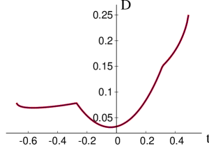
Figure 1: Quantum discord $D=\mathcal{Q}(\rho_{X})$ for $x_{3}=0.1$, $y_{3}=0.2$, $t_{1}=0.2$, $t_{2}=0.3$. Here the results in Li , our numerical results and our upper bound in Eq. (10) agree with high precision.

Now, let us consider the following general two-qubit states, $\rho_{2\times 2}=(I\otimes I+\sum_{i=1}^{3}[x_{i}(\sigma_{i}\otimes I)+y_{i}(I\otimes\sigma_{i})+t_{i}(\sigma_{i}\otimes\sigma_{i})])/4$, and compare our analytical upper bound with numerical results. Fig.2 gives the quantum discord $\mathcal{Q}(\rho_{2\times 2})$, for $x_{1}=0.05$, $x_{2}=0.1$, $x_{3}=0.1$, $y_{1}=0.15$, $y_{2}=0.25$, $y_{3}=0.2$, $t_{1}=0.2$ and $t_{2}=0.2$ plotted against $t_{3}$, such that $\rho_{2\times 2}$ is a quantum state. Fig.3 shows the quantum discord $\mathcal{Q}(\rho_{2\times 2})$ for $x_{2}=0.1$, $x_{3}=0.1$, $y_{1}=0.15$, $y_{2}=0.25$, $y_{3}=0.2$, $t_{1}=0.2$, $t_{2}=0.2$ and $t_{3}=-0.5$, plotted against $x_{1}$, such that $\rho_{2\times 2}$ is a quantum state. It can be seen that our upper bound coincides very well with the numerical results.

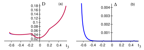
Figure 2: Figure (a) shows quantum discord $D=\mathcal{Q}(\rho_{2\times 2})$. Solid blue line shows numerical results and the red dotted line our upper bound. Figure (b) shows the difference between the numerical results and our upper bound.

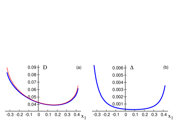
Figure 3: Figure (a) shows quantum discord $D=\mathcal{Q}(\rho_{2\times 2})$. Solid blue line shows numerical results and the red dotted line our upper bound. Figure (b) shows the difference between the numerical results and our upper bound.

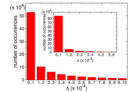
Figure 4: $\Delta$ as a function of number of occurrences for a set of $10^{6}$ random $2\otimes 2$ density matrices.

We have seen that the upper bound of quantum discord based on von Neumann entropy, obtained from the optimal measurements for the classical correlation based on linear entropy, is often exact. To test the precision of our upper bound generally, we calculated the difference between our analytical result and the numerical solution of quantum discord, for a set of $10^{6}$ random density matrices of $2\otimes 2$. In Fig.4, we plot the deviation $\Delta=\mathcal{Q}_{\rm{Analytical}}-\mathcal{Q}_{\rm{Numerical}}$ against the number of occurrences. It can be seen that more than half of the randomly generated density matrices results in a precision greater than $10^{-4}$, which demonstrates that our analytical result is a tight upper bound. Furthermore, in Fig.4, we show that more than $80\%$ of the density matrices randomly generated lead to a precision greater than $10^{-3}$. Indeed, the percentage of density matrices with a deviation $\Delta$ greater than $6\times 10^{-3}$ is less than $0.1\%$. Here, in the horizontal coordinate of Fig. 4, $0..1$ represents the interval from 0 to 1, and the same for $1..2$, etc..

I.3 Evolution of Quantum Discord under AD Channel

Now we consider the evolution of quantum discord for arbitrary $n$-qubit GHZ and W states under an amplitude damping (AD) channel characterized by the Kraus operators $E_{1}=\sqrt{p}\left(\begin{array}[]{cc}0&1\\ 0&0\end{array}\right)$ and $E_{2}=\left(\begin{array}[]{cc}1&0\\ 0&\sqrt{1-p}\end{array}\right)$. We show that the related quantum discord based on von Neumann entropy can be analytically obtained from the upper bound given by Eq. (10).

First let us consider $n$-qubit GHZ states, with the first $(n-1)$ qubits subjected to AD channels individually. From Theorem 2, we get the optimal measurement operators $(I_{2}+\sigma_{z})/2$ and $(I_{2}-\sigma_{z})/2$ for classical correlation in terms of linear entropy, and the upper bound of quantum discord in terms of von Neumann entropy is then exact. Let $M_{1}=U\,P_{0}\,U^{+}$ and $M_{2}=U\,P_{1}\,U^{+}$ be the two measurement operators, where $P_{0}$ and $P_{1}$ are the projective operators, $U=tI_{2}+y_{1}\sigma_{x}+y_{2}\sigma_{y}+y_{3}\sigma_{z}$ with $t^{2}+y_{3}^{2}=\cos^{2}\theta$ and $y_{1}^{2}+y_{2}^{2}=\sin^{2}\theta$. Fig.5 shows that when $\theta=0$ or $\theta=\pi,$ $\sum_{i}p_{i}S(\rho^{A|i})$ has the minimal value, which coincides with the optimal measurement operators $(I_{2}+\sigma_{z})/2$ and $(I_{2}-\sigma_{z})/2$ for classical correlation based on linear entropy.

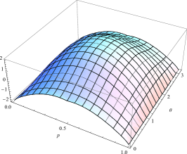
Figure 5: $\sum\limits_{i}p_{i}S(\rho^{A|i})$ as a function of $\theta$ and p.

For $n$-qubit W states with the first $(n-1)$ qubits subjected to individual AD channels, from Theorem 2 we have the optimal measurement operators $(I_{2}+\sigma_{x})/2$ and $(I_{2}-\sigma_{x})/2$ or $(I_{2}+\sigma_{y})/2$ and $(I_{2}-\sigma_{y})/2$. The upper bound of quantum discord obtained in terms of these measurement operators coincide with its lower bound in tightbound . It follows that again we have the exact value of quantum discord (2).

Alternatively, if the last qubit of an $n$-qubit W state is subjected to an AD channel, we have the optimal measurement operators $(I_{2}+\sigma_{x})/2$ and $(I_{2}-\sigma_{x})/2$ or $(I_{2}+\sigma_{y})/2$ and $(I_{2}-\sigma_{y})/2$, which also give rise to the exact value of discord (2).

II Conclusions

We have studied the quantum discord of qudit-qubit states. The analytical formula for classical correlation based on linear entropy has been explicitly derived, from which an analytical tight upper bound of quantum discord based on von Neumann entropy is obtained for arbitrary qudit-qubit states. The upper bound is found to be surprisingly good in the sense that it agrees very well with all known analytical results about quantum discord in terms of von Neumann entropy. Furthermore, for a set of $10^{6}$ random density matrices, the maximum deviation found from the numerical solution was approximately $0.05$ and the number of density matrices whose deviation was greater than $6\times 10^{-3}$ was less than $0.1\%$ of the whole set. Our analytical results could be used to investigate the roles played by quantum discord in quantum information processing. For classical correlation in terms of linear entropy, it has also been shown that the result for a qudit-qubit state, defined by running over all two-operator POVM measurements, is equivalent to that defined by running over all projective measurements. Furthermore, our results can be applied to investigate the evolution of quantum discord for arbitrary $n$-qubit GHZ and W states. Indeed, employing an important paradigmatic noisy channel, we present the quantum discord dynamics for the GHZ and W states when each qubit is subjected to independent amplitude damping channels.

III Acknowledgements

The work is supported by NSFC under numbers 11371247, 10901103 and 11201427. FFF is supported by São Paulo Research Foundation (FAPESP), under grant number 2012/50464-0, and by the National Institute for Science and Technology of Quantum Information (INCT-IQ), under process number 2008/57856-6. FFF is also supported by the National Counsel of Technological and Scientific Development (CNPq) under grant number 474592/2013-8.

IV Author contributions

Z.M. and S.F. prove the main theorems, Z.C. and F.F.F. developed the numerical codes, and Z.M., Z.C., F.F.F. and S.F. wrote the manuscript.

Competing financial interests: The authors declare no competing financial interests.

Appendix A Appendix

[Proof of Theorem 1]   Theorem 1 can be proved by using an approach similar to that used in superdiscord . It was proved by osborne , for the classical correlation $I^{\leftarrow}_{2\,\rm{POVM}}(\rho^{AB})$, of a qudit-qubit state $\rho_{AB}$ defined by running over all POVM measurements(here all POVM means we run over arbitrary POVM, that is, any measurement operators POVM), its optimal POVM measurement must be two operators POVM, that is, we can in fact restrict to two operators POVM. Then let $M(x)$ and $M(-x)$ be two optimal POVM operators, such that $M(x)+M(-x)=I$. Let $\Pi_{0}$ and $\Pi_{1}$ be the projective measurement operators, $\Pi_{0}+\Pi_{1}=I$. We can write the two POVM operators as $M(x)=\sum_{i=0}^{1}a_{i}(x)\Pi_{i}$ and $M(-x)=\sum_{i=0}^{1}a_{i}(-x)\Pi_{i}$, where $a_{0}(x)$ and $a_{1}(x)$ are the eigenvalues of $M(x)$ and $a_{0}(-x)$ and $a_{1}(-x)$ are eigenvalues of $M(-x)$.

Given any qudit-qubit state $\rho_{AB}$, the POVM $\{M(x),M(-x)\}$ performed on subsystem $B$ will yield the post-measurement state $\rho_{A|M^{B}(x)}$. We have $p(x)\rho_{A|M^{B}(x)}=\mbox{Tr}_{B}[\rho_{AB}(I\otimes M(x))]=\sum_{i=0}^{1}a_{i}(x)\,p_{i}\,\rho_{A|\Pi_{i}^{B}}$. From the concavity property of linear entropy, we have the lower bound of the conditional linear entropy,

$$\begin{array}[]{l}\displaystyle\sum_{y=x,-x}p(y)S_{2}(\rho_{A|M^{B}(y)})\\ \displaystyle=\sum_{y=x,-x}p(y)S_{2}(\sum_{i=0}^{1}\frac{a_{i}(y)p_{i}}{p(y)}\rho_{A|\Pi_{i}^{B}})\\ \displaystyle\geq\sum_{y=x,-x}p(y)\sum_{i=0}^{1}\frac{a_{i}(y)p_{i}}{p(y)}S_{2}(\rho_{A|\Pi_{i}^{B}})=\sum_{i=0}^{1}p_{i}S_{2}(\rho_{A|\Pi_{i}^{B}}).\end{array}$$

Thus, the conditional linear entropy derived from POVMs is greater than or equal to the conditional linear entropy derived from the projective measurements, on the all possible measurements basis.

Let $\{{\tilde{\Pi}}_{i}^{B}\}$ be the measurement basis that maximizes the classical correlation $I^{\leftarrow}_{2\,\rm{POVM}}(\rho^{AB})$ for two POVM operators $\{M(x),M(-x)\}$. Then, we have

$$\begin{array}[]{l}\displaystyle I^{\leftarrow}_{2\,\rm{POVM}}(\rho^{AB})=S_{2}(\rho^{A})-\sum_{y=x,-x}p(y)S_{2}(\rho_{A|M^{B}(y)})\\[11.38109pt] ~{}~{}\displaystyle\leq S_{2}(\rho^{A})-\sum_{i}p_{i}S_{2}(\rho_{A|\Pi_{i}^{B}})\displaystyle\leq I^{\leftarrow}_{2\,\rm{PM}}(\rho^{AB}),\end{array}$$

since $\{{\tilde{\Pi}}_{i}^{B}\}$ could be a non-optimal projective measurement of the classical correlation $I^{\leftarrow}_{2\,\rm{PM}}(\rho^{AB})$. Hence, $I^{\leftarrow}_{2\,\rm{POVM}}(\rho^{AB})\leq I^{\leftarrow}_{2\,\rm{PM}}(\rho^{AB})$; i.e., the classical correlation under two POVM measurements is always smaller than or equal to the classical correlation under projective measurements.

On the other hand, a projective measurement is a POVM. Hence, by definition, the classical correlation under two POVM measurements is always greater than or equal to the classical correlation under projective measurement. Therefore, we have proved that the classical correlation under two POVM measurements is equal to the classical correlation under projective measurement, $I^{\leftarrow}_{2\,\rm{POVM}}(\rho^{AB})=I^{\leftarrow}_{2\,\rm{PM}}(\rho^{AB})$. $\hfill\Box$

References

• (1) Nielsen M. A. & Chuang I. L. Quantum Computation and Quantum Information (Cambridge University Press, Cambridge, England, 2000).
• (2) Horodecki R., Horodecki P., Horodecki M., & Horodecki K. Quantum entanglement. Rev. Mod. Phys. 81, 865 (2009).
• (3) GΓΌhne O. & TΓ³th G. Entanglement detection. Phys. Rep. 474, 1 (2009).
• (4) Datta A., Flammia A. T., & Caves C. M. Entanglement and the power of one qubit. Phys. Rev. A 72, 042316 (2005);
• (5) Datta A. & Vidal G. Role of entanglement and correlations in mixed-state quantum computation. Phys. Rev. A 75, 042310 (2007);
• (6) Datta A., Shaji A. & Caves C. M. Quantum discord and the power of one qubit. Phys. Rev. Lett. 100, 050502 (2008);
• (7) Lanyon B. P., Barbieri M., Almeida M. P. & White A. G. Experimental quantum computing without entanglement. Phys. Rev. Lett. 101, 200501 (2008).
• (8) Bennett C. H. et al. Quantum nonlocality without entanglement. Phys. Rev. A 59, 1070 (1999).
• (9) Niset J. & Cerf N. J. Multipartite nonlocality without entanglement in many dimensions. Phys. Rev. A. 74, 052103 (2006).
• (10) Knill E. & Laflamme R. On the power of one bit of quantum information. Phys. Rev. Lett. 81, 5672 (1998).
• (11) Modi K., Brodutch A., Cable H., Paterek T. & Vedral V. The classical-quantum boundary for correlations: discord and related measures. Rev. Mod. Phys. 84, 1655 (2012).
• (12) Ollivier H. & Zurek W. H. Quantum discord: a measure of the quantumness of correlations. Phys. Rev. Lett. 88, 017901 (2001).
• (13) Henderson L. & Vedral V. Classical, quantum and total correlations. J. Phys. A 34, 6899 (2001).
• (14) Roa L., Retamal J. C. & Alid-Vaccarezza M., Dissonance is required for assisted optimal state discrimination. Phys. Rev. Lett. 107, 080401 (2011);
• (15) Li B., Fei S. M., Wang Z. X. & Fan H. Assisted state discrimination without entanglement. Phys. Rev. A 85, 022328 (2012).
• (16) Osborne T. J. & Verstraete F. General monogamy inequality for bipartite qubit entanglement. Phys. Rev. Lett. 96, 220503 (2006).
• (17) Yu S. & Liu N. Entanglement detection by local orthogonal observables. Phys. Rev. Lett. 95, 150504 (2005);
• (18) Hassan A. S. M. & Joag P. S. Separability criterion for multipartite quantum states based on the Bloch representation of density matrices. Quant. Inf. and Comp. 8, 0773 (2008).
• (19) Hughston L. P., Jozsa R. & Wootters W. K. A complete classification of quantum ensembles having a given density matrix. Phys. Lett. A 183, 14 (1993).
• (20) Shi M., Sun C., Jiang F., Yan X. & Du J. Optimal measurement for quantum discord of two-qubit states. Phys. Rev. A 85, 064104 (2012).
• (21) Chen Q., Zhang C., Yu S., Yi X. X. & Oh C. H. Quantum discord of two-qubit X states. Phys. Rev. A 84, 042313 (2011).
• (22) Luo S. Quantum discord for two-qubit systems. Phys. Rev. A 77, 042303 (2008).
• (23) Koashi M. & Winter A. Monogamy of entanglement and other correlations. Phys. Rev. A 69, 022309(2004).
• (24) Li B., Wang Z. & Fei S. Quantum discord and geometry for a class of two-qubit states. Phys. Rev. A 83, 022321 (2011).
• (25) Ali M., Rau A. R. P. & Alber G. Quantum discord for two-qubit X states. Phys. Rev. A 81, 042105 (2010);
• (26) Ali M., Rau A. R. P. & Alber G. Erratum: quantum discord for two-qubit X states. Phys. Rev. A 82, 069902 (2010).
• (27) Vinjanampathy S. & Rau A. R. P. Quantum discord for qubit-qudit systems. J. Phys. A: Math. Theor. 45, 095303 (2012).
• (28) Yu S. X., Zhang C. J., Chen Q. & Oh C.H. Tight bounds for the quantum discord. arXiv: 1102.1301.

References

• (1) Singh U. & Pati A. K. Super quantum discord with weak measurements. Ann. of Phys. 343, 141 (2014).
• (2) Osborne T. J. & Verstraete F. General monogamy inequality for bipartite qubit entanglement. Phys. Rev. Lett. 96, 220503 (2006).