Domain decomposition finite element/finite difference method for the conductivity reconstruction in a hyperbolic equation

Abstract

We present domain decomposition finite element/finite difference method for the solution of hyperbolic equation. The domain decomposition is performed such that finite elements and finite differences are used in different subdomains of the computational domain: finite difference method is used on the structured part of the computational domain and finite elements on the unstructured part of the domain. The main goal of this method is to combine flexibility of finite element method and efficiency of a finite difference method.

An explicit discretization schemes for both methods are constructed such that finite element and finite difference schemes coincide on the common structured overlapping layer between computational subdomains. Then the resulting scheme can be considered as a pure finite element scheme which allows avoid instabilities at the interfaces.

We illustrate efficiency of the domain decomposition method on the reconstruction of the conductivity function in the hyperbolic equation in three dimensions.

1 Introduction

With expanding of new computational technologies and needs of industry it is vital importance to use efficient computational methods for simulation of partial differential equations in two and three-dimensions when computational domains are very large. Domain decomposition methods attracted a lot of interest and is a topic of current research, see, for example, [9, 10] and references therein.

It is typical that computational domains in industrial applications often are very large and only some part of this domain presents interest. In such cases a domain decomposition approach can be attractive when the simple domain discretization can be used in a large region and more complex and refined domain discretization is applied in a smaller part of the domain. In this paper we propose to use domain decomposition finite element/finite difference approach for the solution of hyperbolic equation which combines flexibility of the finite element method (FEM) and efficiency in terms of speed and memory usage of finite difference method (FDM). To do that we extend a hybrid FEM/FDM method which was developed in [5] for the case of acoustic wave equation, to the case of a more general hyperbolic equation with two unknown parameters. Similar to our approach in [5], we decompose the computational domain such that finite elements and finite differences are used in different subdomains of this domain: finite difference method is used in a simple geometry and finite elements - in the subdomain where we want to get more detailed information about structure of this domain. Our goal is to get such a method which will combine flexibility of finite element method and efficiency of a finite difference method. It is well known that the finite element method allows to get small features of the structure of the domain through the adaptive mesh refinement. However, this method is quite computationally expensive comparing with the finite difference method in terms of time and memory usage, see [2]-[6] for study of efficiency of these methods.

In this work we derive explicit schemes for both methods such that finite element and finite difference methods coincide on the common structured overlapping layer between these domains. Thus, the resulting scheme can be considered as a pure finite element scheme which allows to avoid instabilities at the interfaces [8]. We implement this method in an efficient way in the software package WavES [19] in C++ using PETSc [16] and MPI (message passing interface).

We illustrate the efficiency of the proposed method on the solution of the hyperbolic coefficient inverse problem (CIP) in three dimensions. The goal of our numerical simulations is to reconstruct the conductivity function of the hyperbolic equation from single observations of the backscattered solution of this equation in space and time. We note, that the domain decomposition approach in this case is particularly feasible for implementing of absorbing boundary conditions [13]. To solve our CIP we minimize the corresponding Tikhonov functional and use Lagrangian approach to do that. This approach is similar to one applied recently in [2, 3, 6, 7] for the solution of different three-dimensional CIPs: we find optimality conditions which express stationarity of the Lagrangian, involving the solution of a state and adjoint equations together with an equation expressing that the gradient of the Lagrangian with respect to the conductivity vanishes. Then we construct conjugate gradient algorithm and compute the unknown conductivity function in an iterative process by solving in every step of this algorithm the state and adjoint hyperbolic equations and updating in this way the conductivity function.

We tested our inverse algorithm on the reconstruction of conductivity function which represents small symmetrical inclusions. This problem can be interpreted as the problem of the reconstruction of the symmetrical structure of a waveguide and finding defects in it. Our computations show that we can accurately reconstruct large contrast of the conductivity function as well as location of all small inclusions using the domain decomposition method presented in this work.

The paper is organized as follows. In Section 2 we present our mathematical model of hyperbolic equation and in Section 3 we describe domain decomposition approach. Energy estimate for the equation of Section 2 is derived in Section 4. In Section 5 we formulate state and inverse problems for hyperbolic equation. The Tikhonov functional to be minimized and the corresponding Lagrangian are presented in Section 6. In Section 7 we describe the domain decomposition finite element/finite difference method to solve the minimization problem of Section 6. Finally, in Section 9 we demonstrate efficiency of the domain decomposition method on the reconstruction of the conductivity function in three dimensions.

2 The mathematical model

The model problem in the domain decomposition method is the following hyperbolic equation with the first order absorbing boundary conditions [13]

$$\begin{split}\frac{1}{c^{2}}\frac{\partial^{2}u}{\partial t^{2}}-\nabla\cdot(a\nabla u)&=g(x,t),~{}\mbox{in}~{}~{}\Omega_{T},\\ u(x,0)=f_{0}(x),~{}~{}~{}u_{t}(x,0)&=f_{1}(x)~{}\mbox{in}~{}~{}\Omega,\\ \partial_{n}u&=-\partial_{t}u~{}\mbox{on}~{}\partial\Omega_{T},\\ \end{split}$$ (1)

Here $\Omega\subset\mathbb{R}^{3}$ is a convex bounded domain with the boundary $\partial\Omega\in C^{3}$, $x=(x_{1},x_{2},x_{3})\in\mathbb{R}^{3}$ and $C^{k+\alpha}$ is Hölder space, where $k\geq 0$ and $\alpha\in\left(0,\,1\right)$, $c(x),a(x)$ are the wave speed and the conductivity space-dependent functions, respectively. We defined by $\Omega_{T}:=\Omega\times(0,T),\partial\Omega_{T}:=\partial\Omega\times(0,T),T>0$. We assume that

$$g(x,t)\in L_{2}(\Omega_{T}),f_{0}\in H^{1}(\Omega),f_{1}\in L_{2}(\Omega).$$ (2)

For our purpose we use modification of the domain decomposition method developed in [5] which was applied for the solution of the coefficient inverse problem for the acoustic wave equation in [2, 7]. In this work, we use different version of the method used in [2, 5, 7], when two functions - the wave speed $c(x)$ and the conductivity function $a(x)$ - are introduced in the mathematical model of the hyperbolic equation. Similarly with [2]-[7], we decompose $\Omega$ into two open subregions, $\Omega_{FEM}$ and $\Omega_{FDM}$ such that $\Omega=\Omega_{FEM}\cup\Omega_{FDM}$, and $\Omega_{FEM}\cap\Omega_{FDM}=\emptyset$. In $\Omega_{FEM}$ we use finite elements and this domain is such that $\partial\Omega_{FEM}\subset\partial\Omega_{FDM}$, see figure 2. In $\Omega_{FDM}$ we will use finite difference method.

We assume that our coefficients $a(x),c\left(x\right)$ of problem (1) are such that

$$\begin{split}a\left(x\right)&\in\left[1,d_{1}\right],~{}~{}d_{1}=const.>1,~{}a(x)=1\text{ for }x\in\Omega_{FDM},\\ c\left(x\right)&\in\left[1,d_{2}\right],~{}~{}d_{2}=const.>1,~{}c(x)=1\text{ for }x\in\Omega_{FDM},\\ a(x),c(x)&\in C^{2}\left(\mathbb{R}^{3}\right).\end{split}$$ (3)

3 The domain decomposition algorithm

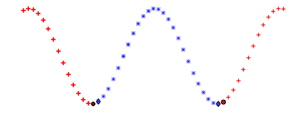
Figure 1: Example of the solution in the domain decomposition between $\Omega_{FEM}$ and $\Omega_{FDM}$ in one dimension with $a=c=1$. The interior nodes of the finite element grid $\Omega_{FEM}$ are denoted by stars, while circles and diamonds denote nodes, which are shared between meshes in $\Omega_{FEM}$ and $\Omega_{FDM}$. The circles are interior nodes of the grid in $\Omega_{FDM}$, while the diamonds are interior nodes of the grid in $\Omega_{FEM}$. At each time iteration, solution obtained in $\Omega_{FDM}$ at $\omega_{\rm o}$ is copied to the corresponding boundary nodes in $\Omega_{FEM}$, while simultaneously the solution obtained in $\Omega_{FEM}$ at $\omega_{\diamond}$ is copied to the corresponding boundary nodes in $\Omega_{FDM}$.

We now describe the domain decomposition between $\Omega_{FEM}$ and $\Omega_{FDM}$ domains. This communication is achieved by mesh overlapping across a two-element thick layer around $\Omega_{FEM}$ - see Figure  1. First, using the Figure 1 we observe that the interior nodes of the computational domain $\Omega$ belong to either of the following sets:

• Nodes ’$\rm o$’ - lie on the boundary of $\Omega_{FEM}$ and are interior to $\Omega_{FDM}$,

• Nodes ’$\diamond$’ - lie on the boundary of $\Omega_{FDM}$ and are interior to $\Omega_{FEM}$,

• Nodes ’$*$’ are interior to $\Omega_{FEM}$,

• Nodes ’$+$’ are interior to $\Omega_{FDM}$

Then the main loop in time for the explicit schemes which solves the problem (1) is as follows:

Algorithm 1

At every time step $k$ we perform the following operations:

1. On the structured part of the mesh $\Omega_{FDM}$ update the FDM solution at nodes $\omega_{+}$ and $\omega_{\diamond}$.

2. On the unstructured part of the mesh $\Omega_{FEM}$ update the FEM solution at nodes $\omega_{*}$ and $\omega_{\rm o}$.

3. Copy FEM solution obtained at nodes $\omega_{\diamond}$ as a boundary condition for the FDM solution in $\Omega_{FDM}$.

4. Copy FDM solution obtained at nodes $\omega_{\rm o}$ as a boundary condition for the FEM solution in $\Omega_{FEM}$.

4 Energy estimate

In this section we prove the uniqueness theorem, or energy estimate, for the function $u\in H^{2}\left(\Omega_{T}\right)$ of the problem (1), using the technique of [15].

Theorem

Assume that condition (3) on the functions $c(x),a(x)$ hold. Let $\Omega\subset\mathbb{R}^{3}$ be a bounded domain with the piecewise smooth boundary $\partial\Omega$.  For any $t\in\left(0,T\right)$ let $\Omega_{t}=\Omega\times\left(0,t\right).$  Suppose that there exists a solution $u\in H^{2}(\Omega_{T})$ of the problem (1). Then the function $u$ is unique and there exists a constant $A=A(||c||_{\Omega},||a||_{\Omega},t)$  such that the following energy estimate is true for all $c,a\geq 1$ in (1)

$$\begin{split}\left\|\sqrt{\frac{1}{c^{2}}}\partial_{t}u(x,t)\right\|_{L_{2}\left(\Omega\right)}^{2}+\left\|\sqrt{a}\nabla u(x,t)\right\|_{L_{2}\left(\Omega\right)}^{2}\leq A\left[\left\|g\right\|_{L_{2}\left(\Omega_{t}\right)}^{2}+\left\|\sqrt{\frac{1}{c^{2}}}f_{1}\right\|_{L_{2}\left(\Omega\right)}^{2}+\left\|\sqrt{a}\nabla f_{0}\right\|_{L_{2}\left(\Omega\right)}^{2}\right].\end{split}$$ (4)

Proof.

First we multiply hyperbolic equation in (1) by $2\partial_{t}u$ and integrate over $\Omega\times\left(0,t\right)$ to get

$$\begin{split}\int\limits_{0}^{t}\int\limits_{\Omega}2~{}\frac{1}{c^{2}}\partial_{tt}u~{}\partial_{t}u~{}dxd\tau-\int\limits_{0}^{t}\int\limits_{\Omega}2\nabla\cdot(a\nabla u)~{}\partial_{t}u~{}dxd\tau=2\int\limits_{0}^{t}\int\limits_{\Omega}g~{}\partial_{t}u~{}dxd\tau.\end{split}$$ (5)

Integrating in time the first term of (5) we get

$$\int\limits_{0}^{t}\int\limits_{\Omega}\partial_{t}(\frac{1}{c^{2}}\partial_{t}u^{2})dxd\tau=\int\limits_{\Omega}\left(\frac{1}{c^{2}}\partial_{t}u^{2}\right)\left(x,t\right)dx-\int\limits_{\Omega}\frac{1}{c^{2}}f_{1}^{2}\left(x,t\right)dx.$$ (6)

Integrating by parts in space the second term of (5), using conditions (3) giving $a=1$ on $\partial\Omega$, and absorbing boundary conditions in (1) we get

$$\begin{split}&2\int\limits_{0}^{t}\int\limits_{\Omega}\nabla\cdot\left(a\nabla u\right)\partial_{t}udxd\tau\\ &=2\int\limits_{0}^{t}\int\limits_{\partial\Omega}\left(\partial_{t}u\right)\partial_{n}udSd\tau-2\int\limits_{0}^{t}\int\limits_{\Omega}\left(a\nabla u\right)\left(\nabla\partial_{t}u\right)dxd\tau\\ &=-\int\limits_{0}^{t}\int\limits_{\partial\Omega}\left(\partial_{t}u\right)^{2}~{}dSd\tau-\int\limits_{0}^{t}\int\limits_{\Omega}a\partial_{t}|\nabla u|^{2}dxd\tau.\end{split}$$ (7)

Integrating last term of (7) in time and using initial conditions of the equation (1) we obtain

$$\begin{split}&-\int\limits_{0}^{t}\int\limits_{\Omega}a\partial_{t}|\nabla u|^{2}dxd\tau=-\int\limits_{\Omega}a|\nabla u|^{2}\left(x,t\right)dx+\int\limits_{\Omega}a|\nabla u|^{2}\left(x,0\right)dx\\ &=-\int\limits_{\Omega}a|\nabla u|^{2}\left(x,t\right)dx+\int\limits_{\Omega}a|\nabla f_{0}|^{2}\left(x\right)dx.\end{split}$$ (8)

Next, collecting estimates (6), (7), (8), using the fact that $\int\limits_{0}^{t}\int\limits_{\partial\Omega}\left(\partial_{t}u\right)^{2}~{}dSd\tau\geq 0$ and substituting them in (5) we have

$$\begin{split}&\int\limits_{\Omega}\left(\frac{1}{c^{2}}\partial_{t}u^{2}\right)\left(x,t\right)dx+\int\limits_{\Omega}a|\nabla u|^{2}\left(x,t\right)dx\\ &\leq 2\int\limits_{0}^{t}\int\limits_{\Omega}|g|~{}|\partial_{t}u|~{}dxd\tau+\int\limits_{\Omega}\frac{1}{c^{2}}f_{1}^{2}\left(x,t\right)dx+\int\limits_{\Omega}a|\nabla f_{0}|^{2}\left(x\right)dx.\end{split}$$ (9)

Finally, to estimate the first term in the right hand side of (9) we use the arithmetic-geometric mean inequality $2ab\leq a^{2}+b^{2}$ to obtain

$$2\int\limits_{0}^{t}\int\limits_{\Omega}|g|\cdot|\partial_{t}u|~{}dxd\tau\leq\int\limits_{0}^{t}\int\limits_{\Omega}|g|^{2}dxd\tau+\int\limits_{0}^{t}\int\limits_{\Omega}|\partial_{t}u|^{2}dxd\tau.$$ (10)

Noting that using (3) we can write following estimate

$$\int\limits_{0}^{t}\int\limits_{\Omega}|\partial_{t}u|^{2}~{}dxd\tau\leq\int\limits_{0}^{t}\int\limits_{\Omega}\left(\frac{1}{c^{2}}|\partial_{t}u|^{2}+a|\nabla u|^{2}\right)~{}dxd\tau,$$

and substituting the above estimate into (10) and then the resulting estimate into (9) we have the following estimate

$$\begin{split}\int\limits_{\Omega}\left(\frac{1}{c^{2}}\partial_{t}u^{2}+a\left|\nabla u\right|^{2}\right)(x,t)dx&\leq\int\limits_{0}^{t}\int\limits_{\Omega}|g|^{2}dxd\tau+\int\limits_{0}^{t}\int\limits_{\Omega}\left(\frac{1}{c^{2}}|\partial_{t}u|^{2}+a|\nabla u|^{2}\right)~{}dxd\tau\\ &+\int\limits_{\Omega}\left(\frac{1}{c^{2}}f_{1}^{2}+a\left|\nabla f_{0}\right|^{2}\right)(x,t)dx.\end{split}$$ (11)

Let us denote

$$F(t):=\int\limits_{\Omega}\left(\frac{1}{c^{2}}\partial_{t}u^{2}+a\left|\nabla u\right|^{2}\right)\left(x,t\right)dx.$$ (12)

We rewrite estimate (11) in the form

$$F(t)\leq A\int_{0}^{t}F(\tau)d\tau+r(t),$$ (13)

where $r(t):=\int\limits_{0}^{t}\int\limits_{\Omega}|g|^{2}dxd\tau+\int\limits_{\Omega}\left(\frac{1}{c^{2}}f_{1}^{2}+a\left|\nabla f_{0}\right|^{2}\right)\left(x,t\right)dx.$

Applying Grönwall’s inequality to (13) with a constant $A=A(||c||_{\Omega},||a||_{\Omega},t)$ we get desired energy estimate (4) which also can be written in the form

$$\begin{split}\int\limits_{\Omega}\left(\frac{1}{c^{2}}\partial_{t}u^{2}+a\left|\nabla u\right|^{2}\right)(x,t)dx\leq A\left(\int\limits_{0}^{t}\int\limits_{\Omega}|g|^{2}dxd\tau+\int\limits_{\Omega}\left(\frac{1}{c^{2}}f_{1}^{2}+a\left|\nabla f_{0}\right|^{2}\right)\left(x,t\right)dx\right).\end{split}$$ (14)

$\square$

5 Statement of the forward and inverse problems

In this section we state the forward and inverse problems. In section 8 we will show how these problems can be solved using the domain decomposition algorithm of section 3.

Let the boundary $\partial\Omega$ is such that $\partial\Omega=\partial_{1}\Omega\cup\partial_{2}\Omega\cup\partial_{3}\Omega$ where $\partial_{1}\Omega$ and $\partial_{2}\Omega$ are, respectively, front and back sides of the domain $\Omega$, and $\partial_{3}\Omega$ is the union of left, right, top and bottom sides of this domain. Let at $S_{T}:=\partial_{1}\Omega\times(0,T)$ we will have time-dependent observations at the backscattering side $\partial_{1}\Omega$ of the domain $\Omega$. We also define $S_{1,1}:=\partial_{1}\Omega\times(0,t_{1}]$, $S_{1,2}:=\partial_{1}\Omega\times(t_{1},T)$, $S_{2}:=\partial_{2}\Omega\times(0,T)$ and $S_{3}:=\partial_{3}\Omega\times(0,T)$.

We have used 2 model problems in our computations.

Model Problem 1

The first model problem is the same as (1) but when $c(x)=1~{}~{}\forall x\in\Omega$ and with non-homogeneous initial conditions:

$$\begin{split}\frac{\partial^{2}u}{\partial t^{2}}-\nabla\cdot(a\nabla u)&=0,~{}\mbox{in}~{}~{}\Omega_{T},\\ u(x,0)=f_{0}(x),~{}~{}~{}u_{t}(x,0)&=f_{1}(x)~{}\mbox{in}~{}~{}\Omega,\\ \partial_{n}u&=p\left(t\right)~{}\mbox{on}~{}S_{1,1},\\ \partial_{n}u&=-\partial_{t}u~{}\mbox{on}~{}S_{1,2},\\ \partial_{n}u&=-\partial_{t}u~{}\mbox{on}~{}S_{2},\\ \partial_{n}u&=0~{}\mbox{on}~{}S_{3}.\\ \end{split}$$ (15)

Model Problem 2

Our model problem 2 uses homogeneous initial conditions and $c(x)=1~{}~{}\forall x\in\Omega$ in (1) and is defined as

$$\begin{split}\frac{\partial^{2}u}{\partial t^{2}}-\nabla\cdot(a\nabla u)&=0,~{}\mbox{in}~{}~{}\Omega_{T},\\ u(x,0)=0,~{}~{}~{}u_{t}(x,0)&=0~{}\mbox{in}~{}~{}\Omega,\\ \partial_{n}u&=p\left(t\right)~{}\mbox{on}~{}S_{1,1},\\ \partial_{n}u&=-\partial_{t}u~{}\mbox{on}~{}S_{1,2},\\ \partial_{n}u&=-\partial_{t}u~{}\mbox{on}~{}S_{2},\\ \partial_{n}u&=0~{}\mbox{on}~{}S_{3}.\\ \end{split}$$ (16)

We assume that our coefficient $a\left(x\right)$ of problems (15) and (16) is such that

$$\begin{split}a\left(x\right)&\in\left[1,d\right],~{}~{}d=const.>1,~{}a(x)=1\text{ for }x\in\Omega_{FDM},\\ a\left(x\right)&\in C^{2}\left(\mathbb{R}^{3}\right).\end{split}$$ (17)

We consider the following

Inverse Problem 1 (IP1) Suppose that the coefficient $a\left(x\right)$  in the problem (15) satisfies (17). Assume that the function $a\left(x\right)$ is unknown in the domain $\Omega\diagdown\Omega_{FDM}$. Determine the function $a\left(x\right)$  in (15) for $x\in\Omega\diagdown\Omega_{FDM},$  assuming that the following function $\tilde{u}\left(x,t\right)$ is known

$$u\left(x,t\right)=\tilde{u}\left(x,t\right),\forall\left(x,t\right)\in S_{T}.$$ (18)

The question of stability and uniqueness of IP1 is addressed in the recent work [12].

Inverse Problem 2 (IP2) Suppose that the coefficient $a\left(x\right)$  in the problem (16) satisfies (17). Assume that the function $a\left(x\right)$ is unknown in the domain $\Omega\diagdown\Omega_{FDM}$. Determine the function $a\left(x\right)$  in (16) for $x\in\Omega\diagdown\Omega_{FDM},$  assuming that the following function $\tilde{u}\left(x,t\right)$ is known

$$u\left(x,t\right)=\tilde{u}\left(x,t\right),\forall\left(x,t\right)\in S_{T}.$$ (19)

6 Optimization method

In this section we will reformulate our inverse problem IP1 as an optimization problem to be able to reconstruct the unknown function $a(x)$ in (15) with best fit to time and space domain observations $\tilde{u}$, measured at a finite number of observation points on $\partial_{1}\Omega$. Solution of IP2 follows from the solution of IP1 by taking $f_{0}=f_{1}=0$.

Our goal is to minimize the Tikhonov functional

$$F(u,a)=\frac{1}{2}\int_{S_{T}}(u-\tilde{u})^{2}z_{\delta}(t)dxdt+\frac{1}{2}\gamma\int_{\Omega}(a-a_{0})^{2}~{}~{}dx,$$ (20)

where $\tilde{u}$ is the observed field, $u$ satisfies the equations (15), and thus depends on $a$, $a_{0}$ is the initial guess for $a$, and $\gamma$ is the regularization parameter. Here, $z_{\delta}(t)$ is a cut-off function, which is introduced to ensure that the compatibility conditions at $\overline{\Omega}_{T}\cap\left\{t=T\right\}$ for the adjoint problem (27). The function $z_{\delta}$ can be chosen similarly with [3].

For our theoretical investigations we introduce the following spaces of real valued functions

$$\begin{split}H_{u}^{1}&:=\{w\in H^{1}(\Omega_{T}):w(\cdot,0)=0\},\\ H_{\lambda}^{1}&:=\{w\in H^{1}(\Omega_{T}):w(\cdot,T)=0\},\\ U^{1}&=H_{u}^{1}(\Omega_{T})\times H_{\lambda}^{1}(\Omega_{T})\times C\left(\overline{\Omega}\right),\\ U^{0}&=L_{2}\left(\Omega_{T}\right)\times L_{2}\left(\Omega_{T}\right)\times L_{2}\left(\Omega\right).\end{split}$$ (21)

To solve this minimization problem for model problem (15) we introduce the Lagrangian

$$\begin{split}L(v)&=F(u,a)-\int_{\Omega_{T}}\frac{\partial\lambda}{\partial t}\frac{\partial u}{\partial t}~{}dxdt+\int_{\Omega_{T}}(a\nabla u)(\nabla\lambda)~{}dxdt\\ &-\int_{\Omega}\lambda(x,0)f_{1}(x)~{}dx-\int_{S_{1,1}}\lambda p(t)~{}d\sigma dt+\int_{S_{1,2}}\lambda\partial_{t}u~{}d\sigma dt+\int_{S_{2}}\lambda\partial_{t}u~{}d\sigma dt,\\ \end{split}$$ (22)

where $v=(u,\lambda,a)\in U^{1}$, and search for a stationary point with respect to $v$ satisfying $\forall\bar{v}=(\bar{u},\bar{\lambda},\bar{a})\in U^{1}$

$$L^{\prime}(v;\bar{v})=0,$$ (23)

where $L^{\prime}(v;\cdot)$ is the Jacobian of $L$ at $v$.

As usual, we assume that $\lambda\left(x,T\right)=\partial_{t}\lambda\left(x,T\right)=0$ and impose such conditions on the function $\lambda$ that $L\left(u,\lambda,a\right):=L\left(v\right)=F\left(u,a\right).$ We also use the facts that $\lambda(x,T)=\frac{\partial\lambda}{\partial t}(x,T)=0$ as well as $a=1$ on $\partial\Omega$, together with initial conditions of (15) and boundary conditions $\partial_{n}u=0$ on $S_{3}$ and $\partial_{n}\lambda=0$ on $\Omega_{T}\setminus S_{T}$. The equation (23) expresses that for all $\bar{v}\in U^{1}$,

$$\begin{split}0=\frac{\partial L}{\partial\lambda}(u)(\bar{\lambda})=&-\int_{\Omega_{T}}\frac{\partial\bar{\lambda}}{\partial t}\frac{\partial u}{\partial t}~{}dxdt+\int_{\Omega_{T}}(a\nabla u)(\nabla\bar{\lambda})~{}dxdt-\int_{\Omega}\bar{\lambda}(x,0)f_{1}(x)~{}dx\\ &-\int_{S_{1,1}}\bar{\lambda}p(t)~{}d\sigma dt+\int_{S_{1,2}}\bar{\lambda}\partial_{t}u~{}d\sigma dt+\int_{S_{2}}\bar{\lambda}\partial_{t}u~{}d\sigma dt,~{}~{}\forall\bar{\lambda}\in H_{\lambda}^{1}(\Omega_{T}),\\ \end{split}$$ (24)

$$\begin{split}0=\frac{\partial L}{\partial u}(u)(\bar{u})&=\int_{S_{T}}(u-\tilde{u})~{}\bar{u}~{}z_{\delta}~{}dxdt-\int_{\Omega}\frac{\partial{\lambda}}{\partial t}(0)\bar{u}(x,0)~{}dx\\ &-\int_{\Omega_{T}}\frac{\partial\lambda}{\partial t}\frac{\partial\bar{u}}{\partial t}~{}dxdt+\int_{\Omega_{T}}(a\nabla\lambda)(\nabla\bar{u})~{}dxdt~{}~{}\forall\bar{u}\in H_{u}^{1}(\Omega_{T}).\\ \end{split}$$ (25)

Finally, we obtain the equation which expresses that the gradient with respect to $a$ vanish:

$$0=\frac{\partial L}{\partial a}(u)(\bar{a})=\int_{\Omega_{T}}(\nabla u)(\nabla\lambda)\bar{a}~{}dxdt+\gamma\int_{\Omega}(a-a_{0})\bar{a}~{}dx,~{}x\in\Omega.$$ (26)

The equation (24) is the weak formulation of the state equation (15) and the equation (25) is the weak formulation of the following adjoint problem

$$\begin{split}\frac{\partial^{2}\lambda}{\partial t^{2}}-\nabla\cdot(a\nabla\lambda)&=-(u-\tilde{u})z_{\delta},~{}x\in S_{T},\\ \lambda(\cdot,T)&=\frac{\partial\lambda}{\partial t}(\cdot,T)=0,\\ \partial_{n}\lambda&=0,~{}\mbox{on}~{}\Omega_{T}\setminus S_{T}.\end{split}$$ (27)

We note that the Lagrangian (22) and the optimality conditions (24), (25) for the model problem 2 will be the same, as for the model problem 1, and only the difference will be that these expressions will note have terms with initial conditions.

7 The domain decomposition FEM/FDM method

In this section we formulate finite element and finite difference methods for the solution of model problem 2. FEM for model problem 1 is the same only terms with non-zero initial conditions should be induced in the discretization.

7.1 Finite element discretization

We discretize $\Omega_{{FEM}_{T}}=\Omega_{FEM}\times(0,T)$ denoting by $K_{h}=\{K\}$ a partition of the domain $\Omega_{FEM}$ into tetrahedra $K$ ($h=h(x)$ being a mesh function, defined as $h|_{K}=h_{K}$, representing the local diameter of the elements), and we let $J_{\tau}$ be a partition of the time interval $(0,T)$ into time intervals $J=(t_{k-1},t_{k}]$ of uniform length $\tau=t_{k}-t_{k-1}$. We assume also a minimal angle condition on the $K_{h}$ [8].

To formulate the finite element method, we define the finite element spaces $C_{h}$, $W_{h}^{u}$ and $W_{h}^{\lambda}$. First we introduce the finite element trial space $W_{h}^{u}$ for $u$ defined by

$$W_{h}^{u}:=\{w\in H_{u}^{1}:w|_{K\times J}\in P_{1}(K)\times P_{1}(J),\forall K\in K_{h},\forall J\in J_{\tau}\},$$

where $P_{1}(K)$ and $P_{1}(J)$ denote the set of linear functions on $K$ and $J$, respectively. We also introduce the finite element test space $W_{h}^{\lambda}$ defined by

$$W_{h}^{\lambda}:=\{w\in H_{\lambda}^{1}:w|_{K\times J}\in P_{1}(K)\times P_{1}(J),\forall K\in K_{h},\forall J\in J_{\tau}\}.$$

To approximate function $a(x)$ we will use the space of piecewise constant functions $C_{h}\subset L_{2}(\Omega)$,

$$C_{h}:=\{u\in L_{2}(\Omega):u|_{K}\in P_{0}(K),\forall K\in K_{h}\},$$ (28)

where $P_{0}(K)$ is the piecewise constant function on $K$.

Next, we define $V_{h}=W_{h}^{u}\times W_{h}^{\lambda}\times C_{h}$. The finite element method now reads: Find $v_{h}\in V_{h}$, such that

$$L^{\prime}(v_{h})(\bar{v})=0~{}\forall\bar{v}\in V_{h}.$$ (29)

The equation (29) expresses that the finite element method for the forward problem (16) in $\Omega_{FEM}$ will be: Find $u_{h}\in W_{h}^{u}$, such that $\forall\bar{\lambda}\in W_{h}^{\lambda}$ and for known $a_{h}\in C_{h}$,

$$\begin{split}&-\int_{\Omega_{FEM_{T}}}\frac{\partial\bar{\lambda}}{\partial t}\frac{\partial u_{h}}{\partial t}~{}dxdt-\int_{\partial\Omega_{FEM}}\partial_{n}u_{h}\bar{\lambda}~{}dxdt+\int_{\Omega_{FEM_{T}}}(a_{h}\nabla u_{h})(\nabla\bar{\lambda})~{}dxdt=0,\end{split}$$ (30)

and the finite element method for the adjoint problem (27) in $\Omega_{FEM}$ reads: Find $\lambda_{h}\in W_{h}^{\lambda}$, such that $\forall\bar{u}\in W_{h}^{u}$ and for known $a_{h}\in C_{h}$,

$$\begin{split}&-\int_{\Omega_{FEM}}\frac{\partial{\lambda_{h}}}{\partial t}(0)\bar{u}(x,0)~{}dx-\int_{\Omega_{FEM_{T}}}\frac{\partial\lambda_{h}}{\partial t}\frac{\partial\bar{u}}{\partial t}~{}dxdt\\ &-\int_{\partial\Omega_{FEM}}\partial_{n}\lambda_{h}\bar{u}~{}dxdt+\int_{\Omega_{FEM_{T}}}(a_{h}\nabla\lambda_{h})(\nabla\bar{u})~{}dxdt=0.\end{split}$$ (31)

We note that usually $\dim V_{h}<\infty$ and $V_{h}\subset U^{1}$ as a set and we consider $V_{h}$ as a discrete analogue of the space $U^{1}.$ We introduce the same norm in $V_{h}$ as the one in $U^{0}$,

$$\left\|\bullet\right\|_{V_{h}}:=\left\|\bullet\right\|_{U^{0}},$$ (32)

where $U_{0}$ is defined in (21). From (32) follows that in finite dimensional spaces all norms are equivalent. This allows us in numerical simulations compute coefficients in the space $C_{h}$. However, in the finite element discretization we write $a\in L_{2}(\Omega)$ to allow the function $a(x)$ be approximated in any other finite element space.

7.2 Fully discrete scheme in $\Omega_{FEM}$

In this section we present explicit schemes for computations of the solutions of forward and adjoint problems in $\Omega_{FEM}$. After expanding functions $u_{h}(x,t)$ and $\lambda_{h}(x,t)$ in terms of the standard continuous piecewise linear functions $\{\varphi_{i}(x)\}_{i=1}^{M}$ in space and $\{\psi_{k}(t)\}_{k=1}^{N}$ in time as

$$\begin{split}u_{h}(x,t)&=\sum_{k=1}^{N}\sum_{i=1}^{M}u_{h_{i,k}}\varphi_{i}(x)\psi_{k}(t),\\ \lambda_{h}(x,t)&=\sum_{k=1}^{N}\sum_{i=1}^{M}\lambda_{h_{i,k}}\varphi_{i}(x)\psi_{k}(t),\end{split}$$

where $u_{h_{i,k}}$ and $\lambda_{h_{i,k}}$ denote unknown coefficients at the mesh point $x_{i}\in K_{h}$ and time moment $t_{k}\in J_{\tau}$, substitute them into (30) and (31), correspondingly, with $\bar{\lambda}(x,t)=\bar{u}(x,t)=\sum_{l=1}^{N}\sum_{j=1}^{M}\varphi_{j}(x)\psi_{l}(t)$. We note that we use finite element method only inside $\Omega_{FEM}$, and thus we will have discrete solutions $u_{h_{FDM}}:=u_{{h_{FDM}}_{i,k}}$ and $\lambda_{h_{FDM}}:=\lambda_{{h_{FDM}}_{i,k}}$ obtained in $\Omega_{FDM}$ as the boundary conditions at $\partial\Omega_{FEM}$, after exchange procedure. We obtain the system of discrete equations:

$$\begin{split}&-\sum_{K\in\Omega_{FEM}}\sum_{k,l=1}^{N}\sum_{i,j=1}^{M}u_{h_{i,k}}\int_{K}\varphi_{i}(x)\varphi_{j}(x)\int_{t_{k-1}}^{t_{k+1}}\partial_{t}\psi_{k}(t)\partial_{t}\psi_{l}(t)~{}dxdt\\ &-\sum_{\partial K\in\partial\Omega_{FEM}}\sum_{k,l=1}^{N}\sum_{i,j=1}^{M}u_{h_{i,k}}\int_{\partial K}\partial_{n}\varphi_{i}(x)\varphi_{j}(x)\int_{t_{k-1}}^{t_{k+1}}\psi_{k}(t)\psi_{l}(t)~{}dSdt\\ &+\sum_{K\in\Omega_{FEM}}\sum_{k,l=1}^{N}\sum_{i,j=1}^{M}u_{h_{i,k}}\int_{K}a_{h}\nabla\varphi_{i}(x)\nabla\varphi_{j}(x)\int_{t_{k-1}}^{t_{k+1}}\psi_{k}(t)\psi_{l}(t)~{}dxdt=0.\end{split}$$ (33)

For the case of adjoint problem (27) we get the system of discrete equations:

$$\begin{split}&-\sum_{K\in\Omega_{FEM}}\sum_{k,l=1}^{N}\sum_{i,j=1}^{M}\lambda_{h_{i,k}}\int_{K}\varphi_{i}(x)\varphi_{j}(x)\int_{t_{k-1}}^{t_{k+1}}\partial_{t}\psi_{k}(t)\partial_{t}\psi_{l}(t)~{}dxdt\\ &-\sum_{\partial K\in\partial\Omega_{FEM}}\sum_{k,l=1}^{N}\sum_{i,j=1}^{M}\lambda_{h_{i,k}}\int_{\partial K}\partial_{n}\varphi_{i}(x)\varphi_{j}(x)\int_{t_{k-1}}^{t_{k+1}}\psi_{k}(t)\psi_{l}(t)~{}dSdt\\ &+\sum_{K\in\Omega_{FEM}}\sum_{k,l=1}^{N}\sum_{i,j=1}^{M}\lambda_{h_{i,k}}\int_{K}a_{h}\nabla\varphi_{i}(x)\nabla\varphi_{j}(x)\int_{t_{k-1}}^{t_{k+1}}\psi_{k}(t)\psi_{l}(t)~{}dxdt=0.\\ \end{split}$$ (34)

Next, we compute explicitly time integrals in (33) and (34) using the standard definition of piecewise-linear functions in time, see [4] for details of this computation, and get the following systems of linear equations:

$$\begin{split}M(\mathbf{u}^{k+1}-2\mathbf{u}^{k}+\mathbf{u}^{k-1})&=-\tau^{2}G(\frac{1}{6}\mathbf{u}^{k-1}+\frac{2}{3}\mathbf{u}^{k}+\frac{1}{6}\mathbf{u}^{k+1})-\tau^{2}K(\frac{1}{6}\mathbf{u}^{k-1}+\frac{2}{3}\mathbf{u}^{k}+\frac{1}{6}\mathbf{u}^{k+1}),\\ M(\boldsymbol{\lambda}^{k+1}-2\boldsymbol{\lambda}^{k}+\boldsymbol{\lambda}^{k-1})&=-\tau^{2}G(\frac{1}{6}\boldsymbol{\lambda}^{k-1}+\frac{2}{3}\boldsymbol{\lambda}^{k}+\frac{1}{6}\boldsymbol{\lambda}^{k+1})-\tau^{2}K(\frac{1}{6}\boldsymbol{\lambda}^{k-1}+\frac{2}{3}\boldsymbol{\lambda}^{k}+\frac{1}{6}\boldsymbol{\lambda}^{k+1}),\\ \end{split}$$ (35)

with initial conditions :

$$u(\cdot,0) =\frac{\partial u}{\partial t}(\cdot,0)=0,$$ (36)

$$\lambda(\cdot,T) =\frac{\partial\lambda}{\partial t}(\cdot,T)=0.$$ (37)

Here, $M$ is the block mass matrix in space, $K$ is the block stiffness matrix, $G$ is the block matrix in space at $\partial\Omega_{FEM}$, $S^{k}$ is the load vector at time level $t_{k}$, $\mathbf{u}^{k}$ and $\boldsymbol{\lambda}^{k}$ denote the nodal values of $u_{h}(\cdot,t_{k})$ and $\lambda_{h}(\cdot,t_{k})$, respectively, $\tau$ is the time step.

Now we define the mapping $F_{K}$ for the reference element $\hat{K}$ such that $F_{K}(\hat{K})=K$ and let $\hat{\varphi}$ be the piecewise linear local basis function on the reference element $\hat{K}$ such that $\varphi\circ F_{K}=\hat{\varphi}$. Then the explicit formulas for the entries in system (35) at each element $K$ can be given as:

$$\begin{split}M_{i,j}^{K}&=(~{}\varphi_{i}\circ F_{K},\varphi_{j}\circ F_{K})_{K},\\ K_{i,j}^{K}&=(a_{h}\nabla\varphi_{i}\circ F_{K},\nabla\varphi_{j}\circ F_{K})_{K},\\ G_{i,j}^{\partial K}&=(\partial_{n}\varphi_{i}\circ F_{K},\varphi_{j}\circ F_{K})_{\partial K},\\ \end{split}$$ (38)

where $(\cdot,\cdot)_{K}$ denotes the $L_{2}(K)$ scalar product and $\partial K$ is the part of the boundary of element $K$ which lies at $\partial\Omega_{FEM}$.

To obtain an explicit scheme we approximate $M$ with the lumped mass matrix $M^{L}$, see [11] for details about mass lumping procedure. We also approximate terms corresponding to the mass matrix in time, $\frac{1}{6}\mathbf{u}^{k-1}+\frac{2}{3}\mathbf{u}^{k}+\frac{1}{6}\mathbf{u}^{k+1}$ and $\frac{1}{6}\boldsymbol{\lambda}^{k-1}+\frac{2}{3}\boldsymbol{\lambda}^{k}+\frac{1}{6}\boldsymbol{\lambda}^{k+1}$, by $\mathbf{u}^{k}$ and $\boldsymbol{\lambda}^{k}$, respectively, which fits to the procedure of mass lumping in time. Next, we multiply (35) with $(M^{L})^{-1}$ and get the following explicit method:

$$\begin{split}\mathbf{u}^{k+1}=&(2-\tau^{2}(M^{L})^{-1}K)\mathbf{u}^{k}-\tau^{2}(M^{L})^{-1}G\mathbf{u}^{k}-\mathbf{u}^{k-1},\\ \boldsymbol{\lambda}^{k-1}=&-\tau^{2}(M^{L})^{-1}G\boldsymbol{\lambda}^{k}+(2-\tau^{2}(M^{L})^{-1}K)\boldsymbol{\lambda}^{k}-\boldsymbol{\lambda}^{k+1}.\\ \end{split}$$ (39)

Finally, for reconstructing $a(x)$ in $\Omega_{FEM}$ we can use a gradient-based method with an appropriate initial guess values of $a_{0}$. The discrete version in space of the gradient with respect to coefficient $a$ in (26) take the form:

$$g_{h}(x)=\int_{0}^{T}\nabla u_{h}\nabla\lambda_{h}dt+\gamma(a_{h}-a_{0}).$$ (40)

Here, $\lambda_{h}$ and $u_{h}$ are computed values of the adjoint and forward problems using explicit schemes (39), and $a_{h}$ are approximated values of the computed coefficient.

7.3 Finite difference formulation

We recall now that from conditions (17) it follows that in $\Omega_{FDM}$ the function $a(x)=1$. This means that in $\Omega_{FDM}$ for the model problem (15) the forward problem will be

$$\begin{split}\frac{\partial^{2}u}{\partial t^{2}}-\Delta u&=0,~{}\mbox{in}~{}~{}\Omega_{T},\\ u(x,0)=f_{0}(x),~{}~{}~{}u_{t}(x,0)&=f_{1}(x)~{}\mbox{in}~{}~{}\Omega_{FDM},\\ \partial_{n}u&=p\left(t\right)~{}\mbox{on}~{}S_{1,1},\\ \partial_{n}u&=-\partial_{t}u~{}\mbox{on}~{}S_{1,2},\\ \partial_{n}u&=-\partial_{t}u~{}\mbox{on}~{}S_{2},\\ \partial_{n}u&=0~{}\mbox{on}~{}S_{3},\\ \partial_{n}u&=\partial_{n}u_{FEM}~{}\mbox{on}~{}\partial\Omega_{FEM}.\\ \end{split}$$ (41)

Then the corresponding adjoint problem in $\Omega_{FDM}$ will be:

$$\begin{split}\frac{\partial^{2}\lambda}{\partial t^{2}}-\Delta\lambda&=-(u-\tilde{u})z_{\delta},~{}x\in S_{T},\\ \lambda(\cdot,T)&=\frac{\partial\lambda}{\partial t}(\cdot,T)=0,\\ \partial_{n}\lambda&=0,~{}\mbox{on}~{}\Omega_{T}\setminus S_{T},\\ \partial_{n}\lambda&=\partial_{n}\lambda_{{FEM}}~{}\mbox{on}~{}\partial\Omega_{FEM}.\\ \end{split}$$ (42)

Using standard finite difference discretization of the equation (41) in $\Omega_{FDM}$ we obtain the following explicit scheme for the solution of forward problem:

$$u_{l,j,m}^{k+1}=\tau^{2}\Delta u_{l,j,m}^{k}+2u_{l,j,m}^{k}-u_{l,j,m}^{k-1},$$ (43)

and the following explicit scheme for the adjoint problem which we solve backward in time:

$$\lambda_{l,j,m}^{k-1}=-\tau^{2}(u-\tilde{u})_{l,j,m}^{k}z_{\delta}+\tau^{2}\Delta\lambda_{l,j,m}^{k}+2\lambda_{l,j,m}^{k}-\lambda_{l,j,m}^{k+1},$$ (44)

with corresponding boundary conditions for every problem. In equations above, $u_{l,j,m}^{k}$ is the solution on the time iteration $k$ at the discrete point $(l,j,m)$, $(u-\tilde{u})_{{l,j,m}}^{k}$ is the discrete analog of the difference $u-\tilde{u}$ at the observations points at $S_{T}$, $\tau$ is the time step, and $\Delta u_{l,j,m}^{k}$ is the discrete Laplacian. In three dimensions, to approximate $\Delta u_{l,j,m}^{k}$ we get the standard seven-point stencil:

$$\Delta u_{l,j,m}^{k} = \frac{u_{l+1,j,m}^{k}-2u_{l,j,m}^{k}+u_{l-1,j,m}^{k}}{\delta x_{1}^{2}}+\frac{u_{l,j+1,m}^{k}-2u_{l,j,m}^{k}+u_{l,j-1,m}^{k}}{\delta x_{2}^{2}}+$$ (45)

$$\frac{u_{l,j,m+1}^{k}-2u_{l,j,m}^{k}+u_{l,j,m-1}^{k}}{\delta x_{3}^{2}},$$

where $\delta x_{1}$, $\delta x_{2}$, and $\delta x_{3}$ are the steps of the discrete finite difference meshes in the directions $x_{1},x_{2},x_{3}$, respectively.

7.4 Absorbing boundary conditions

In our domain decomposition method we use first order absorbing boundary conditions [13] which are exact for the case of our computational tests of section 9. We note that these boundary conditions are implemented in efficient way in the software package WavES [19] in the domain decomposition method, and this is the main point of application of this method in numerical simulations of section 9.

To discretize first order absorbing boundary conditions [13]

$$\frac{\partial u(x,t)}{\partial n}=-\frac{\partial u(x,t)}{\partial t}$$ (46)

at the outer boundary of $\Omega_{FDM}$ we use forward finite difference approximation in the middle point. This allows to obtain numerical approximation of higher order than ordinary (backward or forward) finite difference approximation. If we discretize the left boundary of $\Omega_{FDM}$ then we have the condition (41) in the form

$$\frac{\partial u(x,t)}{\partial x_{1}}=\frac{\partial u(x,t)}{\partial t}.$$

Then the forward finite difference approximation in the middle point of the above equation will be resulted in the following discretization

$$\frac{u_{l,j,m}^{k+1}-u_{l,j,m}^{k}}{\tau}+\frac{u_{l+1,j,m}^{k+1}-u_{l+1,j,m}^{k}}{\tau}-\\ \frac{u_{l+1,j,m}^{k}-u_{l,j,m}^{k}}{\delta x_{1}}-\frac{u_{l+1,j,m}^{k+1}-u_{l,j,m}^{k+1}}{\delta x_{1}}=0,$$ (47)

which can be transformed to

$$u_{l,j,m}^{k+1}=u_{l+1,j,m}^{k}+u_{l,j,m}^{k}\frac{\delta x_{1}-\tau}{\delta x_{1}+\tau}-\\ u_{l+1,j,m}^{k+1}\frac{\delta x_{1}-\tau}{\delta x_{1}+\tau},$$ (48)

where $\delta x_{1}$ is the mesh size in $x_{1}$ direction. For other boundaries of the $\Omega_{FDM}$ absorbing boundary conditions can be written similarly.

7.5 The domain decomposition algorithm to solve forward and adjoint problems

In this section we will present domain decomposition algorithm for the solution of state and adjoint equations. We note that because of using explicit domain decomposition FEM/FDM method we need to choose time step $\tau$ such that the whole scheme remains stable. We use the stability analysis on the structured meshes [11] and choose the largest time step in our computations accordingly to the CFL stability condition

$$\tau\leq\frac{1}{\sqrt{a}\sqrt{\frac{1}{\delta x_{1}^{2}}+\frac{1}{\delta x_{2}^{2}}+\frac{1}{\delta x_{3}^{2}}}}.$$ (49)

Usually, we have the same mesh size $\delta x_{1}=\delta x_{2}=\delta x_{3}=h$ in $(x_{1},x_{2},x_{3})$ directions, and the condition (49) can be rewritten in three dimensions as

$$\tau\leq h\sqrt{\frac{1}{3a}}.$$ (50)

Algorithm 2

At every time step $k$ we perform the following operations:

1. On the structured part of the mesh $\Omega_{FDM}$ compute $u^{k+1}$, $\lambda^{k-1}$ from (43), (44), correspondingly, with $u^{k},u^{k-1}$ and $\lambda^{k},\lambda^{k+1}$ known.

2. On the unstructured part of the mesh $\Omega_{FEM}$ compute $u^{k+1},\lambda^{k-1}$ by using the explicit finite element schemes (35), correspondingly, with $u^{k},u^{k-1}$ and $\lambda^{k},\lambda^{k+1}$ known.

3. Use the values of the function $u^{k+1},\lambda^{k-1}$ at nodes $\omega_{\diamond}$, which are computed using the finite element schemes (35), as a boundary condition for the finite difference method in $\Omega_{FDM}$.

4. Use the values of the functions $u^{k+1},\lambda^{k-1}$ at nodes $\omega_{\rm o}$, which are computed using the finite difference schemes (43), (44), correspondingly, as a boundary condition for the finite element method in $\Omega_{FEM}$.

5. Apply swap of the solutions for the computed functions $u^{k+1},\lambda^{k-1}$ to be able perform algorithm on a new time level $k$.

8 The algorithm for the solution of an inverse problem

We use conjugate gradient method for iterative update of approximations $a_{h}^{m}$ of the function $a_{h}$, where $m$ is the number of iteration in our optimization procedure. We denote

$$\begin{split}{g}^{m}(x)=\int_{0}^{T}\nabla u_{h}^{m}\nabla\lambda_{h}^{m}dt+\gamma(a_{h}^{m}-a_{0}),\\ \end{split}$$ (51)

where functions $u_{h}\left(x,t,a_{h}^{m}\right),\lambda_{h}\left(x,t,a_{h}^{m}\right)$ are computed by solving the state and adjoint problems with $a:=a_{h}^{m}$.

Algorithm 3

• Choose the mesh $K_{h}$ in $\Omega$ and time partition $J_{\tau}$ of the time interval $\left(0,T\right).$ Start with the initial approximation $a_{h}^{0}=a_{0}$ and compute the sequences of $a_{h}^{m}$ via the following steps:

• Compute solutions $u_{h}\left(x,t,a_{h}^{m}\right)$ and $\lambda_{h}\left(x,t,a_{h}^{m}\right)$ of state (16) and adjoint (27) problems on $K_{h}$ and $J_{\tau}$ using domain decomposition algorithm of section 7.5.

• Update the coefficient $a_{h}:=a_{h}^{m+1}$ on $K_{h}$ and $J_{\tau}$ using the conjugate gradient method

  $$\begin{split}a_{h}^{m+1}&=a_{h}^{m}+\alpha d^{m}(x),\\ \end{split}$$

  where $\alpha$, is the step-size in the gradient update [17] and

  $$\begin{split}d^{m}(x)&=-g^{m}(x)+\beta^{m}d^{m-1}(x),\end{split}$$

  with

  $$\begin{split}\beta^{m}&=\frac{||g^{m}(x)||^{2}}{||g^{m-1}(x)||^{2}},\end{split}$$

  where $d^{0}(x)=-g^{0}(x)$.

• Stop computing $a_{h}^{m}$ and obtain the function $a_{h}$ if either $||g^{m}||_{L_{2}(\Omega)}\leq\theta$ or norms $||g^{m}||_{L_{2}(\Omega)}$ are stabilized. Here, $\theta$ is the tolerance in updates $m$ of gradient method. Otherwise set $m:=m+1$ and go to step 1.

9 Numerical Studies

In this section we present numerical simulations of the reconstruction of unknown function $a(x)$ inside a domain $\Omega_{FEM}$ using the algorithm of section 8. Accordingly to the condition (17) this function is known inside $\Omega_{FDM}$ and is set to be $a(x)=1$. The goal of our numerical tests is to reconstruct scatterers of waveguide of figure 2 with $c=4.0$ inside every small scatterer of figure 2.

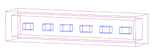
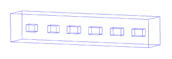
a) $\Omega=\Omega_{FEM}\cup\Omega_{FDM}$	b) $\Omega_{FEM}$

Figure 2: a) The hybrid domain $\Omega=\Omega_{FEM}\cup\Omega_{FDM}$ b) Finite element domain $\Omega_{FEM}$.

The computational geometry $\Omega$ is split into two geometries, $\Omega_{FEM}$ and $\Omega_{FDM}$ such that $\Omega=\Omega_{FEM}\cup\Omega_{FDM}$, see Figure 2. Next, we introduce dimensionless spatial variables $x^{\prime}=x/\left(1m\right)$ and obtain that the domain $\Omega_{FEM}$ is transformed into dimensionless computational domain

$$\Omega_{FEM}=\left\{x=(x_{1},x_{2},x_{3})\in(-3.2,3.2)\times(-0.6,0.6)\times(-0.6,0.6)\right\}.$$

The dimensionless size of our computational domain $\Omega$ for the forward problem is

$$\Omega=\left\{x=(x_{1},x_{2},x_{3})\in(-3.4,3.4)\times(-0.8,0.8)\times(-0.8,0.8)\right\}.$$

The space mesh in $\Omega_{FEM}$ and in $\Omega_{FDM}$ consists of tetrahedral and cubes, respectively. We choose the mesh size $h=0.1$ in our geometries in the hybrid FEM/FDM method, as well as in the overlapping regions between FEM and FDM domains.

In all our computations we use single plane wave $p(t)$ initialized at $\partial_{1}\Omega$ in time $T=[0,3.0]$ such that

$$\begin{split}p\left(t\right)=\left\{\begin{array}[]{ll}\sin\left(\omega t\right),&\text{ if }t\in\left(0,\frac{2\pi}{\omega}\right),\\ 0,&\text{ if }t>\frac{2\pi}{\omega}.\end{array}\right.\end{split}$$ (52)

For generation of simulated backscattered data we define exact function ${a(x)}=4$ inside small scatterers, see Figure 2, and $a(x)=1$ at all other points of the computational domain $\Omega_{FEM}$. Then we solve the forward problem on a refined mesh which is not the same as used in our computations of inverse problem. In a such way we avoid the problem with variational crimes. The time step in all our computations is set to be $\tau=0.006$ which satisfies the CFL condition [20]. Isosurfaces of the simulated solution for the problem (15) with exact function $a(x)$ and $\omega=60$ in (52) are presented in figure 3. Using this figure we observe non-zero behavior of this solution with initialized initial condition (55).

In all our numerical simulations we have considered the additive noise $\sigma$ introduced to the simulated boundary data $\tilde{u}$ in (19). We have performed following reconstruction tests with the same values of parameters in the reconstruction algorithm 3:

• Test 1. Reconstruction of the function $a(x)$ in Model Problem 1 for $\omega\in[20,60]$ in (52) and additive noise levels $\sigma=3\%$ and $\sigma=10\%$.

• Test 2. Reconstruction of the function $a(x)$ in Model Problem 2 for $\omega\in[20,60]$ in (52) and additive noise levels $\sigma=3\%$ and $\sigma=10\%$.

In all our tests we start the algorithm 3 with guess values of the parameter $a(x)=1.0$ at all points in $\Omega$. We refer to [2]-[4], [6, 7] for a similar choice of initial guess which corresponds to starting of the algorithm 3 from the homogeneous domain. The minimal and maximal values of the functions $a(x)$ in our computations belongs to the following set of admissible parameters

$$\begin{split}M_{a}\in\{a\in C(\overline{\Omega})|1\leq a(x)\leq 5\}.\\ \end{split}$$ (53)

We regularize the solution of the inverse problem by computations with single value of the regularization parameter $\gamma=0.01$ in (20). Our computational experience have shown that such choice of $\gamma$ is optimal one in our case. Testing of different techniques, see , for example, [14], of the computing of regularization parameter is the topic of our ongoing research. The tolerance $\theta$ in our algorithm (section 8) is set to $\theta=10^{-6}$.

We use a post-processing procedure to get final images with our reconstructions. This procedure is as follows: assume, that functions $a^{m}(x)$ are our reconstructions obtained by algorithm 3 of section 8 where $m$ is the number of iteration when we have stopped to compute $a(x)$. Then to get post-processed images, we set

$$\widetilde{a}^{m}(x)=\left\{\begin{array}[]{ll}a^{m}(x),&\text{ if }a^{m}(x)>0.6\max\limits_{\Omega_{FEM}}a^{m}(x),\\ 1,&\text{ otherwise. }\end{array}\right.$$ (54)

Results of reconstruction for both tests are presented in tables 1,2. Here, computational errors in procents are computed for $\max\limits_{\Omega_{FEM}}a_{\overline{N}}$, where $\overline{N}:=m$, and are compared with exact ones $a(x)=4$.

Table 1. Results of reconstruction of $a(x)$ for $\sigma=3\%$ together with computational errors in procents. Here, $\overline{N}$ is the final iteration number $m$ in the conjugate gradient method of section 8.

$\sigma=3\%$ $\sigma=3\%$ Test 1 $\max\limits_{\Omega_{FEM}}a_{\overline{N}}$ error, $\%$ $\overline{N}$ $\omega=20$ $5.0$ 25 $7$ $\omega=30$ $5$ 25 $9$ $\omega=40$ $4.73$ 18.3 $10$ $\omega=50$ $5.0$ 25 $11$ $\omega=60$ $5.0$ 25 $12$ Test 2 $\max\limits_{\Omega_{FEM}}a_{\overline{N}}$ error, $\%$ $\overline{N}$ $\omega=20$ $5.0$ 25 $8$ $\omega=30$ $4.86$ 21.5 $9$ $\omega=40$ $4.19$ 4.75 $10$ $\omega=50$ $5.0$ 25 $11$ $\omega=60$ $5.0$ 25 $12$

Table 2. Results of reconstruction of $a(x)$ for $\sigma=10\%$ together with computational errors in procents. Here, $\overline{N}$ is the final iteration number $m$ in the conjugate gradient method of section 8.

$\sigma=10\%$ $\sigma=10\%$ Test 1 $\max\limits_{\Omega_{FEM}}a_{\overline{N}}$ error, $\%$ $\overline{N}$ $\omega=20$ $3.29$ 17.75 $8$ $\omega=30$ $4.94$ 23.5 $10$ $\omega=40$ $4.35$ 8.75 $11$ $\omega=50$ $4.4$ 10 $12$ $\omega=60$ $4.44$ 11 $13$ Test 2 $\max\limits_{\Omega_{FEM}}a_{\overline{N}}$ error, $\%$ $\overline{N}$ $\omega=20$ $3.28$ 18 $8$ $\omega=30$ $4.57$ 14.25 $10$ $\omega=40$ $3.96$ 1 $11$ $\omega=50$ $4.18$ 4.5 $12$ $\omega=60$ $4.46$ 11.5 $13$

9.1 Test 1

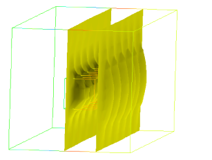
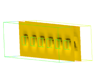
a) $t=1.5$	b) $t=1.5$
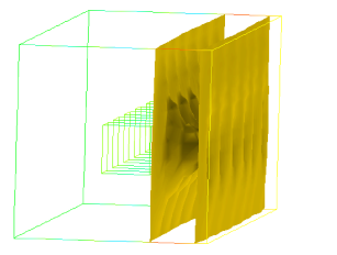
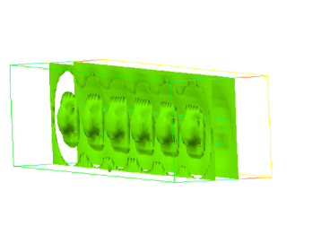
c) $t=1.8$	d) $t=1.8$
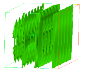
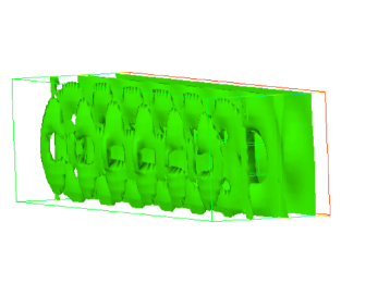
e) $t=2.1$	f) $t=2.1$

Figure 3: Test 1. Isosurfaces of the simulated FEM/FDM solution of the problem (15) with initial conditions (55) in $\Omega_{FEM}$ at different times. On a), c), d) we present transmitted data and on b), d), f) - backscattered data.

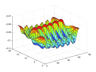
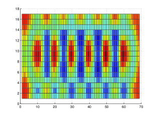
a) Model 1	b) $x_{1}x_{2}$ view
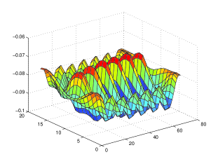
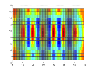
c) Model 2	d) $x_{1}x_{2}$ view
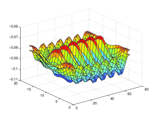
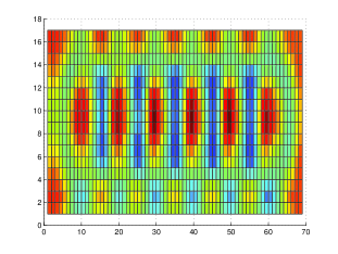
e) Models 1 and 2	f) $x_{1}x_{2}$ view

Figure 4: Test 1. Behavior of noisy backscattered data at time $t=1.8$ in both mathematical models of section 5. Figure e) presents comparison of backscattered data in both models.

To generate backscattered data at the observation points at $S_{T}$ in model problem 1, we solve the forward problem (15), with function $p(t)$ given by (52) in the time interval $t=[0,3.0]$ with the exact values of the parameters $a(x)=4.0$ inside scatterers of figure 2, and $a(x)=1.0$ everywhere else in $\Omega$. We initialized initial conditions at backscattered side $\partial_{1}\Omega$ as

$$\begin{split}u(x,0)&=\exp^{-(x_{1}^{2}+x_{2}^{2}+x_{3}^{3})}\cdot\cos t|_{t=0}=\exp^{-(x_{1}^{2}+x_{2}^{2}+x_{3}^{3})},\\ \frac{\partial u}{\partial t}(x,0)&=-\exp^{-(x_{1}^{2}+x_{2}^{2}+x_{3}^{3})}\cdot\sin t|_{t=0}\equiv 0.\end{split}$$ (55)

Figure 3-a) presents behavior of this initial condition.

Figure 4 presents typical behavior of noisy backscattered data for scatterers of figure 2 in our two models of section 5. Using figure 4-e) we observe that the difference in the amplitude of these two data sets is very small, and thus, we expect that the influence of the non-zero initial conditions will not affect to the reconstructions too much.

Figure 5-a) presents behavior of the computed $L_{2}$ norms of differences $F^{m}=||\delta u^{m}-\delta u^{m-1}||$ for $m>0$, where $\delta u^{m}=||u^{m}-\tilde{u}||z_{\delta}$ for $\omega=40$ in (52) and noise level $\sigma=3\%$. Analyzing this figure for model problem 1 we observe that we achieve convergence in the optimization algorithm at iteration $m=10$ in the conjugate gradient method. Figures 6 presents typical behavior of the computed $L_{2}$ norms of differences $F^{m}=||\delta u^{m}-\delta u^{m-1}||$ for $m>0$, where $\delta u^{m}=||u^{m}-\tilde{u}||z_{\delta}$ for different values of $\omega$ in (52) and noise level $\sigma=10\%$.

We can see results of reconstruction for model problem 1 in tables 1,2. The reconstructed images of the conductivity function for both noise levels and different $\omega$ are presented in figures 7, 9. Figures 7-b) and 9-c) show best results of reconstruction which we have obtained for $\omega=40$. We observe that for the noise $\sigma=3\%$ we get correct locations of scatterers and values of reconstructed parameter $a(x)\approx 4.73$ inside them compared with exact one $c=4.0$. For the noise $\sigma=10\%$ we get correct locations of scatterers and values of reconstructed parameter $a(x)\approx 4.35$ inside them.

Using these figures we observe that the location of all inclusions in $x_{1}x_{2}$ directions is imaged very well. However, from figure 11 follows that the location in $x_{3}$ direction should still be improved.

9.1.1 Test 2

This test is similar to the previous one, only we solve IP2 in this case. We start the optimization algorithm with guess values of the parameters $a(x)=1.0$ at all points in $\Omega$. We use the same as in (53) set of admissible parameters $M_{a}$ and the same regularization procedure as in test 1.

Figure 5-b) presents behavior of the computed $L_{2}$ norms of differences $F^{m}=||\delta u^{m}-\delta u^{m-1}||$, $m>0$, for $\omega=40$ in (52) and noise level $\sigma=3\%$. Analyzing this figure for model problem 2 we observe that we achieve convergence in the optimization algorithm at iteration $m=10$ in the conjugate gradient method. Figure 6-b) presents typical behavior of the computed $L_{2}$ norms of differences $F^{m}=||\delta u^{m}-\delta u^{m-1}||$ for $m>0$, where $\delta u^{m}=||u^{m}-\tilde{u}||z_{\delta}$ for different values of $\omega$ in (52) and noise level $\sigma=10\%$ in this test.

Results of reconstruction of $a(x)$ for model problem 2 are presented in tables 1,2. Figures 8, 10 show results of reconstruction for both noise levels and different $\omega$. Using tables 1,2 we observe that best results of reconstruction are obtained for $\omega=40$. Figures 8-b) and 10-b) show these results. Using figure 8-b) we observe that for the noise $\sigma=3\%$ we get correct locations of scatterers and values of reconstructed parameter $a(x)\approx 4.19$ inside them compared with exact one $a=4.0$ for $\omega=40$. From figure 10-b) we see that for the noise $\sigma=10\%$ we get correct locations of scatterers and values of reconstructed parameter $a(x)\approx 3.96$ inside them for $\omega=40$.

Thus, we again conclude that the location of all inclusions in $x_{1}x_{2}$ directions is imaged very well, but from figure 11 follows that the location in $x_{3}$ direction should still be improved.

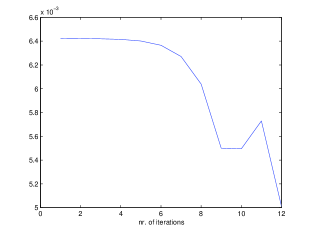
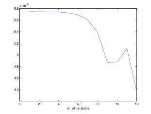
a) Model problem 1	b) Model problem 2

Figure 5: Differences $F^{m}=||\delta u^{m}-\delta u^{m-1}||$ for $\omega=40$ in (52). Noise in backscattered data is 3%.

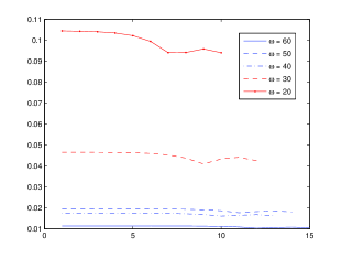
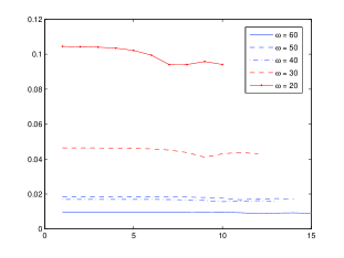
a) Model problem 1	b) Model problem 2

Figure 6: Behavior of differences $F^{m}=||\delta u^{m}-\delta u^{m-1}||$ for Model Problem 1 (left figures) and for Model Problem 2 (right figures). Noise in backscattered data is 10%.

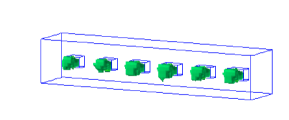
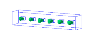
a) $\omega=30,\max\limits_{\Omega_{FEM}}a(x)=5$	b) $\omega=40,\max\limits_{\Omega_{FEM}}a(x)=4.73$
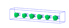
c) $\omega=50,\max\limits_{\Omega_{FEM}}a(x)=5.0$	d) $\omega=60,\max\limits_{\Omega_{FEM}}a(x)=5.0$

Figure 7: Test 1. Computed images of reconstructed functions $a(x)$ in model problem 1. We present functions $\tilde{a}$ for different $\omega$ in (52) and noise level $\sigma=3\%$.

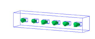
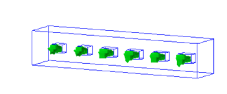
a) $\omega=30,\max\limits_{\Omega_{FEM}}a(x)=4.86$	b) $\omega=40,\max\limits_{\Omega_{FEM}}a(x)=4.19$
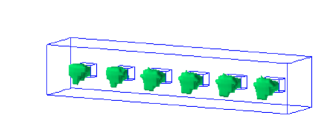
c) $\omega=50,\max\limits_{\Omega_{FEM}}a(x)=5$	d) $\omega=60,\max\limits_{\Omega_{FEM}}a(x)=5$

Figure 8: Test 2. Computed images of reconstructed functions $a(x)$ in model problem 2. We present functions $\tilde{a}$ for different $\omega$ in (52) and noise level $\sigma=3\%$. Here we have initialized zero boundary conditions in the generation of backscattered data and in the optimization algorithm.

a) $\omega=20,\max\limits_{\Omega_{FEM}}a(x)=3.29$	b) $\omega=30,\max\limits_{\Omega_{FEM}}a(x)=4.94$
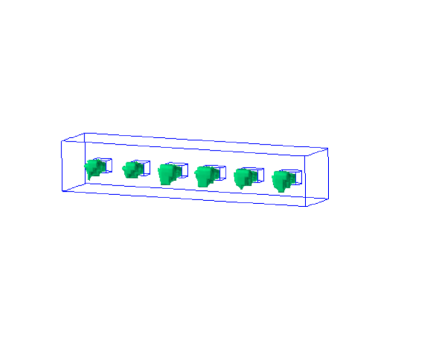
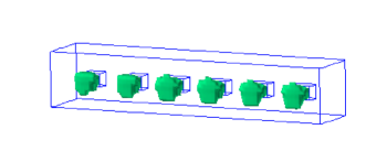
c) $\omega=40,\max\limits_{\Omega_{FEM}}a(x)=4.35$	d) $\omega=50,\max\limits_{\Omega_{FEM}}a(x)=4.4$

Figure 9: Test 1. Computed images of reconstructed functions $a(x)$ in model problem 1. We present functions $\tilde{a}$ for different $\omega$ in (52) and noise level $\sigma=10\%$.

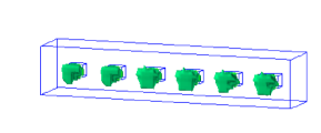
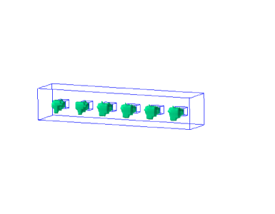
a) $\omega=30,\max\limits_{\Omega_{FEM}}a(x)=4.57$	b) $\omega=40,\max\limits_{\Omega_{FEM}}a(x)=3.96$
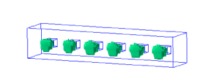
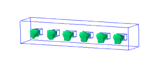
c) $\omega=50,\max\limits_{\Omega_{FEM}}a(x)=4.18$	d) $\omega=60,\max\limits_{\Omega_{FEM}}a(x)=4.46$

Figure 10: Test 2. Computed images of reconstructed functions $a(x)$ in model problem 2. We present functions $\tilde{a}$ for different $\omega$ in (52) and noise level $\sigma=10\%$.

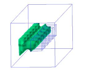
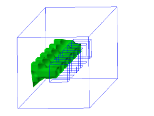
e) Test 1: $\omega=40,\sigma=10\%$	f) Test 2: $\omega=40,\sigma=3\%$

Figure 11: Computed images of reconstructed functions $a(x)$ in both model problems. We present functions $\tilde{a}$ for $\omega=40$ in (52). We observe that reconstruction in $x_{3}$ direction should be improved.

10 Discussion and Conclusion

In this work we present domain decomposition FEM/FDM method which is applied for reconstruction of the conductivity function in the hyperbolic equation in three dimensions. We have formulated inverse problems and presented Lagrangian approach to solve these problems. Explicit schemes for the solution of forward and adjoint problems in the domain decomposition approach are also derived. We have formulated different domain decomposition algorithms: the algorithm 1 describes the overlapping procedure between finite element and finite difference domains, the algorithm 2 presents solution of the forward and adjoint problems using the domain decomposition FEM/FDM methods, and the algorithm 3 describes the conjugate gradient algorithm for reconstruction of the conductivity function with usage of algorithms 1,2.

In our numerical tests we have obtained stable and good reconstruction of the conductivity function $a(x)$ in the range of frequencies $\omega\in[20,60]$ . Using tables 1,2 we can conclude that the best reconstruction results are obtained in model problem 2 for $\omega=40$. We can also conclude that in all tests we could reconstruct size on $x_{1}x_{2}$ -directions for $a$, however, size in $x_{3}$ direction should be still improved. Similarly with [2, 6, 7] we plan to apply an adaptive finite element method in order to get better shapes and sizes of the inclusions in all directions.

References

- [1] F. Assous, P. Degond, E. Heintze and P. Raviart, On a finite-element method for solving the three-dimensional Maxwell equations, J. Comput. Physics, 109 (1993), 222–237.
- [2] L. Beilina, Adaptive hybrid FEM/FDM methods for inverse scattering problems. Inverse Problems and Information Technologies, V.1, N.3, pp.73-116, 2002.
- [3] L. Beilina, M. Cristofol and K. Niinimäki, Optimization approach for the simultaneous reconstruction of the dielectric permittivity and magnetic permeability functions from limited observations, Inverse Problems and Imaging, 9 (1), pp. 1-25, 2015
- [4] L. Beilina, Energy estimates and numerical verification of the stabilized Domain Decomposition Finite Element/Finite Difference approach for time-dependent Maxwell’s system, Cent. Eur. J. Math., 11 (2013), 702-733 DOI: 10.2478/s11533-013-0202-3.
- [5] L. Beilina, K. Samuelsson, K. Åhlander, Efficiency of a hybrid method for the wave equation. Proceedings of the International Conference on Finite Element Methods: Three dimensional problems. GAKUTO international Series, Mathematical Sciences and Applications, V. 15, 2001.
- [6] L. Beilina, Adaptive Hybrid Finite Element/Difference method for Maxwell’s equations: an a priory error estimate and efficiency, Applied and Computational Mathematics (ACM), 9 (2) s. 176-197, 2010.
- [7] L. Beilina and C. Johnson, A posteriori error estimation in computational inverse scattering, Mathematical Models in Applied Sciences, 1, 23-35, 2005.
- [8] S. C. Brenner and L. R. Scott, The Mathematical theory of finite element methods, Springer-Verlag, Berlin, 1994.
- [9] T. Chan and T. Mathew, Domain decomposition algorithms, In A. Iserles, editor, Acta Numerica, V. 3, Cambridge University Press, Cambridge, UK, 1994.
- [10] A. Toselli, B. Widlund, Domain decomposition methods, Springer, 2005.
- [11] G. C. Cohen, Higher order numerical methods for transient wave equations, Springer-Verlag, 2002.
- [12] M. Cristofol, S. Li, E. Soccorsi, Determining the waveguide conductivity in a hyperbolic equation from a single measurement on the lateral boundary, arXiv: 1501,01384, 2015.
- [13] Engquist B and Majda A, Absorbing boundary conditions for the numerical simulation of waves Math. Comp. 31, pp.629-651, 1977.
- [14] H. W. Engl, M. Hanke and A. Neubauer, Regularization of Inverse Problems (Boston: Kluwer Academic Publishers), 2000.
- [15] O. A. Ladyzhenskaya, Boundary Value Problems of Mathematical Physics, Springer Verlag, Berlin, 1985.
- [16] PETSc, Portable, Extensible Toolkit for Scientific Computation, http://www.mcs.anl.gov/petsc/
- [17] O.Pironneau, Optimal shape design for elliptic systems, Springer-Verlag, Berlin, 1984.
- [18] A. N. Tikhonov, A. V. Goncharsky, V. V. Stepanov and A. G. Yagola, Numerical Methods for the Solution of Ill-Posed Problems (London: Kluwer), 1995.
- [19] WavES, the software package, http://www.waves24.com
- [20] R. Courant, K. Friedrichs and H. Lewy On the partial differential equations od mathematical physics, IBM Journal of Research and Development, 11(2) (1967), 215-234