Limit behaviour of the truncated pathwise Fourier-transformation of Lévy-driven CARMA processes for non-equidistant discrete time observations

Żywilla Fechner 1,2 and Robert Stelzer 2 1 Institute of Mathematics, University of Silesia, Bankowa 14, 40-007 Katowice, Poland
2 Institute of Mathematical Finance, Ulm University, Helmholtzstraße 18, 89069 Ulm, Germany
zfechner@gmail.com, robert.stelzer@uni-ulm.de
Abstract.

This paper considers a continuous time analogue of the classical autoregressive moving average processes, Lévy-driven CARMA processes. First we describe limiting properties of the periodogram by means of the so-called truncated Fourier transform if observations are available continuously. The obtained results are in accordance with their counterparts from the discrete-time case. Then we discuss the numerical approximation of the truncated Fourier transform based on non-equidistant high frequency data. In order to ensure convergence of the numerical approximation to the true value of the truncated Fourier transform a certain control on the maximal distance between observations and the number of observations is needed. We obtain both convergence to the continuous time quantity and asymptotic normality under a high-frequency infinite time horizon limit.

Key words and phrases:
CARMA Process, Frequency Domain, High-frequency Data, Lévy Process, Trapezoidal Rule
2010 Mathematics Subject Classification:
Primary 62M10, 62M15, Secondary 60G10, 60G51

1. Introduction

The classical autoregressive moving average process ARMAARMA\operatorname{ARMA} has been broadly discussed in the literature. For a comprehensive discussion see e.g. the monograph by Brockwell and Davis [BrockwellDavis] and references therein. In the discrete time models we restrict ourselves to observations at fixed equidistant points in time. In many cases these observations made at discrete times come from an underlying continuous process, thus the natural question arises: can we model also the time series in continuous time? One of the earliest results dealing with properties of such processes can be found in Doob [Doob]. Later this problem was discussed by Brockwell in [Brockwell2001a] for continuous time ARMAARMA\operatorname{ARMA} processes driven by Gaussian noise. The next step was to extend these ideas to the models with noise modelled by jump processes, so-called Lévy-driven CARMACARMA\operatorname{CARMA} models introduced by Brockwell in [Brockwell2001]. In these papers time series are modelled as continuous time processes with continuous time noises (with or without jumps) and the inference is based mainly on discrete equidistant data. One of the latest results can be found in the paper [BrockwellDavisYang] of Brockwell, Davis and Yang, which consideres QML estimations of the ARAR\operatorname{AR} and MAMA\operatorname{MA} parameters based on equidistant observations.

The estimation procedure of Lévy-driven CARMACARMA\operatorname{CARMA} processes in high-frequency settings has been discussed by Fasen and Fuchs in [FuchsFasen2013], where the authors deal with the limit behaviour of the periodogram of CARMACARMA\operatorname{CARMA} processes under equidistant sampling when the sampling interval tends to 00. The results are analogous to ARMAARMA\operatorname{ARMA} processes: the periodogram for CARMACARMA\operatorname{CARMA} processes is not a consistent estimator of the spectral density function, but after appropriate smoothing the consistency can be obtained. Some related results were discussed by Fasen and Fuchs in [FuchsFasen2013a], where asymptotic distributions of periodograms of CARMACARMA\operatorname{CARMA} processes driven by a symmetric α𝛼\alpha-stable Lévy noise are obtained and where it is shown that the vector composed of periodograms for various frequencies converges in distribution to a function of a multidimensional stable random vector. Likewise, Fasen [Fasen2013] considers the behaviour of the periodogram for an equidistantly sampled continuous time moving average process when only the number of observations goes to infinity.

The problem of statistical analysis of such processes has been studied further for example by Gillberg in his dissertation [Gillberg2006], where different approaches to the estimation of CARMACARMA\operatorname{CARMA} processes with Gaussian noise are discussed both using equidistant and non-equidistant observations. The author works mainly in the frequency domain. He describes the properties of the truncated Fourier transform of a CARMACARMA\operatorname{CARMA} process with Gaussian noise on a fixed interval [0,T]0𝑇[0,T] based on equidistant frequencies. In the non-equidistant case he has used a method based on splines in order to find an approximation of the spectral density.

Another approach for the estimation of a zero-mean stationary process (Yt)tsubscriptsubscript𝑌𝑡𝑡(Y_{t})_{t\in\mathbb{R}} with finite second-order moments and continuous covariance function has been discussed by Lii and Masry in [LiiMasry1992] and [LiiMasry1994], where they described some properties of a smoothed periodogram. Here observations are assumed to be given on a random grid (τk)subscript𝜏𝑘(\tau_{k}) of an interval [0,T]0𝑇[0,T], where τksubscript𝜏𝑘\tau_{k} is a stationary point process on the real line which is independent of (Yt)tsubscriptsubscript𝑌𝑡𝑡(Y_{t})_{t\in\mathbb{R}}.

In the present paper we are going to describe the asymptotic behaviour of the so-called truncated Fourier transform of a CARMACARMA\operatorname{CARMA} process, which is a building block for an estimation of the spectral density of a CARMACARMA\operatorname{CARMA} process. We are going to use some of the ideas from [Gillberg2006] to prove results in more general settings.

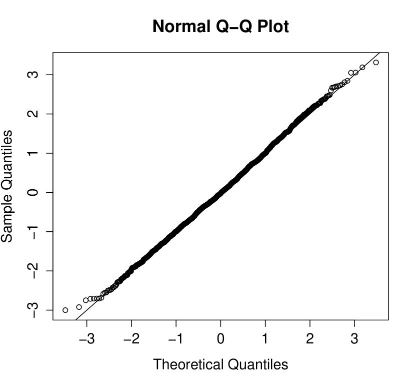
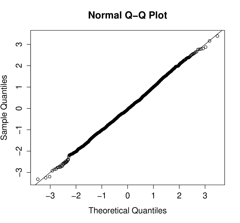
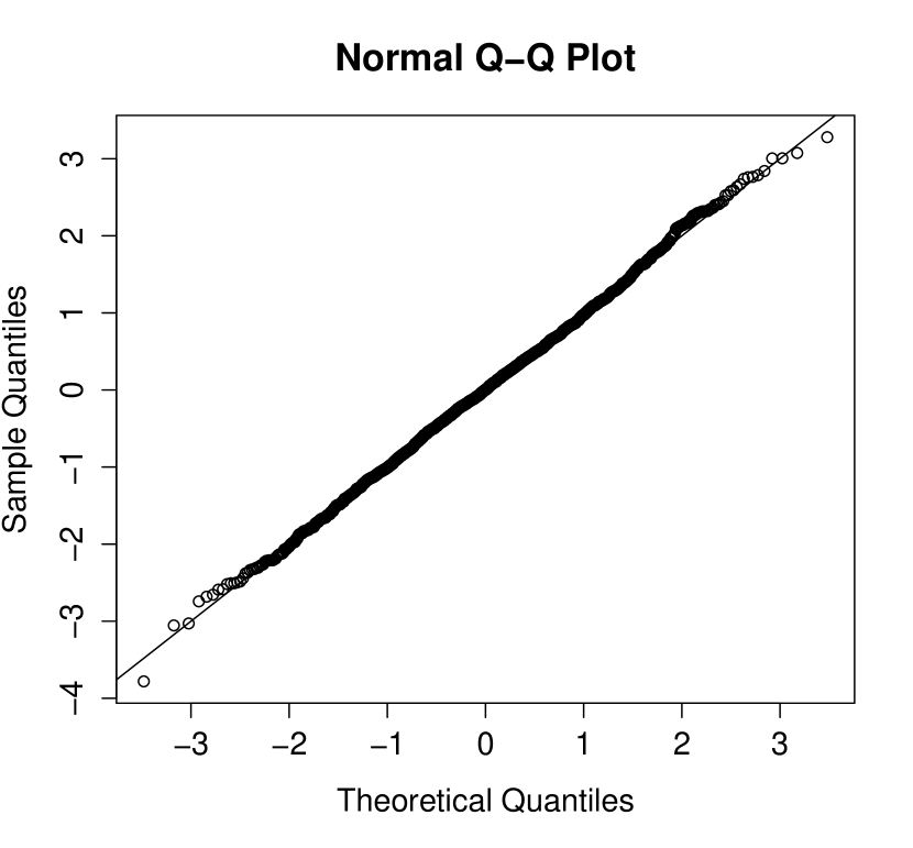
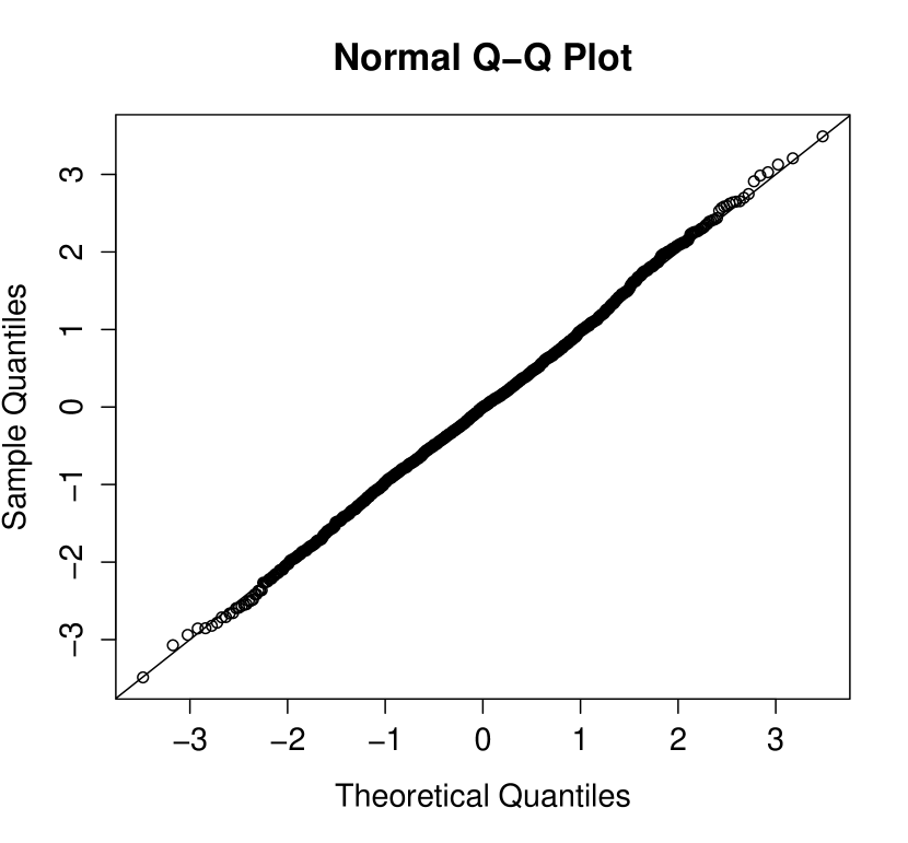
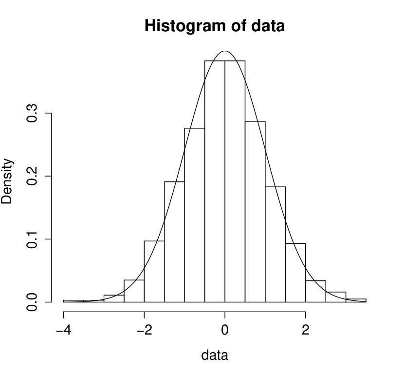
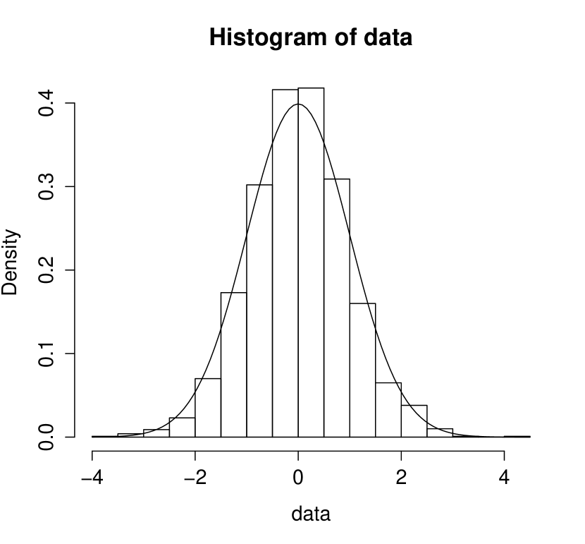
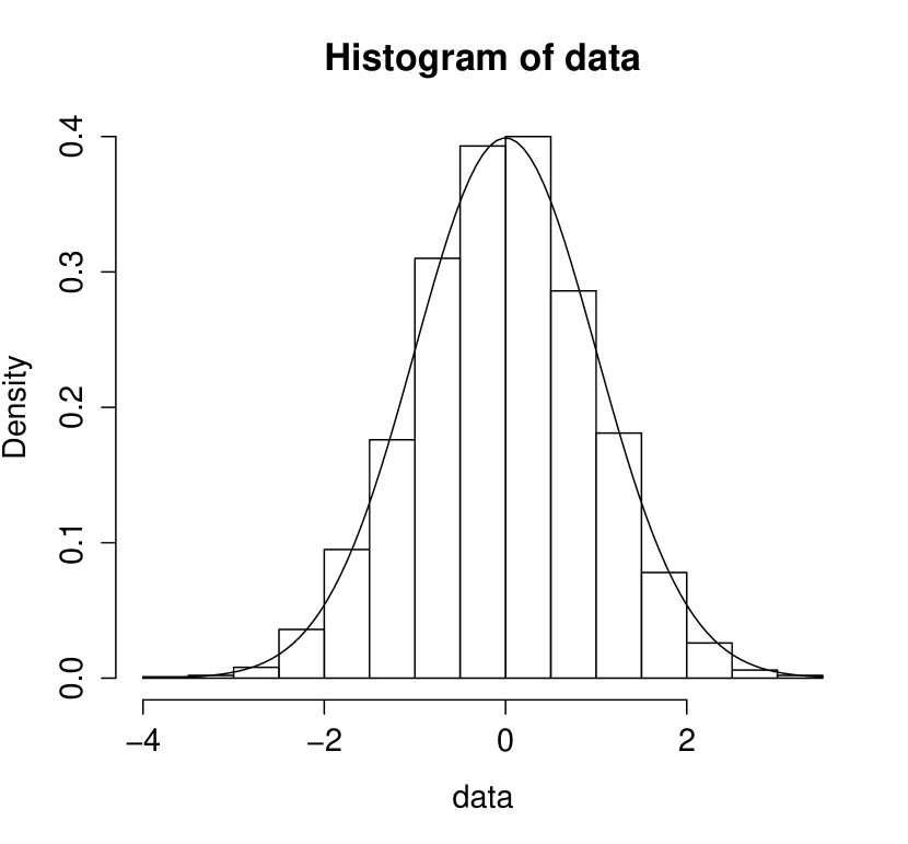
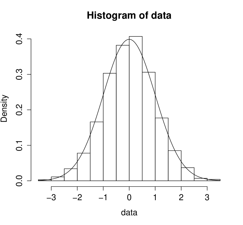
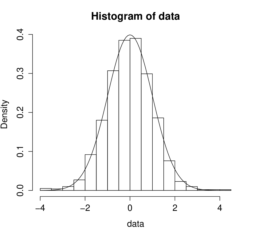
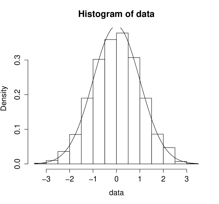
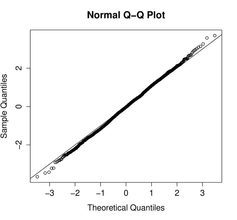
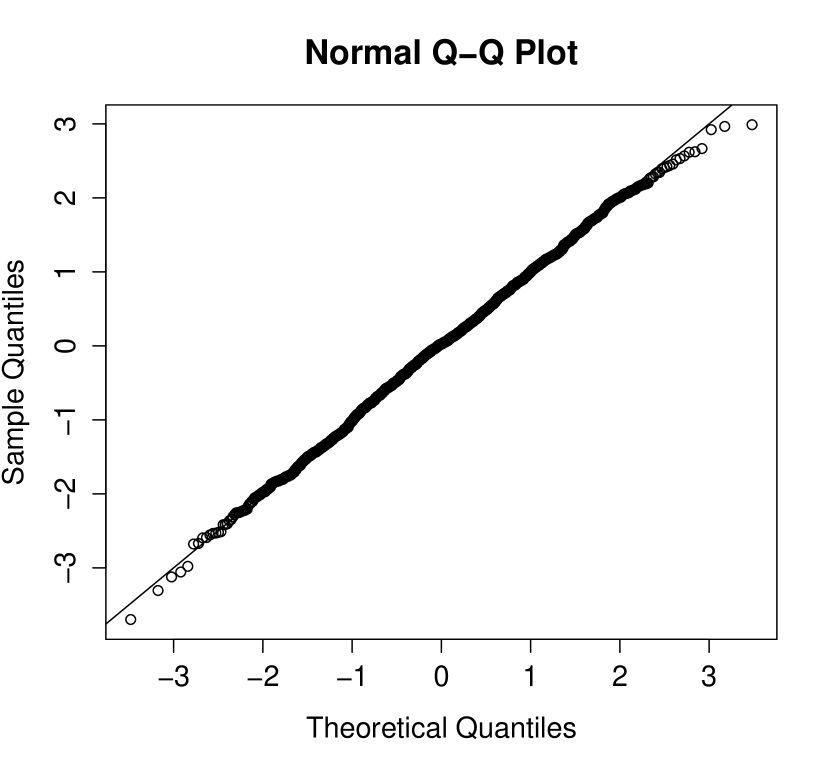
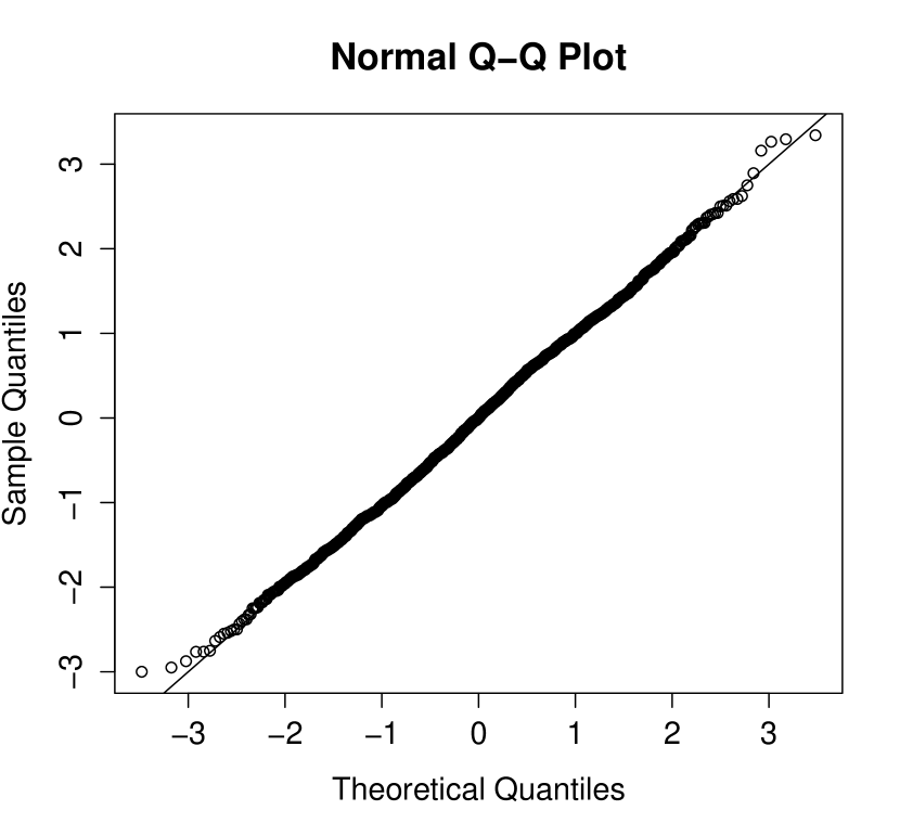
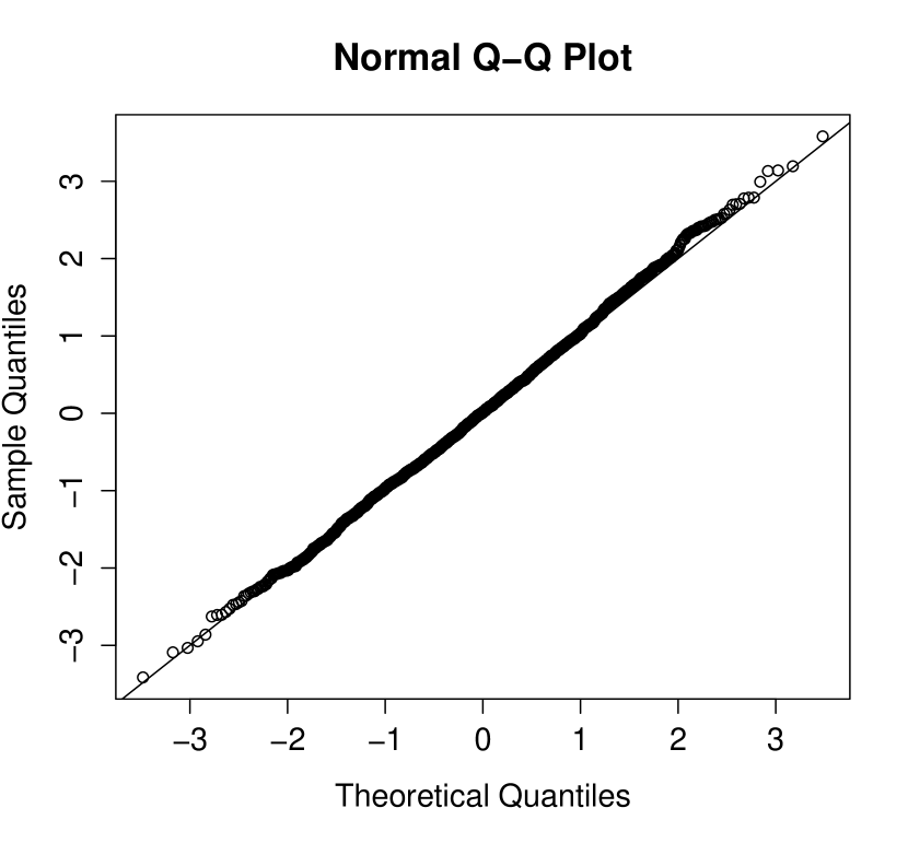
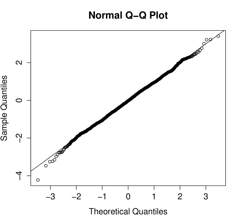
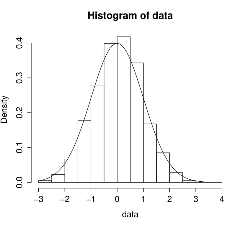
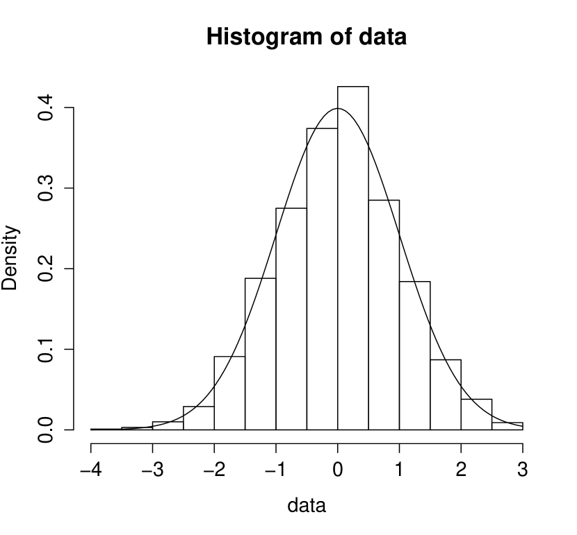
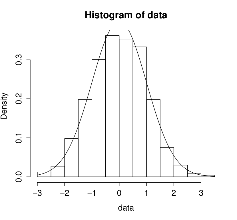
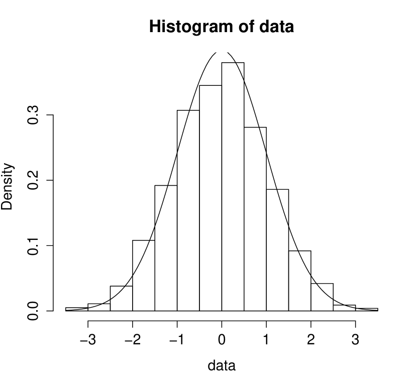
The paper is structured as follows: first we recall second order Lévy-driven CARMACARMA\operatorname{CARMA} models and summarize the results needed later in Section 2. Then we define in Section 3 the truncated Fourier transform of a CARMACARMA\operatorname{CARMA} process and we investigate its asymptotic properties at a fixed frequency: for a non-zero frequency we obtain that the limiting law of the real and imaginary part is the two dimensional normal distribution with mean zero and the covariance matrix depending on the spectral density of the CARMACARMA\operatorname{CARMA} process. If we consider the truncated Fourier transform at zero, we obtain a one dimensional normal law with mean zero and variance depending only on two parameters of the CARMACARMA\operatorname{CARMA} process. We show that the limiting law of the joint distribution of the squared modulus of the truncated Fourier transform at different positive frequencies converges to a vector of independent and exponentially distributed random variables with mean depending on the values of the spectral density. All these results can be interpreted as the limiting behaviour of the truncated Fourier transform when the CARMACARMA\operatorname{CARMA} process is observed continuously. The next step in Section 3.2 is to approximate the truncated Fourier transform when the CARMACARMA\operatorname{CARMA} process is observed on a non-equidistant deterministic grid. In order to find a numerical approximation value of the truncated Fourier transform we apply the trapezoidal rule. We are interested in the convergence of the truncated Fourier transform when the length of the interval T𝑇T goes to infinity and the mesh of the grid to zero. Since the interplay of the length of the interval, of the number of elements of the grid and of the maximal distance between the elements of the grid plays a crucial role, in order to ensure the convergence of the approximating sum to the true value of the truncated Fourier transform we have to impose some limiting conditions on these quantities. In the last Section 4 we look at some illustrative simulations of the truncated Fourier transform based on non-equidistant observations. We consider Ornstein-Uhlenbeck type (CAR(1)) and CARMA(2,1) processes driven by a standard Brownian motion, a Variance Gamma process and a “two-sided Poisson process” and we compare our simulations with the theoretical asymptotic distributions described earlier.

Notation

The symbol :={1,2,3,}assign123\mathbb{N}:=\{1,2,3,\dots\} denotes the set of positive integers, 0:={0}assignsubscript00\mathbb{N}_{0}:=\mathbb{N}\cup\{0\}, \mathbb{R} is the set of real numbers and \mathbb{C} denotes the set of complex numbers. The symbol m×nsuperscript𝑚𝑛\mathbb{R}^{m\times n}, resp. m×nsuperscript𝑚𝑛\mathbb{C}^{m\times n} denotes the space of real- (resp. complex-) valued matrices with m𝑚m rows and n𝑛n columns. For Am×n𝐴superscript𝑚𝑛A\in\mathbb{C}^{m\times n} the symbol ATsuperscript𝐴𝑇A^{T} denotes the transposed of a matrix A𝐴A. We are working on a given filtered probability space (Ω,,(t)t0,)Ωsubscriptsubscript𝑡𝑡0(\Omega,\mathcal{F},(\mathcal{F}_{t})_{t\geq 0},\mathbb{P}) satisfying the usual hypothesis (cf. Protter [Protter], Chapter 1).

Moreover, by X=dYsuperscript𝑑𝑋𝑌X\stackrel{{\scriptstyle d}}{{=}}Y we denote that the random variables X𝑋X and Y𝑌Y are equal in distribution.

2. Preliminaries

We begin with the model set-up given by Brockwell (see [Brockwell2001], [Brockwell2001a]). A second-order Lévy-driven continuous-time ARMA(p,q)ARMA𝑝𝑞\operatorname{ARMA}(p,q) process is defined in terms of a state-space representation of the formal differential equation

(1) a(D)Y(t)=b(D)DL(t),t0.formulae-sequence𝑎𝐷𝑌𝑡𝑏𝐷𝐷𝐿𝑡𝑡0a(D)Y(t)=b(D)DL(t),\quad t\geq 0.

Here, D𝐷D denotes differentiation with respect to t𝑡t, non-negative integers p,q𝑝𝑞p,q satisfying p>q𝑝𝑞p>q and (L(t))t0subscript𝐿𝑡𝑡0(L(t))_{t\geq 0} is a one dimensional Lévy process (i.e. a continuous time process with stationary and independent increments and L(0)=0𝐿00L(0)=0 a.s.) with 𝔼L(1)2<𝔼𝐿superscript12\mathbb{E}L(1)^{2}<\infty. A comprehensive monograph dealing with Lévy processes is e.g. [Applebaum2009]. The polynomials

a(z):=zp+a1zp1++ap,b(z):=b0+b1z++bp1zp1,formulae-sequenceassign𝑎𝑧superscript𝑧𝑝subscript𝑎1superscript𝑧𝑝1subscript𝑎𝑝assign𝑏𝑧subscript𝑏0subscript𝑏1𝑧subscript𝑏𝑝1superscript𝑧𝑝1a(z):=z^{p}+a_{1}z^{p-1}+\dots+a_{p},\quad b(z):=b_{0}+b_{1}z+\dots+b_{p-1}z^{p-1},

are called the autoregressive- and moving average polynomial, respectively. We assume that bq0subscript𝑏𝑞0b_{q}\neq 0 and bj=0subscript𝑏𝑗0b_{j}=0 for q<j<p𝑞𝑗𝑝q<j<p. The state-space representation consists of the observation and state equations:

(2) Y(t)=𝐛T𝐗(t),𝑌𝑡superscript𝐛𝑇𝐗𝑡Y(t)=\mathbf{b}^{T}\mathbf{X}(t),
(3) d𝐗(t)=𝐀𝐗(t)dt+𝐞dL(t),𝑑𝐗𝑡𝐀𝐗𝑡𝑑𝑡𝐞𝑑𝐿𝑡d\mathbf{X}(t)=\mathbf{A}\mathbf{X}(t)dt+\mathbf{e}dL(t),

where

𝐀:=[010000100001apap1ap2a1],𝐗(t):=[X(t)X(1)(t)X(p2)(t)X(p1)(t)],formulae-sequenceassign𝐀delimited-[]matrix010000100001subscript𝑎𝑝subscript𝑎𝑝1subscript𝑎𝑝2subscript𝑎1assign𝐗𝑡delimited-[]matrix𝑋𝑡superscript𝑋1𝑡superscript𝑋𝑝2𝑡superscript𝑋𝑝1𝑡\mathbf{A}:=\left[\begin{matrix}0&1&0&\ldots&0\\ 0&0&1&\ldots&0\\ \vdots&\vdots&\vdots&\ddots&\vdots\\ 0&0&0&\ldots&1\\ -a_{p}&-a_{p-1}&-a_{p-2}&\ldots&-a_{1}\\ \end{matrix}\right],\quad\mathbf{X}(t):=\left[\begin{matrix}X(t)\\ X^{(1)}(t)\\ \vdots\\ X^{(p-2)}(t)\\ X^{(p-1)}(t)\\ \end{matrix}\right],\quad
𝐞:=[0,0,1]T,𝐛:=[b0,b1,bp1]T,formulae-sequenceassign𝐞superscript001𝑇assign𝐛superscriptsubscript𝑏0subscript𝑏1subscript𝑏𝑝1𝑇\mathbf{e}:=\left[0,\dots 0,1\right]^{T},\quad\mathbf{b}:=\left[b_{0},b_{1},\dots b_{p-1}\right]^{T},

i.e.

𝐀p×p,𝐗(t)p×1𝐞p,𝐛p.formulae-sequence𝐀superscript𝑝𝑝formulae-sequence𝐗𝑡superscript𝑝1formulae-sequence𝐞superscript𝑝𝐛superscript𝑝\mathbf{A}\in\mathbb{R}^{p\times p},\quad\mathbf{X}(t)\in\mathbb{R}^{p\times 1}\quad\mathbf{e}\in\mathbb{R}^{p},\quad\mathbf{b}\in\mathbb{R}^{p}.

If p=1𝑝1p=1, we set 𝐀=a1𝐀subscript𝑎1\mathbf{A}=-a_{1}.

Assumption 2.1.

The Lévy process satisfies 𝔼L(1)=0𝔼𝐿10\mathbb{E}L(1)=0 and 𝔼|L(1)|2=σ2<𝔼superscript𝐿12superscript𝜎2\mathbb{E}|L(1)|^{2}=\sigma^{2}<\infty.

Observe that 𝔼[L(s)L(t)]=min{s,t}𝔼|L(1)|2𝔼delimited-[]𝐿𝑠𝐿𝑡𝑠𝑡𝔼superscript𝐿12\mathbb{E}[L(s)L(t)]=\min\{s,t\}\mathbb{E}|L(1)|^{2}. It was shown by Brockwell in [Brockwell2009] that the solution 𝐗(t)𝐗𝑡\mathbf{X}(t) of (3) satisfies

(4) 𝐗(t)=e𝐀t𝐗(0)+0te𝐀(tu)𝐞𝑑L(u),𝐗𝑡superscript𝑒𝐀𝑡𝐗0superscriptsubscript0𝑡superscript𝑒𝐀𝑡𝑢𝐞differential-d𝐿𝑢\mathbf{X}(t)=e^{\mathbf{A}t}\mathbf{X}(0)+\int_{0}^{t}e^{\mathbf{A}(t-u)}\mathbf{e}dL(u),

where the integral is defined as the L2superscript𝐿2L^{2}-limit of approximating Riemann sums.

Assumption 2.2.

𝐗(0)𝐗0\mathbf{X}(0) is independent of (L(t))t0subscript𝐿𝑡𝑡0(L(t))_{t\geq 0}.

From now on let us assume that Assumption 2.2 holds. It is well-known ([Brockwell2009, Proposition 2]) that under Assumptions 2.1 and 2.2 the process {𝐗(t)}t0subscript𝐗𝑡𝑡0\{\mathbf{X}(t)\}_{t\geq 0} is strictly stationary and causal iff 𝐗(0)𝐗0\mathbf{X}(0) has the same distribution as 0e𝐀u𝐞𝑑L(u)superscriptsubscript0superscript𝑒𝐀𝑢𝐞differential-d𝐿𝑢\int_{0}^{\infty}e^{\mathbf{A}u}\mathbf{e}dL(u) and the p𝑝p (not necessarily distinct) eigenvalues λ1,,λpsubscript𝜆1subscript𝜆𝑝\lambda_{1},\dots,\lambda_{p} of 𝐀𝐀\mathbf{A} have negative real parts, i.e.

(λi)<0,i=1,,p.formulae-sequencesubscript𝜆𝑖0𝑖1𝑝\Re(\lambda_{i})<0,\quad i=1,\dots,p.

Now we extend the Lévy process (L(u))u0subscript𝐿𝑢𝑢0(L(u))_{u\geq 0} to the whole line in the usual way: Let L~=(L~(t))t0~𝐿subscript~𝐿𝑡𝑡0\widetilde{L}=(\widetilde{L}(t))_{t\geq 0} be an independent copy of (L(t))t0subscript𝐿𝑡𝑡0(L(t))_{t\geq 0}. For t𝑡t\in\mathbb{R} we define

L(t):=L(t)𝟙[0,)(t)+L~(t)𝟙(,0](t).assignsuperscript𝐿𝑡𝐿𝑡subscript10𝑡~𝐿limit-from𝑡subscript10𝑡L^{*}(t):=L(t)\mathds{1}_{[0,\infty)}(t)+\widetilde{L}(-t-)\mathds{1}_{(-\infty,0]}(t).

In order to get stationary solutions of (3) we need the following assumptions:

Assumption 2.3.

All eigenvalues of 𝐀𝐀\mathbf{A} have strictly negative real parts.

Assumption 2.4.
𝐗(0)=d0e𝐀u𝐞𝑑L(u)superscript𝑑𝐗0superscriptsubscript0superscript𝑒𝐀𝑢𝐞differential-dsuperscript𝐿𝑢\mathbf{X}(0)\stackrel{{\scriptstyle d}}{{=}}\int_{-\infty}^{0}e^{-\mathbf{A}u}\mathbf{e}dL^{*}(u)

In Brockwell [Brockwell2009] it was shown that if Assumptions 2.3 and 2.4 are satisfied the process {𝐗(t)}tsubscript𝐗𝑡𝑡\{\mathbf{X}(t)\}_{t\in\mathbb{R}} given by

(5) 𝐗(t)=te𝐀(tu)𝐞𝑑L(u)𝐗𝑡superscriptsubscript𝑡superscript𝑒𝐀𝑡𝑢𝐞differential-dsuperscript𝐿𝑢\mathbf{X}(t)=\int_{-\infty}^{t}e^{\mathbf{A}(t-u)}\mathbf{e}dL^{*}(u)

is a strictly stationary solution of (3) (with L𝐿L replaced by Lsuperscript𝐿L^{*}) for t𝑡t\in\mathbb{R} with corresponding CARMACARMA\operatorname{CARMA} process

(6) Y(t)=t𝐛Te𝐀(tu)𝐞𝑑L(u).𝑌𝑡superscriptsubscript𝑡superscript𝐛𝑇superscript𝑒𝐀𝑡𝑢𝐞differential-dsuperscript𝐿𝑢Y(t)=\int_{-\infty}^{t}\mathbf{b}^{T}e^{\mathbf{A}(t-u)}\mathbf{e}dL^{*}(u).

For t0𝑡0t\geq 0 one can rewrite it in the following form

(7) Y(t)=𝐛Te𝐀t𝐗(0)+0t𝐛Te𝐀(tu)𝐞𝑑L(u).𝑌𝑡superscript𝐛𝑇superscript𝑒𝐀𝑡𝐗0superscriptsubscript0𝑡superscript𝐛𝑇superscript𝑒𝐀𝑡𝑢𝐞differential-d𝐿𝑢Y(t)=\mathbf{b}^{T}e^{\mathbf{A}t}\mathbf{X}(0)+\int_{0}^{t}\mathbf{b}^{T}e^{\mathbf{A}(t-u)}\mathbf{e}dL(u).

In the present paper the spectral density of a CARMACARMA\operatorname{CARMA} process plays a crucial role. The spectral density is the Fourier transform of the autocovariance function γY(h):=ov(Y(0),Y(h))assignsubscript𝛾𝑌ov𝑌0𝑌\gamma_{Y}(h):=\mathbb{C}\mathrm{ov}(Y(0),Y(h)) for hh\in\mathbb{R}. The spectral density of a CARMACARMA\operatorname{CARMA} process is

(8) fY(ω)=12πγY(h)eihω𝑑h=σ22π|b(iω)|2|a(iω)|2,ω.formulae-sequencesubscript𝑓𝑌𝜔12𝜋superscriptsubscriptsubscript𝛾𝑌superscript𝑒𝑖𝜔differential-dsuperscript𝜎22𝜋superscript𝑏𝑖𝜔2superscript𝑎𝑖𝜔2𝜔f_{Y}(\omega)=\frac{1}{2\pi}\int_{-\infty}^{\infty}\gamma_{Y}(h)e^{-ih\omega}dh=\frac{\sigma^{2}}{2\pi}\frac{|b(i\omega)|^{2}}{|a(i\omega)|^{2}},\quad\omega\in\mathbb{R}.

3. Limit behaviour of the Fourier transform

In this section we are going to deal with the Fourier transform of the CARMACARMA\operatorname{CARMA} process assuming that the observations are given continuously on the time interval [0,T]0𝑇[0,T]. A similar idea for Gaussian CARMACARMA\operatorname{CARMA} processes was presented in [Gillberg2006] for equidistant observations. The truncated continuous-time Fourier transform of the process Y𝑌Y at a fixed frequency ω𝜔\omega\in\mathbb{R} is given by

T(Y)(ω):=1T0TY(t)eiωt𝑑t.assignsubscript𝑇𝑌𝜔1𝑇superscriptsubscript0𝑇𝑌𝑡superscript𝑒𝑖𝜔𝑡differential-d𝑡\mathcal{F}_{T}(Y)(\omega):=\frac{1}{\sqrt{T}}\int_{0}^{T}Y(t)e^{-i\omega t}dt.

Observe that the norming constant 1T1𝑇\frac{1}{\sqrt{T}} is taken as this ensures convergence in distribution for T𝑇T\to\infty as will be shown later.

3.1. Properties of the Truncated Fourier Transform of a CARMACARMA\operatorname{CARMA} Process

First we derive an alternative representation.

Lemma 3.1.

Let 𝐗𝐗\mathbf{X} and Y𝑌Y be processes given by the state-space representation (2) and (3). Suppose that Assumptions 2.1, 2.2 and 2.3 are satisfied. Then the truncated Fourier transform of the CARMACARMA\operatorname{CARMA} process Y𝑌Y at a fixed frequency ω𝜔\omega\in\mathbb{R} is of the form

(9) T(Y)(ω)=1Tb(iω)a(iω)0Teiωt𝑑L(t)+1T𝐛T(iωIA)1(𝐗(0)eiωT𝐗(T)),subscript𝑇𝑌𝜔1𝑇𝑏𝑖𝜔𝑎𝑖𝜔superscriptsubscript0𝑇superscript𝑒𝑖𝜔𝑡differential-d𝐿𝑡1𝑇superscript𝐛𝑇superscript𝑖𝜔𝐼𝐴1𝐗0superscript𝑒𝑖𝜔𝑇𝐗𝑇\mathcal{F}_{T}(Y)(\omega)=\frac{1}{\sqrt{T}}\frac{b(i\omega)}{a(i\omega)}\int_{0}^{T}e^{-i\omega t}dL(t)+\frac{1}{\sqrt{T}}\mathbf{b}^{T}(i\omega I-A)^{-1}\left(\mathbf{X}(0)-e^{-i\omega T}\mathbf{X}(T)\right),

or equivalently

(10) T(Y)(ω)=subscript𝑇𝑌𝜔absent\displaystyle\mathcal{F}_{T}(Y)(\omega)= 1T𝐛T(iωIA)11𝑇superscript𝐛𝑇superscript𝑖𝜔𝐼𝐴1\displaystyle\frac{1}{\sqrt{T}}\mathbf{b}^{T}(i\omega I-A)^{-1}
×[0T(eiωueiωTe𝐀(Tu))𝐞𝑑L(u)+(Ie(iωI+𝐀)T)𝐗(0)].absentdelimited-[]superscriptsubscript0𝑇superscript𝑒𝑖𝜔𝑢superscript𝑒𝑖𝜔𝑇superscript𝑒𝐀𝑇𝑢𝐞differential-d𝐿𝑢𝐼superscript𝑒𝑖𝜔𝐼𝐀𝑇𝐗0\displaystyle\times\left[\int_{0}^{T}\left(e^{-i\omega u}-e^{-i\omega T}e^{\mathbf{A}(T-u)}\right)\mathbf{e}dL(u)+\left(I-e^{(-i\omega I+\mathbf{A})T}\right)\mathbf{X}(0)\right].

Proof. Let ω𝜔\omega be an arbitrary frequency. Observe that by Corollary 3.4 from [SchlemmStelzer2012, p. 51] one has

𝐛T(𝐀iωI)1𝐞=b(iω)a(iω).superscript𝐛𝑇superscript𝐀𝑖𝜔𝐼1𝐞𝑏𝑖𝜔𝑎𝑖𝜔\mathbf{b}^{T}(\mathbf{A}-i\omega I)^{-1}\mathbf{e}=-\frac{b(i\omega)}{a(i\omega)}.

Denote

F(t)𝐹𝑡\displaystyle F(t) =𝐛T(𝐀iωI)1e(𝐀iωI)t,t[0,T],formulae-sequenceabsentsuperscript𝐛𝑇superscript𝐀𝑖𝜔𝐼1superscript𝑒𝐀𝑖𝜔𝐼𝑡𝑡0𝑇\displaystyle=\mathbf{b}^{T}(\mathbf{A}-i\omega I)^{-1}e^{(\mathbf{A}-i\omega I)t},\quad t\in[0,T],
G(t)𝐺𝑡\displaystyle G(t) =0te𝐀u𝐞𝑑L(u)t[0,T].formulae-sequenceabsentsuperscriptsubscript0𝑡superscript𝑒𝐀𝑢𝐞differential-d𝐿𝑢𝑡0𝑇\displaystyle=\int_{0}^{t}e^{-\mathbf{A}u}\mathbf{e}dL(u)\quad t\in[0,T].

Observe that G(0)=0𝐺00G(0)=0 and since F𝐹F is continuous and of finite variation, we get [F,G]=0𝐹𝐺0[F,G]=0, where [,][\cdot,\cdot] denotes the usual quadratic covariation of semimartingales (see e.g. [Protter]). Applying the (multidimensional) integration by parts formula

0T𝑑F(t)G(t)superscriptsubscript0𝑇differential-d𝐹𝑡𝐺𝑡\displaystyle\int_{0}^{T}dF(t)G(t) =F(T)G(T)F(0)G(0)0TF(t)𝑑G(t)[F,G]absent𝐹𝑇𝐺𝑇𝐹0𝐺0superscriptsubscript0𝑇𝐹𝑡differential-d𝐺𝑡𝐹𝐺\displaystyle=F(T)G(T)-F(0)G(0)-\int_{0}^{T}F(t)dG(t)-[F,G]
=F(T)G(T)0TF(t)𝑑G(t)absent𝐹𝑇𝐺𝑇superscriptsubscript0𝑇𝐹𝑡differential-d𝐺𝑡\displaystyle=F(T)G(T)-\int_{0}^{T}F(t)dG(t)

we obtain

0T𝑑F(t)G(t)=0T𝐛T(𝐀iωI)1(𝐀iωI)e(𝐀iωI)t0te𝐀u𝐞𝑑L(u)𝑑tsuperscriptsubscript0𝑇differential-d𝐹𝑡𝐺𝑡superscriptsubscript0𝑇superscript𝐛𝑇superscript𝐀𝑖𝜔𝐼1𝐀𝑖𝜔𝐼superscript𝑒𝐀𝑖𝜔𝐼𝑡superscriptsubscript0𝑡superscript𝑒𝐀𝑢𝐞differential-d𝐿𝑢differential-d𝑡\displaystyle\int_{0}^{T}dF(t)G(t)=\int_{0}^{T}\mathbf{b}^{T}(\mathbf{A}-i\omega I)^{-1}(\mathbf{A}-i\omega I)e^{(\mathbf{A}-i\omega I)t}\int_{0}^{t}e^{-\mathbf{A}u}\mathbf{e}dL(u)dt
=0T0t𝐛Te𝐀(tu)𝐞𝑑L(u)eiωt𝑑tabsentsuperscriptsubscript0𝑇superscriptsubscript0𝑡superscript𝐛𝑇superscript𝑒𝐀𝑡𝑢𝐞differential-d𝐿𝑢superscript𝑒𝑖𝜔𝑡differential-d𝑡\displaystyle=\int_{0}^{T}\int_{0}^{t}\mathbf{b}^{T}e^{\mathbf{A}(t-u)}\mathbf{e}dL(u)e^{-i\omega t}dt
=𝐛T(𝐀iωI)1e(𝐀iωI)T0Te𝐀t𝐞𝑑L(t)0T𝐛T(𝐀iωI)1e(𝐀iωI)te𝐀t𝐞𝑑L(t)absentsuperscript𝐛𝑇superscript𝐀𝑖𝜔𝐼1superscript𝑒𝐀𝑖𝜔𝐼𝑇superscriptsubscript0𝑇superscript𝑒𝐀𝑡𝐞differential-d𝐿𝑡superscriptsubscript0𝑇superscript𝐛𝑇superscript𝐀𝑖𝜔𝐼1superscript𝑒𝐀𝑖𝜔𝐼𝑡superscript𝑒𝐀𝑡𝐞differential-d𝐿𝑡\displaystyle=\mathbf{b}^{T}(\mathbf{A}-i\omega I)^{-1}e^{(\mathbf{A}-i\omega I)T}\int_{0}^{T}e^{-\mathbf{A}t}\mathbf{e}dL(t)-\int_{0}^{T}\mathbf{b}^{T}(\mathbf{A}-i\omega I)^{-1}e^{(\mathbf{A}-i\omega I)t}e^{-\mathbf{A}t}\mathbf{e}dL(t)
=𝐛T(𝐀iωI)1eiωT0Te𝐀(Tt)𝐞𝑑L(t)+b(iω)a(iω)0Teiωt𝑑L(t).absentsuperscript𝐛𝑇superscript𝐀𝑖𝜔𝐼1superscript𝑒𝑖𝜔𝑇superscriptsubscript0𝑇superscript𝑒𝐀𝑇𝑡𝐞differential-d𝐿𝑡𝑏𝑖𝜔𝑎𝑖𝜔superscriptsubscript0𝑇superscript𝑒𝑖𝜔𝑡differential-d𝐿𝑡\displaystyle=\mathbf{b}^{T}(\mathbf{A}-i\omega I)^{-1}e^{-i\omega T}\int_{0}^{T}e^{\mathbf{A}(T-t)}\mathbf{e}dL(t)+\frac{b(i\omega)}{a(i\omega)}\int_{0}^{T}e^{-i\omega t}dL(t).

Thus

(11) 0T0t𝐛Te𝐀(tu)𝐞𝑑L(u)eiωt𝑑tsuperscriptsubscript0𝑇superscriptsubscript0𝑡superscript𝐛𝑇superscript𝑒𝐀𝑡𝑢𝐞differential-d𝐿𝑢superscript𝑒𝑖𝜔𝑡differential-d𝑡\displaystyle\int_{0}^{T}\int_{0}^{t}\mathbf{b}^{T}e^{\mathbf{A}(t-u)}\mathbf{e}dL(u)e^{-i\omega t}dt
=𝐛T(𝐀iωI)1eiωT0Te𝐀(Tt)𝐞𝑑L(t)+b(iω)a(iω)0Teiωt𝑑L(t).absentsuperscript𝐛𝑇superscript𝐀𝑖𝜔𝐼1superscript𝑒𝑖𝜔𝑇superscriptsubscript0𝑇superscript𝑒𝐀𝑇𝑡𝐞differential-d𝐿𝑡𝑏𝑖𝜔𝑎𝑖𝜔superscriptsubscript0𝑇superscript𝑒𝑖𝜔𝑡differential-d𝐿𝑡\displaystyle=\mathbf{b}^{T}(\mathbf{A}-i\omega I)^{-1}e^{-i\omega T}\int_{0}^{T}e^{\mathbf{A}(T-t)}\mathbf{e}dL(t)+\frac{b(i\omega)}{a(i\omega)}\int_{0}^{T}e^{-i\omega t}dL(t).

Using the form of the strictly stationary solution of (3) given in (4) we get

(12) 0Te𝐀(Tt)𝐞𝑑L(t)=𝐗(T)e𝐀T𝐗(0).superscriptsubscript0𝑇superscript𝑒𝐀𝑇𝑡𝐞differential-d𝐿𝑡𝐗𝑇superscript𝑒𝐀𝑇𝐗0\int_{0}^{T}e^{\mathbf{A}(T-t)}\mathbf{e}dL(t)=\mathbf{X}(T)-e^{\mathbf{A}T}\mathbf{X}(0).

Moreover, since 0Te(𝐀iωI)t𝑑t=(iωI𝐀)1(Ie(𝐀iωI)T)superscriptsubscript0𝑇superscript𝑒𝐀𝑖𝜔𝐼𝑡differential-d𝑡superscript𝑖𝜔𝐼𝐀1𝐼superscript𝑒𝐀𝑖𝜔𝐼𝑇\int_{0}^{T}e^{(\mathbf{A}-i\omega I)t}dt=(i\omega I-\mathbf{A})^{-1}(I-e^{(\mathbf{A}-i\omega I)T}), we have

(13) 0T𝐛Te(𝐀iωI)t𝐗(0)𝑑t=𝐛T(iωI𝐀)1(Ie(𝐀iωI)T)𝐗(0).superscriptsubscript0𝑇superscript𝐛𝑇superscript𝑒𝐀𝑖𝜔𝐼𝑡𝐗0differential-d𝑡superscript𝐛𝑇superscript𝑖𝜔𝐼𝐀1𝐼superscript𝑒𝐀𝑖𝜔𝐼𝑇𝐗0\int_{0}^{T}\mathbf{b}^{T}e^{(\mathbf{A}-i\omega I)t}\mathbf{X}(0)dt=\mathbf{b}^{T}(i\omega I-\mathbf{A})^{-1}(I-e^{(\mathbf{A}-i\omega I)T})\mathbf{X}(0).

We have

T(Y)(ω)=1T0TY(t)eiωt𝑑tsubscript𝑇𝑌𝜔1𝑇superscriptsubscript0𝑇𝑌𝑡superscript𝑒𝑖𝜔𝑡differential-d𝑡\displaystyle\mathcal{F}_{T}(Y)(\omega)=\frac{1}{\sqrt{T}}\int_{0}^{T}Y(t)e^{-i\omega t}dt
=(7)1T0T(𝐛Te𝐀t𝐗(0)+0t𝐛Te𝐀(tu)𝐞𝑑L(u))eiωt𝑑tsuperscriptitalic-(7italic-)absent1𝑇superscriptsubscript0𝑇superscript𝐛𝑇superscript𝑒𝐀𝑡𝐗0superscriptsubscript0𝑡superscript𝐛𝑇superscript𝑒𝐀𝑡𝑢𝐞differential-d𝐿𝑢superscript𝑒𝑖𝜔𝑡differential-d𝑡\displaystyle\stackrel{{\scriptstyle\eqref{eq:CarmaSolution0}}}{{=}}\frac{1}{\sqrt{T}}\int_{0}^{T}\left(\mathbf{b}^{T}e^{\mathbf{A}t}\mathbf{X}(0)+\int_{0}^{t}\mathbf{b}^{T}e^{\mathbf{A}(t-u)}\mathbf{e}dL(u)\right)e^{-i\omega t}dt
=(11),(12),(13)1Tb(iω)a(iω)0Teiωu𝑑L(u)+1T𝐛T(iωI𝐀)1(𝐗(0)eiωT𝐗(T)).superscriptitalic-(11italic-)italic-(12italic-)italic-(13italic-)absent1𝑇𝑏𝑖𝜔𝑎𝑖𝜔superscriptsubscript0𝑇superscript𝑒𝑖𝜔𝑢differential-d𝐿𝑢1𝑇superscript𝐛𝑇superscript𝑖𝜔𝐼𝐀1𝐗0superscript𝑒𝑖𝜔𝑇𝐗𝑇\displaystyle\stackrel{{\scriptstyle\eqref{eq:IntInteDoATMinustdLt},\eqref{eq:InteDoATMinustdLt},\eqref{eq:InteDoATMinustdLt11}}}{{=}}\frac{1}{\sqrt{T}}\frac{b(i\omega)}{a(i\omega)}\int_{0}^{T}e^{-i\omega u}dL(u)+\frac{1}{\sqrt{T}}\mathbf{b}^{T}(i\omega I-\mathbf{A})^{-1}\left(\mathbf{X}(0)-e^{-i\omega T}\mathbf{X}(T)\right).

To get the equivalent form note,

T(Y)(ω)=𝐛T(iωI𝐀)1[𝐞0Teiωu𝑑L(u)+(𝐗(0)eiωT𝐗(T))]𝑇𝑌𝜔superscript𝐛𝑇superscript𝑖𝜔𝐼𝐀1delimited-[]𝐞superscriptsubscript0𝑇superscript𝑒𝑖𝜔𝑢differential-d𝐿𝑢𝐗0superscript𝑒𝑖𝜔𝑇𝐗𝑇\displaystyle\sqrt{T}\mathcal{F}(Y)(\omega)=\mathbf{b}^{T}(i\omega I-\mathbf{A})^{-1}\left[\mathbf{e}\int_{0}^{T}e^{-i\omega u}dL(u)+\left(\mathbf{X}(0)-e^{-i\omega T}\mathbf{X}(T)\right)\right]
=(12)𝐛T(iωI𝐀)1[0T(eiωueiωTe𝐀(Tu))𝐞𝑑L(u)+(Ie(iωI+𝐀)T)𝐗(0)],superscriptitalic-(12italic-)absentsuperscript𝐛𝑇superscript𝑖𝜔𝐼𝐀1delimited-[]superscriptsubscript0𝑇superscript𝑒𝑖𝜔𝑢superscript𝑒𝑖𝜔𝑇superscript𝑒𝐀𝑇𝑢𝐞differential-d𝐿𝑢𝐼superscript𝑒𝑖𝜔𝐼𝐀𝑇𝐗0\displaystyle\stackrel{{\scriptstyle\eqref{eq:InteDoATMinustdLt}}}{{=}}\mathbf{b}^{T}(i\omega I-\mathbf{A})^{-1}\left[\int_{0}^{T}\left(e^{-i\omega u}-e^{-i\omega T}e^{\mathbf{A}(T-u)}\right)\mathbf{e}dL(u)+\left(I-e^{(-i\omega I+\mathbf{A})T}\right)\mathbf{X}(0)\right],

which completes the proof of this Lemma. \Box

The next step is to calculate moments of the truncated Fourier transform. First, recall the so-called compensation formula: If (Lt)t0subscriptsubscript𝐿𝑡𝑡0(L_{t})_{t\geq 0} is a Lévy process with finite first moments and f𝑓f is a bounded deterministic function, then

(14) 𝔼[0Tf(u)𝑑Lu]=𝔼[L1]0Tf(s)𝑑s.𝔼delimited-[]superscriptsubscript0𝑇𝑓𝑢differential-dsubscript𝐿𝑢𝔼delimited-[]subscript𝐿1superscriptsubscript0𝑇𝑓𝑠differential-d𝑠\mathbb{E}\left[\int_{0}^{T}f(u)dL_{u}\right]=\mathbb{E}[L_{1}]\int_{0}^{T}f(s)ds.

Secondly, observe that the solution of the system (2) and (3) is of the form (4), where 𝐗𝐗\mathbf{X} is the process with mean m(t)=𝔼[𝐗(t)]𝑚𝑡𝔼delimited-[]𝐗𝑡m(t)=\mathbb{E}[\mathbf{X}(t)] and PX(t)=𝔼[𝐗(t)𝐗(t)T]subscript𝑃𝑋𝑡𝔼delimited-[]𝐗𝑡𝐗superscript𝑡𝑇P_{X}(t)=\mathbb{E}[\mathbf{X}(t)\mathbf{X}(t)^{T}] satisfying

mX(t)subscript𝑚𝑋𝑡\displaystyle m_{X}(t) =e𝐀tmX(0)absentsuperscript𝑒𝐀𝑡subscript𝑚𝑋0\displaystyle=e^{\mathbf{A}t}m_{X}(0)
(15) PX(t)subscript𝑃𝑋𝑡\displaystyle P_{X}(t) =e𝐀tPX(0)e𝐀Tt+σ20te𝐀(tu)𝐞𝐞Te𝐀𝐓(tu)𝑑uabsentsuperscript𝑒𝐀𝑡subscript𝑃𝑋0superscript𝑒superscript𝐀𝑇𝑡superscript𝜎2superscriptsubscript0𝑡superscript𝑒𝐀𝑡𝑢superscript𝐞𝐞𝑇superscript𝑒superscript𝐀𝐓𝑡𝑢differential-d𝑢\displaystyle=e^{\mathbf{A}t}P_{X}(0)e^{\mathbf{A}^{T}t}+\sigma^{2}\int_{0}^{t}e^{\mathbf{A}(t-u)}\mathbf{e}\mathbf{e}^{T}e^{\mathbf{A^{T}}(t-u)}du

In particular, for stationary processes these solutions are constant and the so called Lyapunov equation

(16) 𝐀PX+PX𝐀T+σ2𝐞𝐞T=0𝐀subscript𝑃𝑋subscript𝑃𝑋superscript𝐀𝑇superscript𝜎2superscript𝐞𝐞𝑇0\mathbf{A}P_{X}+P_{X}\mathbf{A}^{T}+\sigma^{2}\mathbf{e}\mathbf{e}^{T}=0

holds true. For Lévy-driven CARMA processes the form of the autocovariance function in terms of solutions of Lyapunov equations is formulated e.g. in [MarquardtStelzer2007, Proposition 3.13.].

We are first going to show that the truncated Fourier transform of a stationary CARMACARMA\operatorname{CARMA} process is a zero-mean random variable. Next, we find the covariance between the truncated Fourier transform at two different frequencies. As we have mentioned earlier, the spectral density function plays a central role.

Theorem 3.2.

Let 𝐗𝐗\mathbf{X} and Y𝑌Y be processes given by the state-space representation (2) and (3). Suppose that Assumptions 2.1, 2.2, 2.3 and 2.4 are satisfied. Then 𝔼(T(Y)(ω))=0𝔼subscript𝑇𝑌𝜔0\mathbb{E}(\mathcal{F}_{T}(Y)(\omega))=0 for all ω𝜔\omega\in\mathbb{R}. For ω1,ω2subscript𝜔1subscript𝜔2\omega_{1},\omega_{2}\in\mathbb{R} we have

(17) 𝔼[T(Y)(ω1)T(Y)(ω2)]=σ2|b(iω1)|2|a(iω1)|2+1TK(T,ω1,ω1),ifω1=ω2formulae-sequence𝔼delimited-[]subscript𝑇𝑌subscript𝜔1subscript𝑇𝑌subscript𝜔2superscript𝜎2superscript𝑏𝑖subscript𝜔12superscript𝑎𝑖subscript𝜔121𝑇𝐾𝑇subscript𝜔1subscript𝜔1ifsubscript𝜔1subscript𝜔2\mathbb{E}\left[\mathcal{F}_{T}(Y)(\omega_{1})\mathcal{F}_{T}(Y)(\omega_{2})\right]=\sigma^{2}\frac{|b(i\omega_{1})|^{2}}{|a(i\omega_{1})|^{2}}+\frac{1}{T}K(T,\omega_{1},-\omega_{1}),\quad\mathrm{if\quad}\omega_{1}=-\omega_{2}

and

(18) 𝔼[T(Y)(ω1)T(Y)(ω2)]=1TK1(T,ω1,ω2),ifω1ω2,formulae-sequence𝔼delimited-[]subscript𝑇𝑌subscript𝜔1subscript𝑇𝑌subscript𝜔21𝑇subscript𝐾1𝑇subscript𝜔1subscript𝜔2ifsubscript𝜔1subscript𝜔2\mathbb{E}\left[\mathcal{F}_{T}(Y)(\omega_{1})\mathcal{F}_{T}(Y)(\omega_{2})\right]=\frac{1}{T}K_{1}(T,\omega_{1},\omega_{2}),\quad\mathrm{if\quad}\omega_{1}\neq-\omega_{2},

where K𝐾K is a bounded function of T𝑇T given by (20) below and

K1(T,ω1,ω2)=K(T,ω1,ω2)+𝐛T(iω1I𝐀)1σ21exp(Ti(ω1+ω2))i(ω1+ω2)𝐞𝐞T(iω2I𝐀T)1𝐛.subscript𝐾1𝑇subscript𝜔1subscript𝜔2𝐾𝑇subscript𝜔1subscript𝜔2superscript𝐛𝑇superscript𝑖subscript𝜔1𝐼𝐀1superscript𝜎21𝑇𝑖subscript𝜔1subscript𝜔2𝑖subscript𝜔1subscript𝜔2superscript𝐞𝐞𝑇superscript𝑖subscript𝜔2𝐼superscript𝐀𝑇1𝐛K_{1}(T,\omega_{1},\omega_{2})=K(T,\omega_{1},\omega_{2})+\mathbf{b}^{T}(i\omega_{1}I-\mathbf{A})^{-1}\sigma^{2}\frac{1-\exp(-Ti(\omega_{1}+\omega_{2}))}{i(\omega_{1}+\omega_{2})}\mathbf{e}\mathbf{e}^{T}(i\omega_{2}I-\mathbf{A}^{T})^{-1}\mathbf{b}.

Proof. For the first part it is enough to observe that by the compensation formula 𝔼(0Teiωu𝑑L(u))=0𝔼superscriptsubscript0𝑇superscript𝑒𝑖𝜔𝑢differential-d𝐿𝑢0\mathbb{E}\left(\int_{0}^{T}e^{-i\omega u}dL(u)\right)=0 and 𝔼[𝐗(t)]=0𝔼delimited-[]𝐗𝑡0\mathbb{E}[\mathbf{X}(t)]=0. For the second part observe that using Lemma 3.1 and formula (10) we have

𝔼[T(Y)(ω1)T(Y)(ω2)]=1T𝐛T(iω1I𝐀)1×\displaystyle\mathbb{E}[\mathcal{F}_{T}(Y)(\omega_{1})\mathcal{F}_{T}(Y)(\omega_{2})]=\frac{1}{T}\mathbf{b}^{T}(i\omega_{1}I-\mathbf{A})^{-1}\times
𝔼[(0T(eiω1ueiω1Te𝐀(Tu))𝐞dL(u)+(Ie(iω1I+𝐀)T)𝐗(0)))×\displaystyle\mathbb{E}\left[\left(\int_{0}^{T}\left(e^{-i\omega_{1}u}-e^{-i\omega_{1}T}e^{\mathbf{A}(T-u)}\right)\mathbf{e}dL(u)\right.+\left.\left(I-e^{(-i\omega_{1}I+\mathbf{A})T}\right)\mathbf{X}(0)\right)\right)\times
(0T𝐞T(eiω2ueiω2Te𝐀T(Tu))dL(u)+𝐗(0)T(Ie(iω2I+𝐀T)T))]×\displaystyle\left.\left(\int_{0}^{T}\mathbf{e}^{T}\left(e^{-i\omega_{2}u}-e^{-i\omega_{2}T}e^{\mathbf{A}^{T}(T-u)}\right)dL(u)+\mathbf{X}(0)^{T}\left(I-e^{(-i\omega_{2}I+\mathbf{A}^{T})T}\right)\right)\right]\times
(iω2I𝐀T)1𝐛=1T𝐛T(iω1I𝐀)1I~(iω2I𝐀T)1𝐛,superscript𝑖subscript𝜔2𝐼superscript𝐀𝑇1𝐛1𝑇superscript𝐛𝑇superscript𝑖subscript𝜔1𝐼𝐀1~𝐼superscript𝑖subscript𝜔2𝐼superscript𝐀𝑇1𝐛\displaystyle(i\omega_{2}I-\mathbf{A}^{T})^{-1}\mathbf{b}=\frac{1}{T}\mathbf{b}^{T}(i\omega_{1}I-\mathbf{A})^{-1}\widetilde{I}(i\omega_{2}I-\mathbf{A}^{T})^{-1}\mathbf{b},

where I~=I1+I2+I3+I4~𝐼subscript𝐼1subscript𝐼2subscript𝐼3subscript𝐼4\widetilde{I}=I_{1}+I_{2}+I_{3}+I_{4} with

I1subscript𝐼1\displaystyle I_{1} :=𝔼[0T(eiω1ueiω1Te𝐀(Tu))𝐞𝑑L(u)0T𝐞T(eiω2ueiω2Te𝐀T(Tu))𝑑L(u)]assignabsent𝔼delimited-[]superscriptsubscript0𝑇superscript𝑒𝑖subscript𝜔1𝑢superscript𝑒𝑖subscript𝜔1𝑇superscript𝑒𝐀𝑇𝑢𝐞differential-d𝐿𝑢superscriptsubscript0𝑇superscript𝐞𝑇superscript𝑒𝑖subscript𝜔2𝑢superscript𝑒𝑖subscript𝜔2𝑇superscript𝑒superscript𝐀𝑇𝑇𝑢differential-d𝐿𝑢\displaystyle:=\mathbb{E}\left[\int_{0}^{T}\left(e^{-i\omega_{1}u}-e^{-i\omega_{1}T}e^{\mathbf{A}(T-u)}\right)\mathbf{e}dL(u)\cdot\int_{0}^{T}\mathbf{e}^{T}\left(e^{-i\omega_{2}u}-e^{-i\omega_{2}T}e^{\mathbf{A}^{T}(T-u)}\right)dL(u)\right]
I2subscript𝐼2\displaystyle I_{2} :=𝔼[0T(eiω1ueiω1Te𝐀(Tu))𝐞𝑑L(u)𝐗(0)T(Ie(iω2I+𝐀T)T)]assignabsent𝔼delimited-[]superscriptsubscript0𝑇superscript𝑒𝑖subscript𝜔1𝑢superscript𝑒𝑖subscript𝜔1𝑇superscript𝑒𝐀𝑇𝑢𝐞differential-d𝐿𝑢𝐗superscript0𝑇𝐼superscript𝑒𝑖subscript𝜔2𝐼superscript𝐀𝑇𝑇\displaystyle:=\mathbb{E}\left[\int_{0}^{T}\left(e^{-i\omega_{1}u}-e^{-i\omega_{1}T}e^{\mathbf{A}(T-u)}\right)\mathbf{e}dL(u)\cdot\mathbf{X}(0)^{T}\left(I-e^{(-i\omega_{2}I+\mathbf{A}^{T})T}\right)\right]
I3subscript𝐼3\displaystyle I_{3} :=𝔼[(Ie(iω1I+𝐀)T)𝐗(0)0T𝐞T(eiω2ueiω2Te𝐀T(Tu))𝑑L(u)]assignabsent𝔼delimited-[]𝐼superscript𝑒𝑖subscript𝜔1𝐼𝐀𝑇𝐗0superscriptsubscript0𝑇superscript𝐞𝑇superscript𝑒𝑖subscript𝜔2𝑢superscript𝑒𝑖subscript𝜔2𝑇superscript𝑒superscript𝐀𝑇𝑇𝑢differential-d𝐿𝑢\displaystyle:=\mathbb{E}\left[\left(I-e^{(-i\omega_{1}I+\mathbf{A})T}\right)\mathbf{X}(0)\cdot\int_{0}^{T}\mathbf{e}^{T}\left(e^{-i\omega_{2}u}-e^{-i\omega_{2}T}e^{\mathbf{A}^{T}(T-u)}\right)dL(u)\right]
I4subscript𝐼4\displaystyle I_{4} :=𝔼[(Ie(iω1I+𝐀)T)𝐗(0)𝐗(0)T(Ie(iω2I+𝐀T)T)].assignabsent𝔼delimited-[]𝐼superscript𝑒𝑖subscript𝜔1𝐼𝐀𝑇𝐗0𝐗superscript0𝑇𝐼superscript𝑒𝑖subscript𝜔2𝐼superscript𝐀𝑇𝑇\displaystyle:=\mathbb{E}\left[\left(I-e^{(-i\omega_{1}I+\mathbf{A})T}\right)\mathbf{X}(0)\mathbf{X}(0)^{T}\left(I-e^{(-i\omega_{2}I+\mathbf{A}^{T})T}\right)\right].

We have that I2=I3=0subscript𝐼2subscript𝐼30I_{2}=I_{3}=0 since (Lt)t0subscriptsubscript𝐿𝑡𝑡0(L_{t})_{t\geq 0} is independent of 𝐗(0)𝐗0\mathbf{X}(0). Observe that by the Itô isometry, the compensation formula and the fact that 𝔼[[L,L]1]=Var(L(1))=σ2𝔼delimited-[]subscript𝐿𝐿1Var𝐿1superscript𝜎2\mathbb{E}[[L,L]_{1}]=\operatorname{Var}(L(1))=\sigma^{2} we have

I11:=assignsuperscriptsubscript𝐼11absent\displaystyle I_{1}^{1}:= 𝔼[0Teiω1u𝐞𝑑L(u)0T𝐞Teiω2u𝑑L(u)]=𝔼[0Tei(ω1+ω2)u𝐞𝐞Td[L,L]u]𝔼delimited-[]superscriptsubscript0𝑇superscript𝑒𝑖subscript𝜔1𝑢𝐞differential-d𝐿𝑢superscriptsubscript0𝑇superscript𝐞𝑇superscript𝑒𝑖subscript𝜔2𝑢differential-d𝐿𝑢𝔼delimited-[]superscriptsubscript0𝑇superscript𝑒𝑖subscript𝜔1subscript𝜔2𝑢superscript𝐞𝐞𝑇𝑑subscript𝐿𝐿𝑢\displaystyle\mathbb{E}\left[\int_{0}^{T}e^{-i\omega_{1}u}\mathbf{e}dL(u)\int_{0}^{T}\mathbf{e}^{T}e^{-i\omega_{2}u}dL(u)\right]=\mathbb{E}\left[\int_{0}^{T}e^{-i(\omega_{1}+\omega_{2})u}\mathbf{e}\mathbf{e}^{T}d[L,L]_{u}\right]
=𝔼[[L,L]1]0Tei(ω1+ω2)u𝐞𝐞T𝑑u=σ20Tei(ω1+ω2)u𝐞𝐞T𝑑u.absent𝔼delimited-[]subscript𝐿𝐿1superscriptsubscript0𝑇superscript𝑒𝑖subscript𝜔1subscript𝜔2𝑢superscript𝐞𝐞𝑇differential-d𝑢superscript𝜎2superscriptsubscript0𝑇superscript𝑒𝑖subscript𝜔1subscript𝜔2𝑢superscript𝐞𝐞𝑇differential-d𝑢\displaystyle=\mathbb{E}[[L,L]_{1}]\int_{0}^{T}e^{-i(\omega_{1}+\omega_{2})u}\mathbf{e}\mathbf{e}^{T}du=\sigma^{2}\int_{0}^{T}e^{-i(\omega_{1}+\omega_{2})u}\mathbf{e}\mathbf{e}^{T}du.

Thus

(19) I11={σ2T𝐞𝐞T,ω1=ω2,σ21exp(Ti(ω1+ω2))i(ω1+ω2)𝐞𝐞T,ω1ω2.I^{1}_{1}=\left\{\begin{matrix}\sigma^{2}T\mathbf{e}\mathbf{e}^{T},\quad\omega_{1}=-\omega_{2},\\ \sigma^{2}\frac{1-\exp(-Ti(\omega_{1}+\omega_{2}))}{i(\omega_{1}+\omega_{2})}\mathbf{e}\mathbf{e}^{T},\quad\omega_{1}\neq-\omega_{2}.\\ \end{matrix}\right.

Thus, if ω1=ω2subscript𝜔1subscript𝜔2\omega_{1}=-\omega_{2}, then

1T𝐛T(iω1I𝐀)1I11(iω2I𝐀T)1𝐛1𝑇superscript𝐛𝑇superscript𝑖subscript𝜔1𝐼𝐀1subscriptsuperscript𝐼11superscript𝑖subscript𝜔2𝐼superscript𝐀𝑇1𝐛\displaystyle\frac{1}{T}\mathbf{b}^{T}(i\omega_{1}I-\mathbf{A})^{-1}I^{1}_{1}(i\omega_{2}I-\mathbf{A}^{T})^{-1}\mathbf{b} =1Tσ2T𝐛T(iω1I𝐀)1𝐞𝐞T(iω2I𝐀T)1𝐛absent1𝑇superscript𝜎2𝑇superscript𝐛𝑇superscript𝑖subscript𝜔1𝐼𝐀1superscript𝐞𝐞𝑇superscript𝑖subscript𝜔2𝐼superscript𝐀𝑇1𝐛\displaystyle=\frac{1}{T}\cdot\sigma^{2}T\mathbf{b}^{T}(i\omega_{1}I-\mathbf{A})^{-1}\mathbf{e}\mathbf{e}^{T}(i\omega_{2}I-\mathbf{A}^{T})^{-1}\mathbf{b}
=σ2𝐛T(𝐀iω1I)1𝐞𝐞T(iω1I+𝐀T)1𝐛absentsuperscript𝜎2superscript𝐛𝑇superscript𝐀𝑖subscript𝜔1𝐼1superscript𝐞𝐞𝑇superscript𝑖subscript𝜔1𝐼superscript𝐀𝑇1𝐛\displaystyle=\sigma^{2}\mathbf{b}^{T}(\mathbf{A}-i\omega_{1}I)^{-1}\mathbf{e}\mathbf{e}^{T}(i\omega_{1}I+\mathbf{A}^{T})^{-1}\mathbf{b}
=σ2(b(iω1)a(iω1))(b(iω1)a(iω1))=σ2|b(iω1)|2|a(iω1)|2.absentsuperscript𝜎2𝑏𝑖subscript𝜔1𝑎𝑖subscript𝜔1𝑏𝑖subscript𝜔1𝑎𝑖subscript𝜔1superscript𝜎2superscript𝑏𝑖subscript𝜔12superscript𝑎𝑖subscript𝜔12\displaystyle=\sigma^{2}\left(-\frac{b(i\omega_{1})}{a(i\omega_{1})}\right)\left(-\frac{b(-i\omega_{1})}{a(-i\omega_{1})}\right)=\sigma^{2}\frac{|b(i\omega_{1})|^{2}}{|a(i\omega_{1})|^{2}}.

Now

I12::superscriptsubscript𝐼12absent\displaystyle I_{1}^{2}: =𝔼[0Teiω1u𝐞𝑑L(u)0T𝐞Teiω2Te𝐀T(Tu)𝑑L(u)]absent𝔼delimited-[]superscriptsubscript0𝑇superscript𝑒𝑖subscript𝜔1𝑢𝐞differential-d𝐿𝑢superscriptsubscript0𝑇superscript𝐞𝑇superscript𝑒𝑖subscript𝜔2𝑇superscript𝑒superscript𝐀𝑇𝑇𝑢differential-d𝐿𝑢\displaystyle=\mathbb{E}\left[\int_{0}^{T}e^{-i\omega_{1}u}\mathbf{e}dL(u)\int_{0}^{T}\mathbf{e}^{T}e^{-i\omega_{2}T}e^{\mathbf{A}^{T}(T-u)}dL(u)\right]
=eiω2T𝔼[0Teiω1u𝐞𝐞Te𝐀T(Tu)d[L,L]u]absentsuperscript𝑒𝑖subscript𝜔2𝑇𝔼delimited-[]superscriptsubscript0𝑇superscript𝑒𝑖subscript𝜔1𝑢superscript𝐞𝐞𝑇superscript𝑒superscript𝐀𝑇𝑇𝑢𝑑subscript𝐿𝐿𝑢\displaystyle=e^{-i\omega_{2}T}\mathbb{E}\left[\int_{0}^{T}e^{-i\omega_{1}u}\mathbf{e}\mathbf{e}^{T}e^{\mathbf{A}^{T}(T-u)}d[L,L]_{u}\right]
=eiω2T𝔼[[L,L]1]0Teiω1u𝐞𝐞Te𝐀T(Tu)𝑑uabsentsuperscript𝑒𝑖subscript𝜔2𝑇𝔼delimited-[]subscript𝐿𝐿1superscriptsubscript0𝑇superscript𝑒𝑖subscript𝜔1𝑢superscript𝐞𝐞𝑇superscript𝑒superscript𝐀𝑇𝑇𝑢differential-d𝑢\displaystyle=e^{-i\omega_{2}T}\mathbb{E}[[L,L]_{1}]\int_{0}^{T}e^{-i\omega_{1}u}\mathbf{e}\mathbf{e}^{T}e^{\mathbf{A}^{T}(T-u)}du
=eiω2Tσ20Teiω1u𝐞𝐞Te𝐀T(Tu)𝑑u.absentsuperscript𝑒𝑖subscript𝜔2𝑇superscript𝜎2superscriptsubscript0𝑇superscript𝑒𝑖subscript𝜔1𝑢superscript𝐞𝐞𝑇superscript𝑒superscript𝐀𝑇𝑇𝑢differential-d𝑢\displaystyle=e^{-i\omega_{2}T}\sigma^{2}\int_{0}^{T}e^{-i\omega_{1}u}\mathbf{e}\mathbf{e}^{T}e^{\mathbf{A}^{T}(T-u)}du.

In the same way

I13::superscriptsubscript𝐼13absent\displaystyle I_{1}^{3}: =𝔼[0Teiω1Te𝐀(Tu)𝐞𝑑L(u)0T𝐞Teiω2u𝑑L(u)]absent𝔼delimited-[]superscriptsubscript0𝑇superscript𝑒𝑖subscript𝜔1𝑇superscript𝑒𝐀𝑇𝑢𝐞differential-d𝐿𝑢superscriptsubscript0𝑇superscript𝐞𝑇superscript𝑒𝑖subscript𝜔2𝑢differential-d𝐿𝑢\displaystyle=\mathbb{E}\left[\int_{0}^{T}e^{-i\omega_{1}T}e^{\mathbf{A}(T-u)}\mathbf{e}dL(u)\int_{0}^{T}\mathbf{e}^{T}e^{-i\omega_{2}u}dL(u)\right]
=eiω1Tσ20Te𝐀(Tu)𝐞𝐞Teiω2u𝑑u.absentsuperscript𝑒𝑖subscript𝜔1𝑇superscript𝜎2superscriptsubscript0𝑇superscript𝑒𝐀𝑇𝑢superscript𝐞𝐞𝑇superscript𝑒𝑖subscript𝜔2𝑢differential-d𝑢\displaystyle=e^{-i\omega_{1}T}\sigma^{2}\int_{0}^{T}e^{\mathbf{A}(T-u)}\mathbf{e}\mathbf{e}^{T}e^{-i\omega_{2}u}du.

Combining these two we arrive at

I12+I13=superscriptsubscript𝐼12superscriptsubscript𝐼13absent\displaystyle I_{1}^{2}+I_{1}^{3}= ei(ω1+ω2)Tσ2[𝐞𝐞T(iω1I+𝐀T)1(e(iω1I+𝐀T)TI)\displaystyle e^{-i(\omega_{1}+\omega_{2})T}\sigma^{2}\left[\mathbf{e}\mathbf{e}^{T}(i\omega_{1}I+\mathbf{A}^{T})^{-1}\left(e^{(i\omega_{1}I+\mathbf{A}^{T})T}-I\right)\right.
+(iω2I+𝐀)1(e(iω2I+𝐀)TI)𝐞𝐞T].\displaystyle+\left.(i\omega_{2}I+\mathbf{A})^{-1}\left(e^{(i\omega_{2}I+\mathbf{A})T}-I\right)\mathbf{e}\mathbf{e}^{T}\right].

Now

I14::superscriptsubscript𝐼14absent\displaystyle I_{1}^{4}: =𝔼[0Teiω1Te𝐀(Tu)𝐞𝑑L(u)0T𝐞Teiω2Te𝐀T(Tu)𝑑L(u)]absent𝔼delimited-[]superscriptsubscript0𝑇superscript𝑒𝑖subscript𝜔1𝑇superscript𝑒𝐀𝑇𝑢𝐞differential-d𝐿𝑢superscriptsubscript0𝑇superscript𝐞𝑇superscript𝑒𝑖subscript𝜔2𝑇superscript𝑒superscript𝐀𝑇𝑇𝑢differential-d𝐿𝑢\displaystyle=\mathbb{E}\left[\int_{0}^{T}e^{-i\omega_{1}T}e^{\mathbf{A}(T-u)}\mathbf{e}dL(u)\int_{0}^{T}\mathbf{e}^{T}e^{-i\omega_{2}T}e^{\mathbf{A}^{T}(T-u)}dL(u)\right]
=ei(ω1+ω2)Tσ20Te𝐀(Tu)𝐞𝐞Te𝐀T(Tu)𝑑u.absentsuperscript𝑒𝑖subscript𝜔1subscript𝜔2𝑇superscript𝜎2superscriptsubscript0𝑇superscript𝑒𝐀𝑇𝑢superscript𝐞𝐞𝑇superscript𝑒superscript𝐀𝑇𝑇𝑢differential-d𝑢\displaystyle=e^{-i(\omega_{1}+\omega_{2})T}\sigma^{2}\int_{0}^{T}e^{\mathbf{A}(T-u)}\mathbf{e}\mathbf{e}^{T}e^{\mathbf{A}^{T}(T-u)}du.

Now

I4=subscript𝐼4absent\displaystyle I_{4}= 𝔼[𝐗(0)𝐗(0)T]eiω1Te𝐀T𝔼[𝐗(0)𝐗(0)T]eiω2T𝔼[𝐗(0)𝐗(0)T]e𝐀TT𝔼delimited-[]𝐗0𝐗superscript0𝑇superscript𝑒𝑖subscript𝜔1𝑇superscript𝑒𝐀𝑇𝔼delimited-[]𝐗0𝐗superscript0𝑇superscript𝑒𝑖subscript𝜔2𝑇𝔼delimited-[]𝐗0𝐗superscript0𝑇superscript𝑒superscript𝐀𝑇𝑇\displaystyle\mathbb{E}[\mathbf{X}(0)\mathbf{X}(0)^{T}]-e^{-i\omega_{1}T}e^{\mathbf{A}T}\mathbb{E}[\mathbf{X}(0)\mathbf{X}(0)^{T}]-e^{-i\omega_{2}T}\mathbb{E}[\mathbf{X}(0)\mathbf{X}(0)^{T}]e^{\mathbf{A}^{T}T}
+ei(ω1+ω2)Te𝐀T𝔼[𝐗(0)𝐗(0)T]e𝐀TT.superscript𝑒𝑖subscript𝜔1subscript𝜔2𝑇superscript𝑒𝐀𝑇𝔼delimited-[]𝐗0𝐗superscript0𝑇superscript𝑒superscript𝐀𝑇𝑇\displaystyle+e^{-i(\omega_{1}+\omega_{2})T}e^{\mathbf{A}T}\mathbb{E}[\mathbf{X}(0)\mathbf{X}(0)^{T}]e^{\mathbf{A}^{T}T}.

By stationarity we have

𝔼[𝐗(0)𝐗(0)T]=:PX=PX(0)=PX(T),\mathbb{E}[\mathbf{X}(0)\mathbf{X}(0)^{T}]=:P_{X}=P_{X}(0)=P_{X}(T),

where PXsubscript𝑃𝑋P_{X} satisfies (16). Combining this with (15) we obtain

I14+I4=superscriptsubscript𝐼14subscript𝐼4absent\displaystyle I_{1}^{4}+I_{4}= PXeiω1Te𝐀TPXeiω2TPXe𝐀TT+ei(ω1+ω2)Te𝐀TPXe𝐀TTsubscript𝑃𝑋superscript𝑒𝑖subscript𝜔1𝑇superscript𝑒𝐀𝑇subscript𝑃𝑋superscript𝑒𝑖subscript𝜔2𝑇subscript𝑃𝑋superscript𝑒superscript𝐀𝑇𝑇superscript𝑒𝑖subscript𝜔1subscript𝜔2𝑇superscript𝑒𝐀𝑇subscript𝑃𝑋superscript𝑒superscript𝐀𝑇𝑇\displaystyle P_{X}-e^{-i\omega_{1}T}e^{\mathbf{A}T}P_{X}-e^{-i\omega_{2}T}P_{X}e^{\mathbf{A}^{T}T}+e^{-i(\omega_{1}+\omega_{2})T}e^{\mathbf{A}T}P_{X}e^{\mathbf{A}^{T}T}
+ei(ω1+ω2)T(PXe𝐀TPXe𝐀TT)superscript𝑒𝑖subscript𝜔1subscript𝜔2𝑇subscript𝑃𝑋superscript𝑒𝐀𝑇subscript𝑃𝑋superscript𝑒superscript𝐀𝑇𝑇\displaystyle+e^{-i(\omega_{1}+\omega_{2})T}(P_{X}-e^{\mathbf{A}T}P_{X}e^{\mathbf{A}^{T}T})
=\displaystyle= eiω1TPX(Ie𝐀T)+eiω2T(Ie𝐀T)PXsuperscript𝑒𝑖subscript𝜔1𝑇subscript𝑃𝑋𝐼superscript𝑒𝐀𝑇superscript𝑒𝑖subscript𝜔2𝑇𝐼superscript𝑒superscript𝐀𝑇subscript𝑃𝑋\displaystyle e^{-i\omega_{1}T}P_{X}\left(I-e^{\mathbf{A}T}\right)+e^{-i\omega_{2}T}\left(I-e^{\mathbf{A}^{T}}\right)P_{X}
+PX(1eiω1Teiω2T+ei(ω1+ω2)T).subscript𝑃𝑋1superscript𝑒𝑖subscript𝜔1𝑇superscript𝑒𝑖subscript𝜔2𝑇superscript𝑒𝑖subscript𝜔1subscript𝜔2𝑇\displaystyle+P_{X}\left(1-e^{-i\omega_{1}T}-e^{-i\omega_{2}T}+e^{-i(\omega_{1}+\omega_{2})T}\right).

Since 𝐀𝐀\mathbf{A} is a stable matrix, e𝐀Tsuperscript𝑒𝐀𝑇e^{\mathbf{A}T} is bounded.

Thus

K(T,ω1,ω2)=𝐾𝑇subscript𝜔1subscript𝜔2absent\displaystyle K(T,\omega_{1},\omega_{2})= 𝐛T(iω1I𝐀)1[ei(ω1+ω2)Tσ2[𝐞𝐞T(iω1I+𝐀T)1(e(iω1I+𝐀T)TI)\displaystyle\mathbf{b}^{T}(i\omega_{1}I-\mathbf{A})^{-1}\left[e^{-i(\omega_{1}+\omega_{2})T}\sigma^{2}\left[\mathbf{e}\mathbf{e}^{T}(i\omega_{1}I+\mathbf{A}^{T})^{-1}\left(e^{(i\omega_{1}I+\mathbf{A}^{T})T}-I\right)\right.\right.
(20) +(iω2I+𝐀)1(e(iω2I+𝐀)TI)𝐞𝐞T]\displaystyle+\left.(i\omega_{2}I+\mathbf{A})^{-1}\left(e^{(i\omega_{2}I+\mathbf{A})T}-I\right)\mathbf{e}\mathbf{e}^{T}\right]
+eiω1TPX(Ie𝐀TT)+eiω2T(Ie𝐀T)PXsuperscript𝑒𝑖subscript𝜔1𝑇subscript𝑃𝑋𝐼superscript𝑒superscript𝐀𝑇𝑇superscript𝑒𝑖subscript𝜔2𝑇𝐼superscript𝑒𝐀𝑇subscript𝑃𝑋\displaystyle+e^{-i\omega_{1}T}P_{X}\left(I-e^{\mathbf{A}^{T}T}\right)+e^{-i\omega_{2}T}\left(I-e^{\mathbf{A}T}\right)P_{X}
+PX(1eiω1Teiω2T+ei(ω1+ω2)T)](iω2I𝐀T)1𝐛\displaystyle+P_{X}\left(1-e^{-i\omega_{1}T}-e^{-i\omega_{2}T}+e^{-i(\omega_{1}+\omega_{2})T}\right)\left.\right](i\omega_{2}I-\mathbf{A}^{T})^{-1}\mathbf{b}

is bounded in T𝑇T for fixed ω1,ω2subscript𝜔1subscript𝜔2\omega_{1},\omega_{2}\in\mathbb{R}. \quad\Box

Now we give the form of the covariance matrix. Put

Σ(ω1,ω2):=[Σij]1i,j4=𝔼[[T(Y)(ω1)T(Y)(ω1)T(Y)(ω2)T(Y)(ω2)][T(Y)(ω1)T(Y)(ω1)T(Y)(ω2)T(Y)(ω2)]T].assignΣsubscript𝜔1subscript𝜔2subscriptdelimited-[]subscriptΣ𝑖𝑗formulae-sequence1𝑖𝑗4𝔼delimited-[]delimited-[]matrixsubscript𝑇𝑌subscript𝜔1subscript𝑇𝑌subscript𝜔1subscript𝑇𝑌subscript𝜔2subscript𝑇𝑌subscript𝜔2superscriptdelimited-[]matrixsubscript𝑇𝑌subscript𝜔1subscript𝑇𝑌subscript𝜔1subscript𝑇𝑌subscript𝜔2subscript𝑇𝑌subscript𝜔2𝑇\Sigma(\omega_{1},\omega_{2}):=[\Sigma_{ij}]_{1\leq i,j\leq 4}=\mathbb{E}\left[\left[\begin{matrix}\Re\mathcal{F}_{T}(Y)(\omega_{1})\\ \Im\mathcal{F}_{T}(Y)(\omega_{1})\\ \Re\mathcal{F}_{T}(Y)(\omega_{2})\\ \Im\mathcal{F}_{T}(Y)(\omega_{2})\\ \end{matrix}\right]\left[\begin{matrix}\Re\mathcal{F}_{T}(Y)(\omega_{1})\\ \Im\mathcal{F}_{T}(Y)(\omega_{1})\\ \Re\mathcal{F}_{T}(Y)(\omega_{2})\\ \Im\mathcal{F}_{T}(Y)(\omega_{2})\\ \end{matrix}\right]^{T}\right].
Theorem 3.3.

Let 𝐗𝐗\mathbf{X} and Y𝑌Y be processes given by the state-space representation (2) and (3). Suppose that Assumptions 2.1, 2.2, 2.3 and 2.4 are satisfied. For ω1ω2subscript𝜔1subscript𝜔2\omega_{1}\neq\omega_{2} and ω1ω2subscript𝜔1subscript𝜔2\omega_{1}\neq-\omega_{2} there exists a bounded matrix K24×4subscript𝐾2superscript44K_{2}\in\mathbb{C}^{4\times 4} such that

Σ(ω1,ω2)=12σ2diag(|b(iω1)|2|a(iω1)|2,|b(iω1)|2|a(iω1)|2,|b(iω2)|2|a(iω2)|2,|b(iω2)|2|a(iω2)|2)+1TK2.Σsubscript𝜔1subscript𝜔212superscript𝜎2diagsuperscript𝑏𝑖subscript𝜔12superscript𝑎𝑖subscript𝜔12superscript𝑏𝑖subscript𝜔12superscript𝑎𝑖subscript𝜔12superscript𝑏𝑖subscript𝜔22superscript𝑎𝑖subscript𝜔22superscript𝑏𝑖subscript𝜔22superscript𝑎𝑖subscript𝜔221𝑇subscript𝐾2\Sigma(\omega_{1},\omega_{2})=\frac{1}{2}\sigma^{2}\operatorname{diag}\left(\frac{|b(i\omega_{1})|^{2}}{|a(i\omega_{1})|^{2}},\frac{|b(i\omega_{1})|^{2}}{|a(i\omega_{1})|^{2}},\frac{|b(i\omega_{2})|^{2}}{|a(i\omega_{2})|^{2}},\frac{|b(i\omega_{2})|^{2}}{|a(i\omega_{2})|^{2}}\right)+\frac{1}{T}K_{2}.

Proof. For k,l=1,2formulae-sequence𝑘𝑙12k,l=1,2 let us denote

Σ1(ω1,ω2):=𝔼[T(Y)(ω1)T(Y)(ω2)],Σ2(ω1,ω2):=𝔼[T(Y)(ω1)T(Y)(ω2)],formulae-sequenceassignsubscriptΣ1subscript𝜔1subscript𝜔2𝔼delimited-[]subscript𝑇𝑌subscript𝜔1subscript𝑇𝑌subscript𝜔2assignsubscriptΣ2subscript𝜔1subscript𝜔2𝔼delimited-[]subscript𝑇𝑌subscript𝜔1subscript𝑇𝑌subscript𝜔2\Sigma_{1}(\omega_{1},\omega_{2}):=\mathbb{E}\left[\Re\mathcal{F}_{T}(Y)(\omega_{1})\Re\mathcal{F}_{T}(Y)(\omega_{2})\right],\quad\Sigma_{2}(\omega_{1},\omega_{2}):=\mathbb{E}\left[\Im\mathcal{F}_{T}(Y)(\omega_{1})\Im\mathcal{F}_{T}(Y)(\omega_{2})\right],
Σ3(ω1,ω2):=𝔼[T(Y)(ω1)T(Y)(ω2)].assignsubscriptΣ3subscript𝜔1subscript𝜔2𝔼delimited-[]subscript𝑇𝑌subscript𝜔1subscript𝑇𝑌subscript𝜔2\Sigma_{3}(\omega_{1},\omega_{2}):=\mathbb{E}\left[\Re\mathcal{F}_{T}(Y)(\omega_{1})\Im\mathcal{F}_{T}(Y)(\omega_{2})\right].

All entries Σi,jsubscriptΣ𝑖𝑗\Sigma_{i,j} of the matrix ΣΣ\Sigma are of one of the above forms. Indeed, Σ11subscriptΣ11\Sigma_{11}, Σ33subscriptΣ33\Sigma_{33} are of the form Σ1subscriptΣ1\Sigma_{1} for k=l𝑘𝑙k=l and k,l{1,2}𝑘𝑙12k,l\in\{1,2\}. Similarly, Σ22subscriptΣ22\Sigma_{22}, Σ44subscriptΣ44\Sigma_{44} are of the form Σ2subscriptΣ2\Sigma_{2} for k=l𝑘𝑙k=l and k,l{1,2}𝑘𝑙12k,l\in\{1,2\}. Moreover, Σ13subscriptΣ13\Sigma_{13}, Σ31subscriptΣ31\Sigma_{31} are of the form Σ1subscriptΣ1\Sigma_{1} for kl𝑘𝑙k\neq l and k,l{1,2}𝑘𝑙12k,l\in\{1,2\} and Σ24subscriptΣ24\Sigma_{24}, Σ42subscriptΣ42\Sigma_{42} are of the form Σ2subscriptΣ2\Sigma_{2} for kl𝑘𝑙k\neq l and k,l{1,2}𝑘𝑙12k,l\in\{1,2\}. All other elements are of the form Σ3subscriptΣ3\Sigma_{3}.

Observe that for each ω𝜔\omega we have

T(Y)(ω)=T(Y)(ω)+T(Y)(ω)2,T(Y)(ω)=T(Y)(ω)T(Y)(ω)2i.formulae-sequencesubscript𝑇𝑌𝜔subscript𝑇𝑌𝜔subscript𝑇𝑌𝜔2subscript𝑇𝑌𝜔subscript𝑇𝑌𝜔subscript𝑇𝑌𝜔2𝑖\Re\mathcal{F}_{T}(Y)(\omega)=\frac{\mathcal{F}_{T}(Y)(\omega)+\mathcal{F}_{T}(Y)(-\omega)}{2},\quad\Im\mathcal{F}_{T}(Y)(\omega)=\frac{\mathcal{F}_{T}(Y)(\omega)-\mathcal{F}_{T}(Y)(-\omega)}{2i}.

Using Theorem 3.2 we obtain

Σ1(ω1,ω2):={σ2|b(0)|2|a(0)|2+1TK(0),ω1=ω2=0;12σ2|b(iω1)|2|a(iω1)|2+1TK1,1(ω1),ω1=ω2;12σ2|b(iω1)|2|a(iω1)|2+1TK1,2(ω1),ω1=ω2;1TK1,3(ω1,ω2),ω1ω2andω1ω2,\displaystyle\Sigma_{1}(\omega_{1},\omega_{2}):=\left\{\begin{matrix}\sigma^{2}\frac{|b(0)|^{2}}{|a(0)|^{2}}+\frac{1}{T}K(0),&\quad\omega_{1}=\omega_{2}=0;\\ \frac{1}{2}\sigma^{2}\frac{|b(i\omega_{1})|^{2}}{|a(i\omega_{1})|^{2}}+\frac{1}{T}K_{1,1}(\omega_{1}),&\quad\omega_{1}=\omega_{2};\\ \frac{1}{2}\sigma^{2}\frac{|b(i\omega_{1})|^{2}}{|a(i\omega_{1})|^{2}}+\frac{1}{T}K_{1,2}(\omega_{1}),&\quad\omega_{1}=-\omega_{2};\\ \frac{1}{T}K_{1,3}(\omega_{1},\omega_{2}),&\quad\omega_{1}\neq\omega_{2}\,\mathrm{and}\,\omega_{1}\neq-\omega_{2},\\ \end{matrix}\right.
Σ2(ω1,ω2):={0,ω1=0orω2=0;12σ2|b(iω1)|2|a(iω1)|2+1TK2,1(ω1),ω1=ω2;12σ2|b(iω1)|2|a(iω1)|21TK2,2(ω1),ω1=ω2;1TK2,3(ω1,ω2),ω1ω2andω1ω2,\displaystyle\Sigma_{2}(\omega_{1},\omega_{2}):=\left\{\begin{matrix}0,&\quad\omega_{1}=0\,\,\mathrm{or}\,\,\omega_{2}=0;\\ \frac{1}{2}\sigma^{2}\frac{|b(i\omega_{1})|^{2}}{|a(i\omega_{1})|^{2}}+\frac{1}{T}K_{2,1}(\omega_{1}),&\quad\omega_{1}=\omega_{2};\\ -\frac{1}{2}\sigma^{2}\frac{|b(i\omega_{1})|^{2}}{|a(i\omega_{1})|^{2}}-\frac{1}{T}K_{2,2}(\omega_{1}),&\quad\omega_{1}=-\omega_{2};\\ \frac{1}{T}K_{2,3}(\omega_{1},\omega_{2}),&\quad\omega_{1}\neq\omega_{2}\,\,\mathrm{and}\,\,\omega_{1}\neq-\omega_{2},\\ \end{matrix}\right.
Σ3(ω1,ω2):={0,ω2=0;1TK3,1(ω1),ω1=ω2orω1=ω2;1TK3,2(ω1,ω2),ω1ω2andω1ω2.\displaystyle\Sigma_{3}(\omega_{1},\omega_{2}):=\left\{\begin{matrix}0,&\quad\omega_{2}=0;\\ \frac{1}{T}K_{3,1}(\omega_{1}),&\quad\omega_{1}=\omega_{2}\,\mathrm{or}\,\omega_{1}=-\omega_{2};\\ \frac{1}{T}K_{3,2}(\omega_{1},\omega_{2}),&\quad\omega_{1}\neq\omega_{2}\,\,\mathrm{and}\,\,\omega_{1}\neq-\omega_{2}.\\ \end{matrix}\right.

Here K𝐾K is given by (20) and Ki,jsubscript𝐾𝑖𝑗K_{i,j} are bounded in T𝑇T for i,j=1,2,3formulae-sequence𝑖𝑗123i,j=1,2,3. \Box

Now we are going to investigate asymptotic properties of the truncated Fourier transform. First, we will show that the second summand of (9) converges in probability to zero.

Lemma 3.4.

Let 𝐗𝐗\mathbf{X} and Y𝑌Y be processes given by the state-space representation (2) and (3). Suppose that Assumptions 2.1, 2.2 and 2.3 are satisfied. Let

Z~(T):=T(Y)(ω)1Tb(iω)a(iω)0Teiωt𝑑L(t).assign~𝑍𝑇subscript𝑇𝑌𝜔1𝑇𝑏𝑖𝜔𝑎𝑖𝜔superscriptsubscript0𝑇superscript𝑒𝑖𝜔𝑡differential-d𝐿𝑡\tilde{Z}(T):=\mathcal{F}_{T}(Y)(\omega)-\frac{1}{\sqrt{T}}\frac{b(i\omega)}{a(i\omega)}\int_{0}^{T}e^{-i\omega t}dL(t).

Then

limT|Z~(T)|=0.subscript𝑇~𝑍𝑇0\mathbb{P}-\lim_{T\to\infty}|\tilde{Z}(T)|=0.

Proof. Observe that

|Z~(T)|~𝑍𝑇\displaystyle|\tilde{Z}(T)| =|1T𝐛T(iωIA)1[𝐗(0)eiωT𝐗(T)]|absent1𝑇superscript𝐛𝑇superscript𝑖𝜔𝐼𝐴1delimited-[]𝐗0superscript𝑒𝑖𝜔𝑇𝐗𝑇\displaystyle=\left|\frac{1}{\sqrt{T}}\mathbf{b}^{T}(i\omega I-A)^{-1}\left[\mathbf{X}(0)-e^{-i\omega T}\mathbf{X}(T)\right]\right|
1T|𝐛T(iωIA)1𝐗(0)|+1T|𝐛T(iωIA)1𝐗(T)|.absent1𝑇superscript𝐛𝑇superscript𝑖𝜔𝐼𝐴1𝐗01𝑇superscript𝐛𝑇superscript𝑖𝜔𝐼𝐴1𝐗𝑇\displaystyle\leq\frac{1}{\sqrt{T}}\left|\mathbf{b}^{T}(i\omega I-A)^{-1}\mathbf{X}(0)\right|+\frac{1}{\sqrt{T}}\left|\mathbf{b}^{T}(i\omega I-A)^{-1}\mathbf{X}(T)\right|.

Obviously,

limT1T|𝐛T(iωIA)1𝐗(0)|=0a.s.asT.formulae-sequencesubscript𝑇1𝑇superscript𝐛𝑇superscript𝑖𝜔𝐼𝐴1𝐗00𝑎𝑠as𝑇\lim_{T\to\infty}\frac{1}{\sqrt{T}}\left|\mathbf{b}^{T}(i\omega I-A)^{-1}\mathbf{X}(0)\right|=0\quad a.s.\mathrm{\,\,as\,\,}T\to\infty.

Because of stationarity, 𝐗(T)𝐗𝑇\mathbf{X}(T) is bounded in probability and 1T1𝑇\frac{1}{\sqrt{T}} converges to zero thus

1T|𝐛T(iωIA)1𝐗(T)|0inprobability.1𝑇superscript𝐛𝑇superscript𝑖𝜔𝐼𝐴1𝐗𝑇0inprobability\frac{1}{\sqrt{T}}\left|\mathbf{b}^{T}(i\omega I-A)^{-1}\mathbf{X}(T)\right|\to 0\mathrm{\,\,in\,\,probability}.

Therefore

limT|Z~(T)|=0.subscript𝑇~𝑍𝑇0\mathbb{P}-\lim_{T\to\infty}|\tilde{Z}(T)|=0.

This completes the proof. \Box

Now we will show that the first summand of formula (9) converges in distribution. Thus, together with Lemma 3.4 we obtain the limit in distribution of the truncated Fourier transform. We have two cases: the first case is if the frequency ω=0𝜔0\omega=0. Then the truncated Fourier transform is a real valued function. In the second case for frequencies ω0𝜔0\omega\neq 0 the truncated Fourier transform is a complex valued function. In both cases we first give the description of the distribution of the truncated Fourier transform and afterwards we describe the distribution of the squared modulus of the truncated Fourier transform.

Theorem 3.5.

Let 𝐗𝐗\mathbf{X} and Y𝑌Y be processes given by the state-space representation (2) and (3). Suppose that Assumptions 2.1 and 2.3 are satisfied. Let

Z(T):=1Tb(0)a(0)0T𝑑L(t).assign𝑍𝑇1𝑇𝑏0𝑎0superscriptsubscript0𝑇differential-d𝐿𝑡Z(T):=\frac{1}{\sqrt{T}}\frac{b(0)}{a(0)}\int_{0}^{T}dL(t).

Then

dlimTZ(T)𝒩(0,(b(0)a(0))2σ2),dlimT1σ2|a(0)Z(T)b(0)|2χ2(1)formulae-sequencesimilar-to𝑑subscript𝑇𝑍𝑇𝒩0superscript𝑏0𝑎02superscript𝜎2similar-to𝑑subscript𝑇1superscript𝜎2superscript𝑎0𝑍𝑇𝑏02superscript𝜒21d-\lim_{T\to\infty}Z(T)\sim\mathcal{N}\left(0,\left(\frac{b(0)}{a(0)}\right)^{2}\sigma^{2}\right),\quad d-\lim_{T\to\infty}\frac{1}{\sigma^{2}}\left|\frac{a(0)Z(T)}{b(0)}\right|^{2}\sim\chi^{2}(1)

Proof. Observe that 0T𝑑L(t)=L(T)superscriptsubscript0𝑇differential-d𝐿𝑡𝐿𝑇\int_{0}^{T}dL(t)=L(T), thus Z(T)=1Tb(0)a(0)L(T)𝑍𝑇1𝑇𝑏0𝑎0𝐿𝑇Z(T)=\frac{1}{\sqrt{T}}\frac{b(0)}{a(0)}L(T). By the standard Central Limit Theorem dlimT1TL(T)=𝒩(0,σ2)𝑑subscript𝑇1𝑇𝐿𝑇𝒩0superscript𝜎2d-\lim_{T\to\infty}\frac{1}{\sqrt{T}}L(T)=\mathcal{N}(0,\sigma^{2}). Therefore dlimT1Tb(0)a(0)L(T)=𝒩(0,(b(0)a(0))2σ2)𝑑subscript𝑇1𝑇𝑏0𝑎0𝐿𝑇𝒩0superscript𝑏0𝑎02superscript𝜎2d-\lim_{T\to\infty}\frac{1}{\sqrt{T}}\frac{b(0)}{a(0)}L(T)=\mathcal{N}\left(0,\left(\frac{b(0)}{a(0)}\right)^{2}\sigma^{2}\right).

Observe that for all n𝑛n\in\mathbb{N} the random variable a(0)Z(n)b(0)σ𝒩(0,1)similar-to𝑎0𝑍𝑛𝑏0𝜎𝒩01\frac{a(0)Z(n)}{b(0)\sigma}\sim\mathcal{N}\left(0,1\right). Then by the continuous mapping theorem we have dlimT1σ2|a(0)Z(T)b(0)|2χ2(1)similar-to𝑑subscript𝑇1superscript𝜎2superscript𝑎0𝑍𝑇𝑏02superscript𝜒21d-\lim_{T\to\infty}\frac{1}{\sigma^{2}}\left|\frac{a(0)Z(T)}{b(0)}\right|^{2}\sim\chi^{2}(1). \Box

In order to find the asymptotic distribution of the truncated Fourier transform we use the multivariate Central Limit Theorem. Note that we state all results for positive frequencies as the corresponding results for negative can be obtained by taking the complex conjugate.

Theorem 3.6.

Let 𝐗𝐗\mathbf{X} and Y𝑌Y be processes given by the state-space representation (2) and (3). Suppose that Assumptions 2.1 and 2.3 are satisfied. Assume that ω>0𝜔0\omega>0. Put

Z(T):=1Tb(iω)a(iω)0Teiωt𝑑L(t)assign𝑍𝑇1𝑇𝑏𝑖𝜔𝑎𝑖𝜔superscriptsubscript0𝑇superscript𝑒𝑖𝜔𝑡differential-d𝐿𝑡Z(T):=\frac{1}{\sqrt{T}}\frac{b(i\omega)}{a(i\omega)}\int_{0}^{T}e^{-i\omega t}dL(t)

and

Z(T)=[Z(T)Z(T)].𝑍𝑇delimited-[]matrix𝑍𝑇𝑍𝑇Z(T)=\left[\begin{matrix}\Re Z(T)\\ \Im Z(T)\\ \end{matrix}\right].

Then

dlimTZ(T)𝒩(0,Σ),similar-to𝑑subscript𝑇𝑍𝑇𝒩0Σd-\lim_{T\to\infty}Z(T)\sim\mathcal{N}(0,\Sigma),

where Σ=σ22|b(iω)a(iω)|2I2×2Σsuperscript𝜎22superscript𝑏𝑖𝜔𝑎𝑖𝜔2subscript𝐼22\Sigma=\frac{\sigma^{2}}{2}\left|\frac{b(i\omega)}{a(i\omega)}\right|^{2}I_{2\times 2}.

Proof. We firstshow that 1N02πNωeiωt𝑑L(t)1𝑁superscriptsubscript02𝜋𝑁𝜔superscript𝑒𝑖𝜔𝑡differential-d𝐿𝑡\frac{1}{\sqrt{N}}\int_{0}^{\frac{2\pi N}{\omega}}e^{-i\omega t}dL(t) is asymptotically normal. For N𝑁N\in\mathbb{N} and j{0,,N1}𝑗0𝑁1j\in\{0,\dots,N-1\} put

Xj:=[Xj1Xj2]:=[2πj/ω2π(j+1)/ωcos(ωt)𝑑L(t)2πj/ω2π(j+1)/ωsin(ωt)𝑑L(t)].assignsubscript𝑋𝑗delimited-[]matrixsubscriptsuperscript𝑋1𝑗subscriptsuperscript𝑋2𝑗assigndelimited-[]matrixsuperscriptsubscript2𝜋𝑗𝜔2𝜋𝑗1𝜔𝜔𝑡differential-d𝐿𝑡superscriptsubscript2𝜋𝑗𝜔2𝜋𝑗1𝜔𝜔𝑡differential-d𝐿𝑡X_{j}:=\left[\begin{matrix}X^{1}_{j}\\ X^{2}_{j}\\ \end{matrix}\right]:=\left[\begin{matrix}\int_{2\pi j/\omega}^{2\pi(j+1)/\omega}\cos(\omega t)dL(t)\\ \int_{2\pi j/\omega}^{2\pi(j+1)/\omega}\sin(\omega t)dL(t)\\ \end{matrix}\right].

Observe that Xjsubscript𝑋𝑗X_{j} are independent and identically distributed random vectors with mean zero and the covariance matrix Σ1~:=σ2πωI2×2assign~subscriptΣ1superscript𝜎2𝜋𝜔subscript𝐼22\widetilde{\Sigma_{1}}:=\frac{\sigma^{2}\pi}{\omega}I_{2\times 2}. Therefore,

02πNωeiωt𝑑L(t)=j=0N1Xj.superscriptsubscript02𝜋𝑁𝜔superscript𝑒𝑖𝜔𝑡differential-d𝐿𝑡superscriptsubscript𝑗0𝑁1subscript𝑋𝑗\int_{0}^{\frac{2\pi N}{\omega}}e^{-i\omega t}dL(t)=\sum_{j=0}^{N-1}X_{j}.

Applying the classical CLT we obtain

N(1Nj=0N1Xj)=1N02πNωeiωt𝑑L(t)𝒩𝒩(0,Σ1~)asN.formulae-sequence𝑁1𝑁superscriptsubscript𝑗0𝑁1subscript𝑋𝑗1𝑁superscriptsubscript02𝜋𝑁𝜔superscript𝑒𝑖𝜔𝑡differential-d𝐿𝑡𝒩similar-to𝒩0~subscriptΣ1as𝑁\sqrt{N}\left(\frac{1}{N}\sum_{j=0}^{N-1}X_{j}\right)=\frac{1}{\sqrt{N}}\int_{0}^{\frac{2\pi N}{\omega}}e^{-i\omega t}dL(t)\to\mathcal{N}\sim\mathcal{N}(0,\widetilde{\Sigma_{1}})\quad\mathrm{as}\quad N\to\infty.

So ω2πN02πNωeiωt𝑑L(t)𝒩(0,Σ1)𝜔2𝜋𝑁superscriptsubscript02𝜋𝑁𝜔superscript𝑒𝑖𝜔𝑡differential-d𝐿𝑡𝒩0subscriptΣ1\frac{\sqrt{\omega}}{\sqrt{2\pi N}}\int_{0}^{\frac{2\pi N}{\omega}}e^{-i\omega t}dL(t)\to\mathcal{N}(0,\Sigma_{1}), where Σ1=ω2πΣ1~=σ22I2×2subscriptΣ1𝜔2𝜋~subscriptΣ1superscript𝜎22subscript𝐼22\Sigma_{1}=\frac{\omega}{2\pi}\widetilde{\Sigma_{1}}=\frac{\sigma^{2}}{2}I_{2\times 2}. Put

A:=[(b(iω)a(iω))(b(iω)a(iω))(b(iω)a(iω))(b(iω)a(iω))].assign𝐴delimited-[]matrix𝑏𝑖𝜔𝑎𝑖𝜔𝑏𝑖𝜔𝑎𝑖𝜔𝑏𝑖𝜔𝑎𝑖𝜔𝑏𝑖𝜔𝑎𝑖𝜔A:=\left[\begin{matrix}\Re\left(\frac{b(i\omega)}{a(i\omega)}\right)&\Im\left(\frac{b(i\omega)}{a(i\omega)}\right)\\ \Im\left(\frac{b(i\omega)}{a(i\omega)}\right)&-\Re\left(\frac{b(i\omega)}{a(i\omega)}\right)\end{matrix}\right].

Observe that

A[ω2πN02πN/ωcos(ωt)𝑑L(t)ω2πN02πN/ωsin(ωt)𝑑L(t)]=[Z(2πN)Z(2πN)].𝐴delimited-[]matrix𝜔2𝜋𝑁superscriptsubscript02𝜋𝑁𝜔𝜔𝑡differential-d𝐿𝑡𝜔2𝜋𝑁superscriptsubscript02𝜋𝑁𝜔𝜔𝑡differential-d𝐿𝑡delimited-[]matrix𝑍2𝜋𝑁𝑍2𝜋𝑁\displaystyle A\cdot\left[\begin{matrix}\frac{\sqrt{\omega}}{\sqrt{2\pi N}}\int_{0}^{2\pi N/\omega}\cos(\omega t)dL(t)\\ \frac{\sqrt{\omega}}{\sqrt{2\pi N}}\int_{0}^{2\pi N/\omega}\sin(\omega t)dL(t)\\ \end{matrix}\right]=\left[\begin{matrix}\Re Z(2\pi N)\\ \Im Z(2\pi N)\\ \end{matrix}\right].

Thus Z=AX𝑍𝐴𝑋Z=A\cdot X is normally distributed with mean zero and the covariance matrix Σ=AΣ1AT=σ22|b(iω)a(iω)|2I2×2Σ𝐴subscriptΣ1superscript𝐴𝑇superscript𝜎22superscript𝑏𝑖𝜔𝑎𝑖𝜔2subscript𝐼22\Sigma=A\Sigma_{1}A^{T}=\frac{\sigma^{2}}{2}\left|\frac{b(i\omega)}{a(i\omega)}\right|^{2}I_{2\times 2}. \Box

Now we apply this theorem to find the asymptotic distribution of the truncated Fourier transform squared.

Theorem 3.7.

Let 𝐗𝐗\mathbf{X} and Y𝑌Y be processes given by the state-space representation (2) and (3). Suppose that Assumptions 2.1 and 2.3 are satisfied. Let Z𝑍Z be defined as in Theorem 3.6. Then |Z|2Exp(σ2|b(iω)a(iω)|2)similar-tosuperscript𝑍2Expsuperscript𝜎2superscript𝑏𝑖𝜔𝑎𝑖𝜔2|Z|^{2}\sim\operatorname{Exp}\left(\sigma^{2}\left|\frac{b(i\omega)}{a(i\omega)}\right|^{2}\right), where Exp(λ)Exp𝜆\operatorname{Exp}(\lambda) denotes the exponential distribution with mean λ𝜆\lambda.

Proof We use the notation of the proof of Theorem 3.6. Thus |Z|2superscript𝑍2|Z|^{2} is proportional to chi-square random variables with two degrees of freedom, i.e. |Z|2=σ22|b(iω)a(iω)|2Xsuperscript𝑍2superscript𝜎22superscript𝑏𝑖𝜔𝑎𝑖𝜔2𝑋|Z|^{2}=\frac{\sigma^{2}}{2}\left|\frac{b(i\omega)}{a(i\omega)}\right|^{2}X, where Xχ2(2)similar-to𝑋superscript𝜒22X\sim\chi^{2}\left(2\right). Thus |Z|2Γ(1,σ22|b(iω)a(iω)|2)similar-tosuperscript𝑍2Γ1superscript𝜎22superscript𝑏𝑖𝜔𝑎𝑖𝜔2|Z|^{2}\sim\operatorname{\Gamma}\left(1,\frac{\sigma^{2}}{2}\left|\frac{b(i\omega)}{a(i\omega)}\right|^{2}\right) so |Z|2Exp(σ2|b(iω)a(iω)|2)similar-tosuperscript𝑍2Expsuperscript𝜎2superscript𝑏𝑖𝜔𝑎𝑖𝜔2|Z|^{2}\sim\operatorname{Exp}\left(\sigma^{2}\left|\frac{b(i\omega)}{a(i\omega)}\right|^{2}\right). \Box

Now we are going to give the description of the convergence of the random vector consisting of the truncated Fourier transform at different frequencies.

Theorem 3.8.

Let 𝐗𝐗\mathbf{X} and Y𝑌Y be processes given by the state-space representation (2) and (3). Suppose that Assumptions 2.1, 2.2 and 2.3 are satisfied. Let 0<ω1<<ωd0subscript𝜔1subscript𝜔𝑑0<\omega_{1}<\dots<\omega_{d} be fixed frequencies. Then [(T(Y)(ωj)),(T(Y)(ωj))]j=1,,dTsubscriptsuperscriptsubscript𝑇𝑌subscript𝜔𝑗subscript𝑇𝑌subscript𝜔𝑗𝑇𝑗1𝑑\left[\Re\left(\mathcal{F}_{T}(Y)(\omega_{j})\right),\Im\left(\mathcal{F}_{T}(Y)(\omega_{j})\right)\right]^{T}_{j=1,\dots,d} converges to 𝒩(0,σ22𝐁)𝒩0superscript𝜎22𝐁\mathcal{N}\left(0,\frac{\sigma^{2}}{2}\mathbf{B}\right), with

𝐁=diag(|b(iω1)a(iω1)|2,|b(iω1)a(iω1)|2,,|b(iωd)a(iωd)|2,|b(iωd)a(iωd)|2)𝐁diagsuperscript𝑏𝑖subscript𝜔1𝑎𝑖subscript𝜔12superscript𝑏𝑖subscript𝜔1𝑎𝑖subscript𝜔12superscript𝑏𝑖subscript𝜔𝑑𝑎𝑖subscript𝜔𝑑2superscript𝑏𝑖subscript𝜔𝑑𝑎𝑖subscript𝜔𝑑2\mathbf{B}=\operatorname{diag}\left(\left|\frac{b(i\omega_{1})}{a(i\omega_{1})}\right|^{2},\left|\frac{b(i\omega_{1})}{a(i\omega_{1})}\right|^{2},\dots,\left|\frac{b(i\omega_{d})}{a(i\omega_{d})}\right|^{2},\left|\frac{b(i\omega_{d})}{a(i\omega_{d})}\right|^{2}\right)

and [|T(ωj)|2]j=1,,dTsubscriptsuperscriptdelimited-[]superscriptsubscript𝑇subscript𝜔𝑗2𝑇𝑗1𝑑\left[|\mathcal{F}_{T}(\omega_{j})|^{2}\right]^{T}_{j=1,\dots,d} converges to a random vector whose coordinates are independent Exp(σ2|b(iωj)a(iωj)|2)Expsuperscript𝜎2superscript𝑏𝑖subscript𝜔𝑗𝑎𝑖subscript𝜔𝑗2\operatorname{Exp}\left(\sigma^{2}\left|\frac{b(i\omega_{j})}{a(i\omega_{j})}\right|^{2}\right) distributed random variables for j=1,,d𝑗1𝑑j=1,\dots,d.

Proof For fixed n𝑛n\in\mathbb{N} and k=1,,n𝑘1𝑛k=1,\dots,n, put

Xk(2i1)(ωi):=2(k1)π2kπcos(ωit)𝑑L(t),Xk(2i)(ωi):=2(k1)π2kπsin(ωit)𝑑L(t),i=1,,d.formulae-sequenceassignsubscriptsuperscript𝑋2𝑖1𝑘subscript𝜔𝑖superscriptsubscript2𝑘1𝜋2𝑘𝜋subscript𝜔𝑖𝑡differential-d𝐿𝑡formulae-sequenceassignsubscriptsuperscript𝑋2𝑖𝑘subscript𝜔𝑖superscriptsubscript2𝑘1𝜋2𝑘𝜋subscript𝜔𝑖𝑡differential-d𝐿𝑡𝑖1𝑑X^{(2i-1)}_{k}(\omega_{i}):=\int_{2(k-1)\pi}^{2k\pi}\cos(\omega_{i}t)dL(t),\quad X^{(2i)}_{k}(\omega_{i}):=\int_{2(k-1)\pi}^{2k\pi}\sin(\omega_{i}t)dL(t),\quad i=1,\dots,d.

Let (sn(2i1))2=k=1nVar[X(2i1)(ωi)]superscriptsuperscriptsubscript𝑠𝑛2𝑖12superscriptsubscript𝑘1𝑛Varsuperscript𝑋2𝑖1subscript𝜔𝑖\left(s_{n}^{(2i-1)}\right)^{2}=\sum_{k=1}^{n}\operatorname{Var}\left[X^{(2i-1)}(\omega_{i})\right] and (sn(2i))2=k=1nVar[X(2i)(ωi)]superscriptsuperscriptsubscript𝑠𝑛2𝑖2superscriptsubscript𝑘1𝑛Varsuperscript𝑋2𝑖subscript𝜔𝑖\left(s_{n}^{(2i)}\right)^{2}=\sum_{k=1}^{n}\operatorname{Var}\left[X^{(2i)}(\omega_{i})\right]. Put

Zn(2i1)(ωi):=k=1nXk(2i1)(ωi)sn(2i1),Zn(2i)(ωi):=k=1nXk(2i)(ωi)sn(2i).formulae-sequenceassignsubscriptsuperscript𝑍2𝑖1𝑛subscript𝜔𝑖superscriptsubscript𝑘1𝑛subscriptsuperscript𝑋2𝑖1𝑘subscript𝜔𝑖superscriptsubscript𝑠𝑛2𝑖1assignsubscriptsuperscript𝑍2𝑖𝑛subscript𝜔𝑖superscriptsubscript𝑘1𝑛subscriptsuperscript𝑋2𝑖𝑘subscript𝜔𝑖superscriptsubscript𝑠𝑛2𝑖Z^{(2i-1)}_{n}(\omega_{i}):=\frac{\sum_{k=1}^{n}X^{(2i-1)}_{k}(\omega_{i})}{s_{n}^{(2i-1)}},\quad Z^{(2i)}_{n}(\omega_{i}):=\frac{\sum_{k=1}^{n}X^{(2i)}_{k}(\omega_{i})}{s_{n}^{(2i)}}.

Then we will show that by the Cramer-Wold-device the random vector 𝐙2d𝐙superscript2𝑑\mathbf{Z}\in\mathbb{R}^{2d} with 𝐙=[Zn(2i1)(ωi),Zn(2i)(ωi)]i=1,,dT𝐙subscriptsuperscriptsubscriptsuperscript𝑍2𝑖1𝑛subscript𝜔𝑖subscriptsuperscript𝑍2𝑖𝑛subscript𝜔𝑖𝑇𝑖1𝑑\mathbf{Z}=\left[Z^{(2i-1)}_{n}(\omega_{i}),Z^{(2i)}_{n}(\omega_{i})\right]^{T}_{i=1,\dots,d} converges in distribution to 𝒩(0,I2d×2d)𝒩0subscript𝐼2𝑑2𝑑\mathcal{N}\left(0,I_{2d\times 2d}\right).

We first apply the Lindeberg-Feller Central Limit Theorem (see e.g. Billingsley [Billingsley1995]) to each coordinate of the vector 𝐙𝐙\mathbf{Z}. Observe that for all i=1,,d𝑖1𝑑i=1,\dots,d by the Itô isometry we obtain

Var(Xk(2i1)(ωi))Varsubscriptsuperscript𝑋2𝑖1𝑘subscript𝜔𝑖\displaystyle\operatorname{Var}\left(X^{(2i-1)}_{k}(\omega_{i})\right) =Var(2(k1)π2kπcos(ωit)𝑑L(t))=σ22(k1)π2kπcos2(ωit)𝑑tabsentVarsuperscriptsubscript2𝑘1𝜋2𝑘𝜋subscript𝜔𝑖𝑡differential-d𝐿𝑡superscript𝜎2superscriptsubscript2𝑘1𝜋2𝑘𝜋superscript2subscript𝜔𝑖𝑡differential-d𝑡\displaystyle=\operatorname{Var}\left(\int_{2(k-1)\pi}^{2k\pi}\cos(\omega_{i}t)dL(t)\right)=\sigma^{2}\int_{2(k-1)\pi}^{2k\pi}\cos^{2}(\omega_{i}t)dt
=σ24πωi+sin(4πωik)sin(4πωi(k1))4ωi.absentsuperscript𝜎24𝜋subscript𝜔𝑖4𝜋subscript𝜔𝑖𝑘4𝜋subscript𝜔𝑖𝑘14subscript𝜔𝑖\displaystyle=\sigma^{2}\frac{4\pi\omega_{i}+\sin(4\pi\omega_{i}k)-\sin(4\pi\omega_{i}(k-1))}{4\omega_{i}}.

Thus

(sn(2i1))2=k=1nVar[Xk(2i1)(ωi)]=σ24nπωi+sin(4πωin)4ωi.superscriptsuperscriptsubscript𝑠𝑛2𝑖12superscriptsubscript𝑘1𝑛Varsuperscriptsubscript𝑋𝑘2𝑖1subscript𝜔𝑖superscript𝜎24𝑛𝜋subscript𝜔𝑖4𝜋subscript𝜔𝑖𝑛4subscript𝜔𝑖\left(s_{n}^{(2i-1)}\right)^{2}=\sum_{k=1}^{n}\operatorname{Var}\left[X_{k}^{(2i-1)}(\omega_{i})\right]=\sigma^{2}\frac{4n\pi\omega_{i}+\sin(4\pi\omega_{i}n)}{4\omega_{i}}.

In the same way,

(sn(2i))2=k=1nVar[Xk(2i)(ωi)]=σ24nπωisin(4πωin)4ωi.superscriptsuperscriptsubscript𝑠𝑛2𝑖2superscriptsubscript𝑘1𝑛Varsuperscriptsubscript𝑋𝑘2𝑖subscript𝜔𝑖superscript𝜎24𝑛𝜋subscript𝜔𝑖4𝜋subscript𝜔𝑖𝑛4subscript𝜔𝑖\left(s_{n}^{(2i)}\right)^{2}=\sum_{k=1}^{n}\operatorname{Var}\left[X_{k}^{(2i)}(\omega_{i})\right]=\sigma^{2}\frac{4n\pi\omega_{i}-\sin(4\pi\omega_{i}n)}{4\omega_{i}}.

Observe that

limn1n(sn(2i1))2=limn1n(sn(2i))2=σ2π.subscript𝑛1𝑛superscriptsuperscriptsubscript𝑠𝑛2𝑖12subscript𝑛1𝑛superscriptsuperscriptsubscript𝑠𝑛2𝑖2superscript𝜎2𝜋\lim_{n\to\infty}\frac{1}{n}\left(s_{n}^{(2i-1)}\right)^{2}=\lim_{n\to\infty}\frac{1}{n}\left(s_{n}^{(2i)}\right)^{2}=\sigma^{2}\pi.

If the Lindeberg condition is satisfied, the 2i2𝑖2i-th, respectively 2i12𝑖12i-1-th coordinate of 𝐙𝐙\mathbf{Z} for i=1,,d𝑖1𝑑i=1,\dots,d, i.e.

Zn(2i1)(ωi)subscriptsuperscript𝑍2𝑖1𝑛subscript𝜔𝑖\displaystyle Z^{(2i-1)}_{n}(\omega_{i}) =2ωiσ4πnωi+sin(4πnωi)02πncos(ωit)𝑑L(t)absent2subscript𝜔𝑖𝜎4𝜋𝑛subscript𝜔𝑖4𝜋𝑛subscript𝜔𝑖superscriptsubscript02𝜋𝑛subscript𝜔𝑖𝑡differential-d𝐿𝑡\displaystyle=\frac{2\sqrt{\omega_{i}}}{\sigma\sqrt{4\pi n\omega_{i}+\sin(4\pi n\omega_{i})}}\int_{0}^{2\pi n}\cos(\omega_{i}t)dL(t)
Zn(2i)(ωi)subscriptsuperscript𝑍2𝑖𝑛subscript𝜔𝑖\displaystyle Z^{(2i)}_{n}(\omega_{i}) =2ωiσ4πnωisin(4πnωi)02πnsin(ωit)𝑑L(t)absent2subscript𝜔𝑖𝜎4𝜋𝑛subscript𝜔𝑖4𝜋𝑛subscript𝜔𝑖superscriptsubscript02𝜋𝑛subscript𝜔𝑖𝑡differential-d𝐿𝑡\displaystyle=\frac{2\sqrt{\omega_{i}}}{\sigma\sqrt{4\pi n\omega_{i}-\sin(4\pi n\omega_{i})}}\int_{0}^{2\pi n}\sin(\omega_{i}t)dL(t)

converges to 𝒩(0,1)𝒩01\mathcal{N}(0,1). Taking

Yn(2i1)(ωi)=σ4πnωi+sin(4πnωi)22πnωi,Yn(2i)(ωi)=σ4πnωisin(4πnωi)22πnωiformulae-sequencesubscriptsuperscript𝑌2𝑖1𝑛subscript𝜔𝑖𝜎4𝜋𝑛subscript𝜔𝑖4𝜋𝑛subscript𝜔𝑖22𝜋𝑛subscript𝜔𝑖subscriptsuperscript𝑌2𝑖𝑛subscript𝜔𝑖𝜎4𝜋𝑛subscript𝜔𝑖4𝜋𝑛subscript𝜔𝑖22𝜋𝑛subscript𝜔𝑖Y^{(2i-1)}_{n}(\omega_{i})=\frac{\sigma\sqrt{4\pi n\omega_{i}+\sin(4\pi n\omega_{i})}}{2\sqrt{2\pi n\omega_{i}}},\quad Y^{(2i)}_{n}(\omega_{i})=\frac{\sigma\sqrt{4\pi n\omega_{i}-\sin(4\pi n\omega_{i})}}{2\sqrt{2\pi n\omega_{i}}}

and noting that

limnYn(2i1)(ωi)=σ2,limnYn(2i)(ωi)=σ2formulae-sequencesubscript𝑛subscriptsuperscript𝑌2𝑖1𝑛subscript𝜔𝑖𝜎2subscript𝑛subscriptsuperscript𝑌2𝑖𝑛subscript𝜔𝑖𝜎2\lim_{n\to\infty}Y^{(2i-1)}_{n}(\omega_{i})=\frac{\sigma}{\sqrt{2}},\quad\lim_{n\to\infty}Y^{(2i)}_{n}(\omega_{i})=\frac{\sigma}{\sqrt{2}}

is constant at all frequencies, by Slutsky arguments for i=1,,d𝑖1𝑑i=1,\dots,d we get

(21) 12πn02πncos(ωit)𝑑L(t)12𝜋𝑛superscriptsubscript02𝜋𝑛subscript𝜔𝑖𝑡differential-d𝐿𝑡\displaystyle\frac{1}{\sqrt{2\pi n}}\int_{0}^{2\pi n}\cos(\omega_{i}t)dL(t) =Zn(2i1)(ωi)Yn(2i1)(ωi)𝒩(0,σ22),absentsubscriptsuperscript𝑍2𝑖1𝑛subscript𝜔𝑖subscriptsuperscript𝑌2𝑖1𝑛subscript𝜔𝑖𝒩0superscript𝜎22\displaystyle=Z^{(2i-1)}_{n}(\omega_{i})Y^{(2i-1)}_{n}(\omega_{i})\to\mathcal{N}\left(0,\frac{\sigma^{2}}{2}\right),
(22) 12πn02πnsin(ωit)𝑑L(t)12𝜋𝑛superscriptsubscript02𝜋𝑛subscript𝜔𝑖𝑡differential-d𝐿𝑡\displaystyle\frac{1}{\sqrt{2\pi n}}\int_{0}^{2\pi n}\sin(\omega_{i}t)dL(t) =Zn(2i)(ωi)Yn(2i)(ωi)𝒩(0,σ22).absentsubscriptsuperscript𝑍2𝑖𝑛subscript𝜔𝑖subscriptsuperscript𝑌2𝑖𝑛subscript𝜔𝑖𝒩0superscript𝜎22\displaystyle=Z^{(2i)}_{n}(\omega_{i})Y^{(2i)}_{n}(\omega_{i})\to\mathcal{N}\left(0,\frac{\sigma^{2}}{2}\right).

Now we are going to prove the Lindeberg condition for odd coordinates of 𝐙𝐙\mathbf{Z} (for the even ones an analogous reasoning holds), i.e. for all ϵ>0italic-ϵ0\epsilon>0 it holds

limn1(sn(2i1))2k=1n𝔼[(Xk(2i1)(ωi))2𝟙{|Xk(2i1)(ωi)|>ϵsn(2i1)}]=0.subscript𝑛1superscriptsuperscriptsubscript𝑠𝑛2𝑖12superscriptsubscript𝑘1𝑛𝔼delimited-[]superscriptsubscriptsuperscript𝑋2𝑖1𝑘subscript𝜔𝑖2subscript1subscriptsuperscript𝑋2𝑖1𝑘subscript𝜔𝑖italic-ϵsuperscriptsubscript𝑠𝑛2𝑖10\lim_{n\to\infty}\frac{1}{\left(s_{n}^{(2i-1)}\right)^{2}}\sum_{k=1}^{n}\mathbb{E}\left[\left(X^{(2i-1)}_{k}(\omega_{i})\right)^{2}\mathds{1}_{\left\{|X^{(2i-1)}_{k}(\omega_{i})|>\epsilon s_{n}^{(2i-1)}\right\}}\right]=0.

Observe that if the random variables {Xk(2i1)(ωi)}subscriptsuperscript𝑋2𝑖1𝑘subscript𝜔𝑖\{X^{(2i-1)}_{k}(\omega_{i})\} are uniformly square integrable, then they satisfy the Lindeberg condition. Indeed,

(sn(2i1))2k=1n𝔼[(Xk(2i1)(ωi))2𝟙{|Xk(2i1)(ωi)|>ϵsn(2i1)}]superscriptsuperscriptsubscript𝑠𝑛2𝑖12superscriptsubscript𝑘1𝑛𝔼delimited-[]superscriptsubscriptsuperscript𝑋2𝑖1𝑘subscript𝜔𝑖2subscript1subscriptsuperscript𝑋2𝑖1𝑘subscript𝜔𝑖italic-ϵsuperscriptsubscript𝑠𝑛2𝑖1\displaystyle\left(s_{n}^{(2i-1)}\right)^{-2}\sum_{k=1}^{n}\mathbb{E}\left[\left(X^{(2i-1)}_{k}(\omega_{i})\right)^{2}\mathds{1}_{\left\{\left|X^{(2i-1)}_{k}(\omega_{i})\right|>\epsilon s_{n}^{(2i-1)}\right\}}\right]
=(sn(2i1))2k=1n𝔼[(Xk(2i1)(ωi))2𝟙{|Xk(2i1)(ωi)|2>(ϵsn(2i1))2}]absentsuperscriptsuperscriptsubscript𝑠𝑛2𝑖12superscriptsubscript𝑘1𝑛𝔼delimited-[]superscriptsubscriptsuperscript𝑋2𝑖1𝑘subscript𝜔𝑖2subscript1superscriptsubscriptsuperscript𝑋2𝑖1𝑘subscript𝜔𝑖2superscriptitalic-ϵsuperscriptsubscript𝑠𝑛2𝑖12\displaystyle=\left(s_{n}^{(2i-1)}\right)^{-2}\sum_{k=1}^{n}\mathbb{E}\left[\left(X^{(2i-1)}_{k}(\omega_{i})\right)^{2}\mathds{1}_{\left\{\left|X^{(2i-1)}_{k}(\omega_{i})\right|^{2}>\left(\epsilon s_{n}^{(2i-1)}\right)^{2}\right\}}\right]
(sn(2i1))2nsupk=1,,n𝔼[(Xk(2i1)(ωi))2𝟙{|Xk(2i1)(ωi)|2>(ϵsn(2i1))2}]absentsuperscriptsuperscriptsubscript𝑠𝑛2𝑖12𝑛subscriptsupremum𝑘1𝑛𝔼delimited-[]superscriptsubscriptsuperscript𝑋2𝑖1𝑘subscript𝜔𝑖2subscript1superscriptsubscriptsuperscript𝑋2𝑖1𝑘subscript𝜔𝑖2superscriptitalic-ϵsuperscriptsubscript𝑠𝑛2𝑖12\displaystyle\leq\left(s_{n}^{(2i-1)}\right)^{-2}n\sup_{k=1,...,n}\mathbb{E}\left[\left(X^{(2i-1)}_{k}(\omega_{i})\right)^{2}\mathds{1}_{\left\{\left|X^{(2i-1)}_{k}(\omega_{i})\right|^{2}>\left(\epsilon s_{n}^{(2i-1)}\right)^{2}\right\}}\right]
=(σ24nπωi+sin(4πωin)4ωi)1nsupk=1,,n𝔼[(Xk(2i1)(ωi))2𝟙{|Xk(2i1)(ωi)|2>(ϵsn(2i1))2}]absentsuperscriptsuperscript𝜎24𝑛𝜋subscript𝜔𝑖4𝜋subscript𝜔𝑖𝑛4subscript𝜔𝑖1𝑛subscriptsupremum𝑘1𝑛𝔼delimited-[]superscriptsubscriptsuperscript𝑋2𝑖1𝑘subscript𝜔𝑖2subscript1superscriptsubscriptsuperscript𝑋2𝑖1𝑘subscript𝜔𝑖2superscriptitalic-ϵsuperscriptsubscript𝑠𝑛2𝑖12\displaystyle=\left(\sigma^{2}\frac{4n\pi\omega_{i}+\sin(4\pi\omega_{i}n)}{4\omega_{i}}\right)^{-1}n\sup_{k=1,...,n}\mathbb{E}\left[\left(X^{(2i-1)}_{k}(\omega_{i})\right)^{2}\mathds{1}_{\left\{\left|X^{(2i-1)}_{k}(\omega_{i})\right|^{2}>\left(\epsilon s_{n}^{(2i-1)}\right)^{2}\right\}}\right]

Since limn(σ24nπωi+sin(4πωin)4ωi)1n1πσ2subscript𝑛superscriptsuperscript𝜎24𝑛𝜋subscript𝜔𝑖4𝜋subscript𝜔𝑖𝑛4subscript𝜔𝑖1𝑛1𝜋superscript𝜎2\lim_{n\to\infty}\left(\sigma^{2}\frac{4n\pi\omega_{i}+\sin(4\pi\omega_{i}n)}{4\omega_{i}}\right)^{-1}n\to\frac{1}{\pi\sigma^{2}}, uniform square integrability implies in this case the Lindeberg condition. It remains to show the uniform square integrability of {Xk(2i1)(ωi)}ksubscriptsubscriptsuperscript𝑋2𝑖1𝑘subscript𝜔𝑖𝑘\left\{X^{(2i-1)}_{k}(\omega_{i})\right\}_{k\in\mathbb{N}}.

Assume first, that our driving process (L(t))t0subscript𝐿𝑡𝑡0(L(t))_{t\geq 0} is of bounded variation. Then

Mk=|2(k1)π2kπcos(ωit)𝑑Lt|2(k1)π2kπ|cos(ωit)|d|Lt|2(k1)π2kπd|Lt|,subscript𝑀𝑘superscriptsubscript2𝑘1𝜋2𝑘𝜋subscript𝜔𝑖𝑡differential-dsubscript𝐿𝑡superscriptsubscript2𝑘1𝜋2𝑘𝜋subscript𝜔𝑖𝑡𝑑subscript𝐿𝑡superscriptsubscript2𝑘1𝜋2𝑘𝜋𝑑subscript𝐿𝑡M_{k}=\left|\int_{2(k-1)\pi}^{2k\pi}\cos(\omega_{i}t)dL_{t}\right|\leq\int_{2(k-1)\pi}^{2k\pi}|\cos(\omega_{i}t)|d|L_{t}|\leq\int_{2(k-1)\pi}^{2k\pi}d|L_{t}|,

where |||\cdot| denotes the total variation of the process. But 2(k1)π2kπd|Lt|=d02πd|Lt|superscript𝑑superscriptsubscript2𝑘1𝜋2𝑘𝜋𝑑subscript𝐿𝑡superscriptsubscript02𝜋𝑑subscript𝐿𝑡\int_{2(k-1)\pi}^{2k\pi}d|L_{t}|\stackrel{{\scriptstyle d}}{{=}}\int_{0}^{2\pi}d|L_{t}|. We have

𝔼[|Mk|2𝟙{|Mk|>K}]𝔼delimited-[]superscriptsubscript𝑀𝑘2subscript1subscript𝑀𝑘𝐾\displaystyle\mathbb{E}\left[|M_{k}|^{2}\mathds{1}_{\left\{|M_{k}|>K\right\}}\right] 𝔼[|2(k1)π2kπd|Lt||2𝟙{|2(k1)π2kπd|Lt||>K}]absent𝔼delimited-[]superscriptsuperscriptsubscript2𝑘1𝜋2𝑘𝜋𝑑subscript𝐿𝑡2subscript1superscriptsubscript2𝑘1𝜋2𝑘𝜋𝑑subscript𝐿𝑡𝐾\displaystyle\leq\mathbb{E}\left[\left|\int_{2(k-1)\pi}^{2k\pi}d|L_{t}|\right|^{2}\mathds{1}_{\left\{\left|\int_{2(k-1)\pi}^{2k\pi}d|L_{t}|\right|>K\right\}}\right]
=𝔼[|02πd|Lt||2𝟙{|02πd|Lt||>K}].absent𝔼delimited-[]superscriptsuperscriptsubscript02𝜋𝑑subscript𝐿𝑡2subscript1superscriptsubscript02𝜋𝑑subscript𝐿𝑡𝐾\displaystyle=\mathbb{E}\left[\left|\int_{0}^{2\pi}d|L_{t}|\right|^{2}\mathds{1}_{\left\{\left|\int_{0}^{2\pi}d|L_{t}|\right|>K\right\}}\right].

By the square integrability of 02πd|Lt|superscriptsubscript02𝜋𝑑subscript𝐿𝑡\int_{0}^{2\pi}d|L_{t}|, which is implied by the square integrability of (L(t))t0subscript𝐿𝑡𝑡0(L(t))_{t\geq 0} we obtain the uniform integrability of (Mk)ksubscriptsubscript𝑀𝑘𝑘(M_{k})_{k\in\mathbb{N}}.

Now we assume that (L(t))𝐿𝑡(L(t)) is a square integrable martingale with finite moments of all orders. Observe that Xksubscript𝑋𝑘X_{k} is square integrable for all k𝑘k\in\mathbb{N}. By the Burkholder-Davis-Gundy Inequality (see e.g. Protter [Protter]) for each p1𝑝1p\geq 1 there exists a positive constant Cpsubscript𝐶𝑝C_{p} such that

𝔼[(2(k1)π2kπcos(ωit)𝑑L(t))p]Cp𝔼[[2(k1)π2kπcos(ωit)𝑑L(t),2(k1)π2kπcos(ωit)𝑑L(t)]p/2].𝔼delimited-[]superscriptsuperscriptsubscript2𝑘1𝜋2𝑘𝜋subscript𝜔𝑖𝑡differential-d𝐿𝑡𝑝subscript𝐶𝑝𝔼delimited-[]superscriptsuperscriptsubscript2𝑘1𝜋2𝑘𝜋subscript𝜔𝑖𝑡differential-d𝐿𝑡superscriptsubscript2𝑘1𝜋2𝑘𝜋subscript𝜔𝑖𝑡differential-d𝐿𝑡𝑝2\mathbb{E}\left[\left(\int_{2(k-1)\pi}^{2k\pi}\cos(\omega_{i}t)dL(t)\right)^{p}\right]\leq C_{p}\mathbb{E}\left[\left[\int_{2(k-1)\pi}^{2k\pi}\cos(\omega_{i}t)dL(t),\int_{2(k-1)\pi}^{2k\pi}\cos(\omega_{i}t)dL(t)\right]^{p/2}\right].

Since

[2(k1)π2kπcos(ωit)𝑑L(t),2(k1)π2kπcos(ωit)𝑑L(t)]=2(k1)π2kπcos2(ωit)d[L,L]tsuperscriptsubscript2𝑘1𝜋2𝑘𝜋subscript𝜔𝑖𝑡differential-d𝐿𝑡superscriptsubscript2𝑘1𝜋2𝑘𝜋subscript𝜔𝑖𝑡differential-d𝐿𝑡superscriptsubscript2𝑘1𝜋2𝑘𝜋superscript2subscript𝜔𝑖𝑡𝑑subscript𝐿𝐿𝑡\left[\int_{2(k-1)\pi}^{2k\pi}\cos(\omega_{i}t)dL(t),\int_{2(k-1)\pi}^{2k\pi}\cos(\omega_{i}t)dL(t)\right]=\int_{2(k-1)\pi}^{2k\pi}\cos^{2}(\omega_{i}t)d[L,L]_{t}

using the above inequality for p=4𝑝4p=4 we obtain

𝔼[(2(k1)π2kπcos(ωit)𝑑L(t))4]𝔼delimited-[]superscriptsuperscriptsubscript2𝑘1𝜋2𝑘𝜋subscript𝜔𝑖𝑡differential-d𝐿𝑡4\displaystyle\mathbb{E}\left[\left(\int_{2(k-1)\pi}^{2k\pi}\cos(\omega_{i}t)dL(t)\right)^{4}\right] C4𝔼[2(k1)π2kπcos2(ωit)d[L,L]t]absentsubscript𝐶4𝔼delimited-[]superscriptsubscript2𝑘1𝜋2𝑘𝜋superscript2subscript𝜔𝑖𝑡𝑑subscript𝐿𝐿𝑡\displaystyle\leq C_{4}\mathbb{E}\left[\int_{2(k-1)\pi}^{2k\pi}\cos^{2}(\omega_{i}t)d[L,L]_{t}\right]
σ22(k1)π2kπcos2(ωit)𝑑t<Cabsentsuperscript𝜎2superscriptsubscript2𝑘1𝜋2𝑘𝜋superscript2subscript𝜔𝑖𝑡differential-d𝑡𝐶\displaystyle\leq\sigma^{2}\int_{2(k-1)\pi}^{2k\pi}\cos^{2}(\omega_{i}t)dt<C

for some constant C𝐶C. Since {Xk(2i1)(ωi)}subscriptsuperscript𝑋2𝑖1𝑘subscript𝜔𝑖\{X^{(2i-1)}_{k}(\omega_{i})\} are square integrable and {Xk(2i1)(ωi)}subscriptsuperscript𝑋2𝑖1𝑘subscript𝜔𝑖\{X^{(2i-1)}_{k}(\omega_{i})\} are bounded in L4(Ω,,)superscript𝐿4ΩL^{4}(\Omega,\mathcal{F},\mathbb{P}) they are uniformly square integrable.

As any Lévy process is by the Lévy-Itô decomposition the sum of a finite variation Lévy process and an independent square integrable martingale with moments of all orders, we obtain the claimed uniform squre integrability for all driving Lévy processes.

Likewise one shows that θTZsuperscript𝜃𝑇𝑍\theta^{T}Z converges in distribution to 𝒩(0,σ22θTθ)𝒩0superscript𝜎22superscript𝜃𝑇𝜃\mathcal{N}\left(0,\frac{\sigma^{2}}{2}\theta^{T}\theta\right) for all θ2d𝜃superscript2𝑑\theta\in\mathbb{R}^{2d}. So the Cramer-Wold device concludes.

Therefore [Zn(2i1)(ωi)Yn(2i1)(ωi),Zn(2i)(ωi)Yn(2i)(ωi)]i=1,,dTsubscriptsuperscriptsubscriptsuperscript𝑍2𝑖1𝑛subscript𝜔𝑖subscriptsuperscript𝑌2𝑖1𝑛subscript𝜔𝑖subscriptsuperscript𝑍2𝑖𝑛subscript𝜔𝑖subscriptsuperscript𝑌2𝑖𝑛subscript𝜔𝑖𝑇𝑖1𝑑\left[Z^{(2i-1)}_{n}(\omega_{i})Y^{(2i-1)}_{n}(\omega_{i}),Z^{(2i)}_{n}(\omega_{i})Y^{(2i)}_{n}(\omega_{i})\right]^{T}_{i=1,\dots,d} converges in distribution to 𝒩(0,σ22I2d×2d)𝒩0superscript𝜎22subscript𝐼2𝑑2𝑑\mathcal{N}\left(0,\frac{\sigma^{2}}{2}I_{2d\times 2d}\right) and thus using Lemma 3.4 and equations (21), (22) [T(ωj)]j=1,,dTsubscriptsuperscriptdelimited-[]subscript𝑇subscript𝜔𝑗𝑇𝑗1𝑑\left[\mathcal{F}_{T}(\omega_{j})\right]^{T}_{j=1,\dots,d} converges to 𝒩(0,σ22𝐁)𝒩0superscript𝜎22𝐁\mathcal{N}\left(0,\frac{\sigma^{2}}{2}\mathbf{B}\right), where 𝐁𝐁\mathbf{B} is defined above. Repeating the reasoning from the proof of Theorem 3.7 we obtain that [|T(ωj)|2]j=1,,dTsubscriptsuperscriptdelimited-[]superscriptsubscript𝑇subscript𝜔𝑗2𝑇𝑗1𝑑\left[|\mathcal{F}_{T}(\omega_{j})|^{2}\right]^{T}_{j=1,\dots,d} converges to a vector of independent, exponentially distributed random variables with Exp(σ2|b(iωj)a(iωj)|2)Expsuperscript𝜎2superscript𝑏𝑖subscript𝜔𝑗𝑎𝑖subscript𝜔𝑗2\operatorname{Exp}\left(\sigma^{2}\left|\frac{b(i\omega_{j})}{a(i\omega_{j})}\right|^{2}\right) for j=1,,d𝑗1𝑑j=1,\dots,d. \Box

Note that Theorem 3.6 is basically a special case of Theorem 3.8 . However, the proof in the case of several frequencies is much more complicated and a more elementary reasoning was also presented.

The limiting result is the analogue of the one for discrete time ARMAARMA\operatorname{ARMA} models. (See e.g. [BrockwellDavis] Chapter 10.)

3.2. Numerical Approximation of Integrals and Limiting Behaviour of the Truncated Pathwise Fourier Transform Based on Non-equidistant Discrete Grids

In this section we deal with the numerical approximation of the integral

(23) T(Y)(ω):=1T0TY(t)eiωt𝑑t.assignsubscript𝑇𝑌𝜔1𝑇superscriptsubscript0𝑇𝑌𝑡superscript𝑒𝑖𝜔𝑡differential-d𝑡\mathcal{F}_{T}(Y)(\omega):=\frac{1}{\sqrt{T}}\int_{0}^{T}Y(t)e^{-i\omega t}dt.

Our aim is to describe conditions under which we are able to calculate numerically the truncated Fourier transform of a CARMACARMA\operatorname{CARMA} process based on non-equidistant observations. The main result is the following:

Theorem 3.9.

Let 𝐗𝐗\mathbf{X} and Y𝑌Y be processes given by the state-space representation (2) and (3). Suppose that Assumptions 2.1, 2.2, 2.3 and 2.4 are satisfied. Assume that F:d:𝐹superscript𝑑F\colon\mathbb{R}\to\mathbb{R}^{d} be a twice continuously differentiable function with F′′<subscriptnormsuperscript𝐹′′\|F^{\prime\prime}\|_{\infty}<\infty. Let (xi(T))i=0,,N(T)2subscriptsuperscriptsubscript𝑥𝑖𝑇𝑖0𝑁𝑇2\left(x_{i}^{(T)}\right)_{i=0,\dots,N(T)-2} be a partition of the interval [a,b]𝑎𝑏[a,b] with x0(T)=asubscriptsuperscript𝑥𝑇0𝑎x^{(T)}_{0}=a and xN(T)1(T)=bsubscriptsuperscript𝑥𝑇𝑁𝑇1𝑏x^{(T)}_{N(T)-1}=b and let hmax(T)=maxj=0,,N(T)1(xj+1(T)xj(T))subscript𝑇subscript𝑗0𝑁𝑇1subscriptsuperscript𝑥𝑇𝑗1subscriptsuperscript𝑥𝑇𝑗h_{\max}(T)=\max_{j=0,\dots,N(T)-1}\left(x^{(T)}_{j+1}-x^{(T)}_{j}\right). Put

(24) α0(N(T))=x1(T)x0(T)2F(x0(T)),αN(T)1(N(T))=xN(T)1(T)xN(T)2(T)2F(xN(T)1(T)),formulae-sequencesuperscriptsubscript𝛼0𝑁𝑇subscriptsuperscript𝑥𝑇1subscriptsuperscript𝑥𝑇02𝐹subscriptsuperscript𝑥𝑇0superscriptsubscript𝛼𝑁𝑇1𝑁𝑇subscriptsuperscript𝑥𝑇𝑁𝑇1subscriptsuperscript𝑥𝑇𝑁𝑇22𝐹subscriptsuperscript𝑥𝑇𝑁𝑇1\alpha_{0}^{(N(T))}=\frac{x^{(T)}_{1}-x^{(T)}_{0}}{2}F\left(x^{(T)}_{0}\right),\quad\alpha_{N(T)-1}^{(N(T))}=\frac{x^{(T)}_{N(T)-1}-x^{(T)}_{N(T)-2}}{2}F\left(x^{(T)}_{N(T)-1}\right),
(25) αj(N(T))=xj+1(T)xj1(T)2F(xj(T)),j=1,,N(T)2.formulae-sequencesuperscriptsubscript𝛼𝑗𝑁𝑇subscriptsuperscript𝑥𝑇𝑗1subscriptsuperscript𝑥𝑇𝑗12𝐹subscriptsuperscript𝑥𝑇𝑗𝑗1𝑁𝑇2\alpha_{j}^{(N(T))}=\frac{x^{(T)}_{j+1}-x^{(T)}_{j-1}}{2}F\left(x^{(T)}_{j}\right),\quad j=1,\dots,N(T)-2.

Then there exist positive constants C1,C2subscript𝐶1subscript𝐶2C_{1},C_{2} such that

𝔼[j=0N(T)1αj(N(T))Y(xj(T))abY(t)F(t)𝑑t2]C1(C2+T)N(T)2hmax6(T)𝔼delimited-[]superscriptnormsuperscriptsubscript𝑗0𝑁𝑇1superscriptsubscript𝛼𝑗𝑁𝑇𝑌superscriptsubscript𝑥𝑗𝑇superscriptsubscript𝑎𝑏𝑌𝑡𝐹𝑡differential-d𝑡2subscript𝐶1subscript𝐶2𝑇𝑁superscript𝑇2subscriptsuperscript6𝑇\mathbb{E}\left[\left\|\sum_{j=0}^{N(T)-1}\alpha_{j}^{(N(T))}Y\left(x_{j}^{(T)}\right)-\int_{a}^{b}Y(t)F(t)dt\right\|^{2}\right]\leq C_{1}(C_{2}+T)N(T)^{2}h^{6}_{\max}(T)

and thus if limTTN(T)2hmax6(T)=0subscript𝑇𝑇𝑁superscript𝑇2subscriptsuperscript6𝑇0\lim_{T\to\infty}TN(T)^{2}h^{6}_{\max}(T)=0, then

limTj=0N(T)1αj(N(T))F(xj(T))abY(t)F(t)𝑑tL2=0.subscript𝑇subscriptnormsuperscriptsubscript𝑗0𝑁𝑇1superscriptsubscript𝛼𝑗𝑁𝑇𝐹superscriptsubscript𝑥𝑗𝑇superscriptsubscript𝑎𝑏𝑌𝑡𝐹𝑡differential-d𝑡superscript𝐿20\lim_{T\to\infty}\left\|\sum_{j=0}^{N(T)-1}\alpha_{j}^{(N(T))}F\left(x_{j}^{(T)}\right)-\int_{a}^{b}Y(t)F(t)dt\right\|_{L^{2}}=0.

We begin by establishing an error bound of the trapezoidal method for non-equidistant data. For a very accessible approach of quadrature rules procedures we refer to [TalvilaWiersma2012]. Recall the basic properties of the trapezoidal rule:

Lemma 3.10.

Let f:[a,b]:𝑓𝑎𝑏f\colon[a,b]\to\mathbb{R} be a twice continuously differentiable function. Write

(26) abf(x)𝑑x=ba2[f(a)+f(b)]+ET(f).superscriptsubscript𝑎𝑏𝑓𝑥differential-d𝑥𝑏𝑎2delimited-[]𝑓𝑎𝑓𝑏superscript𝐸𝑇𝑓\int_{a}^{b}f(x)dx=\frac{b-a}{2}[f(a)+f(b)]+E^{T}(f).

Then

(27) |ET(f)|(ba)312supx[a,b]|f′′(x)|.superscript𝐸𝑇𝑓superscript𝑏𝑎312subscriptsupremum𝑥𝑎𝑏superscript𝑓′′𝑥|E^{T}(f)|\leq\frac{(b-a)^{3}}{12}\sup_{x\in[a,b]}|f^{\prime\prime}(x)|.

For the composite trapezoidal rule for an equidistant grid a<a+(ba)1n<,a+(ba)in<<bformulae-sequence𝑎𝑎𝑏𝑎1𝑛𝑎𝑏𝑎𝑖𝑛𝑏a<a+(b-a)\frac{1}{n}<\dots,a+(b-a)\frac{i}{n}<\dots<b we have

(28) abf(x)𝑑x=ba2n[f(a)+2i=1n1f(a+(ba)in)+f(b)]+EnT(f).superscriptsubscript𝑎𝑏𝑓𝑥differential-d𝑥𝑏𝑎2𝑛delimited-[]𝑓𝑎2superscriptsubscript𝑖1𝑛1𝑓𝑎𝑏𝑎𝑖𝑛𝑓𝑏superscriptsubscript𝐸𝑛𝑇𝑓\int_{a}^{b}f(x)dx=\frac{b-a}{2n}\left[f(a)+2\sum_{i=1}^{n-1}f\left(a+(b-a)\frac{i}{n}\right)+f(b)\right]+E_{n}^{T}(f).

Then

(29) |EnT(f)|(ba)312n2supx[a,b]|f′′(x)|.superscriptsubscript𝐸𝑛𝑇𝑓superscript𝑏𝑎312superscript𝑛2subscriptsupremum𝑥𝑎𝑏superscript𝑓′′𝑥|E_{n}^{T}(f)|\leq\frac{(b-a)^{3}}{12n^{2}}\sup_{x\in[a,b]}|f^{\prime\prime}(x)|.

A proof can be found e.g. in [TalvilaWiersma2012].

Now we are going to formulate a version of the trapezoidal rule for non-equidistant points. We assume that we have some control on the maximal distance between observations.

Lemma 3.11.

Let a=x0<x1<<xN1<xN=b𝑎subscript𝑥0subscript𝑥1subscript𝑥𝑁1subscript𝑥𝑁𝑏a=x_{0}<x_{1}<\dots<x_{N-1}<x_{N}=b be an arbitrary partition of the interval [a,b]𝑎𝑏[a,b] and assume that f:[a,b]:𝑓𝑎𝑏f\colon[a,b]\to\mathbb{R} is a twice continuously differentiable function. Put hmax=maxj=0,,N2(xj+1xj)subscriptsubscript𝑗0𝑁2subscript𝑥𝑗1subscript𝑥𝑗h_{\max}=\max_{j=0,\dots,N-2}(x_{j+1}-x_{j}). Then

abf(x)𝑑x=i=0N1xj+1xj2[f(xj)+f(xj+1)]+ET(f),superscriptsubscript𝑎𝑏𝑓𝑥differential-d𝑥superscriptsubscript𝑖0𝑁1subscript𝑥𝑗1subscript𝑥𝑗2delimited-[]𝑓subscript𝑥𝑗𝑓subscript𝑥𝑗1superscript𝐸𝑇𝑓\int_{a}^{b}f(x)dx=\sum_{i=0}^{N-1}\frac{x_{j+1}-x_{j}}{2}[f(x_{j})+f(x_{j+1})]+E^{T}(f),

where |ET(f)|Nf′′hmax312superscript𝐸𝑇𝑓𝑁subscriptnormsuperscript𝑓′′superscriptsubscript312|E^{T}(f)|\leq N\|f^{\prime\prime}\|_{\infty}\frac{h_{\max}^{3}}{12}.

Proof

Let us write

[a,b]=j=0N1[xj,xj+1],Ij:=[xj,xj+1]formulae-sequence𝑎𝑏superscriptsubscript𝑗0𝑁1subscript𝑥𝑗subscript𝑥𝑗1assignsubscript𝐼𝑗subscript𝑥𝑗subscript𝑥𝑗1[a,b]=\bigcup_{j=0}^{N-1}[x_{j},x_{j+1}],\quad I_{j}:=[x_{j},x_{j+1}]

and apply Lemma 3.10 for each interval Ijsubscript𝐼𝑗I_{j}. Therefore

xjxj+1f(x)𝑑x=xj+1xj2[f(xj)+f(xj+1)]+EjT(f),superscriptsubscriptsubscript𝑥𝑗subscript𝑥𝑗1𝑓𝑥differential-d𝑥subscript𝑥𝑗1subscript𝑥𝑗2delimited-[]𝑓subscript𝑥𝑗𝑓subscript𝑥𝑗1superscriptsubscript𝐸𝑗𝑇𝑓\int_{x_{j}}^{x_{j+1}}f(x)dx=\frac{x_{j+1}-x_{j}}{2}[f(x_{j})+f(x_{j+1})]+E_{j}^{T}(f),

with

|EjT(f)||xj+1xj|312supx[xj,xj+1]|f′′(x)|.superscriptsubscript𝐸𝑗𝑇𝑓superscriptsubscript𝑥𝑗1subscript𝑥𝑗312subscriptsupremum𝑥subscript𝑥𝑗subscript𝑥𝑗1superscript𝑓′′𝑥|E_{j}^{T}(f)|\leq\frac{|x_{j+1}-x_{j}|^{3}}{12}\sup_{x\in[x_{j},x_{j+1}]}|f^{\prime\prime}(x)|.

For each i=0,1,,N1𝑖01𝑁1i=0,1,\dots,N-1 we have

supx[xj,xj+1]|f′′(x)|supx[a,b]|f′′(x)|=:f′′.\sup_{x\in[x_{j},x_{j+1}]}|f^{\prime\prime}(x)|\leq\sup_{x\in[a,b]}|f^{\prime\prime}(x)|=:\|f^{\prime\prime}\|_{\infty}.

Therefore

abf(x)𝑑x=i=0N1xj+1xj2[f(xj)+f(xj+1)]+ET(f),superscriptsubscript𝑎𝑏𝑓𝑥differential-d𝑥superscriptsubscript𝑖0𝑁1subscript𝑥𝑗1subscript𝑥𝑗2delimited-[]𝑓subscript𝑥𝑗𝑓subscript𝑥𝑗1superscript𝐸𝑇𝑓\int_{a}^{b}f(x)dx=\sum_{i=0}^{N-1}\frac{x_{j+1}-x_{j}}{2}[f(x_{j})+f(x_{j+1})]+E^{T}(f),

where

|ET(f)|superscript𝐸𝑇𝑓\displaystyle|E^{T}(f)| =|i=0N1EjT(f)|f′′i=0N1(xj+1xj)312absentsuperscriptsubscript𝑖0𝑁1superscriptsubscript𝐸𝑗𝑇𝑓subscriptnormsuperscript𝑓′′superscriptsubscript𝑖0𝑁1superscriptsubscript𝑥𝑗1subscript𝑥𝑗312\displaystyle=\left|\sum_{i=0}^{N-1}E_{j}^{T}(f)\right|\leq\|f^{\prime\prime}\|_{\infty}\sum_{i=0}^{N-1}\frac{(x_{j+1}-x_{j})^{3}}{12}
f′′i=0N1hmax312=Nf′′hmax312.absentsubscriptnormsuperscript𝑓′′superscriptsubscript𝑖0𝑁1superscriptsubscript312𝑁subscriptnormsuperscript𝑓′′superscriptsubscript312\displaystyle\leq\|f^{\prime\prime}\|_{\infty}\sum_{i=0}^{N-1}\frac{h_{\max}^{3}}{12}=N\|f^{\prime\prime}\|_{\infty}\frac{h_{\max}^{3}}{12}.

This completes the proof. \Box

We use some results and ideas from [BrockwellSchlemm]. The aim is to find an approximation similar to Proposition 5.4 of [BrockwellSchlemm] of the integral appearing in the truncated Fourier transform in the case that the observations of the process Y𝑌Y are given on a non-equidistant grid. Let

T[0,T]Nf=j=0N1xj+1xj2[f(xj)+f(xj+1)]subscriptsuperscript𝑇𝑁0𝑇𝑓superscriptsubscript𝑗0𝑁1subscript𝑥𝑗1subscript𝑥𝑗2delimited-[]𝑓subscript𝑥𝑗𝑓subscript𝑥𝑗1T^{N}_{[0,T]}f=\sum_{j=0}^{N-1}\frac{x_{j+1}-x_{j}}{2}[f(x_{j})+f(x_{j+1})]

be the trapezoidal rule discussed in Lemma 3.11. Recall first the Fubini type theorem for stochastic integrals from [BrockwellSchlemm].

Lemma 3.12.

[BrockwellSchlemm, Theorem 2.4] Let [a,b]𝑎𝑏[a,b]\subset\mathbb{R} be a bounded interval and (L(t))t0subscript𝐿𝑡𝑡0(L(t))_{t\geq 0} be a Lévy process with finite second moments. Assume that F:[a,b]×d:𝐹𝑎𝑏superscript𝑑F\colon[a,b]\times\mathbb{R}\to\mathbb{R}^{d} is a bounded function ([a,b])([s,t])tensor-product𝑎𝑏𝑠𝑡\mathcal{B}([a,b])\otimes\mathcal{B}([-s,t])-measurable for all s,t(0,)𝑠𝑡0s,t\in(0,\infty) and the family {uF(s,u)}u[a,b]subscriptmaps-to𝑢𝐹𝑠𝑢𝑢𝑎𝑏\{u\mapsto F(s,u)\}_{u\in[a,b]} is uniformly absolutely integrable and uniformly converges to zero as |u|0𝑢0|u|\rightarrow 0. Then

(30) abF(s,u)𝑑L(u)𝑑s=abF(s,u)𝑑s𝑑L(u)a.s.formulae-sequencesuperscriptsubscript𝑎𝑏subscript𝐹𝑠𝑢differential-d𝐿𝑢differential-d𝑠subscriptsuperscriptsubscript𝑎𝑏𝐹𝑠𝑢differential-d𝑠differential-d𝐿𝑢𝑎𝑠\int_{a}^{b}\int_{\mathbb{R}}F(s,u)dL(u)ds=\int_{\mathbb{R}}\int_{a}^{b}F(s,u)dsdL(u)\quad a.s.

In the paper [BrockwellSchlemm] the assumption about measurability in the statement of the theorem is not explicitely stated. However, an inspection of their proof combined with results from [Veraar2012] shows that the precise statement has to be in the above form.

Secondly, note that for non-equidistant data the corresponding error estimation [BrockwellSchlemm, Proposition A.6] has the following form:

Proposition 3.13.

Let [a,b]𝑎𝑏[a,b]\subset\mathbb{R} be a compact interval and use the notation of Lemma 3.11.

  1. (1)

    If f:[a,b]:𝑓𝑎𝑏f\colon[a,b]\to\mathbb{R} is twice continuously differentiable, then

    |abf(s)𝑑sT[a,b]Nf|Nf′′hmax312.superscriptsubscript𝑎𝑏𝑓𝑠differential-d𝑠subscriptsuperscript𝑇𝑁𝑎𝑏𝑓𝑁subscriptnormsuperscript𝑓′′subscriptsuperscript312\left|\int_{a}^{b}f(s)ds-T^{N}_{[a,b]}f\right|\leq N\|f^{\prime\prime}\|_{\infty}\frac{h^{3}_{\max}}{12}.
  2. (2)

    If F:[a,b]d:𝐹𝑎𝑏superscript𝑑F\colon[a,b]\to\mathbb{R}^{d} is twice continuously differentiable, then

    abF(s)𝑑sT[a,b]NFdNF′′hmax312,normsuperscriptsubscript𝑎𝑏𝐹𝑠differential-d𝑠subscriptsuperscript𝑇𝑁𝑎𝑏𝐹𝑑𝑁subscriptnormsuperscript𝐹′′subscriptsuperscript312\left\|\int_{a}^{b}F(s)ds-T^{N}_{[a,b]}F\right\|\leq\sqrt{d}N\|F^{\prime\prime}\|_{\infty}\frac{h^{3}_{\max}}{12},

    where \|\cdot\| denotes the Euclidean norm in dsuperscript𝑑\mathbb{R}^{d}.

Here F′′:=maxi=1,,dsupti[a,b]F′′(ti)assignsubscriptnormsuperscript𝐹′′subscript𝑖1𝑑subscriptsupremumsubscript𝑡𝑖𝑎𝑏normsuperscript𝐹′′subscript𝑡𝑖\|F^{\prime\prime}\|_{\infty}:=\max_{i=1,\dots,d}\sup_{t_{i}\in[a,b]}\|F^{\prime\prime}(t_{i})\|.

Put

EfgT,N:=T[0,T]Nf()g()0Tg(s)f(s)𝑑s.assignsubscriptsuperscript𝐸𝑇𝑁𝑓𝑔subscriptsuperscript𝑇𝑁0𝑇𝑓𝑔superscriptsubscript0𝑇𝑔𝑠𝑓𝑠differential-d𝑠E^{T,N}_{fg}:=T^{N}_{[0,T]}f(\cdot)g(\cdot)-\int_{0}^{T}g(s)f(s)ds.

Proof of Theorem 3.9. Assume that we have observed the process Y𝑌Y on the grid 0=x0(T)<x1(T)<<xN(T)1(T)=T0subscriptsuperscript𝑥𝑇0subscriptsuperscript𝑥𝑇1subscriptsuperscript𝑥𝑇𝑁𝑇1𝑇0=x^{(T)}_{0}<x^{(T)}_{1}<\dots<x^{(T)}_{N(T)-1}=T. We have

(31) T[0,T]NFY=j=0N(T)1αj(N(T))Y(xj(T)),subscriptsuperscript𝑇𝑁0𝑇𝐹𝑌superscriptsubscript𝑗0𝑁𝑇1superscriptsubscript𝛼𝑗𝑁𝑇𝑌subscriptsuperscript𝑥𝑇𝑗T^{N}_{[0,T]}FY=\sum_{j=0}^{N(T)-1}\alpha_{j}^{(N(T))}Y(x^{(T)}_{j}),

where αj(N(T))superscriptsubscript𝛼𝑗𝑁𝑇\alpha_{j}^{(N(T))} (j=0,,N(T)1𝑗0𝑁𝑇1j=0,\dots,N(T)-1) are the coefficients given by (24) and (25).

Observe that f(a)=f(s)δa(s)𝑑s𝑓𝑎𝑓𝑠subscript𝛿𝑎𝑠differential-d𝑠f(a)=\int f(s)\delta_{a}(s)ds. Moreover, for all j=0,,N(T)1𝑗0𝑁𝑇1j=0,\dots,N(T)-1 we know that xj(T)[0,T]subscriptsuperscript𝑥𝑇𝑗0𝑇x^{(T)}_{j}\in[0,T], therefore for all u[0,T]𝑢0𝑇u\in[0,T] and for all j=0,,N(T)1𝑗0𝑁𝑇1j=0,\dots,N(T)-1 we have

𝟙[u,T](xj(T))=𝟙[0,xj(T)](u).subscript1𝑢𝑇subscriptsuperscript𝑥𝑇𝑗subscript10subscriptsuperscript𝑥𝑇𝑗𝑢\mathds{1}_{[u,T]}\left(x^{(T)}_{j}\right)=\mathds{1}_{\left[0,x^{(T)}_{j}\right]}(u).

Thus by (31) we have

T[0,T]NFY=j=0N(T)1αj(N(T))Y(xj(T))=j=0N(T)1αj(N(T))xj(T)𝐛Te𝐀(xj(T)u)𝐞𝑑L(u)subscriptsuperscript𝑇𝑁0𝑇𝐹𝑌superscriptsubscript𝑗0𝑁𝑇1superscriptsubscript𝛼𝑗𝑁𝑇𝑌superscriptsubscript𝑥𝑗𝑇superscriptsubscript𝑗0𝑁𝑇1superscriptsubscript𝛼𝑗𝑁𝑇superscriptsubscriptsubscriptsuperscript𝑥𝑇𝑗superscript𝐛𝑇superscript𝑒𝐀subscriptsuperscript𝑥𝑇𝑗𝑢𝐞differential-dsuperscript𝐿𝑢\displaystyle T^{N}_{[0,T]}FY=\sum_{j=0}^{N(T)-1}\alpha_{j}^{(N(T))}Y\left(x_{j}^{(T)}\right)=\sum_{j=0}^{N(T)-1}\alpha_{j}^{(N(T))}\int_{-\infty}^{x^{(T)}_{j}}\mathbf{b}^{T}e^{\mathbf{A}\left(x^{(T)}_{j}-u\right)}\mathbf{e}dL^{*}(u)
=j=0N(T)1αj(N(T))(0𝐛Te𝐀(xj(T)u)𝐞𝑑L(u)+0xj(T)𝐛Te𝐀(xj(T)u)𝐞𝑑L(u))absentsuperscriptsubscript𝑗0𝑁𝑇1superscriptsubscript𝛼𝑗𝑁𝑇superscriptsubscript0superscript𝐛𝑇superscript𝑒𝐀subscriptsuperscript𝑥𝑇𝑗𝑢𝐞differential-dsuperscript𝐿𝑢superscriptsubscript0subscriptsuperscript𝑥𝑇𝑗superscript𝐛𝑇superscript𝑒𝐀subscriptsuperscript𝑥𝑇𝑗𝑢𝐞differential-dsuperscript𝐿𝑢\displaystyle=\sum_{j=0}^{N(T)-1}\alpha_{j}^{(N(T))}\left(\int_{-\infty}^{0}\mathbf{b}^{T}e^{\mathbf{A}\left(x^{(T)}_{j}-u\right)}\mathbf{e}dL^{*}(u)+\int_{0}^{x^{(T)}_{j}}\mathbf{b}^{T}e^{\mathbf{A}\left(x^{(T)}_{j}-u\right)}\mathbf{e}dL^{*}(u)\right)
=0j=0N(T)1αj(N(T))𝐛Te𝐀(xj(T)u)𝐞dL(u)absentsuperscriptsubscript0superscriptsubscript𝑗0𝑁𝑇1superscriptsubscript𝛼𝑗𝑁𝑇superscript𝐛𝑇superscript𝑒𝐀subscriptsuperscript𝑥𝑇𝑗𝑢𝐞𝑑superscript𝐿𝑢\displaystyle=\int_{-\infty}^{0}\sum_{j=0}^{N(T)-1}\alpha_{j}^{(N(T))}\mathbf{b}^{T}e^{\mathbf{A}\left(x^{(T)}_{j}-u\right)}\mathbf{e}dL^{*}(u)
+0Tj=0N(T)1αj(N(T))𝐛Te𝐀(xj(T)u)𝐞𝟙[0,xj(T)](u)dL(u)superscriptsubscript0𝑇superscriptsubscript𝑗0𝑁𝑇1superscriptsubscript𝛼𝑗𝑁𝑇superscript𝐛𝑇superscript𝑒𝐀subscriptsuperscript𝑥𝑇𝑗𝑢𝐞subscript10subscriptsuperscript𝑥𝑇𝑗𝑢𝑑superscript𝐿𝑢\displaystyle+\int_{0}^{T}\sum_{j=0}^{N(T)-1}\alpha_{j}^{(N(T))}\mathbf{b}^{T}e^{\mathbf{A}\left(x^{(T)}_{j}-u\right)}\mathbf{e}\mathds{1}_{\left[0,x^{(T)}_{j}\right]}(u)dL^{*}(u)
=0j=0N(T)1αj(N(T))𝐛Te𝐀(xj(T)u)𝐞dL(u)absentsuperscriptsubscript0superscriptsubscript𝑗0𝑁𝑇1superscriptsubscript𝛼𝑗𝑁𝑇superscript𝐛𝑇superscript𝑒𝐀subscriptsuperscript𝑥𝑇𝑗𝑢𝐞𝑑superscript𝐿𝑢\displaystyle=\int_{-\infty}^{0}\sum_{j=0}^{N(T)-1}\alpha_{j}^{(N(T))}\mathbf{b}^{T}e^{\mathbf{A}\left(x^{(T)}_{j}-u\right)}\mathbf{e}dL^{*}(u)
+0Tj=0N(T)1αj(N(T))𝐛Te𝐀(xj(T)u)𝐞𝟙[u,T](xj(T))dL(u)superscriptsubscript0𝑇superscriptsubscript𝑗0𝑁𝑇1superscriptsubscript𝛼𝑗𝑁𝑇superscript𝐛𝑇superscript𝑒𝐀subscriptsuperscript𝑥𝑇𝑗𝑢𝐞subscript1𝑢𝑇subscriptsuperscript𝑥𝑇𝑗𝑑superscript𝐿𝑢\displaystyle+\int_{0}^{T}\sum_{j=0}^{N(T)-1}\alpha_{j}^{(N(T))}\mathbf{b}^{T}e^{\mathbf{A}\left(x^{(T)}_{j}-u\right)}\mathbf{e}\mathds{1}_{[u,T]}\left(x^{(T)}_{j}\right)dL^{*}(u)
=00Tj=0N(T)1αj(N(T))δxj(T)(s)𝐛Te𝐀(su)𝐞dsdL(u)absentsuperscriptsubscript0superscriptsubscript0𝑇superscriptsubscript𝑗0𝑁𝑇1superscriptsubscript𝛼𝑗𝑁𝑇subscript𝛿subscriptsuperscript𝑥𝑇𝑗𝑠superscript𝐛𝑇superscript𝑒𝐀𝑠𝑢𝐞𝑑𝑠𝑑superscript𝐿𝑢\displaystyle=\int_{-\infty}^{0}\int_{0}^{T}\sum_{j=0}^{N(T)-1}\alpha_{j}^{(N(T))}\delta_{x^{(T)}_{j}}(s)\mathbf{b}^{T}e^{\mathbf{A}(s-u)}\mathbf{e}dsdL^{*}(u)
+0TuTj=0N(T)1αj(N(T))δxj(T)(s)𝐛Te𝐀(su)𝐞dsdL(u)superscriptsubscript0𝑇superscriptsubscript𝑢𝑇superscriptsubscript𝑗0𝑁𝑇1superscriptsubscript𝛼𝑗𝑁𝑇subscript𝛿superscriptsubscript𝑥𝑗𝑇𝑠superscript𝐛𝑇superscript𝑒𝐀𝑠𝑢𝐞𝑑𝑠𝑑superscript𝐿𝑢\displaystyle+\int_{0}^{T}\int_{u}^{T}\sum_{j=0}^{N(T)-1}\alpha_{j}^{(N(T))}\delta_{x_{j}^{(T)}}(s)\mathbf{b}^{T}e^{\mathbf{A}(s-u)}\mathbf{e}dsdL^{*}(u)
=Tmax{0,u}Tj=0N(T)1αj(N(T))δxj(T)(s)𝐛Te𝐀(su)𝐞dsdL(u).absentsuperscriptsubscript𝑇superscriptsubscript0𝑢𝑇superscriptsubscript𝑗0𝑁𝑇1superscriptsubscript𝛼𝑗𝑁𝑇subscript𝛿superscriptsubscript𝑥𝑗𝑇𝑠superscript𝐛𝑇superscript𝑒𝐀𝑠𝑢𝐞𝑑𝑠𝑑superscript𝐿𝑢\displaystyle=\int_{-\infty}^{T}\int_{\max\{0,u\}}^{T}\sum_{j=0}^{N(T)-1}\alpha_{j}^{(N(T))}\delta_{x_{j}^{(T)}}(s)\mathbf{b}^{T}e^{\mathbf{A}(s-u)}\mathbf{e}dsdL^{*}(u).

Thus using the representation (6) and the Fubini-type Theorem 3.12 we have

0TF(s)Y(s)𝑑ssuperscriptsubscript0𝑇𝐹𝑠𝑌𝑠differential-d𝑠\displaystyle\int_{0}^{T}F(s)Y(s)ds =0TF(s)s𝐛Te𝐀(su)𝐞𝑑L(u)𝑑sabsentsuperscriptsubscript0𝑇𝐹𝑠superscriptsubscript𝑠superscript𝐛𝑇superscript𝑒𝐀𝑠𝑢𝐞differential-dsuperscript𝐿𝑢differential-d𝑠\displaystyle=\int_{0}^{T}F(s)\int_{-\infty}^{s}\mathbf{b}^{T}e^{\mathbf{A}(s-u)}\mathbf{e}dL^{*}(u)ds
=Tmax{0,u}TF(s)𝐛Te𝐀(su)𝐞𝑑s𝑑L(u)absentsuperscriptsubscript𝑇superscriptsubscript0𝑢𝑇𝐹𝑠superscript𝐛𝑇superscript𝑒𝐀𝑠𝑢𝐞differential-d𝑠differential-dsuperscript𝐿𝑢\displaystyle=\int_{-\infty}^{T}\int_{\max\{0,u\}}^{T}F(s)\mathbf{b}^{T}e^{\mathbf{A}(s-u)}\mathbf{e}dsdL^{*}(u)
=00TF(s)𝐛Te𝐀(su)𝐞𝑑s𝑑L(u)absentsuperscriptsubscript0superscriptsubscript0𝑇𝐹𝑠superscript𝐛𝑇superscript𝑒𝐀𝑠𝑢𝐞differential-d𝑠differential-dsuperscript𝐿𝑢\displaystyle=\int_{-\infty}^{0}\int_{0}^{T}F(s)\mathbf{b}^{T}e^{\mathbf{A}(s-u)}\mathbf{e}dsdL^{*}(u)
+0TuTF(s)𝐛Te𝐀(su)𝐞𝑑s𝑑L(u).superscriptsubscript0𝑇superscriptsubscript𝑢𝑇𝐹𝑠superscript𝐛𝑇superscript𝑒𝐀𝑠𝑢𝐞differential-d𝑠differential-dsuperscript𝐿𝑢\displaystyle+\int_{0}^{T}\int_{u}^{T}F(s)\mathbf{b}^{T}e^{\mathbf{A}(s-u)}\mathbf{e}dsdL^{*}(u).

Thus

EFYT,Nsubscriptsuperscript𝐸𝑇𝑁𝐹𝑌\displaystyle E^{T,N}_{FY} =T[0,T]NFY0TF(s)Y(s)𝑑s=0T(j=0N(T)1αj(N(T))δxj(T)(s)F(s))Y(s)𝑑sabsentsubscriptsuperscript𝑇𝑁0𝑇𝐹𝑌superscriptsubscript0𝑇𝐹𝑠𝑌𝑠differential-d𝑠superscriptsubscript0𝑇superscriptsubscript𝑗0𝑁𝑇1superscriptsubscript𝛼𝑗𝑁𝑇subscript𝛿superscriptsubscript𝑥𝑗𝑇𝑠𝐹𝑠𝑌𝑠differential-d𝑠\displaystyle=T^{N}_{[0,T]}FY-\int_{0}^{T}F(s)Y(s)ds=\int_{0}^{T}\left(\sum_{j=0}^{N(T)-1}\alpha_{j}^{(N(T))}\delta_{x_{j}^{(T)}}(s)-F(s)\right)Y(s)ds
=00T(j=0N(T)1αj(N(T))δxj(T)(s)F(s))𝐛Te𝐀(su)𝐞𝑑s𝑑L(u)absentsuperscriptsubscript0superscriptsubscript0𝑇superscriptsubscript𝑗0𝑁𝑇1superscriptsubscript𝛼𝑗𝑁𝑇subscript𝛿superscriptsubscript𝑥𝑗𝑇𝑠𝐹𝑠superscript𝐛𝑇superscript𝑒𝐀𝑠𝑢𝐞differential-d𝑠differential-dsuperscript𝐿𝑢\displaystyle=\int_{-\infty}^{0}\int_{0}^{T}\left(\sum_{j=0}^{N(T)-1}\alpha_{j}^{(N(T))}\delta_{x_{j}^{(T)}}(s)-F(s)\right)\mathbf{b}^{T}e^{\mathbf{A}(s-u)}\mathbf{e}dsdL^{*}(u)
+0TuT(j=0N(T)1αj(N(T))δxj(T)(s)F(s))𝐛Te𝐀(su)𝐞𝑑s𝑑L(u).superscriptsubscript0𝑇superscriptsubscript𝑢𝑇superscriptsubscript𝑗0𝑁𝑇1superscriptsubscript𝛼𝑗𝑁𝑇subscript𝛿superscriptsubscript𝑥𝑗𝑇𝑠𝐹𝑠superscript𝐛𝑇superscript𝑒𝐀𝑠𝑢𝐞differential-d𝑠differential-dsuperscript𝐿𝑢\displaystyle+\int_{0}^{T}\int_{u}^{T}\left(\sum_{j=0}^{N(T)-1}\alpha_{j}^{(N(T))}\delta_{x_{j}^{(T)}}(s)-F(s)\right)\mathbf{b}^{T}e^{\mathbf{A}(s-u)}\mathbf{e}dsdL^{*}(u).

Let us denote

(32) Γ(N)(u)::superscriptΓ𝑁𝑢absent\displaystyle\Gamma^{(N)}(u): =0T(j=0N(T)1αj(N(T))δxj(T)(s)F(s))𝐛Te𝐀(su)𝐞𝑑s,u0,formulae-sequenceabsentsuperscriptsubscript0𝑇superscriptsubscript𝑗0𝑁𝑇1superscriptsubscript𝛼𝑗𝑁𝑇subscript𝛿superscriptsubscript𝑥𝑗𝑇𝑠𝐹𝑠superscript𝐛𝑇superscript𝑒𝐀𝑠𝑢𝐞differential-d𝑠𝑢0\displaystyle=\int_{0}^{T}\left(\sum_{j=0}^{N(T)-1}\alpha_{j}^{(N(T))}\delta_{x_{j}^{(T)}}(s)-F(s)\right)\mathbf{b}^{T}e^{\mathbf{A}(s-u)}\mathbf{e}ds,\quad u\leq 0,
(33) G(N)(u)::superscript𝐺𝑁𝑢absent\displaystyle G^{(N)}(u): =uT(j=0N(T)1αj(N(T))δxj(T)(s)F(s))𝐛Te𝐀(su)𝐞𝑑s,u[0,T].formulae-sequenceabsentsuperscriptsubscript𝑢𝑇superscriptsubscript𝑗0𝑁𝑇1superscriptsubscript𝛼𝑗𝑁𝑇subscript𝛿superscriptsubscript𝑥𝑗𝑇𝑠𝐹𝑠superscript𝐛𝑇superscript𝑒𝐀𝑠𝑢𝐞differential-d𝑠𝑢0𝑇\displaystyle=\int_{u}^{T}\left(\sum_{j=0}^{N(T)-1}\alpha_{j}^{(N(T))}\delta_{x_{j}^{(T)}}(s)-F(s)\right)\mathbf{b}^{T}e^{\mathbf{A}(s-u)}\mathbf{e}ds,\quad u\in[0,T].

By Assumption 2.3 we know that there exist positive constants α𝛼\alpha, β𝛽\beta such that

(34) exp(𝐀t)βexp(αt).norm𝐀𝑡𝛽𝛼𝑡\|\exp(\mathbf{A}t)\|\leq\beta\exp(-\alpha t).

Note that by Lemma 3.11 and Proposition 3.13 we have

u0T(j=0N(T)1αj(N(T))δxj(T)(s)F(s))𝐛Te𝐀(su)𝐞𝑑sdsubscriptnormsuperscriptsubscriptsubscript𝑢0𝑇superscriptsubscript𝑗0𝑁𝑇1superscriptsubscript𝛼𝑗𝑁𝑇subscript𝛿superscriptsubscript𝑥𝑗𝑇𝑠𝐹𝑠superscript𝐛𝑇superscript𝑒𝐀𝑠𝑢𝐞differential-d𝑠superscript𝑑\displaystyle\left\|\int_{u_{0}}^{T}\left(\sum_{j=0}^{N(T)-1}\alpha_{j}^{(N(T))}\delta_{x_{j}^{(T)}}(s)-F(s)\right)\mathbf{b}^{T}e^{\mathbf{A}(s-u)}\mathbf{e}ds\right\|_{\mathbb{R}^{d}}
=j=0N(T)1αj(N(T))δxj(T)(s)𝐛Te𝐀(xju)𝐞u0TF(s)𝐛Te𝐀(su)𝐞𝑑sdabsentsubscriptnormsuperscriptsubscript𝑗0𝑁𝑇1superscriptsubscript𝛼𝑗𝑁𝑇subscript𝛿superscriptsubscript𝑥𝑗𝑇𝑠superscript𝐛𝑇superscript𝑒𝐀subscript𝑥𝑗𝑢𝐞superscriptsubscriptsubscript𝑢0𝑇𝐹𝑠superscript𝐛𝑇superscript𝑒𝐀𝑠𝑢𝐞differential-d𝑠superscript𝑑\displaystyle=\left\|\sum_{j=0}^{N(T)-1}\alpha_{j}^{(N(T))}\delta_{x_{j}^{(T)}}(s)\mathbf{b}^{T}e^{\mathbf{A}(x_{j}-u)}\mathbf{e}-\int_{u_{0}}^{T}F(s)\mathbf{b}^{T}e^{\mathbf{A}(s-u)}\mathbf{e}ds\right\|_{\mathbb{R}^{d}}
dN(T)F~′′(u)hmax3(T)12absent𝑑𝑁𝑇subscriptnormsuperscript~𝐹′′𝑢subscriptsuperscript3𝑇12\displaystyle\leq\sqrt{d}N(T)\|\widetilde{F}^{\prime\prime}(u)\|_{\infty}\frac{h^{3}_{\max}(T)}{12}

with F~(s)=F(s)𝐛Te𝐀(su)𝐞~𝐹𝑠𝐹𝑠superscript𝐛𝑇superscript𝑒𝐀𝑠𝑢𝐞\widetilde{F}(s)=F(s)\mathbf{b}^{T}e^{\mathbf{A}(s-u)}\mathbf{e} and u0[0,T]subscript𝑢00𝑇u_{0}\in[0,T]. If u0=0subscript𝑢00u_{0}=0, then there exist α~>0~𝛼0\widetilde{\alpha}>0 and D>0𝐷0D>0 such that F~′′(u)Dexp(α~u)subscriptnormsuperscript~𝐹′′𝑢𝐷~𝛼𝑢\|\widetilde{F}^{\prime\prime}(u)\|_{\infty}\leq D\exp(\widetilde{\alpha}u) for u0𝑢0u\leq 0. Therefore there exists a constant D1>0subscript𝐷10D_{1}>0 such that

Γ(N)(u)ddN(T)F~|[0,T]′′hmax3(T)12D1N(T)hmax3(T)exp(α~u),u0.formulae-sequencesubscriptnormsuperscriptΓ𝑁𝑢superscript𝑑evaluated-at𝑑𝑁𝑇superscriptsubscriptdelimited-‖|~𝐹0𝑇′′subscriptsuperscript3𝑇12subscript𝐷1𝑁𝑇subscriptsuperscript3𝑇~𝛼𝑢𝑢0\|\Gamma^{(N)}(u)\|_{\mathbb{R}^{d}}\leq\sqrt{d}N(T)\|\widetilde{F}|_{[0,T]}^{\prime\prime}\|_{\infty}\frac{h^{3}_{\max}(T)}{12}\leq D_{1}N(T)h^{3}_{\max}(T)\exp(\widetilde{\alpha}u),\quad u\leq 0.

If now u0=usubscript𝑢0𝑢u_{0}=u is any element of [0,T]0𝑇[0,T], then there exists D>0𝐷0D>0 such that F~′′|[u,T]Devaluated-atsubscriptdelimited-‖|superscript~𝐹′′𝑢𝑇𝐷\|\widetilde{F}^{\prime\prime}|_{[u,T]}\|_{\infty}\leq D for u[0,T]𝑢0𝑇u\in[0,T]. Therefore there exists a constant D2>0subscript𝐷20D_{2}>0 such that for u[0,T]𝑢0𝑇u\in[0,T] we have

G(N)(u)ddN(T)F~|[u,T]′′hmax3(T)12D2N(T)hmax3(T).subscriptnormsuperscript𝐺𝑁𝑢superscript𝑑evaluated-at𝑑𝑁𝑇superscriptsubscriptdelimited-‖|~𝐹𝑢𝑇′′subscriptsuperscript3𝑇12subscript𝐷2𝑁𝑇subscriptsuperscript3𝑇\|G^{(N)}(u)\|_{\mathbb{R}^{d}}\leq\sqrt{d}N(T)\|\widetilde{F}|_{[u,T]}^{\prime\prime}\|_{\infty}\frac{h^{3}_{\max}(T)}{12}\leq D_{2}N(T)h^{3}_{\max}(T).

By the Itô isometry

0Γ(N)(u)𝑑L(u)L22subscriptsuperscriptnormsubscriptsuperscript0superscriptΓ𝑁𝑢differential-dsuperscript𝐿𝑢2superscript𝐿2\displaystyle\left\|\int^{0}_{-\infty}\Gamma^{(N)}(u)dL^{*}(u)\right\|^{2}_{L^{2}} =𝔼[(0Γ(N)(u)𝑑L(u))T(0Γ(N)(u)𝑑L(u))]absent𝔼delimited-[]superscriptsubscriptsuperscript0superscriptΓ𝑁𝑢differential-dsuperscript𝐿𝑢𝑇subscriptsuperscript0superscriptΓ𝑁𝑢differential-dsuperscript𝐿𝑢\displaystyle=\mathbb{E}\left[\left(\int^{0}_{-\infty}\Gamma^{(N)}(u)dL^{*}(u)\right)^{T}\left(\int^{0}_{-\infty}\Gamma^{(N)}(u)dL^{*}(u)\right)\right]
=𝔼[(0Γ(N)(u)𝑑L(u))T(0Γ(N)(u)𝑑L(u))]absent𝔼delimited-[]superscriptsubscriptsuperscript0superscriptΓ𝑁𝑢differential-dsuperscript𝐿𝑢𝑇subscriptsuperscript0superscriptΓ𝑁𝑢differential-dsuperscript𝐿𝑢\displaystyle=\mathbb{E}\left[\left(\int^{0}_{-\infty}\Gamma^{(N)}(u)dL^{*}(u)\right)^{T}\left(\int^{0}_{-\infty}\Gamma^{(N)}(u)dL^{*}(u)\right)\right]
=σ2(0[Γ(N)(u)]TΓ(N)(u)𝑑u)absentsuperscript𝜎2subscriptsuperscript0superscriptdelimited-[]superscriptΓ𝑁𝑢𝑇superscriptΓ𝑁𝑢differential-d𝑢\displaystyle=\sigma^{2}\left(\int^{0}_{-\infty}[\Gamma^{(N)}(u)]^{T}\Gamma^{(N)}(u)du\right)
σ20Γ(N)(u)d2𝑑uabsentsuperscript𝜎2subscriptsuperscript0superscriptsubscriptnormsuperscriptΓ𝑁𝑢superscript𝑑2differential-d𝑢\displaystyle\leq\sigma^{2}\int^{0}_{-\infty}\|\Gamma^{(N)}(u)\|_{\mathbb{R}^{d}}^{2}du
σ20(D1N(T)hmax3(T)exp(α~u))2𝑑uabsentsuperscript𝜎2subscriptsuperscript0superscriptsubscript𝐷1𝑁𝑇subscriptsuperscript3𝑇~𝛼𝑢2differential-d𝑢\displaystyle\leq\sigma^{2}\int^{0}_{-\infty}\left(D_{1}N(T)h^{3}_{\max}(T)\exp(\widetilde{\alpha}u)\right)^{2}du
=σ2N(T)2hmax6(T)D120exp(2α~u)𝑑uabsentsuperscript𝜎2𝑁superscript𝑇2subscriptsuperscript6𝑇superscriptsubscript𝐷12subscriptsuperscript02~𝛼𝑢differential-d𝑢\displaystyle=\sigma^{2}N(T)^{2}h^{6}_{\max}(T)D_{1}^{2}\int^{0}_{-\infty}\exp(2\widetilde{\alpha}u)du
=DΓN(T)2hmax6(T),absentsubscript𝐷Γ𝑁superscript𝑇2subscriptsuperscript6𝑇\displaystyle=D_{\Gamma}N(T)^{2}h^{6}_{\max}(T),

where DΓ>0subscript𝐷Γ0D_{\Gamma}>0 is a constant. In a similar way we obtain

0TG(N)(u)𝑑L(u)L22subscriptsuperscriptnormsuperscriptsubscript0𝑇superscript𝐺𝑁𝑢differential-d𝐿𝑢2superscript𝐿2\displaystyle\left\|\int_{0}^{T}G^{(N)}(u)dL(u)\right\|^{2}_{L^{2}} =𝔼[(0TG(N)(u)𝑑L(u))T(0TG(N)(u)𝑑L(u))]absent𝔼delimited-[]superscriptsuperscriptsubscript0𝑇superscript𝐺𝑁𝑢differential-d𝐿𝑢𝑇superscriptsubscript0𝑇superscript𝐺𝑁𝑢differential-d𝐿𝑢\displaystyle=\mathbb{E}\left[\left(\int_{0}^{T}G^{(N)}(u)dL(u)\right)^{T}\left(\int_{0}^{T}G^{(N)}(u)dL(u)\right)\right]
=𝔼[(0TG(N)(u)𝑑L(u))T(0TG(N)(u)𝑑L(u))]absent𝔼delimited-[]superscriptsuperscriptsubscript0𝑇superscript𝐺𝑁𝑢differential-d𝐿𝑢𝑇superscriptsubscript0𝑇superscript𝐺𝑁𝑢differential-d𝐿𝑢\displaystyle=\mathbb{E}\left[\left(\int_{0}^{T}G^{(N)}(u)dL(u)\right)^{T}\left(\int_{0}^{T}G^{(N)}(u)dL(u)\right)\right]
=σ2(0T[G(N)(u)]TG(N)(u)𝑑u)absentsuperscript𝜎2superscriptsubscript0𝑇superscriptdelimited-[]superscript𝐺𝑁𝑢𝑇superscript𝐺𝑁𝑢differential-d𝑢\displaystyle=\sigma^{2}\left(\int_{0}^{T}[G^{(N)}(u)]^{T}G^{(N)}(u)du\right)
σ20TG(N)(u)d2𝑑uσ20T(D2N(T)hmax3(T))2𝑑uabsentsuperscript𝜎2superscriptsubscript0𝑇superscriptsubscriptnormsuperscript𝐺𝑁𝑢superscript𝑑2differential-d𝑢superscript𝜎2superscriptsubscript0𝑇superscriptsubscript𝐷2𝑁𝑇subscriptsuperscript3𝑇2differential-d𝑢\displaystyle\leq\sigma^{2}\int_{0}^{T}\|G^{(N)}(u)\|_{\mathbb{R}^{d}}^{2}du\leq\sigma^{2}\int_{0}^{T}\left(D_{2}N(T)h^{3}_{\max}(T)\right)^{2}du
=DGN(T)2Thmax6(T)absentsubscript𝐷𝐺𝑁superscript𝑇2𝑇subscriptsuperscript6𝑇\displaystyle=D_{G}N(T)^{2}Th^{6}_{\max}(T)

for some constant DG>0subscript𝐷𝐺0D_{G}>0. Therefore

EFYT,NL222[0Γ(N)(u)𝑑L(u)L22+0TG(N)(u)𝑑L(u)L22],superscriptsubscriptnormsuperscriptsubscript𝐸𝐹𝑌𝑇𝑁superscript𝐿222delimited-[]subscriptsuperscriptnormsubscriptsuperscript0superscriptΓ𝑁𝑢differential-dsuperscript𝐿𝑢2superscript𝐿2subscriptsuperscriptnormsuperscriptsubscript0𝑇superscript𝐺𝑁𝑢differential-d𝐿𝑢2superscript𝐿2\|E_{FY}^{T,N}\|_{L^{2}}^{2}\leq 2\left[\left\|\int^{0}_{-\infty}\Gamma^{(N)}(u)dL^{*}(u)\right\|^{2}_{L^{2}}+\left\|\int_{0}^{T}G^{(N)}(u)dL(u)\right\|^{2}_{L^{2}}\right],

thus

EFYT,NL22C1((C2+T)N(T)2hmax6(T))2,superscriptsubscriptnormsuperscriptsubscript𝐸𝐹𝑌𝑇𝑁superscript𝐿22subscript𝐶1superscriptsubscript𝐶2𝑇𝑁superscript𝑇2subscriptsuperscript6𝑇2\|E_{FY}^{T,N}\|_{L^{2}}^{2}\leq C_{1}\left((C_{2}+T)N(T)^{2}h^{6}_{\max}(T)\right)^{2},

where C1,C2subscript𝐶1subscript𝐶2C_{1},C_{2} are positive constants. If limTTN(T)2hmax6(T)=0subscript𝑇𝑇𝑁superscript𝑇2subscriptsuperscript6𝑇0\lim_{T\to\infty}TN(T)^{2}h^{6}_{\max}(T)=0, then limTEFYT,NL22=0subscript𝑇superscriptsubscriptnormsuperscriptsubscript𝐸𝐹𝑌𝑇𝑁superscript𝐿220\lim_{T\to\infty}\|E_{FY}^{T,N}\|_{L^{2}}^{2}=0. This completes the proof. \Box

Now we are going to apply Theorem 3.9 to find a numerical approximation of the truncated Fourier transform. Using the notation of Theorem 3.9 we denote the trapezoidal approximation of

T(Y)(ω)=1T0TY(t)eiωt𝑑tsubscript𝑇𝑌𝜔1𝑇superscriptsubscript0𝑇𝑌𝑡superscript𝑒𝑖𝜔𝑡differential-d𝑡\mathcal{F}_{T}(Y)(\omega)=\frac{1}{\sqrt{T}}\int_{0}^{T}Y(t)e^{-i\omega t}dt

by 𝒯T(Y)(ω)subscript𝒯𝑇𝑌𝜔\mathcal{T}_{T}(Y)(\omega), i.e.

𝒯T(Y)(ω)=1Tj=0N1αj(N)Y(xj(N)),subscript𝒯𝑇𝑌𝜔1𝑇superscriptsubscript𝑗0𝑁1superscriptsubscript𝛼𝑗𝑁𝑌superscriptsubscript𝑥𝑗𝑁\mathcal{T}_{T}(Y)(\omega)=\frac{1}{\sqrt{T}}\sum_{j=0}^{N-1}\alpha_{j}^{(N)}Y\left(x_{j}^{(N)}\right),

where the grid points (xj(N))j=0,,N(T)1subscriptsuperscriptsubscript𝑥𝑗𝑁𝑗0𝑁𝑇1\left(x_{j}^{(N)}\right)_{j=0,\dots,N(T)-1} are given as in Theorem 3.9 and

α0(N(T))=x1(T)x0(T)2F(x0(T)),αN(T)1(N(T))=xN(T)1(T)xN(T)2(T)2F(xN(T)1(T)),formulae-sequencesuperscriptsubscript𝛼0𝑁𝑇subscriptsuperscript𝑥𝑇1subscriptsuperscript𝑥𝑇02𝐹subscriptsuperscript𝑥𝑇0superscriptsubscript𝛼𝑁𝑇1𝑁𝑇subscriptsuperscript𝑥𝑇𝑁𝑇1subscriptsuperscript𝑥𝑇𝑁𝑇22𝐹subscriptsuperscript𝑥𝑇𝑁𝑇1\alpha_{0}^{(N(T))}=\frac{x^{(T)}_{1}-x^{(T)}_{0}}{2}F\left(x^{(T)}_{0}\right),\quad\alpha_{N(T)-1}^{(N(T))}=\frac{x^{(T)}_{N(T)-1}-x^{(T)}_{N(T)-2}}{2}F\left(x^{(T)}_{N(T)-1}\right),
αj(N(T))=xj+1(T)xj1(T)2F(xj(T)),j=1,,N(T)2.formulae-sequencesuperscriptsubscript𝛼𝑗𝑁𝑇subscriptsuperscript𝑥𝑇𝑗1subscriptsuperscript𝑥𝑇𝑗12𝐹subscriptsuperscript𝑥𝑇𝑗𝑗1𝑁𝑇2\alpha_{j}^{(N(T))}=\frac{x^{(T)}_{j+1}-x^{(T)}_{j-1}}{2}F\left(x^{(T)}_{j}\right),\quad j=1,\dots,N(T)-2.

with F(x)=eiωx𝐹𝑥superscript𝑒𝑖𝜔𝑥F(x)=e^{-i\omega x}.

Theorem 3.14.

Let 𝐗𝐗\mathbf{X} and Y𝑌Y be processes given by the state-space representation (2) and (3). Suppose that Assumptions 2.1, 2.2, 2.3 and 2.4 are satisfied and that the process Y𝑌Y is observed at not necessarily equidistant points 0=x0(T)<x1(T)<<xN(T)1(T)=T0subscriptsuperscript𝑥𝑇0subscriptsuperscript𝑥𝑇1subscriptsuperscript𝑥𝑇𝑁𝑇1𝑇0=x^{(T)}_{0}<x^{(T)}_{1}<\dots<x^{(T)}_{N(T)-1}=T. Let hmax(T):=maxj=0,,N(T)2(xj+1(T)xj(T))assignsubscript𝑇subscript𝑗0𝑁𝑇2subscriptsuperscript𝑥𝑇𝑗1subscriptsuperscript𝑥𝑇𝑗h_{\max}(T):=\max_{j=0,\dots,N(T)-2}\left(x^{(T)}_{j+1}-x^{(T)}_{j}\right). If

limTN(T)hmax3(T)=0,subscript𝑇𝑁𝑇subscriptsuperscript3𝑇0\lim_{T\to\infty}N(T)h^{3}_{\max}(T)=0,

then

limT𝒯T(Y)(ω)T(Y)(ω)L2=0subscript𝑇subscriptnormsubscript𝒯𝑇𝑌𝜔subscript𝑇𝑌𝜔superscript𝐿20\lim_{T\to\infty}\|\mathcal{T}_{T}(Y)(\omega)-\mathcal{F}_{T}(Y)(\omega)\|_{L^{2}}=0

and thus also

limT[𝒯T(Y)(ω)T(Y)(ω)]=0.subscript𝑇delimited-[]subscript𝒯𝑇𝑌𝜔subscript𝑇𝑌𝜔0\mathbb{P}-\lim_{T\to\infty}\left[\mathcal{T}_{T}(Y)(\omega)-\mathcal{F}_{T}(Y)(\omega)\right]=0.

Proof We identify \mathbb{C} with 2superscript2\mathbb{R}^{2} in the canonical way. Applying Theorem 3.9 for d=2𝑑2d=2, F(t)=[cos(ωt),sin(ωt)]T𝐹𝑡superscript𝜔𝑡𝜔𝑡𝑇F(t)=[\cos(\omega t),-\sin(\omega t)]^{T} we get

𝔼[j=0N(T)1αj(N(T))Y(xj(T))0TY(t)[cos(ωt)sin(ωt)]𝑑t2]C1(C2+T)N(T)2hmax6(T).𝔼delimited-[]superscriptnormsuperscriptsubscript𝑗0𝑁𝑇1superscriptsubscript𝛼𝑗𝑁𝑇𝑌superscriptsubscript𝑥𝑗𝑇superscriptsubscript0𝑇𝑌𝑡delimited-[]matrix𝜔𝑡𝜔𝑡differential-d𝑡2subscript𝐶1subscript𝐶2𝑇𝑁superscript𝑇2subscriptsuperscript6𝑇\mathbb{E}\left[\left\|\sum_{j=0}^{N(T)-1}\alpha_{j}^{(N(T))}Y\left(x_{j}^{(T)}\right)-\int_{0}^{T}Y(t)\left[\begin{matrix}\cos(\omega t)\\ -\sin(\omega t)\\ \end{matrix}\right]dt\right\|^{2}\right]\leq C_{1}(C_{2}+T)N(T)^{2}h^{6}_{\max}(T).

Dividing both sides by T>0𝑇0T>0 we obtain

𝔼[j=0N(T)1αj(N(T))TY(xj(T))1T0TY(t)[cos(ωt)sin(ωt)]𝑑t2]C1C2T+C1N(T)2hmax6(T).𝔼delimited-[]superscriptnormsuperscriptsubscript𝑗0𝑁𝑇1superscriptsubscript𝛼𝑗𝑁𝑇𝑇𝑌superscriptsubscript𝑥𝑗𝑇1𝑇superscriptsubscript0𝑇𝑌𝑡delimited-[]matrix𝜔𝑡𝜔𝑡differential-d𝑡2subscript𝐶1subscript𝐶2𝑇subscript𝐶1𝑁superscript𝑇2subscriptsuperscript6𝑇\mathbb{E}\left[\left\|\sum_{j=0}^{N(T)-1}\frac{\alpha_{j}^{(N(T))}}{\sqrt{T}}Y\left(x_{j}^{(T)}\right)-\frac{1}{\sqrt{T}}\int_{0}^{T}Y(t)\left[\begin{matrix}\cos(\omega t)\\ -\sin(\omega t)\\ \end{matrix}\right]dt\right\|^{2}\right]\leq\frac{C_{1}C_{2}}{T}+C_{1}N(T)^{2}h^{6}_{\max}(T).

Passing to the limit with T𝑇T\to\infty and using the assumption limTN(T)hmax3(T)=0subscript𝑇𝑁𝑇subscriptsuperscript3𝑇0\lim_{T\to\infty}N(T)h^{3}_{\max}(T)=0 we get the assertion. \Box

Now we are going to state the central limit theorem for the truncated Fourier transform:

Theorem 3.15.

Let 𝐗𝐗\mathbf{X} and Y𝑌Y be processes given by the state-space representation (2) and (3). Suppose that Assumptions 2.1, 2.2, 2.3 and 2.4 are satisfied and the process Y𝑌Y is observed at not necessarily equidistant points 0=x0(T)<x1(T)<<xN(T)1(T)=T0subscriptsuperscript𝑥𝑇0subscriptsuperscript𝑥𝑇1subscriptsuperscript𝑥𝑇𝑁𝑇1𝑇0=x^{(T)}_{0}<x^{(T)}_{1}<\dots<x^{(T)}_{N(T)-1}=T. Let hmax(T):=maxj=0,,N(T)2(xj+1(T)xj(T))assignsubscript𝑇subscript𝑗0𝑁𝑇2subscriptsuperscript𝑥𝑇𝑗1subscriptsuperscript𝑥𝑇𝑗h_{\max}(T):=\max_{j=0,\dots,N(T)-2}(x^{(T)}_{j+1}-x^{(T)}_{j}). Let αj(N)superscriptsubscript𝛼𝑗𝑁\alpha_{j}^{(N)} be defined as in Theorem 3.9. Assume that

limTN(T)hmax3(T)=0.subscript𝑇𝑁𝑇subscriptsuperscript3𝑇0\lim_{T\to\infty}N(T)h^{3}_{\max}(T)=0.

Put Σ=σ22|b(iω)a(iω)|2I2×2Σsuperscript𝜎22superscript𝑏𝑖𝜔𝑎𝑖𝜔2subscript𝐼22\Sigma=\frac{\sigma^{2}}{2}\left|\frac{b(i\omega)}{a(i\omega)}\right|^{2}I_{2\times 2}. If ω0𝜔0\omega\neq 0, then

dlimT[(𝒯TY(ω))(𝒯TY(ω))]𝑑subscript𝑇delimited-[]matrixsubscript𝒯𝑇𝑌𝜔subscript𝒯𝑇𝑌𝜔\displaystyle d-\lim_{T\to\infty}\left[\begin{matrix}\Re(\mathcal{T}_{T}Y(\omega))\\ \Im(\mathcal{T}_{T}Y(\omega))\end{matrix}\right] =𝒩(0,Σ),absent𝒩0Σ\displaystyle=\mathcal{N}\left(0,\Sigma\right),
dlimT((𝒯TY(ω))2+(𝒯TY(ω))2)\displaystyle d-\lim_{T\to\infty}\left(\Re(\mathcal{T}_{T}Y(\omega))^{2}+\Im(\mathcal{T}_{T}Y(\omega))^{2}\right) =Exp(σ2|b(iω)a(iω)|2).absentExpsuperscript𝜎2superscript𝑏𝑖𝜔𝑎𝑖𝜔2\displaystyle=\operatorname{Exp}\left(\sigma^{2}\left|\frac{b(i\omega)}{a(i\omega)}\right|^{2}\right).

If ω=0𝜔0\omega=0, then

dlimT𝒯TY(0)=𝒩(0,(b(0)a(0))2σ2)𝑑subscript𝑇subscript𝒯𝑇𝑌0𝒩0superscript𝑏0𝑎02superscript𝜎2d-\lim_{T\to\infty}\mathcal{T}_{T}Y(0)=\mathcal{N}\left(0,\left(\frac{b(0)}{a(0)}\right)^{2}\sigma^{2}\right)

and

dlimT1σ2|a(0)𝒯TY(0)b(0)|2χ2(1).similar-to𝑑subscript𝑇1superscript𝜎2superscript𝑎0subscript𝒯𝑇𝑌0𝑏02superscript𝜒21d-\lim_{T\to\infty}\frac{1}{\sigma^{2}}\left|\frac{a(0)\mathcal{T}_{T}Y(0)}{b(0)}\right|^{2}\sim\chi^{2}(1).

Clearly, an analogous statement using Theorem 3.8 holds for the joint distribution when the truncated Fourier transform is taken at different frequencies.

Proof of Theorem 3.15. Put

Z(T):=1Tb(iω)a(iω)0Teiωt𝑑L(t)assign𝑍𝑇1𝑇𝑏𝑖𝜔𝑎𝑖𝜔superscriptsubscript0𝑇superscript𝑒𝑖𝜔𝑡differential-d𝐿𝑡Z(T):=\frac{1}{\sqrt{T}}\frac{b(i\omega)}{a(i\omega)}\int_{0}^{T}e^{-i\omega t}dL(t)

and consider the following two-dimensional random vectors:

𝐙n:=[(Z(T))(Z(T))],𝐔n:=[(TY(ω))(TY(ω))],𝐕n:=[(𝒯TY(ω))(𝒯TY(ω))].formulae-sequenceassignsubscript𝐙𝑛delimited-[]matrix𝑍𝑇𝑍𝑇formulae-sequenceassignsubscript𝐔𝑛delimited-[]matrixsubscript𝑇𝑌𝜔subscript𝑇𝑌𝜔assignsubscript𝐕𝑛delimited-[]matrixsubscript𝒯𝑇𝑌𝜔subscript𝒯𝑇𝑌𝜔\mathbf{Z}_{n}:=\left[\begin{matrix}\Re(Z(T))\\ \Im(Z(T))\end{matrix}\right],\quad\mathbf{U}_{n}:=\left[\begin{matrix}\Re(\mathcal{F}_{T}Y(\omega))\\ \Im(\mathcal{F}_{T}Y(\omega))\end{matrix}\right],\quad\mathbf{V}_{n}:=\left[\begin{matrix}\Re(\mathcal{T}_{T}Y(\omega))\\ \Im(\mathcal{T}_{T}Y(\omega))\end{matrix}\right].

Observe that it is enough to consider the above limits for T=n𝑇𝑛T=n. By Lemma 3.4 we know that

limn𝐔n𝐙n=𝟎.subscript𝑛normsubscript𝐔𝑛subscript𝐙𝑛0\mathbb{P}-\lim_{n\to\infty}\|\mathbf{U}_{n}-\mathbf{Z}_{n}\|=\mathbf{0}.

From Theorem 3.6 we get

dlimn𝐙n=𝒩(0,Σ).𝑑subscript𝑛subscript𝐙𝑛𝒩0Σd-\lim_{n\to\infty}\mathbf{Z}_{n}=\mathcal{N}(0,\Sigma).

Therefore

dlimn𝐔n=𝒩(0,Σ).𝑑subscript𝑛subscript𝐔𝑛𝒩0Σd-\lim_{n\to\infty}\mathbf{U}_{n}=\mathcal{N}(0,\Sigma).

By Theorem 3.14 we have

limn(𝐕n𝐔n)=0.subscript𝑛subscript𝐕𝑛subscript𝐔𝑛0\mathbb{P}-\lim_{n\to\infty}(\mathbf{V}_{n}-\mathbf{U}_{n})=0.

Therefore,

dlimn𝐕n=𝒩(0,Σ).𝑑subscript𝑛subscript𝐕𝑛𝒩0Σd-\lim_{n\to\infty}\mathbf{V}_{n}=\mathcal{N}(0,\Sigma).

In the same way we obtain

dlimn|𝐙|2=Exp(σ2|b(iω)a(iω)|2).𝑑subscript𝑛superscript𝐙2Expsuperscript𝜎2superscript𝑏𝑖𝜔𝑎𝑖𝜔2d-\lim_{n\to\infty}|\mathbf{Z}|^{2}=\operatorname{Exp}\left(\sigma^{2}\left|\frac{b(i\omega)}{a(i\omega)}\right|^{2}\right).

In order to obtain the assertion for ω=0𝜔0\omega=0 we repeat the above resonings applying Theorem 3.5 instead of Theorem 3.4. \Box
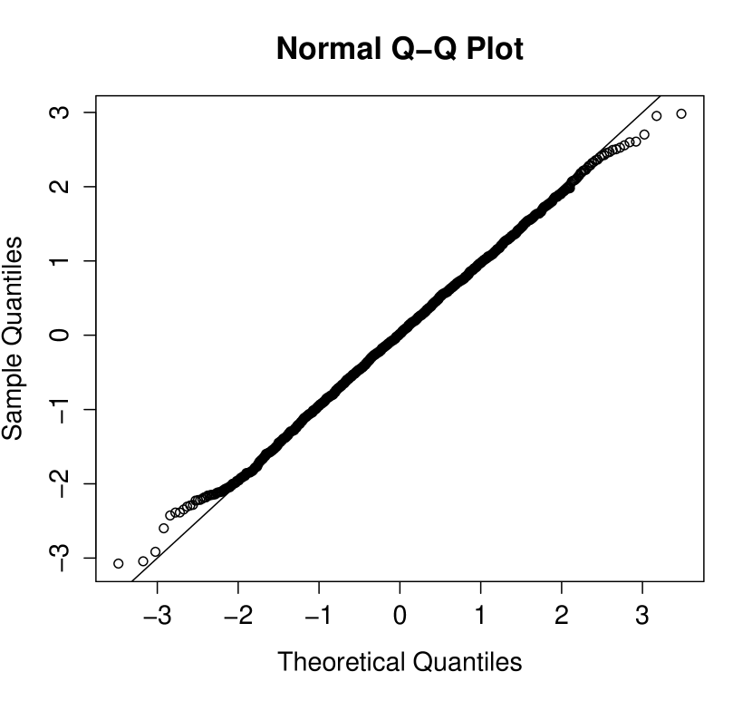
4. Illustrative simulations
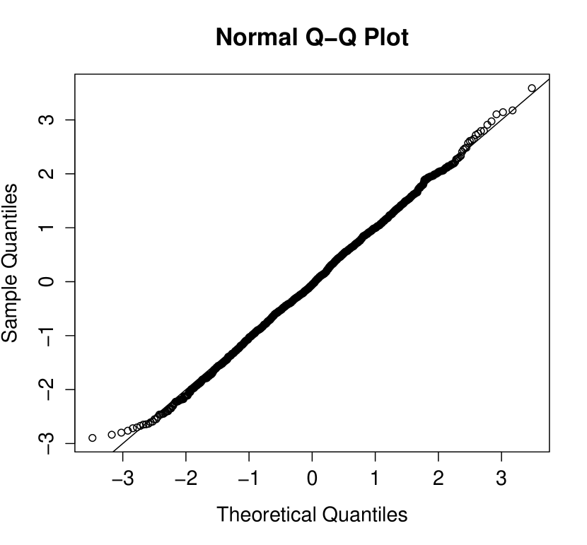
We now turn to a numerical illustration of the theoretical convergence results given in Section 3.2. We are looking at simulations of CARMA processes and their numerically approximated truncated Fourier transform over different time horizons and maximal grid widths. To illustrate the convergence to the asymptotic normal distribution we shall look at several frequencies and different driving Lévy processes, standard Brownian motion, a Variance Gamma process and a “two sided Poisson process”. Of course, the truncated Fourier transform of (Yt)subscript𝑌𝑡(Y_{t}) is obtained using the trapezoidal rule based on non-equidistant observations of the CARMA process (Yt)subscript𝑌𝑡(Y_{t}) given on the interval [0,T]0𝑇[0,T]. On an interval [0,T]0𝑇[0,T] we generate a non-equidistant grid in the following way: we fix the maximal distance hmax(T)subscript𝑇h_{\max}(T) between elements of the grid and from each interval [i12hmax(T),(i+1)12hmax(T))𝑖12subscript𝑇𝑖112subscript𝑇\left[i\cdot\frac{1}{2}h_{\max}(T),(i+1)\cdot\frac{1}{2}h_{\max}(T)\right) for i=0,1,,N1𝑖01𝑁1i=0,1,\dots,N-1 we draw a number according to the uniform distribution. This results in a non-equidistant grid with the number of points being N(T)=2T/hmax+1𝑁𝑇2𝑇subscript1N(T)=2T/h_{\max}+1.
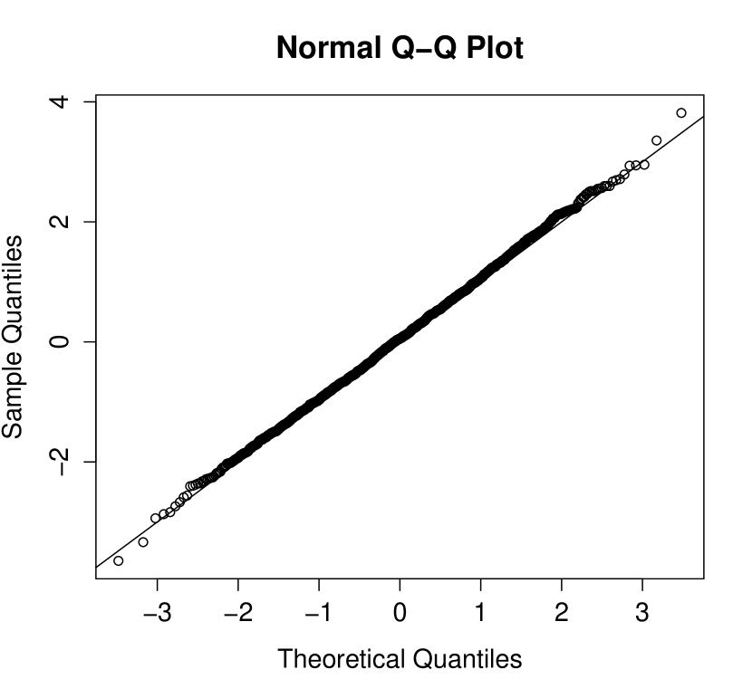
For our simulations we used the R Project for Statistical Computing. For the simulation we first generate the non-equidistant grid by the above procedure and then join it with a regular grid of mesh 0.001, which is still on average five times finer than the non-equidistant grid of the largest time horizon considered. On this joint grid the CARMA process Y𝑌Y is simulated with a standard Euler scheme for the state space representation. Afterwards only the simulated values at the times of the original non-equidistant grid are used to compute the approximation of the truncated Fourier transform with the trapezoidal rule. In all cases we simulate 2000 independent paths of the CARMA process and compute the associated values of the truncated Fourier transform at the following frequencies:

[ω1,ω2,ω3,ω4]=[0, 0.1, 1, 10].subscript𝜔1subscript𝜔2subscript𝜔3subscript𝜔400.1110[\omega_{1},\omega_{2},\omega_{3},\omega_{4}]=[0,\,0.1,\,1,\,10].

For the non-zero frequencies real and imaginary part have to be considered separately. However, in the following we look only at the real parts as the behaviour of the imaginary parts is most similar. Mainly, the results are presented via QQ-plots where the theoretical values follow the (limiting) law described in Theorem 3.15.

We are going to consider CARMA processes with the following autoregressive and moving average orders: (p,q)=(1,0)𝑝𝑞10(p,q)=(1,0), i.e. an Ornstein-Uhlenbeck type process, and (p,q)=(2,1)𝑝𝑞21(p,q)=(2,1). For the time horizon T𝑇T and the maximum distance of the non-equidistant observation times we consider the pairs (T=10,hmax=0.1)formulae-sequence𝑇10subscript0.1(T=10,\,h_{\max}=0.1), (T=50,hmax=0.05)formulae-sequence𝑇50subscript0.05(T=50,\,h_{\max}=0.05) and (T=100,hmax=0.01)formulae-sequence𝑇100subscript0.01(T=100,\,h_{\max}=0.01).

For each case we consider three different driving Lévy noises: standard Brownian Motion, a Variance Gamma process and a “two sided Poisson process”. For the definition and properties of the Variance Gamma process we refer to [MadanCarrChang1998] and references therein. We construct the process in the following way: Vt=Gt1Gt2subscript𝑉𝑡superscriptsubscript𝐺𝑡1superscriptsubscript𝐺𝑡2V_{t}=G_{t}^{1}-G_{t}^{2}, where Gt1superscriptsubscript𝐺𝑡1G_{t}^{1} and Gt2superscriptsubscript𝐺𝑡2G_{t}^{2} are independent Gamma processes with shape parameter 111 and scale parameter 444. Likewise the “two sided Poisson process” is the difference of two independent Poisson processes with rate 101010, i.e. a compound Poisson process with rate 202020 and jumps +11+1 and 11-1 both with probability 1/2121/2.
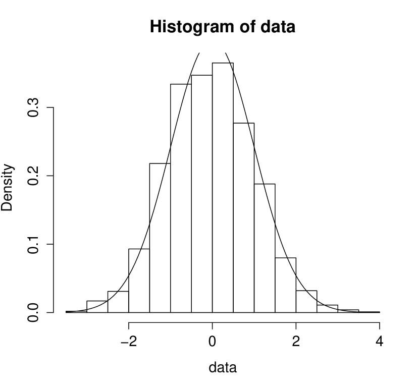
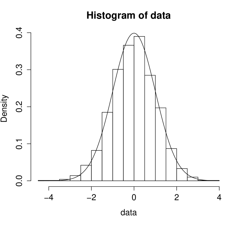
Example 4.1.

We consider the CAR(1)CAR1\operatorname{CAR}(1) model. Then 𝐀=a1𝐀subscript𝑎1\mathbf{A}=-a_{1} and

a(z):=z+a1,b(z)=b0.formulae-sequenceassign𝑎𝑧𝑧subscript𝑎1𝑏𝑧subscript𝑏0a(z):=z+a_{1},\quad b(z)=b_{0}.

So the spectral density is

f(ω)=σ22π|b(iω)a(iω)|2=σ22πb02ω2+a12.𝑓𝜔superscript𝜎22𝜋superscript𝑏𝑖𝜔𝑎𝑖𝜔2superscript𝜎22𝜋superscriptsubscript𝑏02superscript𝜔2superscriptsubscript𝑎12f(\omega)=\frac{\sigma^{2}}{2\pi}\left|\frac{b(i\omega)}{a(i\omega)}\right|^{2}=\frac{\sigma^{2}}{2\pi}\frac{b_{0}^{2}}{\omega^{2}+a_{1}^{2}}.

For the simulations we take [b0,a1]=[1,2]subscript𝑏0subscript𝑎112[b_{0},a_{1}]=[1,2].

QQ-plots showing the results for 2000 simulated paths for the four different frequencies and three different combinations of time horizon and maximum grid width can be found in Figures 1, 2 and 3 for the driving Lévy process being a standard Brownian motion, a Variance Gamma and a two-sided Poisson process, respectively.

Example 4.2.

We consider the CARMA(2,1)CARMA21\operatorname{CARMA}(2,1) model. We have

𝐀:=[01a2a1],𝐛:=[b01],𝐞:=[01],𝐗t:=[X(t)X(1)(t)]formulae-sequenceassign𝐀delimited-[]matrix01subscript𝑎2subscript𝑎1formulae-sequenceassign𝐛delimited-[]matrixsubscript𝑏01formulae-sequenceassign𝐞delimited-[]matrix01assignsubscript𝐗𝑡delimited-[]matrix𝑋𝑡superscript𝑋1𝑡\mathbf{A}:=\left[\begin{matrix}0&1\\ -a_{2}&-a_{1}\\ \end{matrix}\right],\quad\mathbf{b}:=\left[\begin{matrix}b_{0}\\ 1\\ \end{matrix}\right],\quad\mathbf{e}:=\left[\begin{matrix}0\\ 1\\ \end{matrix}\right],\quad\mathbf{X}_{t}:=\left[\begin{matrix}X(t)\\ X^{(1)}(t)\\ \end{matrix}\right]

The autoregressive and moving-average polynomials are of the form

a(z)=z2+a1z+a2,b(z)=z+b0.formulae-sequence𝑎𝑧superscript𝑧2subscript𝑎1𝑧subscript𝑎2𝑏𝑧𝑧subscript𝑏0a(z)=z^{2}+a_{1}z+a_{2},\quad b(z)=z+b_{0}.

We have

b(iω)a(iω)=iω+b0(iω)2+(iω)a1+a2,f(ω)=σ22π|b(iω)a(iω)|2=σ22πb02+ω2ω4+(a122a2)ω2+a22formulae-sequence𝑏𝑖𝜔𝑎𝑖𝜔𝑖𝜔subscript𝑏0superscript𝑖𝜔2𝑖𝜔subscript𝑎1subscript𝑎2𝑓𝜔superscript𝜎22𝜋superscript𝑏𝑖𝜔𝑎𝑖𝜔2superscript𝜎22𝜋superscriptsubscript𝑏02superscript𝜔2superscript𝜔4superscriptsubscript𝑎122subscript𝑎2superscript𝜔2superscriptsubscript𝑎22\frac{b(i\omega)}{a(i\omega)}=\frac{i\omega+b_{0}}{(i\omega)^{2}+(i\omega)a_{1}+a_{2}},\quad f(\omega)=\frac{\sigma^{2}}{2\pi}\left|\frac{b(i\omega)}{a(i\omega)}\right|^{2}=\frac{\sigma^{2}}{2\pi}\frac{b_{0}^{2}+\omega^{2}}{\omega^{4}+(a_{1}^{2}-2a_{2})\omega^{2}+a_{2}^{2}}

For the simulation procedure we take [b0,b1,a1,a2]=[1,1,1,2]subscript𝑏0subscript𝑏1subscript𝑎1subscript𝑎21112[b_{0},b_{1},a_{1},a_{2}]=[1,1,1,2].

QQ-plots showing the results for 2000 simulated paths for the four different frequencies and three different combinations of time horizon and maximum grid width can be found in Figures 4, 6 and 8 for the driving Lévy process being a standard Brownian motion, a Variance Gamma and a two-sided Poisson process, respectively. Likewise, Figures 5, 7 and 9 show corresponding histograms.

Refer to caption
(a) ω=0,T=10formulae-sequence𝜔0𝑇10\omega=0,T=10
Refer to caption
(b) ω=0,T=50formulae-sequence𝜔0𝑇50\omega=0,T=50
Refer to caption
(c) ω=0,T=100formulae-sequence𝜔0𝑇100\omega=0,T=100
Refer to caption
(d) ω=0.1,T=10formulae-sequence𝜔0.1𝑇10\omega=0.1,T=10
Refer to caption
(e) ω=0.1,T=50formulae-sequence𝜔0.1𝑇50\omega=0.1,T=50
Refer to caption
(f) ω=0.1,T=100formulae-sequence𝜔0.1𝑇100\omega=0.1,T=100
Refer to caption
(g) ω=1,T=10formulae-sequence𝜔1𝑇10\omega=1,T=10
Refer to caption
(h) ω=1,T=50formulae-sequence𝜔1𝑇50\omega=1,T=50
Refer to caption
(i) ω=1,T=100formulae-sequence𝜔1𝑇100\omega=1,T=100
Refer to caption
(j) ω=10,T=10formulae-sequence𝜔10𝑇10\omega=10,T=10
Refer to caption
(k) ω=10,T=50formulae-sequence𝜔10𝑇50\omega=10,T=50
Refer to caption
(l) ω=10,T=100formulae-sequence𝜔10𝑇100\omega=10,T=100
Figure 1. Normal QQ plots for the real part of the truncated Fourier transform of the Ornstein-Uhlenbeck type process driven by standard Brownian Motion for the frequencies 0,0.1,1,1000.11100,0.1,1,10 (rows) and time horizons/maximum non-equidistant grid sizes 10/0.1,50/0.05,100/0.01100.1500.051000.0110/0.1,50/0.05,100/0.01 (columns). The theoretical quantiles are coming from the (limiting) law described in Theorem 3.15.
Refer to caption
(a) ω=0,T=10formulae-sequence𝜔0𝑇10\omega=0,T=10
Refer to caption
(b) ω=0,T=50formulae-sequence𝜔0𝑇50\omega=0,T=50
Refer to caption
(c) ω=0,T=100formulae-sequence𝜔0𝑇100\omega=0,T=100
Refer to caption
(d) ω=0.1,T=10formulae-sequence𝜔0.1𝑇10\omega=0.1,T=10
Refer to caption
(e) ω=0.1,T=50formulae-sequence𝜔0.1𝑇50\omega=0.1,T=50
Refer to caption
(f) ω=0.1,T=100formulae-sequence𝜔0.1𝑇100\omega=0.1,T=100
Refer to caption
(g) ω=1,T=10formulae-sequence𝜔1𝑇10\omega=1,T=10
Refer to caption
(h) ω=1,T=50formulae-sequence𝜔1𝑇50\omega=1,T=50
Refer to caption
(i) ω=1,T=100formulae-sequence𝜔1𝑇100\omega=1,T=100
Refer to caption
(j) ω=10,T=10formulae-sequence𝜔10𝑇10\omega=10,T=10
Refer to caption
(k) ω=10,T=50formulae-sequence𝜔10𝑇50\omega=10,T=50
Refer to caption
(l) ω=10,T=100formulae-sequence𝜔10𝑇100\omega=10,T=100
Figure 2. Normal QQ plots for the real part of the truncated Fourier transform of the Ornstein-Uhlenbeck type process driven by a Variance Gamma process for the frequencies 0,0.1,1,1000.11100,0.1,1,10 (rows) and time horizons/maximum non-equidistant grid sizes 10/0.1,50/0.05,100/0.01100.1500.051000.0110/0.1,50/0.05,100/0.01 (columns). The theoretical quantiles are coming from the (limiting) law described in Theorem 3.15.
Refer to caption
(a) ω=0,T=10formulae-sequence𝜔0𝑇10\omega=0,T=10
Refer to caption
(b) ω=0,T=50formulae-sequence𝜔0𝑇50\omega=0,T=50
Refer to caption
(c) ω=0,T=100formulae-sequence𝜔0𝑇100\omega=0,T=100
Refer to caption
(d) ω=0.1,T=10formulae-sequence𝜔0.1𝑇10\omega=0.1,T=10
Refer to caption
(e) ω=0.1,T=50formulae-sequence𝜔0.1𝑇50\omega=0.1,T=50
Refer to caption
(f) ω=0.1,T=100formulae-sequence𝜔0.1𝑇100\omega=0.1,T=100
Refer to caption
(g) ω=1,T=10formulae-sequence𝜔1𝑇10\omega=1,T=10
Refer to caption
(h) ω=1,T=50formulae-sequence𝜔1𝑇50\omega=1,T=50
Refer to caption
(i) ω=1,T=100formulae-sequence𝜔1𝑇100\omega=1,T=100
Refer to caption
(j) ω=10,T=10formulae-sequence𝜔10𝑇10\omega=10,T=10
Refer to caption
(k) ω=10,T=50formulae-sequence𝜔10𝑇50\omega=10,T=50
Refer to caption
(l) ω=10,T=100formulae-sequence𝜔10𝑇100\omega=10,T=100
Figure 3. Normal QQ plots for the real part of the truncated Fourier transform of the Ornstein-Uhlenbeck type process driven by a two-sided Poisson process for the frequencies 0,0.1,1,1000.11100,0.1,1,10 (rows) and time horizons/maximum non-equidistant grid sizes 10/0.1,50/0.05,100/0.01100.1500.051000.0110/0.1,50/0.05,100/0.01 (columns). The theoretical quantiles are coming from the (limiting) law described in Theorem 3.15.
Refer to caption
(a) ω=0,T=10formulae-sequence𝜔0𝑇10\omega=0,T=10
Refer to caption
(b) ω=0,T=50formulae-sequence𝜔0𝑇50\omega=0,T=50
Refer to caption
(c) ω=0,T=100formulae-sequence𝜔0𝑇100\omega=0,T=100
Refer to caption
(d) ω=0.1,T=10formulae-sequence𝜔0.1𝑇10\omega=0.1,T=10
Refer to caption
(e) ω=0.1,T=50formulae-sequence𝜔0.1𝑇50\omega=0.1,T=50
Refer to caption
(f) ω=0.1,T=100formulae-sequence𝜔0.1𝑇100\omega=0.1,T=100
Refer to caption
(g) ω=1,T=10formulae-sequence𝜔1𝑇10\omega=1,T=10
Refer to caption
(h) ω=1,T=50formulae-sequence𝜔1𝑇50\omega=1,T=50
Refer to caption
(i) ω=1,T=100formulae-sequence𝜔1𝑇100\omega=1,T=100
Refer to caption
(j) ω=10,T=10formulae-sequence𝜔10𝑇10\omega=10,T=10
Refer to caption
(k) ω=10,T=50formulae-sequence𝜔10𝑇50\omega=10,T=50
Refer to caption
(l) ω=10,T=100formulae-sequence𝜔10𝑇100\omega=10,T=100
Figure 4. Normal QQ plots for the real part of the truncated Fourier transform of the simulated CARMA(2,1) processes driven by standard Brownian Motion for the frequencies 0,0.1,1,1000.11100,0.1,1,10 (rows) and time horizons/maximum non-equidistant grid sizes 10/0.1,50/0.05,100/0.01100.1500.051000.0110/0.1,50/0.05,100/0.01 (columns). The theoretical quantiles are coming from the (limiting) law described in Theorem 3.15.
Refer to caption
(a) ω=0,T=10formulae-sequence𝜔0𝑇10\omega=0,T=10
Refer to caption
(b) ω=0,T=50formulae-sequence𝜔0𝑇50\omega=0,T=50
Refer to caption
(c) ω=0,T=100formulae-sequence𝜔0𝑇100\omega=0,T=100
Refer to caption
(d) ω=0.1,T=10formulae-sequence𝜔0.1𝑇10\omega=0.1,T=10
Refer to caption
(e) ω=0.1,T=50formulae-sequence𝜔0.1𝑇50\omega=0.1,T=50
Refer to caption
(f) ω=0.1,T=100formulae-sequence𝜔0.1𝑇100\omega=0.1,T=100
Refer to caption
(g) ω=1,T=10formulae-sequence𝜔1𝑇10\omega=1,T=10
Refer to caption
(h) ω=1,T=50formulae-sequence𝜔1𝑇50\omega=1,T=50
Refer to caption
(i) ω=1,T=100formulae-sequence𝜔1𝑇100\omega=1,T=100
Refer to caption
(j) ω=10,T=10formulae-sequence𝜔10𝑇10\omega=10,T=10
Refer to caption
(k) ω=10,T=50formulae-sequence𝜔10𝑇50\omega=10,T=50
Refer to caption
(l) ω=10,T=100formulae-sequence𝜔10𝑇100\omega=10,T=100
Figure 5. Histograms and limiting density for the real part of the truncated Fourier transform of the simulated CARMA(2,1) processes driven by standard Brownian Motion for the frequencies 0,0.1,1,1000.11100,0.1,1,10 (rows) and time horizons/maximum non-equidistant grid sizes 10/0.1,50/0.05,100/0.01100.1500.051000.0110/0.1,50/0.05,100/0.01 (columns)
Refer to caption
(a) ω=0,T=10formulae-sequence𝜔0𝑇10\omega=0,T=10
Refer to caption
(b) ω=0,T=50formulae-sequence𝜔0𝑇50\omega=0,T=50
Refer to caption
(c) ω=0,T=100formulae-sequence𝜔0𝑇100\omega=0,T=100
Refer to caption
(d) ω=0.1,T=10formulae-sequence𝜔0.1𝑇10\omega=0.1,T=10
Refer to caption
(e) ω=0.1,T=50formulae-sequence𝜔0.1𝑇50\omega=0.1,T=50
Refer to caption
(f) ω=0.1,T=100formulae-sequence𝜔0.1𝑇100\omega=0.1,T=100
Refer to caption
(g) ω=1,T=10formulae-sequence𝜔1𝑇10\omega=1,T=10
Refer to caption
(h) ω=1,T=50formulae-sequence𝜔1𝑇50\omega=1,T=50
Refer to caption
(i) ω=1,T=100formulae-sequence𝜔1𝑇100\omega=1,T=100
Refer to caption
(j) ω=10,T=10formulae-sequence𝜔10𝑇10\omega=10,T=10
Refer to caption
(k) ω=10,T=50formulae-sequence𝜔10𝑇50\omega=10,T=50
Refer to caption
(l) ω=10,T=100formulae-sequence𝜔10𝑇100\omega=10,T=100
Figure 6. Normal QQ plots for the real part of the truncated Fourier transform of the simulated CARMA(2,1) processes driven by a Variance Gamma process for the frequencies 0,0.1,1,1000.11100,0.1,1,10 (rows) and time horizons/maximum non-equidistant grid sizes 10/0.1,50/0.05,100/0.01100.1500.051000.0110/0.1,50/0.05,100/0.01 (columns). The theoretical quantiles are coming from the (limiting) law described in Theorem 3.15.
Refer to caption
(a) ω=0,T=10formulae-sequence𝜔0𝑇10\omega=0,T=10
Refer to caption
(b) ω=0,T=50formulae-sequence𝜔0𝑇50\omega=0,T=50
Refer to caption
(c) ω=0,T=100formulae-sequence𝜔0𝑇100\omega=0,T=100
Refer to caption
(d) ω=0.1,T=10formulae-sequence𝜔0.1𝑇10\omega=0.1,T=10
Refer to caption
(e) ω=0.1,T=50formulae-sequence𝜔0.1𝑇50\omega=0.1,T=50
Refer to caption
(f) ω=0.1,T=100formulae-sequence𝜔0.1𝑇100\omega=0.1,T=100
Refer to caption
(g) ω=1,T=10formulae-sequence𝜔1𝑇10\omega=1,T=10
Refer to caption
(h) ω=1,T=50formulae-sequence𝜔1𝑇50\omega=1,T=50
Refer to caption
(i) ω=1,T=100formulae-sequence𝜔1𝑇100\omega=1,T=100
Refer to caption
(j) ω=10,T=10formulae-sequence𝜔10𝑇10\omega=10,T=10
Refer to caption
(k) ω=10,T=50formulae-sequence𝜔10𝑇50\omega=10,T=50
Refer to caption
(l) ω=10,T=100formulae-sequence𝜔10𝑇100\omega=10,T=100
Figure 7. Histograms and limiting density for the real part of the truncated Fourier transform of the simulated CARMA(2,1) processes driven by a Variance Gamma process for the frequencies 0,0.1,1,1000.11100,0.1,1,10 (rows) and time horizons/maximum non-equidistant grid sizes 10/0.1,50/0.05,100/0.01100.1500.051000.0110/0.1,50/0.05,100/0.01 (columns)
Refer to caption
(a) ω=0,T=10formulae-sequence𝜔0𝑇10\omega=0,T=10
Refer to caption
(b) ω=0,T=50formulae-sequence𝜔0𝑇50\omega=0,T=50
Refer to caption
(c) ω=0,T=100formulae-sequence𝜔0𝑇100\omega=0,T=100
Refer to caption
(d) ω=0.1,T=10formulae-sequence𝜔0.1𝑇10\omega=0.1,T=10
Refer to caption
(e) ω=0.1,T=50formulae-sequence𝜔0.1𝑇50\omega=0.1,T=50
Refer to caption
(f) ω=0.1,T=100formulae-sequence𝜔0.1𝑇100\omega=0.1,T=100
Refer to caption
(g) ω=1,T=10formulae-sequence𝜔1𝑇10\omega=1,T=10
Refer to caption
(h) ω=1,T=50formulae-sequence𝜔1𝑇50\omega=1,T=50
Refer to caption
(i) ω=1,T=100formulae-sequence𝜔1𝑇100\omega=1,T=100
Refer to caption
(j) ω=10,T=10formulae-sequence𝜔10𝑇10\omega=10,T=10
Refer to caption
(k) ω=10,T=50formulae-sequence𝜔10𝑇50\omega=10,T=50
Refer to caption
(l) ω=10,T=100formulae-sequence𝜔10𝑇100\omega=10,T=100
Figure 8. Normal QQ plots for the real part of the truncated Fourier transform of the simulated CARMA(2,1) processes driven by a two sided Poisson process for the frequencies 0,0.1,1,1000.11100,0.1,1,10 (rows) and time horizons/maximum non-equidistant grid sizes 10/0.1,50/0.05,100/0.01100.1500.051000.0110/0.1,50/0.05,100/0.01 (columns). The theoretical quantiles are coming from the (limiting) law described in Theorem 3.15.
Refer to caption
(a) ω=0,T=10formulae-sequence𝜔0𝑇10\omega=0,T=10
Refer to caption
(b) ω=0,T=50formulae-sequence𝜔0𝑇50\omega=0,T=50
Refer to caption
(c) ω=0,T=100formulae-sequence𝜔0𝑇100\omega=0,T=100
Refer to caption
(d) ω=0.1,T=10formulae-sequence𝜔0.1𝑇10\omega=0.1,T=10
Refer to caption
(e) ω=0.1,T=50formulae-sequence𝜔0.1𝑇50\omega=0.1,T=50
Refer to caption
(f) ω=0.1,T=100formulae-sequence𝜔0.1𝑇100\omega=0.1,T=100
Refer to caption
(g) ω=1,T=10formulae-sequence𝜔1𝑇10\omega=1,T=10
Refer to caption
(h) ω=1,T=50formulae-sequence𝜔1𝑇50\omega=1,T=50
Refer to caption
(i) ω=1,T=100formulae-sequence𝜔1𝑇100\omega=1,T=100
Refer to caption
(j) ω=10,T=10formulae-sequence𝜔10𝑇10\omega=10,T=10
Refer to caption
(k) ω=10,T=50formulae-sequence𝜔10𝑇50\omega=10,T=50
Refer to caption
(l) ω=10,T=100formulae-sequence𝜔10𝑇100\omega=10,T=100
Figure 9. Histograms and limiting density for the real part of the truncated Fourier transform of the simulated CARMA(2,1) processes driven by a two-sided Poisson process for the frequencies 0,0.1,1,1000.11100,0.1,1,10 (rows) and time horizons/maximum non-equidistant grid sizes 10/0.1,50/0.05,100/0.01100.1500.051000.0110/0.1,50/0.05,100/0.01 (columns)

The simulation results seem to indicate the following.

In Figure 1 we notice at first a pretty good fit of the empirical quantiles from the simulations with the theoretical ones of the asymptotic distribution across all time horizons and frequencies. Looking more carefully, the fit in the tails clearly improves when the time horizon/fineness of the grid increases, but it is never bad. For the longest time horizon and finest grid the fit is clearly very good. Of course, it should not be forgotten that in this case the distribution of the (trapezoidal approximation of the) truncated Fourier transform is always exactly Gaussian and not only asymptotically. When looking across the non-zero frequencies one notes that for the shortest time horizon the quantiles for the smallest frequency 0.10.10.1 appear to lie on a line which is somewhat different from the line of the theoretical quantiles. This indicates that the quantiles of the simulated paths come from a normal distribution, but one with a different variance then the asymptotic one. It is no surprise that this occurs for the lowest frequency and the smallest time interval, as for low frequencies one observes – regardless of the fineness of the sampling – the fewest full cycles over a time interval of fixed length. For this combination of time horizon and frequency we see only one full cycle.

Turning to Figure 2, we first notice that the fit in the tails improves again clearly with increasing (T,1/hmax)𝑇1subscript(T,1/h_{\max}). Especially, for the highest (T,1/hmax)𝑇1subscript(T,1/h_{\max}) one sees that the fit in the tails is a bit worse now for a driving Variance Gamma process compared with the driving Brownian motion in Figure 1. Of course, now the simulated values are indeed only asymptotically following a Gaussian distribution. Looking at the different non-zero frequencies one again sees that the fit improves for the higher frequencies. Most notably for the lowest frequency one sees for the smallest T=10𝑇10T=10 again that the points do seem to lie on a straight line in the normal QQ-plot, but one with a different slope than for the theoretical quantiles. Hence, the variance is clearly different from the asmpytotic one. Obviously, this effect is now more pronounced than in the case of the driving Brownian motion.

Moving on to the case of the driving process being a two-sided Poisson process in Figure 3 we first of all note that again the fit in particular in the tails clearly improves with increasing (T,1/hmax)𝑇1subscript(T,1/h_{\max}). For the highest (T,1/hmax)𝑇1subscript(T,1/h_{\max}) the simulated and theoretical asymptotic quantiles agree again extremely well. Again it is certainly a bit worse than in the case of a driving Brownian motion, but it seems to be very similar to the Variance Gamma case, although maybe for frequency 00 the agreement of the quantiles is slightly worse. Turning to the behaviour across non-zero frequencies, we see again that the quantiles are closer for higher frequencies and that for the smallest non-zero frequency and time horizon the empirical quantiles seem to be in line with a normal distribution with a somewhat different variance compared to the asymptotic one. The size of this effect seems to be rather similar to the Variance Gamma case. Interestingly, also at frequency 00 the QQ-plot seems to indicate for T=10𝑇10T=10 that the empirical quantiles are close to the ones of a normal distribution with a slightly different variance than the asymptotic one.

To summarize the simulation study in the CAR(1)/OU-type case we can clearly conclude that the asymptotic distribution result approximates the finite-sample distribution of the trapezoidal approximation of the truncated Fourier transform in our simulations very well and that the convergence to the asymptotic distribution is fast. For small frequencies, especially when one has about one full cycle or less over the time horizon considered, one has to be careful, as then the distribution tends to be somewhat different from the asymptotic one for good reasons. This effect seems to be more pronounced when one considers a Lévy process with jumps compared to a Brownian motion. In general the quality of the approximation of the simulated quantiles by the asymptotic ones is somewhat better in the case of a Brownian motion than in a pure jump process. Comparing the driving jump processes, the finite activity rather discrete two-sided Poisson process with the infinite activity Variance Gamma process, we do not see any significant differences. It should be noted that both jump processes are, however, light-tailed in the sense that they have exponential moments. It would not be surprising if this picture changes when considering a really heavily tailed driving Lévy process. Note that our theoretical results are valid also in rather heavily-tailed cases. For the asymptotic normality of the (trapezoidal approximation of the) truncated Fourier transform we only needed finite second moments.

Turning to the simulations of CARMA(2,1) processes, most of the findings of the CAR(1)/OU case remain valid, so we only point out the differences. In the case of a driving Brownian motion, depicted in Figure 4, the only difference seems to be that for T=10𝑇10T=10 and ω=0.1𝜔0.1\omega=0.1 the empirical quantiles are now appearing to lie on a line farther away from the theoretical quantiles which implies that in the CARMA(2,1) case the variance in the simulations is clearly farther away from the asymptotic one than in the OU case. The same applies for the Variance Gamma case of Figure 6 and the two-sided Poisson case of Figure 6. On top of the QQ plots we now also provide histograms in Figures 5, 7 and 9, respectively, together with plots of the limiting normal density. To us it seems very hard to see the convergence to normality with increasing T𝑇T in the histograms, which reflects the fact that it is essentially the tails which need to converge and they are much clearer visible in the QQ plots than in histograms. It is also not easy to see in them that for ω=0.1,T=10formulae-sequence𝜔0.1𝑇10\omega=0.1,\,T=10 the variance of the simulated values is different from the asymptotic theoretical one. The only thing one notices is that for ω=0.1,T=10formulae-sequence𝜔0.1𝑇10\omega=0.1,\,T=10 the histogram routine of R tends to use very different bins than in all the other cases. Note that all histograms were obtained using the default parameters of the hist function in R, so the binning was done by the standard automatic selection to give “nice” histograms. Hence, from our simulations of CARMA(2,1) processes we can conclude that the orders of the CARMA processes and the particular autoregressive and moving average parameters appear not to really matter for the (qualitative) behaviour of the (trapezoidal approximation of the) truncated Fourier transform.

5. Conclusion and Outlook

We have obtained an asymptotic normality result for the (trapezoidal approximation of the) truncated Fourier transform under essentially minimal assumptions (i.e. second moments) and seen via a simulation study that this result approximates the finite sample behaviour very well, unless the frequency is too low compared to the length of the considered time interval. This suggests clearly that it should be very promising to develop statistical inference techniques for non-equidistantly sampled CARMA processes by considering continuous observation techniques and using numerical approximation schemes to compute the quantities of interest based on the observed non-equidistant data. The appropriate set-up to get convergence and asymptotic distribution results is to send the time horizon to infinity and to send at the same time the maximum distance of observation time points to zero.

Based on our results in this paper it seems natural to locally smooth the trapezoidal approximation of the truncated Fourier transform to get consistent estimators of the spectral density and to use it in a Whittle type estimator for the AR and MA parameters. Considering this is beyond the scope of the present paper.

Acknowledgements

The authors gratefully acknowledge the support of Deutsche Forschungsgemeinschaft (DFG) by research grant STE 2005/1-2.

The authors would like to cordially thank Włodzimierz Fechner for careful reading of the manuscript and his helpful remarks.

References

    @book{Applebaum2009}
  • AUTHOR = Applebaum, David, TITLE = Lévy processes and stochastic calculus, EDITION = Second Edition, PUBLISHER = Cambridge University Press, Cambridge, YEAR = 2009, PAGES = xxx+460,
  • BillingsleyPatrickProbability and measureWiley Series in Probability and Mathematical StatisticsThirdJohn Wiley & Sons, Inc., New York1995xiv+593ISBN 0-471-00710-2@book{Billingsley1995, author = {Billingsley, Patrick}, title = {Probability and measure}, series = {Wiley Series in Probability and Mathematical Statistics}, edition = {Third}, publisher = {John Wiley \& Sons, Inc., New York}, year = {1995}, pages = {xiv+593}, isbn = {0-471-00710-2}} BrockwellPeter J.Lévy-driven carma processesAnn. Inst. Statist. Math.53200196-120113––124@article{Brockwell2001, author = {Brockwell, Peter J.}, title = {Lévy-driven CARMA processes}, journal = {Ann. Inst. Statist. Math.}, volume = {53}, date = {2001}, number = {96-120}, pages = {113–-124}} BrockwellPeter J.Continuous-time ARMA processesStochastic processes: theory and methodsin: Handbook of Statistics, Eds.: D.N. Shanbhag, C.R. Rao19249–276North-Holland, Amsterdam2001@book{Brockwell2001a, author = {Brockwell, Peter J.}, title = {Continuous-time {ARMA} processes}, booktitle = {Stochastic processes: theory and methods}, series = {in: Handbook of Statistics, Eds.: D.N. Shanbhag, C.R. Rao}, volume = {19}, pages = {249–276}, publisher = {North-Holland, Amsterdam}, year = {2001}} BrockwellPeter J.Representations of continuous-time arma processesJ. Appl. Probab41A2004375–382@article{Brockwell2004, author = {Brockwell, Peter J.}, title = {Representations of continuous-time ARMA processes}, journal = {J. Appl. Probab}, volume = {41A}, date = {2004}, pages = {375–382}} BrockwellPeter J.Lévy driven continuous-time arma processesin: Handbook of financial time series, Eds.: T.G. Andersen, R.A. Davis, J.-P. Kreiss and T. MikoschHandbook of financial time seriesHeidelberg: Springer2009653–67@book{Brockwell2009, author = {Brockwell, Peter J.}, title = {L\'evy driven continuous-time ARMA processes}, series = {in: Handbook of financial time series, Eds.: T.G. Andersen, R.A. Davis, J.-P. Kreiss and T. Mikosch}, booktitle = {Handbook of financial time series}, publisher = {Heidelberg: Springer}, year = {2009}, pages = {653–67}} BrockwellPeter J.DavisRichard A.Time series: theory and methodsReprint of the 2nd (1991) editionSpringer, New York2006xvi+577@book{BrockwellDavis, author = {Brockwell, Peter J.}, author = {Davis, Richard A.}, title = {Time series: theory and methods}, note = {Reprint of the 2nd (1991) edition}, publisher = {Springer, New York}, year = {2006}, pages = {xvi+577}} BrockwellPeter J.DavisRichard A.YangYuEstimation for non-negative Lévy-driven CARMA processesJ. Bus. Econom. Statist.2920112250–259@article{BrockwellDavisYang, author = {Brockwell, Peter J. and Davis, Richard A. and Yang, Yu}, title = {Estimation for non-negative {L}\'evy-driven {CARMA} processes}, journal = {J. Bus. Econom. Statist.}, volume = {29}, year = {2011}, number = {2}, pages = {250–259}} BrockwellPeter J.LindnerAlexanderExistence and uniqueness of stationary lévy-driven carma processesStochastic Process. Appl.119200982660–2681@article{BrockwellLindner2009, author = {Brockwell, Peter J.}, author = {Lindner, Alexander}, title = {Existence and uniqueness of stationary L\'evy-driven CARMA processes}, journal = {Stochastic Process. Appl.}, volume = {119}, date = {2009}, number = {8}, pages = {2660–2681}} BrockwellPeter J.SchlemmEckhardParametric estimation of the driving Lévy process of multivariate CARMA processes from discrete observationsJ. Multivariate Anal.1152013217–251@article{BrockwellSchlemm, author = {Brockwell, Peter J.}, author = {Schlemm, Eckhard}, title = {Parametric estimation of the driving {L}\'evy process of multivariate {CARMA} processes from discrete observations}, journal = {J. Multivariate Anal.}, volume = {115}, year = {2013}, pages = {217–251}} @article{Doob}
  • AUTHOR = Doob, J. L., TITLE = The elementary Gaussian processes, JOURNAL = Ann. Math. Statistics, VOLUME = 15, YEAR = 1944, PAGES = 229–282,
  • @article{Fasen2013}
  • year=2013, journal=Math. Methods Statist., volume=22, number=4, title=Statistical inference of spectral estimation for continuous-time MA processes with finite second moments, author=Fasen, V., pages=283-309
  • @article{FuchsFasen2013}
  • AUTHOR = Fasen, Vicky, AUTHOR = Fuchs, Florian, TITLE = Spectral estimates for high-frequency sampled continuous-time autoregressive moving average processes, JOURNAL = J. Time Series Anal., VOLUME = 34, YEAR = 2013, NUMBER = 5, PAGES = 532–551,
  • FasenVickyFuchsFlorianOn the limit behavior of the periodogram of high-frequency sampled stable carma processesStochastic Process. Appl.12320131229–273@article{FuchsFasen2013a, author = {Fasen, Vicky}, author = {Fuchs, Florian}, title = {On the limit behavior of the periodogram of high-frequency sampled stable CARMA processes}, journal = {Stochastic Process. Appl.}, volume = {123}, date = {2013}, number = {1}, pages = {229–273}} GillbergJonasFrequency domain identification of continuous-time systems: reconstruction and robustnessLinköping Studies in Science and Technology. Dissertations20061031ISSN 0345-7524@article{Gillberg2006, author = {Gillberg, Jonas }, title = {Frequency Domain Identification of Continuous-Time Systems: Reconstruction and Robustness}, journal = {Linköping Studies in Science and Technology. Dissertations}, date = {2006}, number = {1031}, issn = {0345-7524}} LiiKeh-ShinMasryEliasModel fitting for continuous-time stationary processes from discrete-time dataJ. Multivariate Anal.411992156–79ISSN 0047-259X@article{LiiMasry1992, author = {Lii, Keh-Shin}, author = {Masry, Elias}, title = {Model fitting for continuous-time stationary processes from discrete-time data}, journal = {J. Multivariate Anal.}, volume = {41}, year = {1992}, number = {1}, pages = {56–79}, issn = {0047-259X}} @article{LiiMasry1994}
  • AUTHOR = Lii, Keh-Shin, AUTHOR = Masry, Elias, TITLE = Spectral estimation of continuous-time stationary processes from random sampling, JOURNAL = Stochastic Process. Appl., VOLUME = 52, YEAR = 1994, NUMBER = 1, PAGES = 39–64, ISSN = 0304-4149,
  • MadanDilip B.CarrPeter P.ChangEric C.The variance gamma process and option pricingEuropean Finance Review2199879–105@article{MadanCarrChang1998, author = {Madan, Dilip B.}, author = {Carr, Peter P.}, author = {Chang, Eric C.}, title = {The Variance Gamma Process and Option Pricing}, journal = {European Finance Review}, volume = {2}, year = {1998}, pages = {79–105}} MarquardtTinaStelzerRobertMultivariate CARMA processesStochastic Process. Appl.1172007196–120@article{MarquardtStelzer2007, author = {Marquardt, Tina}, author = {Stelzer, Robert}, title = {Multivariate {CARMA} processes}, journal = {Stochastic Process. Appl.}, volume = {117}, year = {2007}, number = {1}, pages = {96–120}} @book{Protter}
  • AUTHOR = Protter, Philip E., TITLE = Stochastic integration and differential equations, EDITION = 2nd edn., PUBLISHER = Springer-Verlag, Berlin, YEAR = 2004, PAGES = xiv+415, ISBN = 3-540-00313-4,
  • SchlemmEckhardStelzerRobertMultivariate carma processes, continuous-time state space models and complete regularity of the innovations of the sampled processesBernoulli182012146––63@article{SchlemmStelzer2012, author = {Schlemm, Eckhard}, author = {Stelzer, Robert}, title = {Multivariate CARMA processes, continuous-time state space models and complete regularity of the innovations of the sampled processes}, journal = {Bernoulli}, volume = {18}, date = {2012}, number = {1}, pages = {46–-63}} TalvilaErikWiersmaMatthewSimple derivation of basic quadrature formulasAtl. Electron. J. Math.52012147–59@article{TalvilaWiersma2012, author = {Talvila, Erik}, author = {Wiersma, Matthew}, title = {Simple derivation of basic quadrature formulas}, journal = {Atl. Electron. J. Math.}, volume = {5}, year = {2012}, number = {1}, pages = {47–59}} @article{Veraar2012}
  • AUTHOR = Veraar, Mark, TITLE = The stochastic Fubini theorem revisited, JOURNAL = Stochastics, VOLUME = 84, YEAR = 2012, NUMBER = 4, PAGES = 543–551,