Black Holes and Thunderbolt Singularities with Lifshitz Scaling Terms

Abstract

We study a static, spherically symmetric and asymptotic flat spacetime, assuming the hypersurface orthogonal Einstein-aether theory with an ultraviolet modification motivated by the Hořava-Lifshitz theory, which is composed of the $z=2$ Lifshitz scaling terms such as scalar combinations of a three-Ricci curvature and the acceleration of the aether field. For the case with the quartic term of the acceleration of the aether field, we obtain a two-parameter family of black hole solutions, which possess a regular universal horizon. While, if three-Ricci curvature squared term is joined in ultraviolet modification, we find a solution with a thunderbolt singularity such that the universal horizon turns to be a spacelike singularity.

I Introduction

Spacetime singularity is unavoidable in general relativityHawking_Ellis , which means the breakdown of our standard theory of gravity in ultraviolet region. To establish the fundamental gravitational theory beyond general relativity is one of the most intriguing question of physics. One may expect that this difficulty can be resolved by considering the quantum effect of gravity. However, unfortunately, the perturbative quantization approach of general relativity losses the renormalizability unlike the other fundamental interactions. In other words, there appears infinite numbers of divergent Feynman diagrams, and thus, the infinite counter terms are required to regularize the gravitational quantum effects. Hence one way to quantize gravity is non-perturbative approach such as the loop quantum gravityloop or the dynamical triangulationtriangulation .

Another way is to find a new renormalizable gravitational theory. String theory string can be such a candidate, but it has not been completed. Recently, Hořava proposed a gravitational theory with Lifshitz scalingHL_original_paper , which is anisotropic scaling between space and time, i.e., $t\to b^{-1}t\,,~{}x^{i}\to b^{-z}x^{i}$. This scaling defines a scaling dimension $[t]=-z$ with $[x^{i}]=-1$, which is restored to the ordinary mass dimension when $z=1$. It is found that if we set $z$ to the number of the spatial dimension, the dimension of the gravitational constant becomes zero, which means the gravitational force acquires renormalizability at least at a power-counting level. This gravitational theory is called Hořava-Lifshitz (HL) theory whose action includes higher spatial curvature terms up to cubic order as counter terms of renormalization.

Although there is a need for further investigation to confirm whether HL theory is truly renormalizable or notrenormalizability , strong gravitational phenomena, such as cosmological singularity avoidance HL_cosmological_sin_avoicance and the black hole solutionHL_BH_ref have been studied by several authors. In particular, study regarding the spacetime structure is particularly intriguing frontier. Since the spacetime in HL theory losses local Lorentz symmetry due to Lifshitz scaling, the causal structure is drastically changed. If there is Lifshitz scaling with $z\neq 1$, the dispersion relation of the signal particle is modified as $\omega^{2}\sim k^{2z}$, and then the sound speed is given by $c\sim k^{z-1}$. In consequence, the sound speed almost diverges if the particle is in an extremely high energetic state. One may consider it is impossible to define the casual horizon due to such an instantaneously propagating particle. However it is not the case. In the context of the Einstein-aether (æ-) theory EA_original_paper which has some equivalence to the infrared limit of HL theorykhronon_theory , there still exists a causal horizon for such an extreme energetic particle. Although æ-theory itself is a toy model as a Lorentz violating gravitational theory, it is found that the HL theory is reduced to æ-theory in infrared limit if the aether is restricted to be hypersurface orthogonal. In other words, the aether $u_{\mu}$ is constrained to a gradient of some scalar field $\varphi$ as $u_{\mu}\propto\nabla_{\mu}\varphi$.

If we set $\varphi$ to time variable $t$, the HL action in ADM formalism is restored. Therefore $\varphi$ is called a “khronon”. In this theory, the spacetime is expressed by a series of three dimensional spacelike hypersurface $\varphi=$ constant, denoted by $\Sigma_{\varphi}$. Particles with infinite propagating sound speed travel along to $\Sigma_{\varphi}$. Then, if there is a spacetime structure such that $\Sigma_{\varphi}$ parallels to a timelike Killing vector $\xi^{\mu}$, namely $u\cdot\xi=0$, any particles cannot escape from this surface at least in a spherically symmetric spacetime. Therefore this surface is a static limit for such energetic particles and it is called universal horizonEAHLBH ; UH_BH . The properties of the universal horizon have been so far investigated on the following subjects : a static and spherically symmetric exact solution in æ-theory with the universal horizonmec_UH ; maximally_EA , the existence of the universal horizonUH_LV ; high_dim_UH ; newlook , a charged black hole solution charged_BH ; C_BH , thermodynamical aspectsmec_UH ; UH_tunneling ; UH_Wald , a ray trajectory in a black hole spacetime ray_tracing , and a formation via gravitational collapsedynamical_UH ; formation_UH .

Then, one might ask a question whether the universal horizon exist even if the Lifshitz scaling terms such as higher spatial curvatures are present. In this paper, we shall consider the backreaction to the black hole solution in æ-theory by the Lifshitz scaling terms. In other words, we investigate the black hole solution and properties of the universal horizon with the Lifshitz scaling terms, which is the ultraviolet modification of gravity. As a first step to clarify the effect of gravitational Lifshitz scaling, we shall consider only the $z=2$ scaling terms.

This paper is organized as follows: In §II, the action we considered is shown. We include the $z=2$ Lifshitz scaling terms such as the quadratic spatial curvature to the action of æ-theory with hypersurface orthogonal aether and give the basic equations. The propagating degree of freedoms in this theory, i.e., the graviton and the scalar-graviton are also discussed. After giving the set up of our static, spherically symmetric system in §III, we classify numerical solutions depending on the coupling constants of the Lifshitz scaling terms in §IV. We then discuss the properties of a black hole solution and a thunderbolt singularity in §V. §VI is devoted to conclusion of this paper.

II æ-theory with Lifshitz scaling

II.1 non-projectable HL gravity v.s. the æ-theory with Lifshitz scaling

In order to see the behavior of the black hole solution with the backreaction from Lifshitz scaling for $z\neq 1$, we shall consider non-projectable HL gravity theory. In NPHL_action , its most general action is given as

$$I_{\rm HL}=\int dtd^{3}xN\sqrt{g_{3}}\left({\cal L}_{K}+{\cal L}_{P}\right)$$ (1)

with

$${\cal L}_{K} := \alpha\left(\mathcal{K}_{ij}\mathcal{K}^{ij}-\lambda\mathcal{K}^{2}\right)$$

$${\cal L}_{P} := -\left({\cal V}_{z=1}+{\cal V}_{z=2}+{\cal V}_{z=3}\right)\,,$$ (2)

where $N$, $g_{3,ij}$ and $\mathcal{K}_{ij}$ are a lapse function, 3-metric, and an extrinsic curvature, respectively, and the potentials are defined by

$${\cal V}_{z=1} := \gamma_{0}\mathcal{R}+\gamma_{1}\Phi_{i}\Phi^{i}$$

$${\cal V}_{z=2} := \gamma_{3}(\Phi_{i}\Phi^{i})^{2}+\cdots+\gamma_{6}(\Phi_{i}\Phi^{i})\mathcal{R}+\cdots+\gamma_{10}\mathcal{R}^{2}$$

$${\cal V}_{z=3} := \gamma_{11}(\Phi_{i}\Phi^{i})^{3}+\cdots+\gamma_{36}\mathcal{R}^{ij}\mathcal{D}_{i}\mathcal{D}_{j}\mathcal{R}\,.$$ (3)

$\alpha$, $\lambda$ and $\gamma_{n}$ ($n=0,1,3\cdots,36$) are the coupling constants. The potential terms include not only the higher-order terms of the spatial curvatures $\mathcal{R}_{ij}$, $\mathcal{R}:=\mathcal{R}^{i}_{\,i}$ but also the non-linear terms of the gradient of a lapse function $\Phi_{i}:=\mathcal{D}_{i}\ln N$. ${\cal V}_{z=2}$ and ${\cal V}_{z=3}$ consist of 8 and 26 independent terms, respectively NPHL_action .

The IR limit of non-projectable HL gravity theory is equivalent to the æ-theory with a hypersurface orthogonality conditionkhronon_theory , from which a spacetime is foliated by three dimensional spacelike hypersurface $\Sigma_{\varphi}$. Then the aether field $u_{\mu}$ is described by a gradient of a khronon field $\varphi$ as

$$u_{\mu}:={\nabla_{\mu}\varphi\over\sqrt{-(\nabla^{\alpha}\varphi)(\nabla_{\alpha}\varphi)}}\,.$$ (4)

Since the lapse function $N$ in the HL gravity theory is related to this khronon field $\varphi$ in the æ-theory as $N=\exp[\varphi]$, the aether field corresponds to the gradient of a lapse function $\Phi^{i}$ in the low energy IR limit.

Hence we will study the æ-theory with additional Lifshitz scaling terms in order to discuss black hole solutions in the non-projectable HL gravity. Although the singular behavior on the Killing horizon can be avoided by adopting Painleve-Gullstrand coordinate, it must be singular at the universal horizon where the aether becomes normal to the timelike Killing vector. On the universal horizon, the khronon field $\varphi$ diverges, in other words, there is no continuous time coordinate beyond this horizon in the (3+1)-decomposition. We then reformulate the theory in covariant manner rather than the ADM (3+1)-decomposition. It is of great use to avoid coordinate singularities.

In this paper, as a first step, we shall restrict the ultraviolet modification terms only to simple scalar terms with $z=2$ scaling such as $\mathcal{R}^{2}$ instead of considering all possible terms. The reason why only scalar terms are included is that those terms give the $k^{4}$ dependence in the dispersion relation of the scalar-graviton. Then one expects that the property of the horizon for the scalar-graviton which is generally singular in æ-theory will be drastically altered. It would be appropriate terms to see the backreaction effect by the Lifshitz scaling.

II.2 The action and disformal transformation

We consider the Einstein-aether gravity theory with $z=2$ Lifshitz scaling terms, which action is given by

$$I = {1\over 16\pi G}\int d^{4}x\sqrt{-g}\left[\mathcal{L}_{(\mathrm{IR})}+\mathcal{L}_{(\mathrm{UV})}\right]\,$$

$$\mathcal{L}_{(\mathrm{IR})} = R-M^{\mu\nu}_{~{}~{}\alpha\beta}\left(\nabla_{\mu}u^{\alpha}\right)\left(\nabla_{\nu}u^{\beta}\right)\,,$$

$$\mathcal{L}_{(\mathrm{UV})} = -m_{\mathrm{pl}}^{-2}\left(\beta_{1}\dot{u}^{4}+\beta_{2}\dot{u}^{2}\mathcal{R}+g_{2}\mathcal{R}^{2}\right)\,.$$ (5)

where $R$ is a four dimensional Ricci scalar curvature, $G$ is a gravitational constant , $m_{\mathrm{pl}}:=1/\sqrt{G}$ is a Planck mass, which may corresponds to a typical Lorentz violating scale, and the aether field $u^{\mu}$ is a dynamical unit timelike vector field. $M^{\mu\nu}_{~{}\alpha\beta}$ is defined by

$$M^{\mu\nu}_{~{}~{}\alpha\beta}:=c_{13}\delta^{\mu}_{~{}\beta}\delta^{\nu}_{~{}\alpha}+c_{2}\delta^{\mu}_{~{}\alpha}\delta^{\nu}_{~{}\beta}-c_{14}u^{\mu}u^{\nu}g_{\alpha\beta}\,,$$

where $c_{13}:=c_{1}+c_{3},c_{14}:=c_{1}+c_{4}$ with $\{c_{i}\}$ $(i=1$-$4)$ being the coupling constants in the æ-theory.

The æ-theory given by ${\cal L}_{\rm(IR)}$ with a hypersurface orthogonality condition is equivalent to the IR limit of non-projectable HL gravity theory khronon_theory . The relation between both coupling constants is given by

$$\alpha={1-c_{13}\over 16\pi G}\,,~{}~{}\lambda={1-c_{2}\over 1-c_{13}}\,,$$

$${\gamma_{0}\over\alpha}=-{1\over 1-c_{13}}\,,~{}~{}{\gamma_{1}\over\alpha}=-{c_{14}\over 1-c_{13}}\,.$$ (7)

A covariantized three dimensional Ricci scalar curvature $\mathcal{R}$ is given by

$$\mathcal{R} = R-(\nabla_{\alpha}u_{\beta})(\nabla^{\beta}u^{\alpha})+(\nabla_{\alpha}u^{\alpha})^{2}$$ (8)

$$~{}~{}~{}+2\nabla_{\alpha}[\dot{u}^{\alpha}-u^{\alpha}(\nabla_{\beta}u^{\beta})]\,,$$

where $\dot{u}^{\mu}:=u^{\alpha}\nabla_{\alpha}u^{\mu}$ is an acceleration of the aether corresponding to $\Phi^{i}$, and $\dot{u}^{2}:=\dot{u}_{\mu}\dot{u}^{\mu}$.

$\mathcal{L}_{(\mathrm{UV})}$ is introduced as an ultraviolet modification motivated by HL theory with $z=2$, which is composed of the scalar combination of $\mathcal{R}$ and $\dot{u}^{2}$. The coupling constants in the $z=2$ Lifshitz scaling are rewritten as

$$\beta_{1}:=16\pi\gamma_{3}\,,~{}~{}\beta_{2}:=16\pi\gamma_{6}\,,~{}~{}g_{2}:=16\pi\gamma_{10}\,.$$ (9)

We ignore the other coupling constants, i.e., $\gamma_{4}=\gamma_{5}=\gamma_{6}=\gamma_{7}=\gamma_{8}=\gamma_{9}=0$.

Performing quadratic order perturbation of the action (5) around Minkowski spacetime, we find two types of the propagating degree of freedom. One is a usual helicity-2 polarization which corresponds to the graviton. The other is helicity-0 polarization what we shall refer to as a scalar-graviton. The dispersion relations are given by

$$\omega_{G}^{2} = {1\over 1-c_{13}}k^{2}\,,$$ (10)

$$\omega_{S}^{2} = \,{(c_{13}+c_{2})(2-c_{14})\over c_{14}(1-c_{13})(2+c_{13}+3c_{2})}k^{2}$$ (11)

$$~{}+{8(c_{13}+c_{2})g_{2}\over 2+c_{13}+3c_{2}}\left({k^{2}\over m_{\mathrm{pl}}}\right)^{2}\,.$$

Note that the infrared portions which is proportional to $k^{2}$ correspond to æ-theory’s oneae_wave .

As is the case of the æ-theoryae_res , we find an invariance in the above model under the following disformal transformation;

$$\hat{g}_{\mu\nu}=g_{\mu\nu}+(1-\sigma)u_{\mu}u_{\nu}\,,~{}\hat{u}^{\mu}=\sigma^{-1/2}u^{\mu}\,,$$ (12)

where $\sigma>0$. This transformation can be simplified by introducing three metric on the spacetime hypersurface $\Sigma_{\varphi}$, which is defined by

$$\gamma_{\mu\nu}:=g_{\mu\nu}+u_{\mu}u_{\nu}\,.$$ (13)

The disformal transformation (12) is rewritten as

$$\hat{\gamma}_{\mu\nu}=\gamma_{\mu\nu}\,,~{}\hat{u}^{\mu}=\sigma^{-1/2}u^{\mu}\,.$$ (14)

This transformation (14) means a rescaling of timelike separation between two spacelike hypersurfaces with fixing three-dimensional space. Under the transformation, the action is invariant if each coupling constant changes as

$$\hat{c}_{13}-1=\sigma(c_{13}-1)\,,~{}\hat{c}_{13}+\hat{c}_{2}=\sigma(c_{13}+c_{2})\,,~{}$$

$$\hat{c}_{14}=c_{14}\,,~{}\hat{g}_{2}=g_{2}\,,~{}\hat{\beta}_{1}=\beta_{1}\,,~{}\hat{\beta}_{2}=\beta_{2}\,.~{}~{}~{}~{}~{}$$ (15)

Remarkably, the coefficients proportional to $k^{2}$ in (10) and (11) are changed to $\sigma^{-1}$ times after the transformation, whereas, $k^{4}$ terms are invariant. This means the propagating speeds of each gravitons in infrared limit are scaled as $\sigma^{-1/2}$ but that of the graviton in ultraviolet limit is unchanged. This property holds even if the all possible higher curvature terms motivated by HL theory are considered (see Appendix.B).

II.3 The basic equations

To derive the basic equations, we shall start from taking the variation of action (5) with respect to $g^{\mu\nu}$ and $u^{\mu}$, i.e.,

$$\delta I={1\over 16\pi G}\int d^{4}x\sqrt{-g}\left[E_{\mu\nu}\cdot\delta g^{\mu\nu}+2\AE_{\mu}\cdot\delta u^{\mu}\right]\,,$$ (16)

where,

$$E_{\mu\nu} := E^{(\mathrm{IR})}_{\mu\nu}-m_{\mathrm{pl}}^{-2}[g_{2}E^{(g_{2})}_{\mu\nu}+\beta_{1}E^{(\beta_{1})}_{\mu\nu}+\beta_{2}E^{(\beta_{2})}_{\mu\nu}]\,,$$

$$\AE_{\mu} := \AE^{\mathrm{(IR)}}_{\mu}-m_{\mathrm{pl}}^{-2}[g_{2}\AE^{(g_{2})}_{\mu}+\beta_{1}\AE^{(\beta_{1})}_{\mu}+\beta_{2}\AE^{(\beta_{2})}_{\mu}]\,,$$

The infrared portions, $E^{\mathrm{(IR)}}_{\mu\nu}$ and $\AE^{\mathrm{(IR)}}_{\mu}$, are defined by

$$E^{(\mathrm{IR})}_{\mu\nu} := G_{\mu\nu}-c_{14}\dot{u}_{\mu}\dot{u}_{\nu}+{1\over 2}J^{\alpha}_{~{}\beta}\left(\nabla_{\alpha}u^{\beta}\right)g_{\mu\nu}$$

$$+\nabla_{\alpha}\left[J_{(\mu}^{~{}~{}\alpha}u_{\nu)}-J_{(\mu\nu)}u^{\alpha}-J^{\alpha}_{~{}(\mu}u_{\nu)}\right]\,,$$

$$\AE^{(\mathrm{IR})}_{\mu} := \nabla_{\alpha}J^{\alpha}_{~{}~{}\mu}+c_{14}\dot{u}_{\alpha}\left(\nabla_{\mu}u^{\alpha}\right)\,,$$ (20)

where $G_{\mu\nu}:=R_{\mu\nu}-{1\over 2}Rg_{\mu\nu}$ is Einstein tensor and

$$J^{\mu}_{~{}~{}\nu} := M^{\mu\alpha}_{~{}~{}\nu\beta}\left(\nabla_{\alpha}u^{\beta}\right)$$ (21)

$$= c_{13}\nabla_{\nu}u^{\mu}+c_{2}(\nabla_{\alpha}u^{\alpha})\delta^{\mu}_{~{}\nu}-c_{14}u^{\mu}\dot{u}_{\nu}\,.$$

The ultraviolet portions, $E^{(g_{2})}_{\mu\nu}$, $E^{(\beta_{1})}_{\mu\nu}$, $E^{(\beta_{2})}_{\mu\nu}$, $\AE^{(g_{2})}_{\mu}$, $\AE^{(\beta_{1})}_{\mu}$ and $\AE^{(\beta_{2})}_{\mu}$ are obtained as

$${1\over 2}E^{(g_{2})}_{\mu\nu} = \mathcal{R}R_{\mu\nu}-{1\over 4}\mathcal{R}^{2}g_{\mu\nu}+(\nabla^{2}\mathcal{R})g_{\mu\nu}+\nabla_{\alpha}(a^{\alpha}\mathcal{R})g_{\mu\nu}-\nabla_{(\mu}\nabla_{\nu)}\mathcal{R}$$ (22)

$$+\nabla_{\alpha}\left[u_{\mu}u_{\nu}(\nabla^{\alpha}\mathcal{R})-u^{\alpha}(\nabla_{(\mu}u_{\nu)})\mathcal{R}-u_{(\mu}(\nabla_{\nu)}u^{\alpha})\mathcal{R}+(\nabla^{\alpha}u_{(\mu})u_{\nu)}\mathcal{R}-2u^{\alpha}u_{(\mu}(\nabla_{\nu)}\mathcal{R})\right]\,,$$

$$E^{(\beta_{1})}_{\mu\nu} := -{1\over 2}\dot{u}^{4}g_{\mu\nu}-2\dot{u}^{2}\dot{u}_{\mu}\dot{u}_{\nu}+\nabla_{\alpha}\left[4\dot{u}^{2}u^{\alpha}u_{(\mu}\dot{u}_{\nu)}-2\dot{u}^{2}\dot{u}^{\alpha}u_{\mu}u_{\nu}\right]\,,$$ (23)

$$E^{(\beta_{2})}_{\mu\nu} := -{1\over 2}\dot{u}^{2}\mathcal{R}g_{\mu\nu}-\mathcal{R}\dot{u}_{\mu}\dot{u}_{\nu}+\dot{u}^{2}\mathcal{R}_{\mu\nu}-\nabla_{(\mu}\nabla_{\nu)}\dot{u}^{2}+\nabla_{\alpha}\Big{[}2\mathcal{R}u^{\alpha}u_{(\mu}\dot{u}_{\nu)}-\mathcal{R}\dot{u}^{\alpha}u_{\mu}u_{\nu}+\nabla^{\alpha}(\dot{u}^{2}\gamma_{\mu\nu})$$

$$-\dot{u}^{2}u^{\alpha}(\nabla\cdot u)g_{\mu\nu}+\nabla_{\beta}(\dot{u}^{2}u^{\alpha}u^{\beta})g_{\mu\nu}+\dot{u}^{2}u^{\alpha}\nabla_{(\mu}u_{\nu)}+\dot{u}^{2}u_{(\mu}\nabla_{\nu)}u_{\alpha}-\dot{u}^{2}(\nabla^{\alpha}u_{(\mu})u_{\nu)}-2\nabla_{(\mu}(u_{\nu)}\dot{u}^{2}u^{\alpha})\Big{]}\,,$$

$${1\over 2}\AE^{(g_{2})}_{\mu} := (\nabla_{\alpha}\nabla_{\mu}u^{\alpha}-\nabla_{\mu}\nabla_{\alpha}u^{\alpha})\mathcal{R}+(\nabla_{\alpha}u^{\alpha})(\nabla_{\mu}\mathcal{R})-(\nabla_{\mu}u^{\alpha})(\nabla_{\alpha}\mathcal{R})\,,$$ (25)

$$\AE^{(\beta_{1})}_{\mu} := 2\dot{u}^{2}\dot{u}_{\alpha}(\nabla_{\mu}u^{\alpha})-2\nabla_{\alpha}(\dot{u}^{2}\dot{u}_{\mu}u^{\alpha})\,,$$ (26)

$$\AE^{(\beta_{2})}_{\mu} := \mathcal{R}\dot{u}_{\alpha}(\nabla_{\mu}u^{\alpha})-\nabla_{\beta}(\dot{u}_{\mu}u^{\beta}\mathcal{R})+\dot{u}^{2}(\nabla_{\alpha}\nabla_{\mu}u^{\alpha})-\nabla_{\alpha}(\dot{u}^{2}\nabla_{\mu}u^{\alpha})+\nabla_{\alpha}\nabla_{\mu}(\dot{u}^{2}u^{\alpha})+\nabla_{\mu}(\dot{u}^{2}\nabla\cdot u)$$ (27)

$$-\dot{u}^{2}\nabla_{\mu}(\nabla\cdot u)-\nabla_{\mu}\nabla_{\alpha}(\dot{u}^{2}u^{\alpha})\,.$$

Note that $E_{\mu\nu}=0$ and $\AE_{\mu}=0$ are not the basic equations, because the constraint of the aether field has not been taken into account. To find the basic equations, we usually have to introduce a Lagrange multiplier. Instead expressing the aether by $u^{\mu}=U^{\mu}/\sqrt{-U_{\alpha}U^{\alpha}}$ where $U^{\mu}$ is an arbitrary timelike vector field, we find the basic equations from a variation of $U^{\mu}$. Since a variation of $u^{\mu}$ is given by

$$\delta u^{\mu} = -{1\over 2}u^{\mu}u_{\alpha}u_{\beta}(\delta g^{\alpha\beta})$$ (28)

$$+{(\delta^{\mu}_{~{}\alpha}+u^{\mu}u_{\alpha})\over\sqrt{-U^{\gamma}U_{\gamma}}}(\delta U^{\alpha})\,,$$

we find the basic equations as

$$E_{\mu\nu}-(\AE_{\alpha}u^{\alpha})u_{\mu}u_{\nu}=0\,,$$ (29)

$$(g_{\mu\alpha}+u_{\mu}u_{\alpha})\AE^{\alpha}=0\,,$$ (30)

$$u_{\alpha}u^{\alpha}=-1\,.$$ (31)

Here we rewrite the basic equations in terms of the aether field $u^{\mu}$ with the normalization condition (31).

If the aether field is hypersurface orthogonal as we have assumed here, we can take a variation with respect to the khronon field $\varphi$ instead of $U^{\mu}$. Since the aether field $u^{\mu}$ is given by Eq. (4), the variation of $\varphi$ is found by using the relation:

$$\delta u^{\mu} = \left[u_{(\alpha}\delta^{\mu}_{~{}\beta)}+{1\over 2}u^{\mu}u_{\alpha}u_{\beta}\right](\delta g^{\alpha\beta})$$ (32)

$$+{(g^{\mu\alpha}+u^{\mu}u^{\alpha})\over\sqrt{-g^{\alpha\beta}(\nabla_{\alpha}\varphi)(\nabla_{\beta}\varphi)}}\nabla_{\alpha}(\delta\varphi)\,.$$

The resultant basic equations are

$$E_{\mu\nu}+u_{\mu}u_{\nu}(\AE_{\alpha}u^{\alpha})+2\AE_{(\mu}u_{\nu)}=0\,,$$ (33)

and

$$\nabla_{\mu}\left[{(g^{\mu\nu}+u^{\mu}u^{\nu})\AE_{\nu}\over\sqrt{-(\nabla^{\alpha}\varphi)(\nabla_{\alpha}\varphi)}}\right]=0\,,$$ (34)

with the definition (4).

In the case of the hypersurface orthogonal aether field, although the basic equations are given by Eqs. (33) and (34) with (4), these equations contain higher-derivative terms of the khronon field $\varphi$. If spacetime is static and spherically symmetric, however, we may find simpler equations, which are the original basic equations (29)-(31). It is because the hypersurface orthogonality of the aether is automatically satisfied for spherically symmetric spacetime, and then the original basic equations are reduced to the basic equations with hypersurface orthogonality . Although those equations are equivalent, Eqs. (29)-(31) are written in terms of the aether field $u^{\mu}$, then those are the second-order differential equations of $u^{\mu}$. For this reason, we shall adopt the (29)-(31) as the basic equations in the rest of this paper.

III spherically symmetric “black hole”: Set Up

We discuss a static and spherically symmetric spacetime with asymptotically flatness. In order to avoid a coordinate singularity at horizon, we adopt the following metric ansatz like the Eddington-Finkelstein type:

$$ds^{2}=-T(r)dv^{2}+2B(r)dvdr+r^{2}d\Omega^{2}\,,$$ (35)

where $v$ is an ingoing null coordinate and $B\geq 0$. The aether field in this coordinate system is assumed to be

$$u^{\mu}=\Big{(}a(r),b(r),0,0\Big{)}\,,$$ (36)

where the function $b(r)$ is fixed by the normalization condition (31) as

$$b(r)={a(r)^{2}T(r)-1\over 2a(r)B(r)}\,.$$ (37)

In this spacetime, there exists a timelike Killing vector $\xi^{\mu}:=(1,0,0,0)$ associated with the time translational invariance.

Since the basic equations (29)-(31) in this ansatz take quite complicated form, we omit to show it explicitly. Instead, the structure of the basic equation is illustrated. Substituting (35) into the basic equation (29)-(30), we find there are five non-trivial and independent set of equations : $(v,v)$, $(v,r)$, $(r,r)$ and $(\theta,\theta)$ components of (29) and $s^{\mu}$ projection of (30), where $s^{\mu}$ is a “radial” spacelike unit vector perpendicular to $u^{\mu}$. From the discussion in initial_const , we find following two constraint equations :

$$C^{v}=0\,,~{}~{}C^{r}=0\,,$$ (38)

where $C^{\mu}$ is defined by

$$C^{\mu}:=E^{r\mu}-2\left(\AE_{\alpha}u^{\alpha}\right)u^{r}u^{\mu}-u^{r}\AE^{\mu}\,.$$ (39)

These equations include one fewer $r$ derivatives than the rest portion of the basic equations, and they are automatically preserved by solving the other equations with respect to $r$-evolution if (38) are satisfied on an “initial” constant $r$-surface. The rest of the equations, namely $(v,v)$ and $(\theta,\theta)$ components of (29) and $s^{\mu}$ component of (30) give the evolution equations with respect to $T(r)$, $B(r)$ and $a(r)$.

III.1 Asymptotic behaviour

Since we assume an asymptotic flatness, the asymptotic values of the variables are given by

$$T(r)\rightarrow 1\,,~{}B(r)\rightarrow 1\,,~{}a(r)\rightarrow 1\,,~{}b(r)\rightarrow 0\,.$$ (40)

In order to investigate the asymptotic behavior of the solution, we perform an asymptotic expansion around Minkowski spacetime, that is, the functions $T(r)$, $B(r)$ and $a(r)$ are expanded as a series of $1/r$ as

$$T(r) = 1+{T_{1}\over r}+{T_{2}\over r^{2}}+{T_{3}\over r^{3}}+{T_{4}\over r^{4}}+\cdots\,,$$

$$B(r) = 1+{B_{1}\over r}+{B_{2}\over r^{2}}+{B_{3}\over r^{3}}+{B_{4}\over r^{4}}+\cdots\,,$$

$$a(r) = 1+{a_{1}\over r}+{a_{2}\over r^{2}}+{a_{3}\over r^{3}}+{a_{4}\over r^{4}}+\cdots\,.$$ (41)

Substituting these series into the basic equations, and solving them order by order, we find the expansion coefficients as

$$T_{1}={\rm arbitrary}\,,~{}~{}T_{2}=0\,,~{}~{}T_{3}={c_{14}T_{1}^{3}\over 48}\,,~{}~{}$$

$$T_{4}={\{(4c_{14}+19)c_{14}-54c_{13}\}T_{1}^{4}+192m_{\mathrm{pl}}^{-2}(c_{14}g_{2}-\beta_{2})T_{1}^{2}+48(c_{14}-2c_{13})(4a_{2}-3T_{1}^{2})a_{2}\over 192(2-c_{14})}\,,~{}~{}~{}~{}~{}~{}~{}~{}~{}~{}~{}~{}~{}~{}~{}~{}~{}$$

$$B_{1}=0\,,~{}~{}B_{2}={c_{14}T_{1}^{2}\over 16}\,,~{}~{}B_{3}=-{c_{14}T_{1}^{3}\over 12}\,,~{}~{}$$

$$B_{4}={3c_{14}(c_{14}^{2}+14c_{14}-36c_{13}+4)T_{1}^{4}+256m_{\mathrm{pl}}^{-2}(2c_{14}-1)(c_{14}g_{2}-\beta_{2})T_{1}^{2}+192(1-c_{13})c_{14}a_{2}(4a_{2}-3T_{1}^{2})\over 512(c_{14}-2)}\,,~{}~{}~{}~{}$$

$$a_{1}=-{T_{1}\over 2}\,,~{}~{}a_{2}={\rm arbitrary}\,,~{}~{}a_{3}=-\left({c_{14}-6\over 96}T_{1}^{3}+T_{1}a_{2}\right)\,,~{}~{}~{}~{}~{}~{}~{}~{}~{}~{}~{}~{}~{}$$

$$a_{4}={1\over 1920(c_{14}-2)c_{123}}\Bigg{[}[5c_{2}\{5c_{14}(2c_{14}-1)+24\}+18c_{14}(c_{14}-2)+c_{13}\{32c_{14}^{2}+11c_{14}+30(4-9c_{2})\}-270c_{13}^{2}]T_{1}^{4}~{}~{}~{}~{}~{}~{}~{}~{}~{}~{}~{}~{}~{}~{}$$

$$~{}~{}~{}~{}~{}~{}+48[[(2-c_{14})c_{14}+10c_{2}(c_{14}-5)+c_{13}\{30c_{123}+c_{14}(c_{14}+8)-50\}]a_{2}+20c_{123}m_{\mathrm{pl}}^{-2}(c_{14}g_{2}-\beta_{2})]T_{1}^{2}\Bigg{]}$$

$$~{}~{}~{}~{}~{}~{}+{\left(1+c_{13}-c_{14}\over 2-c_{14}\right)a_{2}^{2}}\,.$$

The asymptotic behavior of the function $b(r)$ is given by

$$b(r) = {b_{2}\over r^{2}}+{b_{4}\over r^{4}}+\cdots\,,$$ (42)

with

$$b_{2} = a_{2}-{3T_{1}^{2}\over 8}\,,~{}~{}$$

$$b_{4} = {c_{14}(3c_{123}+2c_{2}+2)(3T_{1}^{2}-8a_{2})T_{1}^{2}\over 640}\,.$$ (43)

The important point is every order of these functions, at least up to the eighth order, is described only by two arbitrary coefficients, $T_{1}$ and $a_{2}$ as in the case of the æ-theoryEABH . Additionally, the effect of the $g_{2}$ and $\beta_{2}$ terms, that is, the contribution from the fourth spatial derivative terms first appears in the fourth order coefficients $T_{4},B_{4}$ and $a_{4}$. $\beta_{1}$ appears after the fifth order coefficients, which we have not shown here because they are so lengthy.

The free parameter $T_{1}$ is accosted with a black holes mass. From the discussion in noether_charge_ae ; Hamiltonian_HL ; GW_HL , the black hole mass $M$ as a Noether charge with respect to time translational symmetry is given by

$$M=-{T_{1}\over 2G}\left(1-{c_{14}\over 2}\right)=-{T_{1}\over 2G_{\rm N}}\,,$$ (44)

where

$$G_{\rm N}:=G\left(1-{c_{14}\over 2}\right)^{-1}$$ (45)

is the observed Newton constant.

The parameter $a_{2}$ can be fixed from the analyticity of a black hole horizon for the scalar-graviton in the infrared limit, but it becomes a free parameter when we include the $z=2$ Lifshitz scaling terms as will be discussed later. This free parameter $a_{2}$ may characterize the distribution of an aether cloud around a black hole.

III.2 Black hole horizons

In the æ-theory or the HL gravity theory, the metric horizon, which is the $r$-constant null surface of (35), is not generally an event horizon. As shown in Eqs. (10) and (11), the sound speeds of the graviton and the scalar-graviton depend on the coupling constants. As a result, without tuning of the couplings, they generally differ from unity. The metric horizon only means a static limit for a propagating mode with the sound speed being unity. For this reason, we first reconsider the horizons of the aether black hole.

III.2.1 horizons in the infrared limit

Firstly, we shall consider the low-energy infrared limit of the graviton and scalar-graviton. Since the relevant parts in (10) and (11) are $k^{2}$ terms, the sound speed of the graviton $c_{\rm G}$ and that of the scalar-graviton $c_{\rm S}$ in the infrared limit are given by

$$c_{\rm G}^{2}\sim{1\over 1-c_{13}}\,,~{}c_{\rm S}^{2}\sim{(c_{13}+c_{2})(2-c_{14})\over c_{14}(1-c_{13})(2+c_{13}+3c_{2})}\,.$$ (46)

Note that under the transformation (14), each sound speed is changed as

$$\hat{c}_{\rm G}^{2}=\sigma^{-1}c_{\rm G}^{2}\,,~{}~{}{\rm and}~{}~{}~{}\hat{c}_{\rm S}^{2}=\sigma^{-1}c_{\rm S}^{2}\,.$$ (47)

Therefore, if we set $\sigma=c_{\rm G}^{2}$ or $c_{\rm S}^{2}$, we find a frame in which either the sound speed of the graviton or that of the scalar-graviton is unity. Thus, we can adjust the horizon for the graviton or that of the scalar-graviton to the metric horizon by an appropriate disformal transformation. Explicitly, by performing the follwing disformal transformations;

$$g^{[g]}_{\mu\nu} := g_{\mu\nu}+(1-c_{\rm G}^{2})u_{\mu}u_{\nu}\,,~{}$$ (48)

$$g^{[s]}_{\mu\nu} := g_{\mu\nu}+(1-c_{\rm S}^{2})u_{\mu}u_{\nu}\,.$$ (49)

the graviton horizon or the scalar-graviton horizon are located on the $r$-constant null surfaces of the effective metrics (48) and (49), respectively. In the Eddington-Finkelstein ansatz (35), the $r$-constant null surfaces of the graviton and the scalar-graviton are given by

$$T_{\rm G}(r)=0\,,~{}~{}T_{\rm S}(r)=0\,,$$ (50)

respectively, where

$$T_{\rm G}:=-g^{[g]}_{vv} = T-(1-c_{\rm G}^{2})\left[{1+a^{2}T\over 2a}\right]^{2}\,,~{}~{}~{}~{}$$ (51)

$$T_{\rm S}:=-g^{[s]}_{vv} = T-(1-c_{\rm S}^{2})\left[{1+a^{2}T\over 2a}\right]^{2}\,,$$ (52)

respectively. In Appendix.A, we present the transformation of Eddington-Finkelstein type metric (35) under the disformal transformation (14).

III.2.2 horizons in the ultraviolet region

In turn, we shall focus on the propagation of the graviton and the scalar-graviton in the high energy limit. Although the sound speed of the graviton is the same as that in the infrared limit, the sound speed of the scalar-graviton in the high energy limit turns to be

$$c_{\rm S}^{2}\sim{8(c_{13}+c_{2})g_{2}\over 2+c_{13}+3c_{2}}\left({k\over m_{\mathrm{pl}}}\right)^{2}\,,$$ (53)

which depends on the three momentum $k$. Thus, the sound speed can increase to infinitely high in an ultimately excited state. In this situation, the $r$-constant null surface given by Eq. (49) is no longer an event horizon. An event horizon of a black hole must be the surface whose outside region is causally disconnected from the inside for any propagation modes even with an infinite sound speed. Otherwise, an inside singularity is exposed.

The above case can be resolved to consider the special aether configuration. The ultimately excited scalar-graviton should propagate along the three dimensional spacelike hypersurface. In other words, any future directed signal must not propagate against the direction which $\varphi$ decreases. Thus, such an excitation mode must be trapped inside a surface where the hypersurface $\Sigma_{\varphi}$ is parallel to the timelike Killing vector $\xi^{\mu}$, namely, $u\cdot\xi$ vanishes. This is the concept of the universal horizon which is regarded as a real black hole horizon in Lorentz violating spacetimeEAHLBH .

IV spherically symmetric “black hole”: Solutions

To find a black hole solution with the $z=2$ Lifshitz scaling terms, we shall solve the basic equations numerically. Our strategy is as follows. (i) To impose the boundary conditions near the asymptotically flat region by applying (III.1), that is, to give “initial” values of the variables $T(r),B(r),$ and $a(r)$ and their derivatives at infinity. (ii) To integrate from an appropriate distant spatial point toward the center of a spherical object.

IV.1 black hole solution in the infrared limit :
the case of $g_{2}=\beta_{1}=\beta_{2}=0$

First we show the result for the case of the æ-theory, i.e., $g_{2}=\beta_{1}=\beta_{2}=0$. It gives a black hole solution in the low-energy infrared limit. The numerical black hole solution is shown in FIG.1, which was already found in EABH , for the coupling constants $c_{13}=0.100,c_{2}=-6.135\times 10^{-4},c_{14}=0.100$. In this solution, the black hole mass is chosen as $G_{\rm N}M=0.5$. Note that our unit is fixed by setting $T_{1}=-1$, so that the normalization length is $r_{M}:=2G_{\rm N}M=1$.

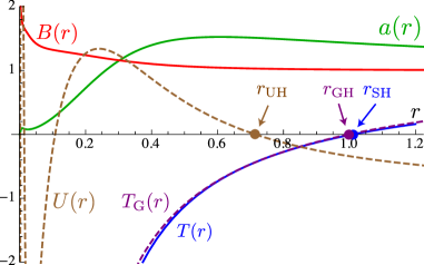
Figure 1: Black hole in the æ-theoryEABH . The coupling constants are set to $c_{13}=0.100,c_{2}=-6.135\times 10^{-4},c_{14}=0.100$. We tune the parameter as $a_{2}=1.112\times 10^{-3}$, which gives a regular scalar-graviton horizon. The graviton sound speed and the scalar-graviton’s one are $c_{\rm G}^{2}=1.111$ and $c_{\rm S}^{2}=1.000$. The black hole mass is normalized as $G_{\rm N}M=0.5$.
The blue, red and green curves indicate the functions $T(r),B(r)$ and $a(r)$, respectively. The scalar-graviton horizon is given by $r_{\mathrm{SH}}=1.010$. The dashed purple curve indicates $T_{\rm G}$, from which we find the graviton horizon as $r_{\mathrm{GH}}=0.998$. The dashed brown curve indicates $U(r):=u\cdot\xi$, which zero point gives the position of the universal horizons. The outermost universal horizon radius is $r_{\rm UH}=0.720$.

Since, the scalar-graviton sound speed is set to unity, the scalar-graviton horizon coincides with the metric horizon : $T(r_{\mathrm{SH}})=0$. We find $r_{\mathrm{SH}}=1.010=2.02G_{\rm N}M$, which is a little larger than the Schwarzschild radius.

The graviton horizon locates inside that of the scalar-graviton, i.e., $r_{\mathrm{GH}}=0.998<r_{\mathrm{SH}}$. It is because the graviton sound speed is faster than the scalar-graviton’s one. The most outer universal horizon is formed inside these two horizons, i.e., $r_{\rm UH}=0.720<r_{\mathrm{GH}},r_{\mathrm{SH}}$. Additionally, more than one inner universal horizons is formed due to the rapid oscillatory behavior of the function $U(r)$ near the central singularity. It means, this solution has a causally disconnected region for low energy particles even if the particle with $z\neq 1$ Lifshitz scaling is taken into account . In this sense, this solution is regarded as a black hole in the low-energy infrared limit.

The important point of this solution is that a physical singularity generally appears on the scalar-graviton horizon (= the metric horizon in the present case), if we do not tune the parameter $a_{2}$. In order to regularize the scalar-graviton horizon, we must choose an appropriate value for the parameter $a_{2}$ as a boundary condition, which is $a_{2}=1.112\times 10^{-3}$. Then, the function $B_{[\ae]}$, which is the “coefficient” of $1/T_{\rm S}$ in the evolution equation of $B(r)$, must vanish on the scalar-graviton horizon $r=r_{\mathrm{SH}}$. We present the detailed analysis of the regularity on the horizons in Appendix C. As a result, for a regular $\ae$-black hole solution, there remains only one free parameter $T_{1}$, which is associated with the black hole mass, just as is the case of the Schwarzschild solution in general relativity.

IV.2 black hole solutions with Lifshitz scaling :
the case of $\beta_{1}\neq 0$ and $g_{2}=\beta_{2}=0$

When the higher-order aether correction $\dot{u}^{4}$ is taken into account, i.e. $\beta_{1}\neq 0$ the solution turns to depend on $a_{2}$ as well as $T_{1}$ unlike æ-black holes. Therefore one may consider the ultraviolet correction $\dot{u}^{4}$ does cure the singular behavior on the scalar-graviton horizon appeared for the infrared-limit theory. In fact, if we assume only $\dot{u}^{4}$ term ($g_{2}=\beta_{2}=0$), we find that there is no singular behavior on any horizon in general. The detailed discussion is developed in Appendix. C.

In this subsection, we consider the case of $\beta_{1}\neq 0$ with $g_{2}=\beta_{2}=0$. There are five types of “black hole” solutions, which are classified in two dimensional parameter space, namely, in $(a_{2},\beta_{1})$ plane. Note that we use the unit of $T_{1}=-1$. We give a classification of these solutions in TABLE 1, which phase diagram of these solutions is shown in Fig. 2.

	solution	region	horizons	singularity	BH
	$\bm{iBH}$ (i)	I(i)	$r_{\mathrm{GH}}<r_{\mathrm{SH}}$ & no $r_{\rm UH}$	$r=0$	$\Delta$
	$\bm{iBH}$ (ii)	I(ii)	$r_{\mathrm{GH}}<r_{\mathrm{SH}}$ & no $r_{\rm UH}$	$0<r<r_{\mathrm{GH}}$	$\Delta$
	$\bm{uBH}$ (i)	II(i)	$r_{\rm UH}<r_{\mathrm{GH}}<r_{\mathrm{SH}}$	$r=0$	$\bigcirc$
	$\bm{uBH}$ (ii)	II(ii)	$r_{\rm UH}<r_{\mathrm{GH}}<r_{\mathrm{SH}}$	$0<r<r_{\rm UH}$	$\bigcirc$
	$\bm{iTS}$	III	no horizons	$r=r_{\mathrm{SH}}$	$\times$
	$\bm{tNS}$	IV	no horizons	$r=0$	$\times$

Table 1: The classification of the solution for the case of $\beta_{1}\neq 0$ with $\beta_{2}=g_{2}=0$. The region I-IV correspond to the areas shown in Fig. 2. $r_{\mathrm{SH}},r_{\mathrm{GH}}$ and $r_{\rm UH}$ are the positions of the scalar-graviton horizon, the graviton horizon, and the universal horizon, respectively. $\Delta$ means that the solution describes a black hole for gravitons and scalar-gravitons, but may becomes naked for high-energetic Lifshitz scaling test particles with $z>1$.

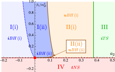
(a) The phase diagram of the solutions

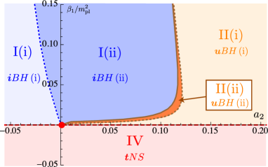
(b) The enlarged phase diagram near the æ-black hole

Figure 2: The phase diagram of the solution in the ($a_{2},\beta_{1}$) parameter plane, where The coupling constants are chosen as the same as Fig.1. The red dashed line which is $\beta_{1}=0$ indicates the case of æ-theory. The æ-black hole with a regular scalar-graviton horizon is shown by the red circle. The genuine black hole solutions which possess the universal horizon are discovered in the region II(i) and II(ii).

We explain each solution in due order:
(1) $\bm{iBH}$ (i) [an infrared black hole with a central singularity]: If $\beta_{1}$ and $a_{2}$ are set to be in the light blue colored region in Fig. 2 (region I(i)), we find a kind of black hole which possesses the graviton horizons. The typical numerical example is shown in Fig. 3(a).

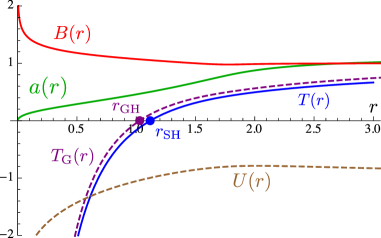
(a) The evolution of the each components of the metric and aether.

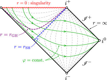
(b) The Carter-Penrose diagram

Figure 3: The typical example of $\bm{iBH}$ (i) (region I(i)). In the top figure (a), We choose $(a_{2},\beta_{1}/m_{\mathrm{pl}}^{2})=(-1.000,1.000)$. The remaining coupling constants and the boundary conditions are set to the same values as those of Fig. 1. The blue, red and green curves indicate the functions $T(r),B(r)$ and $a(r)$, respectively. The dashed purple and dashed brown curves indicate $T_{\rm G}$ and $U(r):=u\cdot\xi$. The graviton horizon is found at $r_{\mathrm{GH}}=1.030$, while the scalar-graviton horizon exists at $r_{\mathrm{SH}}=1.120$. Since $U(r)$ does not vanish, there is no universal horizon, namely, no causal boundary. In the bottom figure (b), the dashed curves indicates $r=$constant surface, especially, the blue, purple and brown curves represent the scalar-graviton horizons, the graviton horizons and the universal horizons, respectively. The spacetime singularities are represented by the waving curves. The future (past) null infinity, the future (past) timelike infinity and the spacelike infinity are indicated by $\mathscr{I}^{+}$ $(\mathscr{I}^{-})$, $i^{+}$ $(i^{-})$ and $i^{0}$, respectively. The ultimately excited particle with $z>1$ Lifshitz scaling propagates along the $\varphi=$constant surface, which is indicated by the solid green curves.

There are graviton and scalar-graviton horizons. In the present case, the dispersion relations of graviton and scalar-graviton are given by $\omega^{2}\sim k^{2}$, which means these horizons coincide with æ-theory’s ones. Hence the gravitons and scalar-gravitons cannot escape from the inside of these horizons. For low-energy particles, they also play a role of horizon too. In this sense, one may regard this solution as a type of black hole, which we call an infrared black hole ($\bm{iBH}$).

The spacetime and aether field are regular except at the center. However, since there exists no universal horizon, this solution has no causally disconnected region. The universal horizon turns to be genuine causal boundary due to the Lifshitz scaling with $z\neq 1$. Therefore the singularity at the center is exposed if non-gravitational propagating modes with the $z>1$ Lifshitz scaling are taken into account. Thus we conclude that this solution does not describes a true black hole in the strict sense but a type of naked singularity even if the graviton horizons exist.

To clarify this situation, we shall depict the spacetime structure. Note that the Carter-Penrose diagram itself does not describe the causal structure of the solution due to the lack of Lorentz invariance. However, since it would be useful to understand the spacetime structure, we will show it for this solution. In Fig. 3(b), we illustrate the Carter-Penrose diagram for this solution, in which null rays propagate on $\pm 45\circ$ direction. The metric (and scalar-graviton) horizon, which is one of the horizons in the Carter-Penrose diagram, is a horizon for the $z=1$ Lorentz invariant particles or for the low-energetic infrared particles. For the $z>1$ Lifshitz scaling high-energetic particles, however, it is no longer horizon, but the spacelike universal horizon will take its place.

(2) $\bm{iBH}$ (ii) [an infrared black hole with a singular spherical shell ]: This solution can be found in the deep blue colored region in Fig.2 (region I(ii)). Although graviton and scalar-graviton horizons are formed, a singularity appears at $r=r_{\rm ss}>0$. As mentioned in (1), this singularity is not causally disconnected from infinity due to the absence of the universal horizon. Therefore, although this solution behaves as a black hole for gravitons and scalar-gravitons as well as Lorentz invariant $z=1$ particles, it turns to be a naked singularity for high-energetic particles with the $z>1$ Lifshitz scaling. In this sense, we also classify this solution as $\bm{iBH}$.

The difference from the case (1) is that the singularity shapes a spherical shell rather than a spacetime point with infinitesimal volume in $\bm{iBH}$ (i). In this paper, we shall refer it as a singular shell.

To see the cause of this singularity, we shall focus on the structure of the evolution equation. We find that the evolution equation of $B(r)$ which is a linear-order differential equation with respect to $r$ (see Appendix C) turns to be singular at $r=r_{\rm ss}$. More specifically, the divergence of $B^{\prime}(r)$ results in this type of singularity. The typical numerical example and the Carter-Penrose diagram are shown in Fig. 4(a) and (b), respectively.

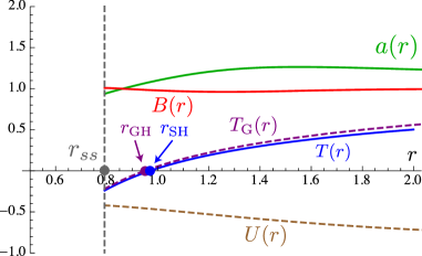
(a) The evolution of the each components of the metric and aether.

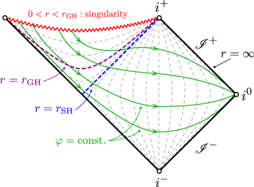
(b) The Carter-Penrose diagram

Figure 4: The typical example of $\bm{iBH}$ (ii) (region I(ii)), In the top figure(a), We choose, $(a_{2},\beta_{1}/m_{\mathrm{pl}}^{2})=(0,1.000)$. The remaining coupling constants and the boundary conditions are set to the same values as those of Fig. 1. The blue, red and green curves indicate the functions $T(r),B(r)$ and $a(r)$, respectively. The dashed purple and dashed brown curves indicate the $T_{\rm G}$ and $U(r)$. The graviton horizon is found at $r_{\mathrm{GH}}=0.949$, while the metric horizon exists at $r_{\mathrm{SH}}=0.970$. The singularity appears at $r_{\mathrm{ss}}=0.792$, which gives the radius of the singular shell. In the bottom figure(b), the conformal structure is depicted. The meaning of the curves and symbols in this figure are same as those of FIG. 3(b).

(3) $\bm{uBH}$ (i) [an ultimate black hole with a central singularity ]: The black hole solution which possesses the graviton, scalar-graviton and universal horizon and no singularity except the center is found in the light orange colored region in Fig. 2 (region II(i)). Since the central singularity is hidden by the universal horizon, this type of the solution is a real black hole. Any particles with the $z>1$ Lifshitz scaling as well as the Lorentz invariant $z=1$ particles cannot escape from the inside of the universal horizon. We then call it an ultimate black hole ($\bm{uBH}$).

We shall show the typical example in Fig. 5(a).

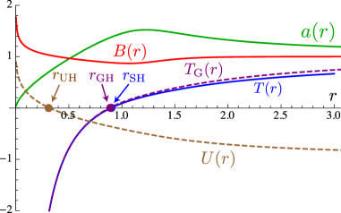
(a) The evolution of the each components of the metric and aether.

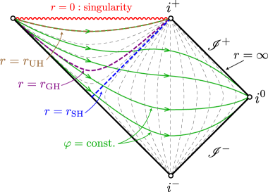
(b) The Carter-Penrose diagram

Figure 5: The typical example of $\bm{uBH}$ (i) (region II(i)). In the top figure(a), we choose $(a_{2},\beta_{1}/m_{\mathrm{pl}}^{2})=(0.200,1.000)$. The remaining coupling constants and the boundary conditions are set to the same values as those of Fig. 1. The blue, red and green curves indicate the functions $T(r),B(r)$ and $a(r)$, respectively. The dashed purple and dashed brown curves indicate $T_{\rm G}$ and $U(r)$. The graviton and the scalar-graviton horizons are found at $r_{\mathrm{GH}}=0.882$ and $r_{\mathrm{SH}}=0.896$, while the universal horizon exists at $r_{\mathrm{UH}}=0.320$. Since there are a universal horizon and a central singularity, this solution is referred to a black hole solution. In the bottom figure(b), the conformal structure is depicted. The meaning of the curves and symbols in this figure are same as those of FIG. 3(b).

This solution is much similar to the æ-black hole illustrated in Fig. 1 except the oscillatory behavior of $U(r)$ near the central singularity. Moreover, we also show the Carter-Penrose diagram of this solution in FIG. 5(b).

(4) $\bm{uBH}$ (ii) [an ultimate black hole with a singular spherical shell ]: When $a_{2}$ and $\beta_{1}$ are in deep orange colored region in Fig.2 (region II(ii)), we find the solution with graviton, scalar-graviton and universal horizon, however, there are a singular shell inside the universal horizon. Since the singular shell is covered by the universal horizon, any information from the singularity never be leaked into the outside. Thus we can regard this type of the solution as a real black hole. Then we also classify this solution as an ultimate black hole ($\bm{uBH}$).

The typical example and the Carter-Penrose diagram of this solution are shown in Fig. 6(a) and (b), respectively.

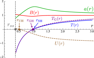
(a) The evolution of the each components of the metric and aether.

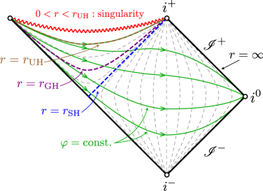
(b) The Carter-Penrose diagram

Figure 6: The typical example of $\bm{uBH}$ (ii) (region II(ii)). In the top figure(a), we choose $(a_{2},\beta_{1}/m_{\mathrm{pl}}^{2})=(0.117,1.000)$. The remaining coupling constants and the boundary conditions are set to the same values as those of Fig. 1. The blue, red and green curves indicate the functions $T(r),B(r)$ and $a(r)$, respectively. The dashed purple and dashed brown curves indicate $T_{\rm G}$ and $U(r)$. The graviton and scalar-graviton horizons are found at $r_{\mathrm{GH}}=0.972$ and $r_{\mathrm{SH}}=0.983$, while the universal horizon exists at $r_{\mathrm{UH}}=0.524$. The singularity appears at $r_{\rm ss}=0.392$, which gives the radius of the singular shell. In the bottom figure(b), the conformal structure is depicted. The meaning of the curves and symbols in this figure are same as those of FIG. 3(b).

(5) $\bm{iTS}$ [an infrared thunderbold singularity]: For the solutions in the light green colored region in Fig. 2 (region III), a singularity always appears at the null Killing horizon of the scalar-graviton. On the singular shell, the function $a(r)$, namely, the $v$ component of the aether field diverges if we set $a_{2}$ to be larger value than a critical one. Furthermore, it is found that the critical value of $a_{2}$ ($\sim 0.377$) which induces the $a(r)$ divergence seems to be universal under any choice of $\beta_{1}$ as shown in Fig. 2). We shall present one typical example and the corresponding Carter-Penrose diagram in Fig. 7. Near the spherical shell with the radius $r_{\rm{SH}}=0.865$, the quadratic scalar of three-dimensional Ricci tensor $\mathcal{R}_{\mu\nu}\mathcal{R}^{\mu\nu}$ diverges. Hence it is a physical singularity.

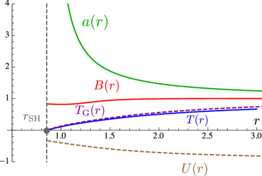
(a) The evolution of each components of the metric and aether.

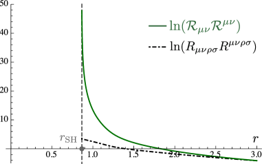
(b) The corresponding evolutions of the curvatures.

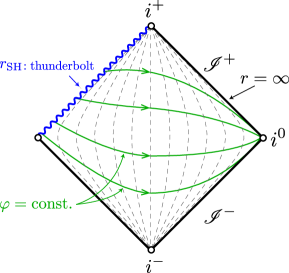
(c) The Carter-Penrose diagram

Figure 7: The typical example of $\bm{iTS}$ (region III). In the top figure(a) and the middle figure(b), we choose $(a_{2},\beta_{1}/m_{\mathrm{pl}}^{2})=(0.500,1.000)$. The remaining coupling constants and the boundary conditions are set to the same values as those of Fig. 1. In the top figure (a), the blue, red and green curves indicate the functions $T(r),B(r)$ and $a(r)$, respectively. The dashed purple and dashed brown curves indicate the $T_{\rm G}$ and $U(r)$. Near the spherical shell with the radius $r_{\rm SH}=0.865$, the quadratic scalar of three-dimensional Ricci tensor $\mathcal{R}_{\mu\nu}\mathcal{R}^{\mu\nu}$ diverges rather than four-dimensional Kretchmann invariant $\mathcal{R}_{\mu\nu}\mathcal{R}^{\mu\nu}$, which are denoted by the solid dark green curve and dot-dashed black curve in the middle figure(b), respectively. In the bottom figure(c), the conformal structure is depicted. The meaning of the curves and symbols in this figure are same as those of FIG. 3(b).

One may wonder why such a singular behavior is occurred on the scalar-graviton horizon. More specifically, from Appendix C, we have known that the basic equations possess no dependence on the negative power of $T_{\rm S}$ unlike the æ-case. Therefore, the scalar-graviton horizon where $T_{\rm S}=0$ should be regular in general. To see in detail, we shall expand the evolution equation of $a(r)$ around $r_{\rm SH}$. From our numerical analysis in Fig. 7, we find $a^{-1}(r_{\mathrm{SH}}+\epsilon)\sim\delta$ and $a^{\prime}(r_{\mathrm{SH}}+\epsilon)\sim\delta^{-2}$, where $\epsilon\ll 1$ and $\delta\ll 1$. In Fig. 7, we have check the divergence numerically at least for $\epsilon\,\mbox{ \raisebox{-4.30554pt}{$\stackrel{{\scriptstyle\textstyle>}}{{\textstyle\sim}}$}}\,1.000\times 10^{-3}$ and $\delta\,\mbox{ \raisebox{-4.30554pt}{$\stackrel{{\scriptstyle\textstyle>}}{{\textstyle\sim}}$}}\,4.132\times 10^{-3}$. Near the singularity, where $T_{\rm S}(r_{\rm SH}+\epsilon):=\Delta_{\epsilon}\ll 1$, the dominant term in the evolution equation of $a(r)$ is given by

$$a^{\prime\prime}(r)\sim{T_{\rm S}^{\prime}(r_{\rm SH})^{3}\over B(r_{\rm SH})^{2}\Delta_{\epsilon}}a^{5}\,.$$ (54)

Thus, we find that $a(r)$ shows singular behavior when $\Delta\to 0$, where the limit gives the scalar-graviton horizon. Since this singularity is due to the aether field rather than the spacetime metric.

This singularity seems to be closely analogous to the thunderbolt singularity. The thunderbolt singularity is proposed in the context of quantum black hole evaporation. In Hawking_Stewart , the thunderbolt singularity is firstly invented in semi-classical analysis of $(1+1)$-dimensional dilaton-coupled gravity with scalar field CGHS which is renormalizable theory of quantum gravity. Furthermore, this type of singularity is also discovered in $(1+1)$-dimensional quantum field theory via complete quantized analysis NS_TB .

In such a situation, a null singularity appears on the event horizon. Although a causally disconnected region is not formed because of the existence of a singularity, this singularity itself is not detected by any outside observer. As a result, it is not a naked singularity. They call it a thunderbolt singularity.

In our case, the singularity of the aether field appears on a Killing horizon is null. Hence it behaves similar to a thunderbolt singularity for Lorentz invariant $z=1$ particles. We call it an infrared thunderbolt singularity ($\bm{iTS}$). The thunderbolt composes of the singular aether field.

(6) $\bm{tNS}$  [a timelike naked singularity without horizon]:
The singular shell without any horizon is found in the light red colored region in Fig. 2 (region IV), namely, $\beta_{1}<0$. Since the singularity is timelike and there is no horizon, this type of the solution completely exposes its singularity. Note that that singularity is originated from the divergence of the evolution equation $B(r)$ as is the case in $\bm{iBH}$ (ii) and $\bm{uBH}$ (ii).

We shall show the typical example in Fig. 8 .

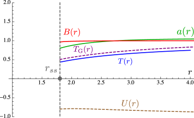
(a) The evolution of each components of the metric and aether.

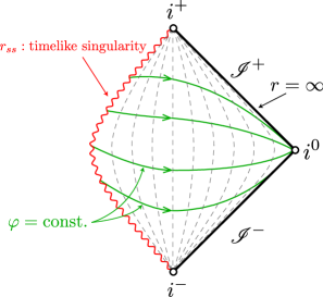
(b) The Carter-Penrose diagram

Figure 8: The typical example of $\bm{tNS}$ (region IV). In the top figure (a), we choose $(a_{2},\beta_{1}/m_{\mathrm{pl}}^{2})=(-1.000,-1.000)$. The remaining coupling constants and the boundary conditions are set to the same values as those of Fig. 1. The blue, red and green curves indicate the functions $T(r),B(r)$ and $a(r)$, respectively. The dashed purple and dashed brown curves indicate the $T_{\rm G}$ and $U(r)$. Note that this solution shows singular behavior at $r_{\rm ss}=1.804$. In the bottom figure (b), the conformal structure is depicted. The meaning of the curves and symbols in this figure are same as those of FIG. 3(b).

IV.3 Ultimate thunderbolt singularity ($\bm{uTS}$)
: the case of $g_{2}\neq 0$ and $\beta_{1}=\beta_{2}=0$

Next, we consider only the spatial higher curvature correction term $\mathcal{R}^{2}$ to take into account the back reaction effect of the Lifshitz scaling in the high energy limit. That is the case of $g_{2}\neq 0$ and $\beta_{1}=\beta_{2}=0$. From the discussion in section III.2, the graviton horizon does not change and its position is still at $r_{\mathrm{GH}}$ where $T_{\rm G}(r_{\mathrm{GH}})=0$. On the other hand, the scalar-graviton horizon is shifted from the Killing horizon to the universal horizon because of $k^{4}$ term in the sound speed (53).

We first assume $g_{2}<0$. In Fig. 9(a), one numerical solution is shown for $g_{2}=-1$. The setting of the coupling constants and the boundary conditions are the same as those of Fig. 1 except $g_{2}=-1$. Notably, we find that a singular behavior on the metric horizon found for untuned arbitrary value of $a_{2}$ in the æ-gravity theory vanishes. The metric horizon turns to be regular for any value of $a_{2}$. Instead, a singular behavior is found inside the metric horizon. The $(v,r)$ component of the metric, $B(r)$ vanishes there. The aether field $u^{\mu}$ aligns perpendicular to the timelike Killing vector $\xi^{\mu}$ near the singular point, which corresponds to the universal horizon with $u\cdot\xi=0$.

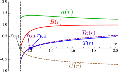
(a) The evolution of each components of metric and aether.

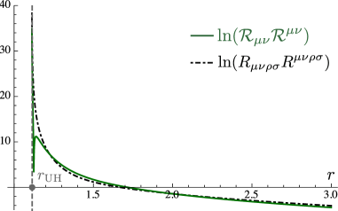
(b) The corresponding evolution of the curvatures.

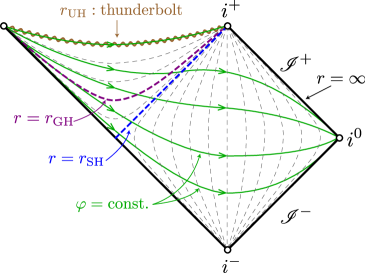
(c) The Carter-Penrose diagram

Figure 9: The spherically symmetric solution with higher spatial curvature correction. The setting of the coupling constants and the boundary conditions are the same as those of Fig. 1 except $g_{2}/m_{\mathrm{pl}}^{2}=-1.000$. In the top figure (a), the blue, red and green curves indicate the functions $T(r),B(r)$ and $a(r)$, respectively. The dashed purple and dashed brown curves indicate the $T_{\rm G}$ and $U(r)$. The graviton horizon is found at $r_{\mathrm{GH}}=1.248$, while the metric horizon exists at $r_{\rm KH}=1.250$. The calculation has been broken down at $r_{\mathrm{UH}}=1.157$ where $U(r)$ approaches to zero. In the middle figure (b), the dotted gray and dotted black curves indicate $\ln(R_{\mu\nu\rho\sigma}R^{\mu\nu\rho\sigma})$ and $\ln(\mathcal{R}_{\mu\nu}\mathcal{R}^{\mu\nu})$, respectively. In the bottom figure (c), the conformal structure is depicted. The meaning of the curves and symbols in this figure are same as those of FIG. 3(b).

We calculate the four-dimensional Kretchmann invariant $R_{\mu\nu\rho\sigma}R^{\mu\nu\rho\sigma}$ and the quadratic scalar of the three-dimensional Ricci tensor $\mathcal{R}_{\mu\nu}\mathcal{R}^{\mu\nu}$, which are shown in Fig. 9(b). Near the singular point, those two scalar functions diverge. Thus, this singular point is a physical singularity rather than a coordinate singularity. So we find that the universal horizon becomes singular. Additionally, the structure of this spacetime is depicted in FIG. 9(c).

What causes this type of singularity ? In order to clarify this question, we first show the relation between $g_{2}$ and the radii of the graviton horizon $r_{\mathrm{GH}}$, the metric horizon $r_{\rm KH}$ and the singular universal horizon $r_{\rm UH}$ in Fig. 10. We also give the detailed data of the singular universal horizon radius $r_{\rm UH}$ near $g_{2}=0$ in Table 2.

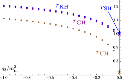
Figure 10: The relation between several horizon radii and $g_{2}$. The coupling constants and the boundary conditions are the same as Figs. 1 and 9 except $g_{2}$. The purple, blue and brown star marks indicate the graviton horizon radius $r_{\mathrm{GH}}$, the scalar-graviton horizon radius $r_{\mathrm{SH}}$ and the singular universal horizon radius $r_{\rm UH}$ in the æ-gravity theory, respectively. The purple, blue and brown round circles indicate the graviton horizon radius $r_{\mathrm{GH}}$, the metric horizon radius $r_{\rm KH}$, and the radius of the singular universal horizon $r_{\rm UH}$. Numerically the position of $r_{\rm UH}$ is evaluated at the point of $U(r)=-0.025$, because $U(r)=0$ is singular.

	$g_{2}/m_{\mathrm{pl}}^{2}$	$r_{\rm UH}$	$g_{2}/m_{\mathrm{pl}}^{2}$	$r_{\rm UH}$
	0	0.7200	$-5.00\times 10^{-4}$	0.7944
	$-1.00\times 10^{-4}$	0.7783	$-6.00\times 10^{-4}$	0.7962
	$-2.00\times 10^{-4}$	0.7854	$-7.00\times 10^{-4}$	0.7977
	$-3.00\times 10^{-4}$	0.7893	$-8.00\times 10^{-4}$	0.7990
	$-4.00\times 10^{-4}$	0.7922	$-9.00\times 10^{-4}$	0.8002

Table 2: The detailed value of $r_{\mathrm{UH}}$ for near $g_{2}=0$. The coupling constants and the boundary conditions are same as Fig. 10 except $g_{2}$. The values of $r_{\mathrm{UH}}$ are evaluated at the point where $U(r)=-0.025$.

From these results, we find that the universal horizon radii change smoothly from $g_{2}=0$ case to $g_{2}\neq 0$ cases.

One may wonder whether it can be regular if we tune the free parameter $a_{2}$ just as the scalar-graviton horizon in the æ-gravity theory. To see this, we shall perform the expansion of the basic equations around the universal horizon. Focusing on the coefficients of the most highest $r$ derivative terms, $T^{\prime\prime\prime}(r)$, $B^{\prime\prime\prime}(r)$ and $a^{\prime\prime\prime}(r)$ terms in the $(\theta,\theta)$ component of the Einstein equation, we find all of them have been vanished at the universal horizon (see Appendix.C). This result does not depend on the value of $a_{2}$. This fact means that the singularity on the universal horizon cannot be remedied by tuning the free parameter $a_{2}$ unlike the æ-case. While there is no singular behavior on the scalar-graviton horizon $r_{\mathrm{SH}}$ in the infrared limit where $T_{\rm S}$ vanishes.

Hence it is not quite unnatural to consider that the singular behavior which appears on the scalar-graviton radius with $T_{\rm S}=0$ in the infrared limit is shifted to the universal horizon when we include the higher curvature term from the Lifshitz scaling. Namely, the dispersion relation of the scalar-graviton with nonzero $g_{2}$ gives the infinite sound speed of the scalar-graviton. The similar situation is found for the exact solution with $c_{14}=0$ in the æ-gravity theory mec_UH , for which the sound speed of the scalar-graviton (46) becomes infinite and the scalar-graviton horizon coincides with the universal horizon. In this case, however, this singularity can be removed by choosing an appropriate value of $a_{2}$.

We shall turn our attention to the physical interpretation of this solution. Recall that the universal horizon is defined by surface where $u\cdot\xi=0$, i.e., a static limit for the ultimately excited dispersive particle with $z\neq 1$ Lifshitz scaling. In other words, only the particle which possesses infinite energy can stay on the surface, and any future-directed signal on the surface cannot goes outward even if the particle is spacelike with infinite energy. Namely, the information on the universal horizon must not be leaked out to outside of the horizon. Although this solution cannot be regarded as a black hole solution whose spacetime singularity is isolated by an event horizon, the cosmic censorship hypothesis is not violated on this account.

This singularity is very similar to the thunderbolt singularity if we replace a null event horizon with a spacelike universal horizon. The universal horizon is a real horizon for the $z>1$ Lifshitz scaling particles. So the singular universal horizon cannot be detected by any outside observers. Although there is no causally disconnected region, it is not a naked singularity. We then call it a ultimate thunderbolt singularity ($\bm{uTS}$). We may speculate that the appearance of the thunderbolt singularity on the universal horizon via $\mathcal{R}^{2}$ term indicates quantum gravitational loop correction in the Lorentz violating system as in quantization of the Lorentz invariant system with a thunderbolt singularity.

Besides, one may wonder about solutions for the positive value of $g_{2}$. In fact, this case is less interesting. Namely, all black hole horizons which exist in the case of $g_{2}=0$ completely disappear. The property of the solution is quite unphysical, i.e., the functions $T(r)$ and $B(r)$ show positive divergence at smaller radius $r\sim\mathcal{O}(10G_{\rm N}M)$, while the function $a(r)$ drops to zero without forming any horizon. In other words, there does not exist any type of black holes discussed before (See Fig. 11).

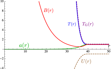
Figure 11: The typical example of the solution with positive $g_{2}$. We set $a_{2}=1.123\times 10^{-3}$ and $g_{2}/m_{\mathrm{pl}}^{2}=1.000$. The remaining coupling constants and the boundary conditions are set to the same values as those of Fig. 9. The blue, red and green curves indicate the functions $T(r),B(r)$ and $a(r)$, respectively. The dashed purple and dashed brown curves indicate the $T_{\rm G}$ and $U(r)$. The function $a(r)$ drops to zero, while $T(r)$ and $B(r)$ diverges for smaller radius $r$.

IV.4 Solutions with $z=2$ Lifshitz scaling terms
: the case of $g_{2}\neq 0$ and $\beta_{1},\beta_{2}\neq 0$

If we have only $\dot{u}^{4}$ term, we find $\bm{uBH}$ for an appropriate value of $a_{2}$. The universal horizon is not singular. On the other hand, when we have only $\mathcal{R}^{2}$ term, the universal horizon becomes singular, giving a thunderbolt singularity $\bm{uTS}$. One may wonder what happens if both $z=2$ Lifshitz scaling terms, $\dot{u}^{4}$ and $\mathcal{R}^{2}$, exist ($g_{2}\neq 0$ and $\beta_{1}\neq 0$). Since $\mathcal{R}^{2}$ and $\dot{u}^{2}\mathcal{R}$ give the highest derivative terms in the equation of motion, namely, $T^{\prime\prime}(r)$, $B^{\prime\prime}(r)$ and $a^{\prime\prime\prime}(r)$, the $\bm{uTS}$ spacetime with $|\beta_{1}|\ll|g_{2}|$ is not so different from the original one. On the other hand, if $|\beta_{1}|$ is not so small compared with $|g_{2}|$, the spacetime tends to generate a singularity caused by the aether field. More specifically, a singular spherical shell appears before forming the thunderbolt singularity on the universal horizon. Thus, we can only find $\bm{iBH}$ (ii) and $\bm{tNS}$ spacetime in this situation.

Finally, we mention the case of $\beta_{2}\neq 0$. Although we have shown that there must not exist a regular universal horizon in this case (see Appendix C), any horizons cannot be found as far as our numerical analysis. In other words, the spacetime produces a singular spherical shell before forming any horizon, namely, $\bm{tNS}$ solution.

V Properties of Solutions

We shall discuss the properties of obtained black hole and thunderbolt singularity solutions from several view points.

V.1 Distribution of the aether field

In our solutions, there are two free parameters, $M$ and $a_{2}$. The mass is a conserved quantity, which characterizes the solution. Althogh the different value of $a_{2}$ gives the different solution, $a_{2}$ may not correspond to any conserved quantity. In order to understand the physical meaning of $a_{2}$, we consider the energy density distribution of the aether field.

We define the effective energy density and pressures of the aether field by

$$\rho_{\rm\ae} := T^{\rm[\ae]}_{\mu\nu}u^{\mu}u^{\nu}\,,$$

$$P^{[r]}_{\rm\ae} := T^{\rm[\ae]}_{\mu\nu}s^{\mu}s^{\nu}\,,$$

$$P^{[\perp]}_{\rm\ae} := {1\over 2}T^{\rm[\ae]}_{\mu\nu}(g^{\mu\nu}+u^{\mu}u^{\nu}-s^{\mu}s^{\nu})\,.$$ (55)

When we calculate $\rho_{\rm\ae},P^{[r]}_{\rm\ae},P^{[\perp]}_{\rm\ae}$ we use the Einstein equations:

$$8\pi GT^{\rm[\ae]}_{\mu\nu}=G_{\mu\nu}\,.$$ (56)

It makes easy to evaluate $T^{\rm[\ae]}_{\mu\nu}$ once we obtain the solutions.

First we show $\rho_{\rm\ae}$, $P^{[r]}_{\rm\ae}$, and $P^{[\perp]}_{\rm\ae}$ for the æ-black hole in Fig. 12 as a reference.

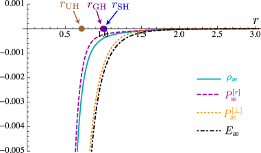
Figure 12: The distributions of the aether cloud for the æ-black hole. The solid cyan, dashed magenta, dotted yellow and dot-dashed black curve indicate $\rho_{\rm\ae}$, $P^{[r]}_{\rm\ae}$, $P^{[\perp]}_{\rm\ae}$ and $E_{\rm\ae}$, respectively. The coupling constants and the boundary conditions are set to the same values as those of FIG. 1.

In the æ-black hole, all aether quantities are always negative. Additionally, the following quantity $E_{\rm\ae}$ is introduced in order to examine the strong energy condition,

$$E_{\rm\ae} := \left(T^{\rm[\ae]}_{\mu\nu}-{1\over 2}T^{\rm[\ae]}g_{\mu\nu}\right)u^{\mu}u^{\nu}$$ (57)

$$= {1\over 2}\left(3\rho_{\rm\ae}-P^{[r]}_{\rm\ae}-2P^{[\perp]}_{\rm\ae}\right)\,.$$

It is also negative definite, which means that the strong energy condition is broken.

We then show $\rho_{\rm\ae}$, $P^{[r]}_{\rm\ae}$, $P^{[\perp]}_{\rm\ae}$ and $E_{\rm\ae}$ for each solution in Figs. 13 and 14.

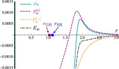
(a) $\bm{iBH}$ (i)

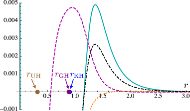
(b) $\bm{uBH}$ (i)

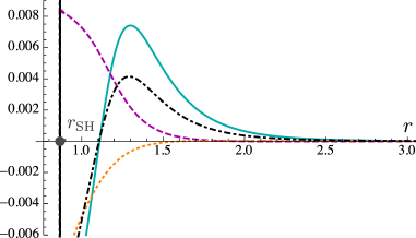
(c) $\bm{iTS}$

Figure 13: The distributions of the aether cloud for the solutions which are found in $\beta_{1}\neq 0$, $\beta_{2}=g_{2}=0$. We illustrate the typical example of ${\bm{iBH}}$ (i) (the top figure (a)), the ${\bm{uBH}}$ (i) (the middle figure (b)) the ${\bm{iTS}}$ (the bottom figure (c)) instead of showing all kind of the solutions. The solid cyan, dashed magenta, dotted yellow and dot-dashed black curve indicate $\rho_{\rm\ae}$, $P^{[r]}_{\rm\ae}$, $P^{[\perp]}_{\rm\ae}$ and $E_{\rm\ae}$, respectively. The coupling constants and the boundary conditions for (a), (b) and (c) are set to the same values as those of FIG. 3, 5, and 7, respectively.

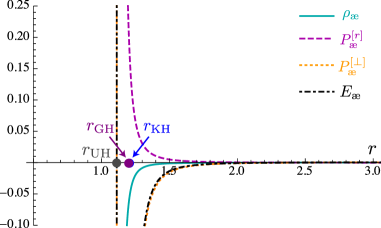
Figure 14: The distributions of the aether cloud for the $\bm{uTS}$ spacetime. The solid cyan, dashed magenta, dotted yellow and dot-dashed black curve indicate $\rho_{\rm\ae}$, $P^{[r]}_{\rm\ae}$, $P^{[\perp]}_{\rm\ae}$ and $E_{\rm\ae}$, respectively. The coupling constants and the boundary conditions are set to the same values as those of FIG. 9.

When we add the $z=2$ Lifshitz scaling terms, the distribution of the aether field is drastically changed. For the case of $\beta_{1}\neq 0$, $\beta_{2}=g_{2}=0$ (for $\bm{iBH}$, $\bm{uBH}$ and $\bm{iTS}$ spacetime), the localized aether cloud is formed, i.e., $\rho_{\rm\ae}$ and $P^{[r]}_{\rm\ae}$ are localized near the graviton and the scalar-graviton horizons. We may speculate that the positivity of the aether density and radial pressure relax a singular behavior at the scalar-graviton horizon, which exists in æ-theory with general value of $a_{2}$. Note that the strong energy condition is satisfied for some finite radial region. Furthermore, referring FIG. 2 and the aether distribution FIG. 13 (a), (b) and (c), for the larger value of $a_{2}$, the more dense aether cloud forms. As a result, the $\bm{iTS}$ spacetime is emerged in the large $a_{2}$ region due to the gravitational collapse of the aether cloud.

For the case of $g_{2}\neq 0$, $\beta_{1}=\beta_{2}=0$ (for $\bm{uTS}$ spacetime), the distribution is different. Referring FIG. 14, although the radial pressure is positive, the energy density becomes negative. The strong energy condition is broken in the whole spacetime. Note that the radial pressure diverges where the shell singularity appears.

V.2 Preferable Black Holes

Although black hole thermodynamics in æ-gravity theory has been discussed in the last decade, the complete understanding have not yet achieved. Hence, in this section, we only discuss which solution is more preferable from the view point of the thermodynamical stability

In the previous section, we find two-parameter “black hole” solutions: One free parameter is a black hole mass $M$, which is used to normalize the variables, and the other free parameter is $a_{2}$. However we have only one Noether charge with respect to time translational symmetry, which is the black hole mass $M$ given by (44). As we showed in the previous subsection, the parameter $a_{2}$ describes the distribution of the aether field, but does not provide a conserved quantity. It just describes a cloud of the aether field around a black hole or a thunderbolt singularity. $a_{2}$ describes a different configuration of the aether cloud.

Hence, fixing a black hole mass $M$ and changing $a_{2}$, we may find most preferable configuration of the aether field, which gives a stable solution. To find such a solution, we adopt the view point of thermodynamical stability, i.e., we assume that the maximum entropy determines the stable configuration.

However, the definition of the black hole entropy is unclear due to the unavailability of Wald’s Noether charge method on the black hole horizons in æ-theory and its extension. In addition, according to Wald_entropy , the black hole entropy is modified by the higher curvature terms. Namely, it is given by the integration of functional derivative of the action with respect to four dimensional Riemann tensor denoted by $E^{\mu\nu\rho\sigma}$ over the bifurcation surface $\mathcal{B}$. In our case,

$$E^{\mu\nu\rho\sigma}=(1-\beta_{2}\dot{u}^{2}-2g_{2}\mathcal{R})g^{\mu\rho}g^{\nu\sigma}\,.$$ (58)

Unfortunately, this modification factor $(1-\beta_{2}\dot{u}^{2}-2g_{2}\mathcal{R})$ diverges near the universal horizon due to the singular behavior of the three curvature $\mathcal{R}$.

Hence here we consider only the case without the higher-curvature correction terms ($g_{2}=\beta_{2}=0$). Then we simply assume the black hole entropy is given by the area of the horizon $\mathcal{A}(r_{H})$, where $r_{H}$ is one of horizon radii . If we find more appropriate definition of the black hole entropy, our result would be changed.

Here we adopt the universal horizon to evaluate the black hole entropy:

$$\mathcal{S}_{\rm uBH}:={\mathcal{A}(r_{\rm UH})\over 4G_{\rm N}}={\pi r^{2}_{\rm UH}\over G_{\rm N}}\,.$$ (59)

In Fig. 15, we show the radii of the universal horizon $r_{\mathrm{UH}}$ with respect to $a_{2}$ for $\bm{uBH}$ spacetime.

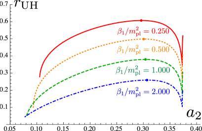
Figure 15: The radii of the universal horizons $r_{\mathrm{UH}}$ with respect to $a_{2}$ for $\bm{uBH}$ spacetime. The solid red, dotted orange, dashed green and dot-dashed blue curve indicate for $\beta_{1}/m_{\mathrm{pl}}^{2}=0.250,0.500,1.000$ and $2.000$ case, respectively. The remaining coupling constants and the boundary conditions are set to the same values as those of Fig. 1. The points which give the largest value of $r_{\mathrm{UH}}$ for each $\beta_{1}$ are indicated by the circle plot on the each curves. The turning point where the curve has the sharp edge is given by $a_{2\mathrm{(turn)}}=0.373$ for every $\beta_{1}$.

The property of the universal horizon is summarized as follows : Each universal horizon radius is a convex upward function with respect to $a_{2}$ except the right edge. The maximum value of black hole entropy for each value of $\beta_{1}$ is given at the top of the convex, which is denoted by $r_{\mathrm{UH}\mathrm{(max)}}$. At the end of the convex function which is called a ”turning point” denoted by $a_{2\mathrm{(turn)}}$, the function sharply bounce and turns to increase until the regular universal horizon disappears. Beyond this point, we find $\bm{iTS}$ solution. Remarkably, the value of $a_{2}$ at turning point and the right edge of these plot are invariant with respect to $\beta_{1}$, which are given by $a_{2\mathrm{(turn)}}=0.373$ and $a_{2(\mathrm{end})}=0.377$, respectively. Note that $a_{2(\mathrm{end})}$ corresponds to the border between $\bm{uBH}$ and $\bm{iTS}$ spacetimes.

We give the detailed data of the thermal quantities with the maximum entropy and at the turning point for each value of $\beta_{1}$ in TABLE 3.

	$\beta_{1}/m_{\mathrm{pl}}^{2}$	$a_{2\mathrm{(max)}}$	$r_{\mathrm{UH(max)}}$	$a_{2\mathrm{(turn)}}$	$r_{\mathrm{UH(turn)}}$
	$0.250$	$0.296$	$0.607$	$0.373$	$0.345$
	$0.500$	$0.301$	$0.499$	$0.373$	$0.262$
	$1.000$	$0.304$	$0.380$	$0.373$	$0.178$
	$2.000$	$0.307$	$0.259$	$0.373$	$0.103$

Table 3: the detailed data of the universal horizon radii at the maximum point and at the turning point for each value of $\beta_{1}$.

When we take the maximum value of the universal horizon radii with respect to $a_{2}$, we may find the most preferable black hole solution for a given mass $M$. It is because such a maximum point may give a stable solution from the view point of the black hole thermodynamics.

Then we find a series of these most preferable black hole solutions in terms of $M$. In Fig. 16, we plot the horizon radii of such a black hole v.s. the gravitational mass $M$ for $\beta_{1}/m_{\mathrm{pl}}^{2}=1$. Additionally, that of the æ-black hole, namely, $\beta_{1}=\beta_{2}=g_{2}=0$ case, are also shown as reference.

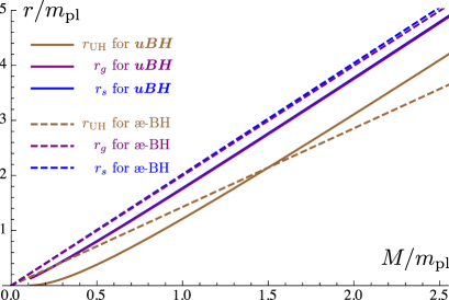
Figure 16: The mass dependence of the horizon radii for the most preferable black hole solutions with $\beta_{1}/m_{\mathrm{pl}}^{2}=1$ are indicated by solid curves. $a_{2}$ is fixed so that the maximum universal horizon radii is obtained. The remaining coupling constants and the boundary conditions are set to the same values as those of Fig. 1. The brown, purple and blue curves indicate the radii of the universal horizon, the graviton horizon and the scalar-graviton horizon, respectively. The radius of the $\bm{uBH}$ universal horizon turn to be greater than that of æ-black hole in $M>M_{\mathrm{crit}}=1.497m_{\mathrm{pl}}$ region.

For all horizons (the graviton, scalar-graviton and universal horizons) of the æ-black hole, their radii seem to increase linearly in terms of the mass $M$, which is the same as that of Schwarzschild solution.

Whereas, for our $\bm{uBH}$, the universal horizon radius increases with a higher power-law function of $M$ than the linear one in the small mass region, and it approaches a linear function for large values of $M$. The $\bm{uBH}$ universal horizon radius is smaller than æ-black holes’s one for $M>M_{\mathrm{crit}}=1.497m_{\mathrm{pl}}$. We shall refer $M_{\mathrm{crit}}$ as a critical mass. Note that the universal horizon radius seems to vanish for small value of $M$, but it is not clear whether it vanishes at a finite mass $M_{\rm min}(>0)$, or at $M=0$.

One may wonder whether our ${\bm{u}BH}$ solution will recover the æ-black hole or not when $\beta_{1}$ approaches to zero. To see this, we give the detailed data of $r_{\rm{UH(max)}}$ and corresponding $a_{2\mathrm{(max)}}$ near $\beta_{1}=0$ in Table 4.

	$\beta_{1}/m_{\mathrm{pl}}^{2}$	$a_{2\mathrm{(max)}}$	$r_{\mathrm{UH(max)}}$
	$0$	$1.112\times 10^{-3}$	$0.720$
	$0.001$	$0.229$	$1.001$
	$0.005$	$0.248$	$0.949$
	$0.010$	$0.259$	$0.916$
	$0.050$	$0.281$	$0.799$
	$0.100$	$0.288$	$0.727$

Table 4: The detailed values of $r_{\rm{UH}}$ and corresponding $a_{2}$ of the most preferable $\bm{uBH}$ solutions for $\beta_{1}\ll 1$. The case of $\beta_{1}=0$ corresponds to the æ-black hole. The coupling constants and the boundary conditions are set to the same values as those of FIG. 1.

From this table, we find that the value of $a_{2_{\mathrm{(max)}}}$ gradually decreases as $\beta_{1}\rightarrow 0$. Whereas, the maximum value of the universal horizon radius increases in such a limit. Thus, we can conclude that the $\bm{uBH}$ solution cannot be smoothly connected to the æ-black hole.

V.3 Smarr’s formula and Black Hole Temperature

Concerning the black hole first law in æ-theory, it is found that the aether field prevents from establishing the black hole mass-entropy relation on the Killing horizonnoether_charge_ae via Noether charge methodNC_is_entropy ; Wald_entropy . Notwithstanding, the Smarr’s formula in æ-theory has been proposed only in static and spherically symmetric configurationmec_UH , which is established by applying Gauss’s law to the aether field equation. It is found that the aether portion of the basic equation can be reduced to Maxwell-like form in static and spherically symmetric spacetime :

$$\nabla_{\alpha}\mathcal{F}^{\alpha\mu}=0\,,$$ (60)

where, $\mathcal{F}_{\mu\nu}$ is given by

$$\mathcal{F}_{\mu\nu} := 2qu_{[\mu}s_{\nu]}\,,$$ (61)

$$q := \left[{c_{14}\over 2}-c_{13}\right](\dot{u}\cdot s)(u\cdot\xi)+(1-c_{13})\kappa$$ (62)

$$+{c_{123}\over 2}(\nabla\cdot u)(s\cdot\xi)\,,$$

$s^{\mu}$ is a spacelike unit vector perpendicular to $u^{\mu}$ and a surface gravity $\kappa$ which is given by $\xi^{\alpha}\nabla_{\alpha}\xi^{\mu}=\kappa\xi^{\mu}$ is equivalent to the following form due to a spacetime symmetry :

$$\kappa=\sqrt{-{1\over 2}(\nabla_{\alpha}\xi_{\beta})(\nabla^{\alpha}\xi^{\beta})}\,.$$ (63)

Note that the structure of (60) is similar to Maxwell’s equation, thus, we can perform the flux integration. According to Gauss’s law, the integration of $\mathcal{F}_{\mu\nu}$ over $\mathcal{B}_{r}$ which is a two sphere at radius $r$ must produce same value for any $r$. Considering the integration over spatial infinity $\mathcal{B}_{\infty}$ and $\mathcal{B}_{r}$, then we obtain

$$M=q(r){\mathcal{A}(r)\over 4\pi G_{\rm N}}\,,$$ (64)

where $\mathcal{A}(r):=4\pi r^{2}$ is a surface area of $\mathcal{B}_{r}$. Note that this relation is held for any $r$. When we evaluate the r.h.s. of Eq. (64), we find the Smarr’s formula:

$$M=\mathcal{T}^{(\ae)}_{\rm uBH}\mathcal{S}_{\rm uBH}\,,$$ (65)

where $\mathcal{T}^{(\ae)}_{\rm uBH}=q(r_{\rm UH})/\pi$ is a black hole temperature.

Turning to our attention to the case of including higher curvature and aether effects, although the Maxwell-like aether equation is not found, we may obtain the relation between the black hole mass and the entropy (or the area of the universal horizon) by evaluating the deviation from the æ-black hole’s one. Note that our thermodynamical analysis is limited to the black hole solution only with $\beta_{1}$ term. If we consider the surface gravity or black hole temperature on the singular horizon, these quantities must diverge. Thus, we shall not discuss the solutions without a regular universal horizon.

We shall presume the mass-entropy relation as follows:

$$M = \mathcal{T}^{(z=2)}_{\rm uBH}\mathcal{S}_{\rm uBH}$$ (66)

where $\mathcal{T}^{(z=2)}_{\rm uBH}:=\mathcal{T}^{(\ae)}_{\rm uBH}+\delta\mathcal{T}^{(z=2)}_{\rm uBH}$. $\delta\mathcal{T}^{(z=2)}_{\rm uBH}$ is introduced as the correction by the $z=2$ Lifshitz scaling term from the æ-black hole temperature.

In Fig. 17, we show the mass-temperature relation of the most preferable black hole solutions defined in the previous subsection. We also show æ-casemec_UH as a reference.

Figure 17: The mass-temperature on the universal horizon for the most preferable black hole solutions. The solid red, dotted orange, dashed green and dot-dashed blue curves indicate the temperatures $\mathcal{T}^{(z=2)}_{\rm uBH}$ for $\beta_{1}/m_{\mathrm{pl}}^{2}=0.250,0.500,1.000$ and $2.00$, respectively. The values of $a_{2}$ for each case are fixed so that the maximum universal horizon radii is obtained. The remaining coupling constants and the boundary conditions are set to the same values as those of Fig. 1. The æ-case is also shown as a reference, which is indicated by the two-dot chain black line. The critical mass for each $\beta_{1}$ are indicated by the colored dot.

From this plot, we find that the æ-black hole temperature seems to be inversely proportional to the black hole mass $M$, which is the same as the Schwarzschild black hole in GR. Whereas, that of our $\bm{uBH}$ solution is clearly far from the inverse $M$ law. More specifically, the black hole temperature of $\bm{uBH}$ turns to be lower than that of æ-case for the range of $M>M_{\mathrm{crit}}$, where $M_{\mathrm{crit}}$ is the critical mass defined in the previous subsection. In TABLE. 5, we show the values of $M_{\mathrm{crit}}$ and corresponding $r_{\mathrm{UH}}$ in terms of $\beta_{1}$.

	$\beta_{1}/m_{\mathrm{pl}}^{2}$	$M_{\mathrm{crit}}/m_{\mathrm{pl}}$	$r_{\mathrm{UH}}/m_{\mathrm{pl}}$
	$1.000$	$1.497$	$2.134$
	$0.900$	$1.420$	$2.029$
	$0.800$	$1.339$	$1.913$
	$0.700$	$1.253$	$1.789$
	$0.600$	$1.160$	$1.656$
	$0.500$	$1.059$	$1.512$
	$0.400$	$0.947$	$1.352$
	$0.300$	$0.820$	$1.171$
	$0.200$	$0.670$	$0.956$
	$0.100$	$0.473$	$0.676$

Table 5: The critical masses and corresponding universal horizon radii in terms of $\beta_{1}$.

From FIG. 17, the temperatures of the $\bm{uBH}$ solutions seem to obey the inverse $M$ law in large $M$ region, while it may decrease exponentially in small $M$ region. To examine this behavior, we shall assume that the mass-temperature relation is given by the following functional form :

$$\mathcal{T}^{(z=2)}_{\rm uBH} \approx \mu\left(e^{\nu/(M-M_{\rm min})}-1\right)$$

$$\sim \begin{cases}\mu e^{\nu/(M-M_{\rm min})}&~{}{\rm for}~{}M-M_{\rm min}\ll\nu\\ \mu\nu/(M-M_{\rm min})&~{}{\rm for}~{}M-M_{\rm min}\gg\nu\end{cases}\,,$$

where $\mu$, $\nu$ and $M_{\rm min}$ are some fitting parameters. Since the universal horizon radius is related to the black hole mass as (66), the universal horizon should disappear when $M=M_{\rm min}$, where $\mathcal{T}^{(z=2)}_{\rm uBH}$ diverges.

The curves in FIG. 17 are approximately reproduced by the above functional form (LABEL:approx_T) if we choose the fitting parameters given in TABLE. 6.

	$\beta_{1}/m_{\mathrm{pl}}^{2}$	$\mu~{}m_{\mathrm{pl}}$	$\nu/m_{\mathrm{pl}}$	$M_{\rm min}/m_{\mathrm{pl}}$	$\mathcal{T}^{(z=2)}_{\rm{uBH}}(M\gg m_{\mathrm{pl}})$
	$0.250$	$0.136$	$0.649$	$6.561\times 10^{-7}$	$0.088/M$
	$0.500$	$0.096$	$0.919$	$9.261\times 10^{-7}$	$0.088/M$
	$1.000$	$0.068$	$1.299$	$9.468\times 10^{-7}$	$0.088/M$
	$2.000$	$0.048$	$1.837$	$9.998\times 10^{-7}$	$0.088/M$
	$0$	N/A	N/A	N/A	$\mathcal{T}^{(\ae)}_{\rm uBH}=0.151/M$

Table 6: The fitting parameters in $\mathcal{T}^{(z=2)}_{\rm uBH}$ and the asymptotic behaviors in large $M$ region for each value of $\beta_{1}$. The coupling constants and the boundary conditions are set to the same values as those of FIG. 17. We also show the temperature of the æ-black hole $\mathcal{T}^{(\ae)}_{\rm uBH}$ as a reference in the bottom line.

In our numerical result, it is found that $M_{\rm min}$ is extremely small, or possibly vanishes. Moreover, it is notable that the values of $\mu\nu$ seem to be universal for $\beta_{1}>0$, namely, all asymptotic behaviors in large $M$ region, which is denoted by $\mathcal{T}^{(z=2)}_{\rm{uBH}}(M\gg m_{\mathrm{pl}})$, are the same, but differs from that of the æ-black hole.

VI conclusion and discussion

Without Lorentz symmetry, the Killing horizon is no longer the event horizon in the static and spherically symmetric spacetime due to the presence of the superluminal propagating modes. However, in the context of the æ-theory or infrared limit of the non-projectable HL gravity, a black hole solution can be still constructed by considering the universal horizon which is a static limit for an instantaneously propagating particle. In this paper, we have studied the backreaction to the black hole solution in æ-theory by the Lifshitz scaling terms. We have analyzed the ultraviolet modification of the æ-black holes including the simple scalar terms with $z=2$ Lifshitz scaling, specifically, the quadratic term of spacial curvature associated with the hypersurface orthogonal aether field ($\mathcal{R}^{2}$), the quartic term of the aether acceleration ($\dot{u}^{4}$), and the product of the spacial curvature and the quadratic term of the aether acceleration ($\dot{u}^{2}\mathcal{R}$).

Only for the case with $\dot{u}^{4}$ term ($\beta_{1}\neq 0$ and $\beta_{2}=g_{2}=0$), we have succeeded in finding a black hole solution with regular universal horizon, which is referred as $\bm{uBH}$. In contrast to the æ-case, the black hole solutions are obtained without tuning the boundary parameter of the aether field $a_{2}$. In other words, $\bm{uBH}$ solutions exist in a finite range in the $(\beta_{1},a_{2})$ parameter plane (see FIG. 2). If we select the parameter $a_{2}$ beyond this range, a singular shell appears before forming a universal horizon. While, considering $\dot{u}^{2}\mathcal{R}$ and/or $\mathcal{R}^{2}$ terms ($\beta_{2}\neq 0$ and/or $g_{2}\neq 0$), any black hole solution with regular universal horizon cannot be constructed due to the divergence of the basic equations on the universal horizon (see Appendix.C). However, including only $\mathcal{R}^{2}$ term with negative $g_{2}$, we have found the solution with a thunderbolt singularity ($\bm{uTS}$), whose universal horizon turns is still singular but the singularity is not observed any outside observers. Although this solution cannot be regarded as a black hole, the cosmic censorship hypothesis is not violated. Since the thunderbolt singularity had been discovered in the context of the quantum gravity in lower dimension, the emergence of this solution is not so strange since the $z=2$ Lifshitz scaling terms are regarded as quantum gravitational corrections.

We then have studied several properties of our solutions including spacetime structures with their Carter-Penrose diagrams. To investigate the physical meaning of $a_{2}$, we have shown the effective energy momentum tensor of the aether field $T^{[\ae]}_{\mu\nu}$, i.e., the effective energy density and pressure. From these results, the parameter $a_{2}$ seems closely related to the distribution of the spherical aether cloud. Namely, large value of $a_{2}$ configures a dense aether cloud and eventually induces a collapse of the aether field, which results in a formation of a ”timelike” singular shell ($\bm{tNS}$). Moreover, we may speculate that regularity on the (infrared limit of) scalar graviton horizon is recovered due to the localization of the aether field near the horizon, which does not appeared in æ-case.

Finally, we have explored the thermodynamical aspect of the $\bm{uBH}$ solution. Since the maximum universal horizon radius is obtained by choosing an appropriate value of $a_{2}$ for a given mass $M$, the parameter $a_{2}$ may be fixed so that the area of the black hole, which may be regarded as the black hole entropy, becomes maximum. This solution may provide the most preferable black hole because it can be thermodynamical stable. Additionally, the Smarr’s formula and the black hole temperature are also examined. When we speculate the mass-temperature relation as (66), it is found that the temperature does not obey the inverse $M$ law at least for small $M$ unlike æ-case. It increases exponentially as $M$ approaches to $M_{\rm min}$, for which the horizon area vanishes.

Although there are several coupling constants in the action we consider (5), we have manipulated only ultraviolet coupling constants, i.e., $\beta_{1}$, $\beta_{2}$ and $g_{2}$ from $z=2$ Lifshitz scaling terms. The coupling constant $c_{13}$, $c_{2}$ and $c_{14}$ are all fixed so that the æ-black hole is restored in infrared limit. However, we shall emphasize that the existence of the other types of black hole solution should not be excluded in this theory with the different values of the coupling constants $c_{1}$-$c_{4}$. For example, non-black hole solution in æ-theory (a static and spherically symmetric solution with Killing horizon but without a universal horizon found in EABH ) may turn to form a causal boundary due to the Lifshitz scaling terms.

Turning our attention to more energetic region, it is obvious that the $z=3$ Lifshitz scaling terms which are required by power-counting renormalizability of gravity turn to be dominant rather than $z=2$ terms. Namely, our analysis in this paper should correspond to the intermediate region between the energy scale described in æ-theory and the such a ultimately high energy scale. If we consider more ultraviolet modification terms in action, we may obtain the additional intriguing spacetime such as a singularity-free solution which is discovered in the context the early universe in HL theory.

Appendix A The disformal transformation in a static and spherically symmetric spacetime with asymptotic flatness.

In this section, we shall show the transformation law in Eddington-Finkelstein like ansatz (35) under the disformal transformation. We would also like to confirm that the spacetime properties, i.e., time independence , spherically symmetry and asymptotically flatness are held.

The disformal transformation we consider is

$$\hat{g}_{\mu\nu}=g_{\mu\nu}+(1-\sigma)u_{\mu}u_{\nu}\,,~{}\hat{u}^{\mu}=\sigma^{-1/2}u^{\mu}\,.$$ (68)

where the original metric $g_{\mu\nu}$ and aether $u^{\mu}$ are given by (35). Then, the each components of $\hat{g}_{\mu\nu}$ and $\hat{u}^{\mu}$ is given by

$$d\hat{s}^{2}=-\hat{T}(r)dv^{2}+2\hat{B}(r)dvdr+\hat{f}(r)dr^{2}+r^{2}d\Omega^{2}\,,$$

(69)

$$\hat{u}^{\mu}=\left(\hat{a}(r),\hat{b}(r),0,0\right)\,,$$ (70)

where,

$$\hat{T}(r) := T(r)-\left(1-\sigma\right)\left[{1+a(r)^{2}T(r)\over 2a(r)}\right]^{2}\,,$$ (71)

$$\hat{B}(r) := {1\over 2}B(r)\left[1+\sigma-(1-\sigma)a(r)^{2}T(r)\right]\,,$$ (72)

$$\hat{f}(r) := (1-\sigma)a(r)^{2}B(r)^{2}\,,$$ (73)

$$\hat{a}(r) := \sigma^{-1/2}a(r)\,,$$ (74)

$$\hat{b}(r) := {a(r)^{2}T(r)-1\over 2\sigma^{1/2}a(r)B(r)}\,.$$ (75)

From these form, we find that the time independence and spherical symmetry are held after transformation. Hence the horizon radius for the propagating degree of freedom whose sound speed is unity in this frame is given by a null surface $\hat{T}(r)=0$.

Note that the $(r,r)$ component of the metric $\hat{g}_{rr}=\hat{f}(r)$ is generated unlike original Eddington-Finkelstein type ansatz. It is not quite unnatural considering the geometrical meaning of the disformal transformation. More specifically, the transformation can be interpreted as a rescaling of timelike separation between two spacelike hypersurface with fixing three-dimensional space. Then, the light cone whose opening angle is $90^{\circ}$ in original $(g,u)$ frame is distorted after disformal transformation. Hence, the null coordinate $v$ in original $(g,u)$ frame is no longer null in $(\hat{g},\hat{u})$ frame.

We then introduce new coordinate system $(v^{*},r)$ in which $v^{*}$ becomes a null coordinate. $v^{*}$ is defined by

$$dv^{*} = \sigma^{1/2}\left[dv-{\hat{B}(r)-\sqrt{\hat{B}(r)^{2}+\hat{T}(r)\hat{f}(r)}\over\hat{T}(r)}dr\right]$$

$$= \sigma^{1/2}\left[dv+{2(1-\sigma^{1/2})a(r)^{2}B(r)\over 1+\sigma^{1/2}-(1-\sigma^{1/2})a(r)^{2}T(r)}dr\right]\,.$$

Then, the metric and the aether field are transformed into

$$d\hat{s}^{2}=-\hat{T}^{*}(r)dv^{*2}+2\hat{B}^{*}(r)dv^{*}dr+r^{2}d\Omega^{2}\,,$$

$$\hat{u}^{\mu}=\left(\hat{a}^{*}(r),\hat{b}^{*}(r),0,0\right)\,,$$ (77)

where,

$$\hat{T}^{*}(r) = \sigma^{-1}T(r)+\left(1-\sigma^{-1}\right)\left[{1+a(r)^{2}T(r)\over 2a(r)}\right]^{2}\,,$$

$$\hat{B}^{*}(r) = B(r)\,,$$ (79)

$$\hat{a}^{*}(r) = {2\sigma^{1/2}a(r)\over 1+\sigma^{1/2}-(1-\sigma^{1/2})a(r)^{2}T(r)}\,,$$ (80)

$$\hat{b}^{*}(r) = {a(r)^{2}T(r)-1\over 2\sigma^{1/2}a(r)B(r)}\,.$$ (81)

Since Eddington-Finkelstein type metric is restored, i.e., the $(r,r)$ component of the metric is vanished, we can regard $v^{*}$ as a null coordinate in $(\hat{g},\hat{u})$ frame.

We now focus on the asymptotic property. Substituting (III.1), we find

$$\hat{T}^{*}(r) = 1+{T_{1}\over r}+\mathcal{O}(r^{-2})\,,$$ (82)

$$\hat{B}^{*}(r) = 1+\mathcal{O}(r^{-2})\,,$$ (83)

$$\hat{a}^{*}(r) = 1+{(1-\sigma^{1/2})T_{1}\over 2\sigma^{1/2}r}+\mathcal{O}(r^{-2})\,,$$ (84)

$$\hat{b}^{*}(r) = \mathcal{O}(r^{-2})\,.$$ (85)

Thus, it is found that the asymptotic flatness is held even if the disformal transformation is performed. Additionally, the mass of the spherical object, i.e., Noether charge with respect to time translational symmetry is also invariant under the disformal transformation.

Appendix B The invariance of spatial curvature under disformal transformation

As we mentioned, the action of æ-theory has an invariance except each coupling constants. In this section, we shall show the transformation law in detail. For convenience, we define a new tensoral quantity $X^{\alpha}_{~{}\beta\gamma}$ as a change of Christoffel symbol,

$$\hat{\Gamma}^{\alpha}_{~{}\beta\gamma} = \Gamma^{\alpha}_{~{}\beta\gamma}+X^{\alpha}_{~{}\beta\gamma}\,,$$

$$X^{\alpha}_{~{}\beta\gamma} := (1-\sigma)\bigg{[}\sigma^{-1}u^{\alpha}\mathcal{K}_{\beta\gamma}-\dot{u}^{\alpha}u_{\beta}u_{\gamma}\bigg{]}\,.$$ (86)

where, $\mathcal{K}_{\mu\nu}:=\gamma^{~{}~{}\alpha}_{(\mu}\nabla_{\alpha}u_{\nu)}$ is an extrinsic curvature associated with the aether. Note that $\mathcal{K}_{\mu\nu}=\mathcal{K}_{\nu\mu}$ is imposed by the hypersurface orthogonality of the aether. Then, covariant derivative of the aether is given by

$$\hat{\nabla}_{\alpha}\hat{u}_{\beta}=\sigma^{1/2}\left[\nabla_{\alpha}u_{\beta}-\left(1-\sigma^{-1}\right)\mathcal{K}_{\alpha\beta}\right]\,,$$ (87)

and, we find the aether is invariant,

$$\hat{\dot{u}}_{\mu}=\hat{u}^{\alpha}\hat{\nabla}_{\alpha}\hat{u}_{\mu}=\dot{u}_{\mu}\,.$$ (88)

thus, the $c_{13}$, $c_{2}$ and $c_{14}$ terms in the action (5) are transformed into

$$(\hat{\nabla}_{\alpha}\hat{u}^{\beta})(\hat{\nabla}_{\beta}\hat{u}^{\alpha}) = \sigma^{-1}(\nabla_{\alpha}u^{\beta})(\nabla_{\beta}u^{\alpha})\,,$$

$$(\hat{\nabla}\cdot\hat{u})^{2} = \sigma^{-1}(\nabla\cdot u)^{2}\,,$$

$$\hat{\dot{u}}^{2} = \dot{u}^{2}\,.$$ (89)

The four dimensional Riemann tensor $R^{\alpha}_{~{}\mu\beta\nu}$ is transformed into

$$\hat{R}^{\alpha}_{~{}\mu\beta\nu} = R^{\alpha}_{~{}\mu\beta\nu}+\nabla_{\beta}X^{\alpha}_{~{}\mu\nu}-\nabla_{\nu}X^{\alpha}_{~{}\mu\beta}$$ (90)

$$+X^{\alpha}_{~{}\gamma\beta}X^{\gamma}_{~{}\mu\nu}-X^{\alpha}_{~{}\gamma\mu}X^{\gamma}_{~{}\nu\beta}\,,$$

and thus, we find the transformation law of Ricci scalar $R$ as follows :

$$\hat{R} = R-\left(1-\sigma^{-1}\right)\left[(\nabla_{\alpha}u^{\beta})(\nabla_{\beta}u^{\alpha})-(\nabla\cdot u)^{2}\right]$$ (91)

$$+(\mathrm{total~{}derivative~{}term})\,,$$

Since the total derivative term in the action can be integrated out, we shall abbreviate it.

Turning our attention to the transformation law of the spatial three-curvature $\mathcal{R}_{\mu\nu}$. From the Gauss-Codazzi relation, the spatial curvature can be expressed in terms of $g_{\mu\nu}$ and $u^{\mu}$ :

$$\mathcal{R}_{\mu\nu}=\gamma^{\beta}_{~{}\mu}\gamma^{\delta}_{~{}\nu}\gamma^{\gamma}_{~{}\alpha}R^{\alpha}_{~{}\beta\gamma\delta}+\mathcal{K}_{\mu\alpha}\mathcal{K}^{\alpha}_{~{}\nu}-\mathcal{K}\mathcal{K}_{\mu\nu}\,,$$ (92)

Since the three metric $\gamma_{\mu\nu}$ is invariant, we have only to consider the terms associated with $X^{\alpha}_{~{}\beta\gamma}$ in (90) to see the transformation of the first term. Then,

$$\gamma^{\beta}_{~{}\mu}\gamma^{\delta}_{~{}\nu}\gamma^{\gamma}_{~{}\alpha}\nabla_{\gamma}X^{\alpha}_{~{}\beta\delta} = -\left(1-\sigma^{-1}\right)\mathcal{K}\mathcal{K}_{\mu\nu}\,,$$

$$\gamma^{\beta}_{~{}\mu}\gamma^{\delta}_{~{}\nu}\gamma^{\gamma}_{~{}\alpha}\nabla_{\delta}X^{\alpha}_{~{}\beta\gamma} = -\left(1-\sigma^{-1}\right)\mathcal{K}_{\mu\alpha}\mathcal{K}^{\alpha}_{~{}\nu}\,,$$

$$\gamma^{\beta}_{~{}\mu}\gamma^{\delta}_{~{}\nu}\gamma^{\gamma}_{~{}\alpha}X^{\alpha}_{~{}\eta\gamma}X^{\eta}_{~{}\beta\delta} = 0\,,$$

$$\gamma^{\beta}_{~{}\mu}\gamma^{\delta}_{~{}\nu}\gamma^{\gamma}_{~{}\alpha}X^{\alpha}_{~{}\eta\delta}X^{\eta}_{~{}\beta\gamma} = 0\,,$$ (93)

The last two terms of RHS in (92) are transformed into

$$\hat{\mathcal{K}}_{\mu\alpha}\hat{\mathcal{K}}^{\alpha}_{~{}\nu} = \sigma^{-1}\mathcal{K}_{\mu\alpha}\mathcal{K}^{\alpha}_{~{}\nu}\,,$$

$$\hat{\mathcal{K}}\hat{\mathcal{K}}_{\mu\nu} = \sigma^{-1}\mathcal{K}\mathcal{K}_{\mu\nu}\,.$$ (94)

Thus, we can find $\mathcal{R}_{\mu\nu}$ is invariant under the transformation and obtain (15).

Since $\mathcal{R}_{\mu\nu}$ and $\dot{u}^{\mu}$ are invariant under the disformal transformation which is a rescaling of timelike separation between two spacelike hypersurface, we expect that its spatial covariant derivatives are also invariant. In order to confirm it, we examine the transformation law of a purely spatial tensoral quantity $\mathcal{Z}_{\mu\nu\cdots}$ so that $\hat{\mathcal{Z}}_{\mu\nu\cdots}=\mathcal{Z}_{\mu\nu\cdots}$ and $u^{\alpha}\mathcal{Z}_{\alpha\nu\cdots}=u^{\alpha}\mathcal{Z}_{\mu\alpha}=\cdots=0$. Then,

$$\hat{\mathcal{D}}_{\mu}\hat{\mathcal{Z}}_{\nu\rho\cdots} = \hat{\gamma}_{\mu}^{~{}\alpha}\hat{\gamma}_{\nu}^{~{}\beta}\hat{\gamma}_{\rho}^{~{}\gamma}\cdots\hat{\nabla}_{\alpha}\hat{\mathcal{Z}}_{\beta\gamma\cdots}$$ (95)

$$= \gamma_{\mu}^{~{}\alpha}\gamma_{\nu}^{~{}\beta}\gamma_{\rho}^{~{}\gamma}\cdots\Big{[}\nabla_{\alpha}\mathcal{Z}_{\beta\gamma\cdots}+X^{\delta}_{~{}\alpha\beta}\mathcal{Z}_{\delta\gamma\cdots}$$

$$~{}~{}~{}~{}~{}~{}~{}~{}~{}~{}~{}~{}~{}~{}~{}~{}~{}~{}+X^{\delta}_{~{}\alpha\gamma}\mathcal{Z}_{\beta\delta\cdots}+\cdots\Big{]}\,,$$

$$= \mathcal{D}_{\mu}\mathcal{Z}_{\nu\rho}\,.$$

The terms proportional to $X^{\alpha}_{~{}\beta\gamma}$ in the second line are vanished due to the spatial property of $\mathcal{Z}_{\mu\nu\cdots}$. Thus, we conclude that all of the spatial higher derivative terms derived by non-projectable HL gravity are invariant under disformal transformation.

Appendix C The regularity conditions of horizon

We illustrate the detail of the regularity on the black hole horizons with/without $z\neq 1$ Lifshitz scaling terms. In order to investigate the behavior near horizon, we focus on the highest $r$-derivative terms in the basic equations.

C.1 Einstein-aether case : $\beta_{1}=\beta_{2}=g_{2}=0$

In this case, the set of the evolution equations, $(v,v)$ and $(\theta,\theta)$ components of (29) and $s^{\mu}$ component of (30), can be simplified into following form :

$$T^{\prime\prime} = T^{\prime\prime}[T,T^{\prime},B,a,a^{\prime}]\,,$$ (96)

$$B^{\prime} = B^{\prime}[T,T^{\prime},B,a,a^{\prime}]\,,$$ (97)

$$a^{\prime\prime} = a^{\prime\prime}[T,T^{\prime},B,a,a^{\prime}]\,,$$ (98)

To see the cause of singular behavior on the scalar-graviton horizon, we expand (96)-(98) around $r_{\rm{SH}}=0$. We then find

$$T^{\prime\prime}(r) = {T_{[\ae]}(r_{\rm{SH}})\over T_{\rm{S}}(r)}+\sum^{3}_{n=0}T_{[n]}(r_{\rm{SH}})[T_{\rm{S}}(r)]^{n}\,,$$ (99)

$$B^{\prime}(r) = {B_{[\ae]}(r_{\rm{SH}})\over T_{\rm{S}}(r)}+\sum^{1}_{n=0}B_{[n]}(r_{\rm{SH}})[T_{\rm{S}}(r)]^{n}\,,$$ (100)

$$a^{\prime\prime}(r) = {a_{[\ae]}(r_{\rm{SH}})\over T_{\rm{S}}(r)}+\sum^{2}_{n=0}a_{[n]}(r_{\rm{SH}})[T_{\rm{S}}(r)]^{n}\,.$$ (101)

where $T_{\rm{S}}(r)=T_{\rm{S}}^{\prime}(r_{\rm{SH}})(r-r_{\rm{SH}})$ and $T_{[\ae]}$, $B_{[\ae]}$, $a_{[\ae]}$, $T_{[n]}$, $B_{[n]}$ and $a_{[n]}$ are functionals with respect to $T^{\prime}(r_{\rm{SH}})$, $B(r_{\rm{SH}})$, $a(r_{\rm{SH}})$ and $a^{\prime}(r_{\rm{SH}})$. Obviously, the irregularity on the scalar-graviton horizon is due to the coefficient of $T_{\rm{S}}(r)^{-1}$ terms. As a result, for regularity, all of $T_{[\ae]}$,$B_{[\ae]}$ and $a_{[\ae]}$ must vanish, otherwise the evolution equations diverge at $r=r_{\rm{SH}}$. Although the explicit form of the coefficients of $T_{\rm{S}}(r)^{-1}$ terms are quite complicated for general setting of the coupling constants $c_{13}$, $c_{2}$ and $c_{14}$, it can be reduced to slightly simplified form considering the disformal transformation (12). By the disformal transformation with $\sigma=c_{\rm{S}}^{2}$, we can set the sound speed of the scalar graviton to be unity without loss of generality. In this frame, the scalar-graviton horizon coincides with the metric horizon, i.e., $T_{\rm{S}}(r_{\rm{SH}})=T(r_{\rm{SH}})=0$.

Transforming into the $c_{\rm{S}}^{2}=1$ frame reduces the three-dimensional parameter space of coupling constants $(c_{13},c_{2},c_{14})$ into two-dimensional one. In other words, one of these coupling constants is expressed by the other two. More explicitly, for example, we can eliminate $c_{2}$ from the evolution equations as follows: Performing simple calculation, we find $c_{\rm{S}}^{2}=1$ for any $c_{13}$ and $c_{14}$, if we set

$$c_{2}={-2c_{13}+2c_{14}-c_{13}^{2}c_{14}\over 2-4c_{14}+3c_{13}c_{14}}\,.$$ (102)

In this frame, we finally obtain the explicit forms of $T_{[\ae]}$, $B_{[\ae]}$ and $a_{[\ae]}$ as

$$T_{[\ae]} = -\left[{2c_{13}-2c_{14}+c_{13}c_{14}-2(1-c_{13})c_{14}T^{\prime}(r_{\rm{SH}})a^{2}(r_{\rm{SH}})r_{\rm{SH}}\over 2c_{14}(1-c_{13})B(r_{\rm{SH}})a^{2}(r_{\rm{SH}})r_{\rm{SH}}}\right]B_{[\ae]}\,,$$ (103)

$$B_{[\ae]} = \left[{c_{14}B(r_{\rm{SH}})\over 8r(c_{14}-2)(2-4c_{14}+3c_{13}c_{14})a^{4}(r_{\rm{SH}})}\right]\sum_{n=0}^{6}B_{[\ae,n]}a^{n}(r_{\rm{SH}})\,,$$ (104)

$$a_{[\ae]} = \left[{(2-c_{13})(2-c_{14})a(r_{\rm{SH}})-2(1-c_{13})c_{14}a^{\prime}(r_{\rm{SH}})r_{\rm{SH}}\over 2c_{14}(1-c_{13})B(r_{\rm{SH}})r_{\rm{SH}}}\right]B_{[\ae]}\,.$$ (105)

where

$$B_{[\ae,0]} := \left[4c_{13}-4(1+c_{13}-c_{13}^{2})c_{14}+(4-3c_{13})c_{14}^{2}\right]a^{\prime}(r_{\rm{SH}})r_{\rm{SH}}^{2}\,,$$

$$B_{[\ae,1]} := 8(1-c_{13})^{2}c_{14}a^{\prime}(r_{\rm{SH}})r_{\rm{SH}}\,,$$

$$B_{[\ae,2]} := -4(1-c_{13})(2-2c_{14}+c_{13}c_{14})\,,$$

$$B_{[\ae,3]} := 2\left[-8+4c_{13}+4(2-c_{13})^{2}c_{14}-(4-3c_{13})c_{14}^{2}\right]T^{\prime}(r_{\rm{SH}})a^{\prime}(r_{\rm{SH}})r_{\rm{SH}}^{2}\,,$$

$$B_{[\ae,4]} := 8(1-c_{13})^{2}c_{14}T^{\prime}(r_{\rm{SH}})r_{\rm{SH}}\,,$$

$$B_{[\ae,5]} := 0\,,$$

$$B_{[\ae,6]} := \left[4c_{13}-4(1+c_{13}-c_{13}^{2})c_{14}+(4-3c_{13})c_{14}^{2}\right]T^{\prime 2}(r_{\rm{SH}})r_{\rm{SH}}^{2}\,,$$ (106)

Thus, we conclude that $B_{[\ae]}=0$ should be imposed for regularity of the scalar-graviton horizon.

As for the regularity on the universal horizon, we also expand the basic equations for $T$, $B$ and $a$ around the universal horizon $r_{\rm UH}$, where $(u\cdot\xi)(r_{\rm UH})=0$. We then find there is no term with negative power of $U(r):=U^{\prime}(r_{\rm UH})(r-r_{\rm UH})$. This means that the universal horizon is always regular, if it exists, unlike the scalar-graviton horizon.

C.2 The case with $\dot{u}^{4}$ term : $\beta_{1}\neq 0$ and $g_{2}=\beta_{2}=0$

The set of the evolution equations can be decomposed into $T(r)$, $B(r)$ and $a(r)$ equations similar to the Einstein-aether’s case (96)-(98), i.e., the linear-order differential equation for $B(r)$ and the second-order differential equations for $T(r)$ and $a(r)$. The expanded equations around $r_{\rm SH}=0$ are given by

$$T^{\prime\prime}(r) = \sum_{n\geq 0}T_{[n]}^{(\beta_{1})}(r_{\rm{SH}})[T_{\rm{S}}(r)]^{n}\,,$$ (107)

$$B^{\prime}(r) = \sum_{n\geq 0}B_{[n]}^{(\beta_{1})}(r_{\rm{SH}})[T_{\rm{S}}(r)]^{n}\,,$$ (108)

$$a^{\prime\prime}(r) = \sum_{n\geq 0}a_{[n]}^{(\beta_{1})}(r_{\rm{SH}})[T_{\rm{S}}(r)]^{n}\,.$$ (109)

where $T_{\rm{S}}(r)=T_{\rm{S}}^{\prime}(r_{\rm{SH}})(r-r_{\rm{SH}})$ and $T_{[n]}^{(\beta_{1})}$, $B_{[n]}^{(\beta_{1})}$ and $a_{[n]}^{(\beta_{1})}$ are functionals with respect to $T^{\prime}(r_{\rm{SH}})$, $B(r_{\rm{SH}})$, $a(r_{\rm{SH}})$ and $a^{\prime}(r_{\rm{SH}})$. Since all of these equations have no terms with negative power of $T_{\rm{S}}(r)$ in the expansion near the scalar-graviton horizon, it is always regular without tuning $a_{2}$. Similarly, it can be confirmed that the universal horizon is always regular in the same way. Namely, the black hole solutions turn to depend on the mass parameter $T_{1}$ as well as the extra parameter $a_{2}$. Actually we find the black hole solutions in a certain range of $a_{2}$ in Section IV.2.

C.3 The case with $\mathcal{R}^{2}$ and/or $\dot{u}^{2}\mathcal{R}$ term :
$g_{2}\neq 0$ and/or $\beta_{2}\neq 0$

In this case we find that $T^{\prime\prime\prime}(r)$, $B^{\prime\prime\prime}(r)$ and $a^{\prime\prime\prime}(r)$, which are the highest $r$-derivatives in the equations, appear only in the $(\theta,\theta)$ component of (29). This means that the evolution equations cannot be separated into $T(r)$, $B(r)$ and $a(r)$ equations unlike the Einstein-aether only with the $\dot{u}^{4}$ term. Therefore, we just focus on the coefficients of $T^{\prime\prime\prime}(r)$, $B^{\prime\prime\prime}(r)$ and $a^{\prime\prime\prime}(r)$ terms in the $(\theta,\theta)$ component of (29). To see the behavior near the universal horizon where $u\cdot\xi=0$, we shall express these terms using $U(r):=U^{\prime}(r_{\rm UH})(r-r_{\rm UH})$ instead of $T(r):=T^{\prime}(r_{\rm{SH}})(r-r_{\rm{SH}})$:

$$0\approx\Theta_{T}T^{\prime\prime\prime}(r)+\Theta_{B}B^{\prime\prime\prime}(r)+\Theta_{a}a^{\prime\prime\prime}(r)\,,$$ (110)

where $\Theta_{T}$, $\Theta_{B}$ and $\Theta_{a}$ are the functional which are given by

$$\Theta_{T} := {a(r_{\rm UH})U^{2}(r)[2g_{2}U(r)-\beta_{2}r_{\rm UH}U^{\prime}(r_{\rm UH})]\over r_{\rm UH}^{3}B^{4}(r_{\rm UH})}\,,$$

$$\Theta_{B} := {4g_{2}U^{4}(r)\over r_{\rm UH}^{3}B^{5}(r_{\rm UH})}\,,$$

and

$$\Theta_{a} := -{2U^{2}(r)[1+a(r_{\rm UH})U(r)][2g_{2}U(r)-\beta_{2}r_{\rm UH}U^{\prime}(r_{\rm UH})]\over r_{\rm UH}^{3}a^{2}(r_{\rm UH})B^{4}(r_{\rm UH})}\,,$$

Clearly, it is impossible to avoid the divergence of this equation on the universal horizon because all of the coefficients $\Theta_{T},\Theta_{B}$ and $\Theta_{a}$ must not vanish simultaneously at $r_{\rm UH}$ for regularity. Therefore, we conclude that the universal horizon is always singular. As a result, the thunderbolt singularity appears if $\mathcal{R}^{2}$ and/or $\dot{u}^{2}\mathcal{R}$ terms are joined.

References

- (1) R. Penrose, Phys. Rev. Lett. 14, 57 (1965); S.W. Hawking, Proc. Roy. Soc. Lond., A300, 187 (1967); S.W. Hawking and R. Penrose,Proc. Roy. Soc. Lond., A314, 529 (1970); S.W. Hawking and G.F.R. Ellis, The large scale structure of space-time (Cambridge Univ., 1973).
- (2) See for example, C. Rovelli, Quantum Gravity (Cambridge Univ., 2004).
- (3) R. Loll, Nucl. Phys. Proc. Suppl. 94, 96-107 (2001)[arXiv:hep-th/0011194].
- (4) M.B. Green, J.H. Schwarz, and E. Witten, Superstring Theory, in 2 vols., (Cambridge Univ., 1987); J. Polchinski, String Theory, in 2 vols., (Cambridge Univ., 1998).
- (5) P. Hořava, Phys. Rev. D 79, 084008 (2009)[arXiv:0901.3775[hep-th]].
- (6) D. Anselmi and M. Halat, Phys. Rev. D 76, 125011 (2007)[arXiv:0707.2480 [hep-th]]; M. Visser, Phys. Rev. D 80, 025011 (2009)[arXiv:0902.0590[hep-th]]; D. Orlando and S. Reffert, Class. Quant. Grav. 26, 155021 (2009)[arXiv:0905.0301[hep-th]] R. Iengo, J. G. Russo and M. Serone, JHEP 0911, 020 (2009) [arXiv:0906.3477 [hep-th]]; M. Visser, arXiv:0912.4757[hep-th]; M. Eune, W. Kim and E. J. Son, Phys. Lett. B 703, 100 (2011)[arXiv:1105.5194 [hep-th]]; D. L. Lopez Nacir, F. D. Mazzitelli and L. G. Trombetta, Phys. Rev. D 85, 024051 (2012) [arXiv:1111.1662 [hep-th]]; M. Colombo, A. E. Gumrukcuoglu and T. P. Sotiriou, Phys. Rev. D 91, 044021 (2015)[arXiv:1410.6360[hep-th]]; T. Fujimori, T. Inami, K. Izumi and T. Kitamura, Phys. Rev. D 91, 125007 (2015)[arXiv:1502.01820[hep-th]].
- (7) R. H. Brandenberger, Phys. Rev. D 80, 043516 (2009)[arXiv:0904.2835[hep-th]]; K. Maeda, Y. Misonoh, T. Kobayashi, Phys. Rev. D 82, 064024 (2010)[arXiv:1006.2739[hep-th]]; Y. Misonoh, K.Maeda, T. Kobayashi, Phys. Rev. D 84, 064030 (2011)[arXiv:1104.3978[hep-th]].
- (8) E. Barausse and T. P. Sotiriou, Phys. Rev. Lett. 109 181101 (2012) [Phys. Rev. Lett. 110, no. 3, 039902 (2013)] [arXiv:1207.6370[gr-qc]]; E. Barausse and T. P. Sotiriou, Phys. Rev. D 87, 087504 (2013)[arXiv:1212.1334[gr-qc]]; A. Wang, Phys. Rev. Lett. 110, 091101 (2013)[arXiv:1212.1876[hep-th]]; J. Greenwald, J. Lenells, V. H. Satheeshkumar and A.Wang, Phys. Rev. D88, 024044 (2013)[arXiv:1304.1167[hep-th]]; T.P. Sotiriou, I.Vega and D.Vernieri, Phys. Rev. D 90, 044046 (2014)[arXiv:1405.3715[gr-qc]];
- (9) T. Jacobson and D. Mattingly, Phys. Rev. D 64, 024028 (2001)[arXiv:gr-qc/0007031].
- (10) T. Jacobson, Phys. Rev. D 81, 101502 (2010) [Phys. Rev. D. 82, 129901 (2010)] [arXiv: 1001.4823[hep-th]].
- (11) E. Barausse, T. Jacobson and T.P. Sotiriou, Phys. Rev. D83, 124043 (2011)[arXiv:1104.2889[gr-qc]].
- (12) D. Blas and S. Sibiryakov, Phys. Rev. D 84, 124043 (2011)[arXiv:1110.2195[hep-th]].
- (13) P. Berglund, J. Bhattacharyya and D. Mattingly, Phys. Rev. D 85, 124019 (2012)[arXiv:1202.4497[hep-th]].
- (14) J. Bhattacharyya and D. Mattingly, Int. J. Mod. Phys. D23 (2014) 1443005[arXiv:1408.6479 [hep-th]].
- (15) K. Lin, F. Shu, A. Wang, Q. Wu, Phys. Rev. D 91, 044003 (2015)[arXiv:1404.3413[gr-qc]]
- (16) K. Lin, E. Abdalla, R. Cai, A. Wang, Inter. J. Mod. Phys. D23, (2014) 1443004[arXiv:1408.5976[gr-qc]]
- (17) K. Lin, O. Goldoni, M.F. da Silva, A. Wang, Phys. Rev. D 91, 024047 (2015)[arXiv:1410.6678[gr-qc]]
- (18) S. Janiszewski, A. Karch, B. Robinson and D. Sommer, JHEP 1404, 163 (2014)[arXiv:1401.6479[hep-th]].
- (19) C. Ding, A. Wang and X. Wang, arXiv:1507.06618[gr-qc].
- (20) P. Berglund, J. Bhattacharyya and D. Mattingly, Phys. Rev. Lett. 110, 071301 (2013)[arXiv:1210.4940[hep-th]].
- (21) A. Mohd, arXiv:1309.0907[gr-qc].
- (22) B. Cropp, S. Liberati, A. Mohd, M. Visser, Phys. Rev. D 89, 064061 (2014)[arXiv:1312.0405[gr-qc]].
- (23) M. Saravani, N. Afshordi, and R.B. Mann, Phys. Rev. D 89, 084029 (2014)[arXiv:1310.4143[gr-qc]].
- (24) M. Tian, X. Wang, M.F. da Silva, A. Wang, arXiv:1501.04134[gr-qc].
- (25) S. Carloni, E. Elizalde and P.J. Silva, Class. Quant. Grav. 28: 195002 (2011)[arXiv:1009.5319[hep-th]].
- (26) T. Jacobson and D. Mattingly, Phys. Rev. D 70, 024003 (2004)[arXiv:gr-qc/0402005].
- (27) B.Z. Foster, Phys. Rev. D 72, 044017 (2005)[arXiv:gr-qc/0502066].
- (28) E. Barausse, T.P. Sotiriou, Class. Quant. Grav. 30 244010 (2013)[arXiv:1307.3359[gr-qc]].
- (29) T. Jacobson, Class. Quant. Grav. 28 245011 (2011) [arXiv:1108.1496[gr-qc]].
- (30) C. Elling and T. Jacobson, Class. Quant. Grav. 23, 5643-5660 (2006) [arXiv:gr-qc/0604088].
- (31) B.Z. Foster, Phys Rev. D 73, 024005 (2006) [arXiv:gr-qc/0509121].
- (32) W. Donnelly and T. Jacobson, Phys. Rev. D 84, 104019 (2011) [arXiv: 1106.2131[hep-th]].
- (33) D. Blas and H. Sanctuary, Phys. Rev. D 84, 064004 (2011) [arXiv: 1105.5149[gr-qc]].
- (34) D.Blas, O.Pujolas and S.Sibiryakov, JHEP 1104, 018 (2011) [arXiv:1007.3503[hep-th]].
- (35) S.W. Hawking and J.M.Stewart, Nucl. Phys. B400 393-415 (1993) [arXiv:hep-th/9207105].
- (36) C.G.Callan, S.B.Giddings, J.A.Harvey and A.Strominger, Phys. Rev. D 45 1005 (1992) [arXiv:hep-th/9111056].
- (37) A.Ishibashi and A.Hosoya, Phys. Rev. D 66 104016 (2002) [arXiv:gr-qc/0207054].
- (38) V. Iyer and R.M. Wald, Phys. Rev. D 50, 846 (1994)[arXiv:gr-qc/9403028]
- (39) R.M. Wald, Phys. Rev. D 48, 3427 (1993)[arXiv:gr-qc/9307038]