Spectra of open waveguides in periodic media.

Abstract

We study the essential spectra of formally self-adjoint elliptic systems on doubly periodic planar domains perturbed by a semi-infinite periodic row of foreign inclusions. We show that the essential spectrum of the problem consists of the essential spectrum of the purely periodic problem and another component, which is the union of the discrete spectra of model problems in the infinite perturbation strip; these model problems arise by an application of the partial Floquet-Bloch-Gelfand transform.

Keywords: Spectral bands, double periodic medium, unbounded periodic perturbation, open waveguide

MSC: 35P05, 47A75, 49R50, 78A50

1 Introduction.

1.1 Preamble.

Composite materials are used extensively in the modern engineering practice. They are mathematically interpreted, modelled and treated by applying the Floquet-Bloch-Gelfand-theory (FBG-theory in the sequel) for elliptic spectral boundary value problems with periodic coefficients in periodic domains. This approach has led to many important theoretical results and applications in topics like homogenization, diffraction in waveguides, band-gap engineering etc. The usual setting for the theory concerns purely periodic media (periodic coefficients, periodic domains), though certain types of perturbations may be allowed as well. In this paper we introduce and examine quite novel type of perturbations of a double-periodic medium with semi-infinite rows of foreign inclusions as depicted in Fig. 1, a), b). The perturbation may influence the essential spectrum of the problem, and the description of this spectrum becomes the main goal of our paper. Such perturbations of periodic lattices have not been the subject of thorough mathematical investigation, but in the physical literature they are related, for example, to defected photonic crystals, cf. [16, Ch. 7].

In the case of homogeneous media, foreign inclusions like infinite or semi-infinite strips are called open waveguides; we accept the same terminology in the periodic case. The physical meaning of the notion is clear, see [5, 6] for acoustics and [16, 17, 21, 22] for similar defects of periodic media in solid state physics and optical systems. Our approach can readily be generalized for different shapes of insertions, see Fig. 3. These types of perturbed periodic media may also appear in applications like composite materials, because of improper manufacturing or also a specific feature created on purpose. For technical simplicity we will deal with particular open waveguides as depicted in Fig. 1, but in Section 4 we describe minor modifications of our approach for shapes like in Fig. 3 as well as other generalizations, including smoothness of coefficients and the boundary.

We will consider a general elliptic spectral problem, see (1.18)–(1.19), in the perturbed domain $\Omega\subset{\mathbb{R}}^{2}$, Fig. 1. The main result of the paper, Theorem 7 in Section 3.5, contains the following statement: the essential spectrum $\sigma_{es}\left(\mathcal{A}\right)$ of the main problem is the union of two subsets, the first of which is the essential spectrum $\sigma_{es}\left(\mathcal{A}^{0}\right)$ of the problem on the purely periodic domain $\Omega^{0}$, see Fig. 2, a), and the second one, denoted by $\sigma^{\sharp}$, which is caused by the perturbation of the domain, the open waveguide $\Omega^{1+}$, see Fig. 1. The subset $\sigma^{\sharp}$ equals the union of the discrete spectra of a family of model problems on a domain $\Omega^{\sharp}$, Fig. 2, b), which is related to $\Omega^{1+}$. We will discuss the structure of $\sigma_{es}\left(\mathcal{A}\right)$ in more detail in Section 1.4, after presenting the notation and definitions.

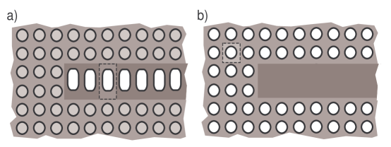
Figure 1: a) Domain $\Omega$ (grey) including the open $\mathsf{I}$-shaped waveguide $\Omega^{1+}$ (dark grey). b) Strip $\varpi^{+}$ (dark grey), which coincides with the open waveguide $\Omega^{1+}$ in the special case $\vartheta^{1}=\varnothing$. Dotted lines indicate in a) the cell $\omega^{1}$ and in b) the cell $\omega^{0}$ .

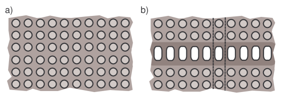
Figure 2: a) Purely periodic plane $\Omega^{0}$. b) Plane $\Omega^{\sharp}$ with infinite perforated strip $\Omega^{1}$ (dark grey) and the strip $\Pi$ (between dotted lines).

1.2 Purely periodic medium.

We consider the geometry of the unperturbed perforated plane and the related spectral boundary value problem. Let $\mathbf{Q}=\mathbf{Q}_{1}\subset{\mathbb{R}}^{2}$ be the unit open square, $\mathbf{Q}_{a}=\left(0,a\right)\times\left(0,a\right),$ and let $\vartheta^{0}$ be an open set in the plane $\mathbb{R}^{2}$ with closure $\overline{\vartheta^{0}}=\vartheta^{0}\cup\partial\vartheta^{0}\subset\mathbf{Q}$ and a smooth boundary $\partial\vartheta$ of Hölder class $C^{2,\delta}$, where $\delta>0$. Here $\vartheta^{0}$ is a not necessarily connected set describing perforation; neither the case $\vartheta^{0}=\emptyset$ is excluded. We define the periodicity cells (outlined by dotted line in Fig. 1, b)

$$\omega^{0}\left(\alpha\right)=\left\{x=\left(x_{1},x_{2}\right):\left(x_{1}-\alpha_{1},x_{2}-\alpha_{2}\right)\in\omega^{0}:=\mathbf{Q}\setminus\overline{\vartheta^{0}}\right\}$$ (1.1)

where $\alpha=\left(\alpha_{1},\alpha_{2}\right)\in\mathbb{Z}^{2}$ is a multi-index and $\mathbb{Z}=\left\{0,\pm 1,\pm 2,...\right\}.$ The perforated plane $\Omega^{0}$ is covered by the periodicity cells (1.1), so it satisfies

$$\overline{\Omega^{0}}={\displaystyle\bigcup_{\alpha\in\mathbb{Z}^{2}}}\overline{\omega^{0}\left(\alpha\right)},\ \ \ \ \Omega^{0}=\mathbb{R}^{2}\setminus{\displaystyle\bigcup_{\alpha\in\mathbb{Z}^{2}}}\overline{\vartheta^{0}\left(\alpha\right)},$$ (1.2)

where $\vartheta^{0}\left(\alpha\right)$ denotes a translation of $\vartheta^{0}$ similarly to (1.1). Assuming $\omega^{0}$ to be a domain, we observe that $\omega^{0}$ includes the boundary strip

$$\left\{x\in\mathbf{Q}\,:\,\mbox{dist}\left(x,\partial\mathbf{Q}\right)<d\right\}$$ (1.3)

with some $d>0$ and, thus, $\Omega^{0}$ is a domain and in particular a connected set as well.

We consider the spectral problem

$$L^{0}\left(x,\nabla\right)u^{0}\left(x\right) =\lambda u^{0}\left(x\right),\ \ \ x\in\Omega^{0},$$ (1.4)

$$N^{0}\left(x,\nabla\right)u^{0}\left(x\right) =0,\ \ \ x\in\partial\Omega^{0},$$ (1.5)

and its variational form

$$\left(A^{0}D\left(\nabla\right)u^{0},D\left(\nabla\right)v^{0}\right)_{\Omega^{0}}=\lambda\left(u^{0},v^{0}\right)_{\Omega^{0}},\ \ \ \forall v^{0}\in H^{1}\left(\Omega^{0}\right)^{n}.$$ (1.6)

Concerning the notation, by $\lambda$ we understand a spectral parameter and $u=\left(u_{1},...,u_{n}\right)^{\top}$ is a vector function, realized as a column, so that $\top$ stands for transposition. The matrix differential operators $L^{0}$ and $N^{0}$ in (1.4) and (1.5) take the form

$$L^{0}\left(x,\nabla\right) =\overline{D\left(-\nabla\right)}^{\top}A^{0}\left(x\right)D\left(\nabla\right),$$ (1.7)

$$N^{0}\left(x,\nabla\right) =\overline{D\left(\nu\left(x\right)\right)}^{\top}A^{0}\left(x\right)D\left(\nabla\right),$$ (1.8)

while $\nabla=\operatorname{grad},$ $\nu=\left(\nu^{1},\nu^{2}\right)^{\top}$ is the unit outward normal vector on $\partial\Omega^{0}$ and $A^{0}$ is a matrix function of size $m\times m$ with $C^{1,\delta}$-smooth entries; $A^{0}\left(x\right)$ is Hermitian, positive definite and 1-periodic in $x\in\mathbb{R}^{2}$ (it is convenient to define the coefficient matrix in the intact plane). Furthermore, $D\left(x\right)$ is a matrix function of size $m\times n$ and linear in $x=(x_{1},x_{2})$, and $D(0,0)=\mathbb{O}_{n\times m}$ is the null matrix. The substitution $x_{j}\mapsto\partial/\partial x_{j}$ gives an $m\times n$-matrix $D\left(\nabla\right)$ of first order differential operators with constant complex coefficients, while $L^{0}(x,\nabla)$ (respectively, $N^{0}(x,\nabla)$) is a formally self-adjoint differential matrix operator in divergence form (resp. the corresponding Neumann condition operator); the bar in (1.7) and (1.8) indicates complex conjugation. Finally, $\left(\ ,\ \right)_{\Omega^{0}}$ is the natural scalar product in the Lebesgue space $L^{2}\left(\Omega^{0}\right)$, and $H^{1}\left(\Omega^{0}\right)$ is the Sobolev space with standard norm

$$\left\|w;H^{1}\left(\Omega^{0}\right)\right\|=\left(\left\|\nabla w;L^{2}\left(\Omega^{0}\right)\right\|^{2}+\left\|w;L^{2}\left(\Omega^{0}\right)\right\|^{2}\right)^{1/2}.$$

The last superscript $n$ in the integral identity (1.6) shows the number of components in the test function $v=\left(v_{1},...,v_{n}\right)^{\top},$ however, this index is omitted in the notation of norms and scalar products. In this way, the left- and right-hand sides of (1.6) involve scalar products in $L^{2}\left(\Omega^{0}\right)^{m}$ and $L^{2}\left(\Omega^{0}\right)^{n}$, respectively.

We assume that $D\left(x\right)$ is algebraically complete [40]: there exists a $\varrho_{D}\in\mathbb{N}=\left\{1,2,3,...\right\}$ such that for any row $p=\left(p_{1},...,p_{n}\right)$ of homogeneous polynomials in $\xi=\left(\xi_{1},\xi_{2}\right)\in\mathbb{R}^{2}$ of common degree $\varrho\geq\varrho_{D},$ one can find a row of polynomials $q=\left(q_{1},...,q_{n}\right)$ satisfying

$$p\left(\xi\right)=q\left(\xi\right)D\left(\xi\right),\ \ \ \ \forall\xi\in\mathbb{R}^{2}.$$ (1.9)

According to [40, § 3.7.4], this assumption yields the Korn inequality

$$\left\|u;H^{1}\left(\Omega^{0}\right)\right\|^{2}\leq c_{D,\omega^{0}}\left(\left\|D\left(\nabla\right)u;L^{2}\left(\omega^{0}\right)\right\|^{2}+\left\|u;L^{2}\left(\omega^{0}\right)\right\|^{2}\right)$$ (1.10)

and, hence, the sesquilinear Hermitian positive form $a^{0}\left(u^{0},v^{0}\right)$ on the left in (1.6) is closed in $H^{1}\left(\Omega^{0}\right)^{n}.$ Moreover, the operator $L^{0}$ is elliptic and the Neumann boundary operator $N^{0}$ covers it in the Shapiro-Lopatinskii sense everywhere on $\partial\Omega^{0}$ (see, e.g., [35, Thm. 1.9]).

Owing to the above-mentioned properties of $a^{0}$, the problem (1.4), (1.5) is associated with a positive self-adjoint operator $\mathcal{A}^{0}$ in $L^{2}\left(\Omega^{0}\right)^{n}$ with the differential expression $L^{0}\left(x,\nabla\right)$ and the domain

$$\mathcal{D}\left(\mathcal{A}^{0}\right)=\left\{u^{0}\in H^{2}\left(\Omega^{0}\right):N^{0}\left(x,\nabla\right)u^{0}\left(x\right)=0,\ x\in\partial\Omega^{0}\right\};$$ (1.11)

see [4, Ch. 10] and [44, Ch. 13]. The description of the spectrum $\sigma\left(\mathcal{A}^{0}\right)$ is well known and will be presented in Section 2.

We emphasize that the results of the paper remain valid for other types of boundary conditions, in particular, for the Dirichlet conditions, cf. Section 4.1.$(i)$,$(iv)$. A description of all admissible boundary conditions can be found in [31] and [35, § 1]. Moreover, the $C^{2,\delta}$-smoothness of the boundary was assumed in order to have the elementary formula (1.11) for the operator domain $\mathcal{D}\left(\mathcal{A}^{0}\right)$ and to simplify the technical computations. The results of our paper hold true in the case of uniformly Lipschitz boundaries, but the proofs would require small modifications, cf. Section 4.2.

1.3 Periodic medium with open semi-infinite periodic waveguide.

In this section we describe the geometry of the open waveguide and the full spectral problem. Let $\varpi^{+}$ be the semi-strip $\left\{x:x_{1}>0,\ \left|x_{2}\right|<h\right\}$ with some $h\in\mathbb{N}$ (overshaded in Fig. 1, b). In the rectangle $\mathbf{Q}_{1}^{h}=\left(0,1\right)\times\left(-h,h\right),$ we introduce an open set $\vartheta^{1}$ with a smooth boundary $\partial\vartheta^{1}$ and closure $\overline{\vartheta^{1}}\subset\mathbf{Q}_{1}^{h}.$ We define a semi-infinite row of holes or inclusions as depicted in Fig. 1, a) or b), respectively:

$$\omega^{1}\left(\alpha_{1}\right) =\left\{x:\left(x_{1}-\alpha_{1},x_{2}\right)\in\omega^{1}\right\},\ \ \alpha_{1}\in\mathbb{N}_{0}=\mathbb{N\cup}\left\{0\right\},$$ (1.12)

$$\omega^{1} =\mathbf{Q}_{1}^{h}\setminus\overline{\vartheta^{1}},\ \ \vartheta^{1}\left(\alpha_{1}\right)=\left\{x:\left(x_{1}-\alpha_{1},x_{2}\right)\in\vartheta^{1}\right\}.$$

The cell $\omega^{1}$ is outlined in Fig. 1, a), by dotted line. We also introduce a smooth Hermitian matrix function $A^{1+}$ in $\mathbb{R}^{2},$ entries of which are supported in $\varpi^{+}$ and become $1$-periodic in $x_{1}$ inside the semi-strip $\left\{x\in\varpi^{+}:x_{1}>R\right\},$ $R\in\mathbb{N}$,

$$A^{1+}\left(x\right)=A^{1}\left(x\right)\text{ \ for \ }x_{1}>R,\ \ \ A^{1}\left(x_{1}\pm 1,x_{2}\right)=A^{1}\left(x_{1},x_{2}\right).$$ (1.13)

Furthermore,

$$\Omega^{1+}=\varpi^{+}\setminus{\displaystyle\bigcup_{\alpha_{1}\in\mathbb{N}_{0}}}\overline{\vartheta^{1}\left(\alpha_{1}\right)},\ \ \ \overline{\Omega^{1+}}={\displaystyle\bigcup_{\alpha_{1}\in\mathbb{N}_{0}}}\overline{\omega^{1}\left(\alpha_{1}\right)},$$ (1.14)

and the sum

$$A\left(x\right)=A^{0}\left(x\right)+A^{1+}\left(x\right)$$ (1.15)

is assumed to be positive definite in $\overline{\Omega}$, where

$$\Omega=\left(\Omega^{0}\setminus\varpi^{+}\right)\cup\Omega^{1+}.$$ (1.16)

In other words, we make a perturbation of coefficients and boundary inside the semi-strip $\varpi^{+}$, see Fig. 1. For instance, one may suppose that $A^{1+}$ is the null matrix $\mathbb{O}_{m\times m}$ and $\vartheta^{0}\neq\varnothing,$ $\vartheta^{1}=\varnothing,$ $h=1,$ which means filling in all holes inside $\varpi^{+},$ cf. Fig. 1, b). Vice versa, in the case $\vartheta^{0}=\varnothing,$ $\vartheta^{1}\neq\varnothing,$ one perforates the plane $\mathbb{R}^{2}$ with a semi-infinite row of holes, see Fig. 1, a). Even in the case of absence of holes we still call (1.14) the perforated strip, and the perforated plane $\Omega^{0}$ in (1.2) can also contain no holes.

Notice that the Korn inequality

$$\left\|u;H^{1}\left(\Omega\right)\right\|^{2}\leq c_{D}\left(\omega^{0},\omega^{1}\right)\left(\left\|D\left(\nabla\right)u;L^{2}\left(\Omega\right)\right\|^{2}+\left\|u;L^{2}\left(\Omega\right)\right\|^{2}\right)$$ (1.17)

is still valid and can be derived by summing up inequalities of type (1.10) in the cells $\omega^{0}\left(\alpha\right)$ with $\alpha\in\mathbb{Z}^{2}$ ($\alpha_{1}>0,$ $-h\leq\alpha_{2}<h$ excluded) and $\omega^{1}\left(\alpha_{1}\right)$ with $\alpha_{1}\in\mathbb{N}_{0}.$

Replacing $A^{0}\left(x\right)$ with (1.15) in (1.7) still gives an elliptic and formally self-adjoint matrix operator $L\left(x,\nabla_{x}\right).$ The same change in (1.8) yields the Neumann boundary condition operator $N\left(x,\nabla_{x}\right),$ where $\nu$ is regarded as the outward unit normal on $\partial\Omega$. In the domain (1.16) we consider the spectral problem

$$L\left(x,\nabla\right)u\left(x\right) =\lambda u\left(x\right),\ \ \ x\in\Omega,$$ (1.18)

$$N\left(x,\nabla\right)u\left(x\right) =0,\ \ \ x\in\partial\Omega,$$ (1.19)

and the corresponding integral identity

$$a\left(u,v\right):=\left(AD\left(\nabla\right)u,D\left(\nabla\right)v\right)_{\Omega}=\lambda\left(u,v\right)_{\Omega},\ \ \ \forall v\in H^{1}\left(\Omega\right)^{n}.$$ (1.20)

Since $a$ remains as a closed positive Hermitian form in $H^{1}\left(\Omega\right)^{n},$ the variational formulation (1.20) of the problem (1.18), (1.19) supplies it with a positive self-adjoint operator $\mathcal{A}$ in $L^{2}\left(\Omega\right)^{n}$ with the differential expression $L\left(x,\nabla\right)$ and the domain

$$\mathcal{D}\left(\mathcal{A}\right)=\left\{u\in H^{2}\left(\Omega^{0}\right)^{n}:N\left(x,\nabla\right)u\left(x\right)=0,\ x\in\partial\Omega\right\};$$ (1.21)

see again [4, Ch. 10] and [44, Ch. 13]. This notation is quite similar to the one used in Section 1.2.

The main goal of the paper is to describe the essential component $\sigma_{es}\left(\mathcal{A}\right)$ in the spectrum of $\mathcal{A}$,

$$\sigma\left(\mathcal{A}\right)=\sigma_{di}\left(\mathcal{A}\right)\cup\sigma_{es}\left(\mathcal{A}\right).$$ (1.22)

We emphasize that in general

$$\sigma_{es}\left(\mathcal{A}\right)\neq\sigma_{es}\left(\mathcal{A}^{0}\right),$$ (1.23)

and moreover, the discrete spectrum of $\mathcal{A}^{0}$ is empty, thus,

$$\sigma_{es}\left(\mathcal{A}^{0}\right)=\sigma\left(\mathcal{A}^{0}\right).$$ (1.24)

We will identify the difference

$$\sigma_{ad}\left(\mathcal{A}\right)=\sigma_{es}\left(\mathcal{A}\right)\setminus\sigma\left(\mathcal{A}^{0}\right),$$ (1.25)

but leave aside two interesting and important questions. First, we are not able to describe completely the component $\sigma_{di}\left(\mathcal{A}\right)$ in a general perturbed problem (1.18), (1.19), although, of course concrete examples of isolated and embedded eigenvalues in $\sigma_{po}\left(\mathcal{A}\right)$ can be constructed in scalar problems. Second, the existence or absence of the point spectrum $\sigma_{po}\left(\mathcal{A}^{0}\right)$ (eigenvalues of infinite multiplicity) in the purely periodic problem (1.4), (1.5) remains unknown; note that this question is answered in the literature only for particular scalar problems (see, e.g., papers [46, 18, 24] and books [43, 28]). Notice that $\sigma_{po}\left(\mathcal{A}^{0}\right)$ can be included in $\sigma_{po}\left(\mathcal{A}\right)$, but the latter stays unknown, too.

1.4 Discussion on the main result

In the case of the purely periodic plane $\Omega^{0}$, Fig. 2, a), the spectrum $\sigma_{es}\left(\mathcal{A}^{0}\right)$ of the problem (1.4)-(1.5) has representation as a union of spectral bands (see (2.15), (2.16), below), which is a well-known consequence of the FBG-theory; we refer here to [27, 28, 45]. Consider for a moment the domain $\Omega^{\sharp}$ of Fig. 2, b) with foreign inclusions or holes, which form a periodic row, infinite in both directions. Then, the spectrum may be different from the purely periodic case, and we denote by $\sigma^{\sharp}$ the essential spectrum of the problem on $\Omega^{\sharp}$ (cf. (3.4), below). Analogously to [17, 21, 22], the increment $\sigma^{\sharp}\setminus\sigma_{es}\left(\mathcal{A}^{0}\right)$ can be detected by performing the partial FBG-transform in $x_{1}$-direction (Section 3.1) and investigating the kernel of the model problem in the perforated strip $\Pi$ (separated by dashed lines in Fig. 2, b); cf. (3.11), (3.9) ). This problem depends on the Floquet parameter $\zeta$, and, for certain values of the spectral parameter $\lambda\in\left(0,+\infty\right)$ and $\zeta\in\left[0,2\pi\right),$ it can have a solution in the Sobolev space $H^{2}(\Pi)^{n}.$ Such values $\lambda$ form the point spectrum $\sigma_{po}\left(\mathcal{A}^{\sharp}\left(\zeta\right)\right)$ of the model problem (3.30) for the operator $\mathcal{A}^{\sharp}\left(\zeta\right)$.

Our main result in Theorem 7 says that the following formula holds true for the problem (1.18), (1.19) in the periodic plane with the immersed $\mathsf{I}$-shaped open waveguide, see (1.16) and Fig. 1, b):

$$\sigma_{ad}\left(\mathcal{A}\right)=\sigma^{\sharp}\setminus\sigma_{es}\left(\mathcal{A}^{0}\right)={\displaystyle\bigcup_{\zeta\in\left[0,2\pi\right)}}\sigma_{po}\left(\mathcal{A}^{\sharp}\left(\zeta\right)\right)\setminus\sigma_{es}\left(\mathcal{A}^{0}\right).$$ (1.26)

The last set in this formula requires some comments. First, embedded eigenvalues in $\sigma_{em}\left(\mathcal{A}^{\sharp}\left(\zeta\right)\right)=\sigma_{po}\left(\mathcal{A}^{\sharp}\left(\zeta\right)\right)\setminus\sigma_{di}\left(\mathcal{A}^{\sharp}\left(\zeta\right)\right)$ live inside the essential spectrum $\sigma_{es}\left(\mathcal{A}^{\sharp}\left(\zeta\right)\right)$, which in turn is contained in $\sigma_{es}\left(\mathcal{A}^{0}\right)$ (compare (3.32) with (2.15)). Second, $\sigma_{es}\left(\mathcal{A}^{\sharp}\left(\zeta\right)\right)$ depends on $\zeta$ and therefore some points of the discrete spectrum $\sigma_{di}\left(\mathcal{A}^{\sharp}\left(\zeta\right)\right)$ may fall into $\sigma_{es}\left(\mathcal{A}^{\sharp}\left(\zeta^{\prime}\right)\right)$ with $\zeta^{\prime}\neq\zeta.$ In any case none of the indicated points in $\sigma_{po}\left(\mathcal{A}^{\sharp}\left(\zeta\right)\right)$ stays in the increment component (1.25) of $\sigma_{es}\left(\mathcal{A}\right).$

We emphasize that, contrary to the case of $\Omega^{\sharp}$, the lacking periodicity of the domain $\Omega$ prevents a direct use of the partial FBG-transform, hence, the proof of (1.26) requires improved mathematical tools. The new procedure of our paper involves the construction of a parametrix and singular Weyl sequences in order to describe, respectively, the regularity field and the essential spectrum of the operator $\mathcal{A}$.

1.5 Cranked and branching open waveguides

Fig. 3 shows open waveguides of the shape of the letters $\mathsf{V},$ $\mathsf{X}$ and $\mathsf{Y},$ $\mathsf{Z}.$ They appear due to perforation and perturbation of coefficients in overshadowed joints of semi-strips. In Section 4 we explain how the results of Section 3 for the $\mathsf{I}$-shaped case, Fig. 1, a), b), can be readily adapted to these cranked and branching open waveguides. Here, skewed branches of the $\mathsf{V}$- and $\mathsf{Y}$-shaped waveguides must maintain the periodicity and thus the tangent of tilt angles has to be rational number. We do not know a formula for the essential spectrum in the irrational case.

We also emphasize that for a clear reason, no relevant perturbation in a disk $\mathbb{B}_{R}=\left\{x:r=\left|x\right|<R\right\}$ with radius $R>0$ can affect the essential spectrum of the boundary value problem (1.18), (1.19). Moreover, assume that $\widetilde{A}\left(x\right)$ is a matrix decaying together with its derivatives at infinity as $\left(1+\left|x\right|\right)^{-\delta},$ $\delta>0$, and that the coefficient matrix (1.15)

$$A\left(x\right)+\widetilde{A}\left(x\right)$$ (1.27)

still keeps the above mentioned basic properties of $A$. This replacement of the coefficient matrix does not change $\sigma_{es}$.

All these generalizations and some others will be commented in Section 4. We have chosen the very particular open waveguide in Section 1.3 in order to simplify the presentation, to illuminate the main points of our approach and to avoid unimportant but cumbersome technical details.

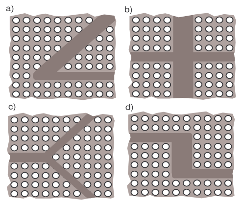
Figure 3: $\mathsf{V,X}$ and $\mathsf{Y,Z}$-shaped joints of open waveguides (dark grey).

1.6 Structure of the paper

In Section 2 we recall generally known information on the purely periodic case which will be used later on. The main interest is focused on the model problem (2.11) in the periodicity cell $\varpi$, which is obtained using the FBG-transform [19]. The open periodic semi-infinite waveguide will be considered in Section 3, where we apply the partial $(FGB)$-transform to formulate another model problem (3.30) in the perforated infinite strip $\Pi$ with periodicity conditions on its lateral sides.

The spectra of those two model problems form the essential spectrum $\sigma_{es}\left(\mathcal{A}\right)$ of the original problem (1.20). To verify the corresponding formulas (3.38) and (2.16), (3.39) we first present two types of singular Weyl sequences for $\mathcal{A}$ and on the other hand construct a right parametrix for the formally self-adjoint problem (1.18), (1.19). This is the most involved part of our paper. To that end, we follow [33] and also [39, §3.4], and study an operator family for a second model problem in the weighted Sobolev spaces (Kondratiev spaces) $W_{\beta}^{l}\left(\Pi\right),$ leading to important conclusions on exponential decay properties of the solutions in the strip $\Pi.$ Finally, we glue the parametrix (3.46) from solutions of the model problems with the help of appropriate cut-off functions. The parametrix enables to prove that, for any $\lambda\in\overline{\mathbb{R}_{+}}$ outside the union of sets (2.16) and (3.39), the operator of the inhomogeneous problem (1.18), (1.19), cf. (3.40), is Fredholm in the Sobolev-Slobodetskii spaces; therefore such points $\lambda$ form the intersection of the regularity field of ${\mathcal{A}}$ with the semi-axis $\overline{\mathbb{R}_{+}}.$ This completes the proof of Theorem 7, the central assertion in the paper.

We start the last section of the paper by describing several concrete problems in acoustics, elasticity and piezoelectricity, to which our theory may apply. However, as mentioned above, the original exact formulation of the spectral problem was simplified in several aspects, so we comment in the next subsections on certain supplementary issues in order to obtain more generality for further interesting physical applications. We finish the paper with Section 4.5, where we present small modifications of the parametrix to be applied to semi-bounded open periodic waveguides in the shape of the letters $\mathsf{V,X}$ and $\mathsf{Y,Z}$ as in Fig. 3.

2 Spectrum of the purely periodic problem

2.1 Floquet-Bloch-Gelfand-transform

The spectrum of the operator $\mathcal{A}^{0}$ in the purely periodic domain $\Omega^{0}$ can be studied with the help of the FBG-transform. This will lead to the formula (2.16), the main object of Section 2. The FBG-transform is defined by

$$u\mapsto\widehat{u}\left(x;\eta\right)=\frac{1}{2\pi}\sum_{\alpha\in\mathbb{Z}^{2}}e^{-i\eta\cdot\left(x+\alpha\right)}u\left(x+\alpha\right),\ \ \ x\in\omega^{0},$$ (2.1)

and it establishes the isometric isomorphism

$$L^{2}\left(\Omega^{0}\right)\cong L^{2}\left(\mathbf{Y};L^{2}\left(\omega^{0}\right)\right)$$ (2.2)

(cf. [19] and, e.g., [45, 28]), where $\eta\cdot x=\eta_{1}x_{1}+\eta_{2}x_{2},$

$$\mathbf{Y}=\left\{\eta=\left(\eta_{1},\eta_{2}\right):\eta_{1},\eta_{2}\in\left[0,2\pi\right)\right\},\ \ \ \overline{\mathbf{Y}}=\overline{\mathbf{Q}_{2\pi}},$$ (2.3)

and $L^{2}\left(\mathbf{Y};\mathfrak{B}\right)$ is the Lebesgue space of abstract functions in $\eta\in\mathbf{Y}$ with values in Banach space $\mathfrak{B}$ and the norm

$$\left\|U;L^{2}\left(\mathbf{Y};\mathfrak{B}\right)\right\|=\left(\int_{0}^{2\pi}\int_{0}^{2\pi}\left\|U\left(\eta\right);\mathfrak{B}\right\|^{2}d\eta_{1}d\eta_{2}\right)^{1/2}.$$ (2.4)

Moreover, the mapping

$$H^{2}\left(\Omega^{0}\right)^{n}\ni u\mapsto\widehat{u}\in L^{2}\left(\mathbf{Y};H_{\mathrm{per}}^{2}\left(\omega^{0}\right)^{n}\right)$$ (2.5)

is an isomorphism, too. Here, $H_{\mathrm{per}}^{2}\left(\omega^{0}\right)^{n}$ is the subspace of vector functions $U\in H^{2}\left(\omega^{0}\right)^{n}$ satisfying the periodicity conditions

$$U\left(0,x_{2}\right) =U\left(1,x_{2}\right),\ \ \ \frac{\partial U}{\partial x_{1}}\left(0,x_{2}\right)=\frac{\partial U}{\partial x_{1}}\left(1,x_{2}\right),\ \ \ x_{2}\in\left(0,1\right),$$ (2.6)

$$U\left(x_{1},0\right) =U\left(x_{1},1\right),\ \ \ \frac{\partial U}{\partial x_{2}}\left(x_{1},0\right)=\frac{\partial U}{\partial x_{2}}\left(x_{1},1\right),\ \ \ x_{1}\in\left(0,1\right).$$

In what follows we shorten the notation $\partial U/\partial x_{j}$ to $\partial_{j}U.$

The inverse FBG-transform is given by

$$U =\widehat{u}\mapsto u\left(x\right)=\frac{1}{2\pi}\int_{0}^{2\pi}\int_{0}^{2\pi}e^{i\eta\cdot x}U\left(x-\left[x\right];\eta\right)d\eta_{1}d\eta_{2},$$ (2.7)

$$\left[x\right] =\left(\left[x_{1}\right],\left[x_{2}\right]\right),\ \ \ \left[t\right]=\max\left\{\tau\in\mathbb{Z}:\tau\leq t\right\}.$$

2.2 The model problem on the periodicity cell

Owing to (2.1), we have

$$\widehat{\,\,\nabla^{\alpha}v\,\,}\left(x;\eta\right)=\left(\partial_{1}+i\eta\right)^{\alpha_{1}}\left(\partial_{2}+i\eta\right)^{\alpha_{2}}\widehat{v}\left(x;\eta\right),\ \ \ \nabla^{\alpha}=\partial_{1}^{\alpha_{1}}\partial_{2}^{\alpha_{2}}$$ (2.8)

and thus the FBG-transform (2.1) converts the problem (1.4), (1.5) into the following problem, depending on the parameter $\eta\in\mathbf{Y}$, in the periodicity cell $\omega^{0}$ ,

$$L^{0}\left(x,\nabla+i\eta\right)U\left(x;\eta\right) =\Lambda\left(\eta\right)U\left(x;\eta\right),\ \ \ x\in\omega^{0},$$ (2.9)

$$N^{0}\left(x,\nabla+i\eta\right)U\left(x;\eta\right) =0,\ \ \ x\in\gamma^{0}=\partial\omega^{0}\cap\mathbf{Q},$$ (2.10)

together with the periodicity conditions (2.6) on the exterior part $\partial\mathbf{Q}$ of the boundary of the cell $\omega^{0}.$ The variational formulation of problem (2.9), (2.10), (2.6) amounts to finding a number $\Lambda\left(\eta\right)\in\mathbb{C}$ and a non-trivial vector function $U\left(\cdot;\eta\right)\in H_{\mathrm{per}}^{1}\left(\omega^{0}\right)^{n}$ such that

$$\left(A^{0}D\left(\nabla+i\eta\right)U,D\left(\nabla+i\eta\right)V\right)_{\omega^{0}}=\Lambda\left(\eta\right)\left(U,V\right)_{\omega^{0}},\ \ \ \forall V\in H_{\mathrm{per}}^{1}\left(\omega^{0}\right)^{n}.$$ (2.11)

In view of the compact embedding $H^{1}\left(\omega^{0}\right)\subset L^{2}\left(\omega^{0}\right)$ in the bounded domain $\omega^{0},$ the spectrum $\sigma_{\eta}^{0}$ of the variational problem (2.11) and boundary value problem (2.9), (2.10), (2.6) is discrete and forms the unbounded monotone sequence

$$0\leq\Lambda_{1}\left(\eta\right)\leq\Lambda_{2}\left(\eta\right)\leq...\leq\Lambda_{k}\left(\eta\right)\leq...\rightarrow+\infty,$$ (2.12)

where multiplicities are counted. According to the general results of the perturbation theory for linear operators, the functions

$$\mathbf{Y}\ni\eta\mapsto\Lambda_{k}\left(\eta\right)$$ (2.13)

are continuous, see for example [23, 25]. Moreover, they are $2\pi$-periodic in $\eta_{1}$ and $\eta_{2}$, because for any eigenpair $\left\{\Lambda\left(\eta\right),U\left(x;\eta\right)\right\}$ of the problem (2.9), (2.10), (2.6) at some $\eta\in\mathbf{Y},$

$$\left\{\Lambda\left(\eta\right),e^{\pm 2\pi ix_{p}}U\left(x;\eta\right)\right\},\ p=1,2,$$ (2.14)

remains an eigenpair of the same problem but at $\eta\pm 2\pi e_{\left(p\right)}$ where $e_{\left(p\right)}=\left(\delta_{1,p},\delta_{2,p}\right)^{\top}\in\mathbb{R}^{2}$ is the unit vector of the $\eta_{p}$-axis.

The above mentioned properties of functions (2.13) ensure that the spectral bands

$$B_{k}^{0}=\left\{\Lambda_{k}\left(\eta\right):\eta\in\mathbf{Y}\right\},\ k\in\mathbb{N},$$ (2.15)

are bounded connected closed segments in $\overline{\mathbb{R}_{+}}.$ The formula

$$\sigma\left(\mathcal{A}^{0}\right)=\sigma_{es}\left(\mathcal{A}^{0}\right)={\displaystyle\bigcup_{k\in\mathbb{N}}}B_{k}^{0}$$ (2.16)

for the spectrum of the problem (1.4), (1.5) is well-known, see, e.g., [27, 45, 28], but we briefly comment on its proof in Sections 2.3–2.4, since we will need some of these arguments later.

2.3 Unique solution of the inhomogeneous problem

As regards to (2.16), we now prove the inclusion $\sigma\left(\mathcal{A}^{0}\right)\subset\cup_{k\in\mathbb{N}}B_{k}^{0}$. Let us consider the boundary value problem

$$L^{0}\left(x,\nabla\right)u^{0}\left(x\right)-\lambda u^{0}\left(x\right) =f^{0}\left(x\right),\ \ \ x\in\Omega^{0},$$ (2.17)

$$N^{0}\left(x,\nabla\right)u^{0}\left(x\right) =g^{0}\left(x\right),\ \ \ x\in\partial\Omega^{0},$$

with the data

$$f^{0}\in L^{2}\left(\Omega^{0}\right)^{n},\ g^{0}\in H^{1/2}\left(\partial\Omega^{0}\right)^{n}$$ (2.18)

and a fixed parameter $\lambda=\lambda^{0}$ such that

$$\lambda^{0}\notin B_{k}^{0},\ \ \forall k\in\mathbb{N}.$$ (2.19)

In (2.18), $H^{1/2}\left(\partial\Omega^{0}\right)$ stands for the Sobolev-Slobodetskii space of traces with the intrinsic norm

$$\left\|g^{0};H^{1/2}\left(\partial\Omega^{0}\right)\right\|=\inf\left\{\left\|G^{0};H^{1}\left(\Omega^{0}\right)\right\|:G^{0}=g^{0}\text{ on }\partial\Omega^{0}\right\}.$$ (2.20)

This norm is equivalent to the following one:

$$\left(\left\|g^{0};L^{2}\left(\partial\Omega^{0}\right)\right\|^{2}+\int_{\partial\Omega^{0}}\int_{\partial\Omega_{l}^{0}\left(x\right)}\left|g^{0}\left(x\right)-g^{0}\left(y\right)\right|^{2}\frac{ds_{x}ds_{y}}{\left|x-y\right|^{2}}\right)^{1/2}.$$

Here, $ds_{x}$ is the arc length element on $\partial\Omega^{0}$ and $\partial\Omega_{l}^{0}\left(x\right)=\left\{y\in\partial\Omega^{0}:\left|y-x\right|<l\right\}$ while $l\in\left(0,+\infty\right)$ can be fixed arbitrarily.

Clearly, the mapping

$$H^{2}\left(\Omega^{0}\right)^{n}\ni u\mapsto\left\{L^{0}u^{0}-\lambda^{0}u^{0},N^{0}u^{0}\right\}\in L^{2}\left(\Omega^{0}\right)^{n}\times H^{1/2}\left(\partial\Omega^{0}\right)^{n}$$ (2.21)

is continuous for any $\lambda^{0}$, but in the case (2.19) it becomes an isomorphism. Indeed, the FBG-transform (2.1) turns (2.17) into the parameter-dependent problem

$$L^{0}\left(x,\nabla+i\eta\right){\widehat{u}\,}^{0}\left(x;\eta\right)-\lambda^{0}{\widehat{u}\,}^{0}\left(x;\eta\right) ={\widehat{f}\ }^{0}\left(x;\eta\right),\ \ \ x\in\omega^{0},$$ (2.22)

$$N^{0}\left(x,\nabla+i\eta\right){\widehat{u}\,}^{0}\left(x;\eta\right) ={\widehat{g}\;}^{0}\left(x;\eta\right),\ \ \ x\in\gamma^{0},$$

with the periodicity conditions (2.6). The right-hand sides meet the estimate

$$\left\|{\widehat{f}\ }^{0};L^{2}\left(0,2\pi;L^{2}\left(\omega^{0}\right)\right)\right\|^{2}+\left\|{\widehat{g}\;}^{0};L^{2}\left(0,2\pi;H^{1/2}\left(\gamma^{0}\right)\right)\right\|^{2}$$ (2.23)

$$\leq c\left(\left\|f^{0};L^{2}\left(\Omega^{0}\right)\right\|^{2}+\left\|g^{0};H^{1/2}\left(\partial\Omega^{0}\right)\right\|^{2}\right),$$

while the necessary information about the Sobolev-Slobodetskii space is provided by the isomorphisms (2.2), (2.4) and the formula (2.8) for derivatives. By the assumption (2.19), the problem (2.22), (2.6) has for any $\eta\in\mathbf{Y}$ a unique solution denoted by

$${\widehat{u}\,}^{0}\left(x;\eta\right)=R^{0}\left(\lambda^{0};\eta\right)\left\{{\widehat{f}\ }^{0}\left(\cdot;\eta\right),{\widehat{g}\;}^{0}\left(\cdot;\eta\right)\right\}$$ (2.24)

and estimated as follows:

$$\left\|{\widehat{u}\,}^{0}\left(\cdot;\eta\right);H^{2}\left(\omega^{0}\right)\right\|^{2}\leq C\left(\left\|{\widehat{f}\ }^{0}\left(\cdot;\eta\right);L^{2}\left(\omega^{0}\right)\right\|^{2}+\left\|{\widehat{g}\;}^{0}\left(\cdot;\eta\right);H^{1/2}\left(\gamma^{0}\right)\right\|^{2}\right).$$ (2.25)

Since the constant $C$ does not depend on $\eta\in\mathbf{Y}$, it suffices to apply the inverse FBG-transform (2.7) and to derive from (2.25) and (2.23) the inequality

$$\left\|u^{0};H^{2}\left(\Omega^{0}\right)\right\|^{2}\leq c\left(\left\|f^{0};L^{2}\left(\Omega^{0}\right)\right\|^{2}+\left\|g^{0};H^{1/2}\left(\partial\Omega^{0}\right)\right\|^{2}\right)$$ (2.26)

for the unique solution $u^{0}\in H^{2}\left(\Omega^{0}\right)^{n}$ of the problem (2.17) with fixed parameter (2.19). Thus, mapping (2.21) with this $\lambda^{0}$ is indeed an isomorphism, which in particular means that $\lambda^{0}$ belongs to the regularity field of the operator $\mathcal{A}^{0}$ in (1.11). This coincides with the resolvent set of $\mathcal{A}^{0}$ because the discrete spectrum $\sigma_{di}\left(\mathcal{A}^{0}\right)$ is evidently empty.

Remark 1

Dealing with the Sobolev-Slobodetskii norms in (2.23), (2.25) and (2.26), it is much more convenient to use the definition (2.20) and some extensions $G$ of $g$ and $\widehat{G}\left(\cdot;\eta\right)$ of $\widehat{g}\left(\cdot;\eta\right)$ such that

$$\left\|g;H^{1/2}\left(\partial\Omega^{0}\right)\right\| \leq 2\left\|G;H^{1}\left(\Omega^{0}\right)\right\|\text{,}$$

$$\left\|\widehat{g};L^{2}\left(0,2\pi;H^{1/2}\left(\gamma^{0}\right)\right)\right\| \leq 2\left\|\widehat{G};L^{2}\left(0,2\pi;H^{1/2}\left(\gamma^{0}\right)\right)\right\|.\ \ \blacksquare$$

2.4 The singular Weyl sequence

We next show that $\sigma\left(\mathcal{A}^{0}\right)\supset\cup_{k\in\mathbb{N}}B_{k}^{0}$. Let us assume

$$\lambda^{0}\in B_{k}^{0}\ \text{for some }k\in\mathbb{N}$$ (2.27)

so that there exist $\eta^{0}\in\mathbf{Y}$ and $U^{0}\left(\cdot;\eta^{0}\right)\in H^{2}\left(\omega^{0}\right)$ such that $\left\{\eta^{0},U^{0}\left(\cdot;\eta^{0}\right)\right\}$ is an eigenpair of the problem (2.9), (2.10), (2.6) with $\Lambda\left(\eta^{0}\right)=\lambda^{0}$. By a direct calculation, one easily deduces that the Bloch wave

$$u^{0}\left(x\right)=e^{i\eta^{0}\cdot x}U^{0}\left(x;\eta^{0}\right)$$ (2.28)

satisfies the differential equations (1.4) and the boundary conditions (1.5), although it does of course not fall into the Sobolev space $H^{2}\left(\Omega^{0}\right)^{n}.$ However, (2.28) is useful for constructing a singular sequence $\left\{u^{0j}\right\}_{j\in\mathbb{N}}$ in $\mathcal{D}\left(\mathcal{A}^{0}\right)\subset H^{2}\left(\Omega^{0}\right)^{n}$ for the operator $\mathcal{A}^{0}$ at the point $\lambda^{0},$ namely a sequence with the following properties:

1${}^{\text{o}}$  $\left\|u^{0j};L^{2}\left(\Omega^{0}\right)\right\|=1;$

2${}^{\text{o}}$  $u^{0j}\rightharpoondown 0$ weakly in $L^{2}\left(\Omega^{0}\right)^{n}$ as $j\rightarrow+\infty;$

3${}^{\text{o}}$  $\left\|\mathcal{A}^{0}u^{0j}-\lambda^{0}u^{0j};L^{2}\left(\Omega^{0}\right)\right\|\rightarrow 0$ as $j\rightarrow+\infty.$

To define the entries of this sequence, we introduce the plateau function

$$\chi_{j}\left(t\right)=\chi\left(t-2^{j}\right)\chi\left(2^{j+1}-t\right),$$ (2.29)

where $\chi\in C^{\infty}\left(\mathbb{R}\right)$ is a cut-off function such that

$$\chi\left(t\right)=1\text{ for\ }t\geq d,\ \ \ \ \ \ \chi\left(t\right)=0\text{ \ for \ }t\leq 0,\text{ \ \ \ \ \ }0\leq\chi\leq 1$$ (2.30)

and $d>0$ is taken from (1.3); therefore, in the vicinity of each component $\gamma^{0}\left(\alpha\right)=\partial\vartheta^{0}\left(\alpha\right)$ of the boundary $\partial\Omega^{0}$ the two-dimensional plateau function

$$X_{j}\left(x\right)=\chi_{j}\left(x_{1}\right)\chi_{j}\left(x_{2}\right)$$ (2.31)

becomes a constant, either $1$ or $0.$

We set

$$v^{0j}\left(x\right)=X_{j}\left(x\right)u^{0}\left(x\right),\ \ \ u^{0j}\left(x\right)=\left\|v^{0j};L^{2}\left(\Omega^{0}\right)\right\|^{-1}v^{0j}\left(x\right).$$ (2.32)

The above specification of $X_{j}$ shows that

$$N^{0}\left(x,\nabla\right)v^{0j}\left(x\right)=X_{j}\left(x\right)N^{0}\left(x,\nabla\right)u^{0}\left(x\right)=0,\ \ \ x\in\partial\Omega^{0},$$

and, hence, $u^{0j}\in\mathcal{D}\left(\mathcal{A}^{0}\right).$

The property 1${}^{\text{o}}$ clearly holds true. Furthermore, the weak convergence to $0$ in 2${}^{\text{o}}$ occurs at least along a subsequence of indices $j\in\mathbb{N}$, because, by (2.29) and (2.31), supp$\,\left(v^{0j}\right)\cap\mbox{supp}\left(v^{0l}\right)=\varnothing$ as $j\neq l.$ It remains to verify the property 3${}^{\text{o}}.$ Recalling (2.32) and (2.28), we have

$$\left\|v^{0j};L^{2}\left(\Omega^{0}\right)\right\|^{2} \geq\sum_{\alpha\in\mathbb{Z}^{2}\cap\left[2^{j}+1,2^{j+1}-1\right]}\int_{\omega^{0}\left(\alpha\right)}\left|U^{0}\left(x;\eta^{0}\right)\right|^{2}dx=$$ (2.33)

$$=\left(2^{j+1}-2^{j}-2\right)^{2}\left\|U^{0}\left(\cdot;\eta^{0}\right);L^{2}\left(\omega^{0}\right)\right\|^{2}\geq c_{0}2^{2j}$$

with $c_{0}>0$ and $j\geq 2.$ At the same time, we obtain

$$f^{0j}=L^{0}v^{0j}-\lambda^{0}v^{0j}=\left[L^{0},X_{j}\right]u^{0}+X_{j}\left(L^{0}u^{0}-\lambda^{0}u^{0}\right)=\left[L^{0},X_{j}\right]u^{0}$$

where $\left[L^{0},X_{j}\right]$ stands for the commutator of the differential operator (1.7) and the multiplication operator with $X_{j}.$ Owing to definition (2.29)-(2.31), the plateau function (2.31) varies only inside the union of four rectangles of size $d\times 2^{j}$ and the common area $O\left(2^{j}\right)$ (see the overshaded frame in Fig. 4, a) ). Hence, due to periodicity in (2.28), we arrive at the inequality

$$\left\|f^{0j};L^{2}\left(\Omega^{0}\right)\right\|^{2}\leq c_{1}2^{j},$$

which together with (2.33) and (2.32) prove the relation

$$\left\|\mathcal{A}^{0}u^{0j}-\lambda^{0}u^{0j};L^{2}\left(\Omega^{0}\right)\right\|\leq C2^{-j/2},\ \ C=c_{1}/c_{0}$$

as well as the property 3${}^{\text{o}}$.

By the Weyl criterion (cf. [4, Th. 9.12] or [42, Th. VII.12]), the point (2.27) lives in the essential spectrum $\sigma_{es}\left(\mathcal{A}^{0}\right).$ This and the material of Section 2.3 confirm the formula (2.16).

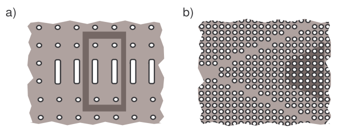
Figure 4: Supports of the cut-off functions.

3 Spectrum of the open waveguide in periodic medium

3.1 Partial Floquet-Bloch-Gelfand-transform

Our aim is to apply the partial FBG-transform to detect the effect of the open waveguide to the essential spectrum of the problem (1.18)–(1.19). Due to the lack of periodicity, this cannot be done directly in $\Omega$, hence, we introduce and study in Sections 3.1–3.3 the problem in the domain $\Omega^{\sharp}$, Fig. 2, b). The results of Section 3.3 will be applied in Sections 3.4–3.5 to the original problem, which leads to the proof of the main result, Theorem 7.

Similarly to (1.14)-(1.16) we introduce the infinite periodically perforated strip $\Omega^{1}$ (overshaded in Fig. 2, b),

$$\Omega^{1}=\varpi\setminus{\displaystyle\bigcup_{\alpha_{1}\in\mathbb{Z}}}\overline{\omega^{1}\left(\alpha_{1}\right)},\ \ \ \ \varpi=\mathbb{R}\times\left(-h,h\right),$$ (3.1)

and the positive definite Hermitian matrix

$$A^{\sharp}\left(x\right)=A^{0}\left(x\right)+A^{1}\left(x\right)$$ (3.2)

which happens to be 1-periodic in the variable $x_{1}.$ In the domain

$$\Omega^{\sharp}=\left(\Omega^{0}\setminus\varpi\right)\cup\Omega^{1}$$ (3.3)

we consider the auxiliary boundary-value problem

$$L^{\sharp}\left(x,\nabla\right)u^{\sharp}\left(x\right)-\lambda^{\sharp}u^{\sharp}\left(x\right) =f^{\sharp}\left(x\right),\ \ \ x\in\Omega^{\sharp},$$ (3.4)

$$N^{\sharp}\left(x,\nabla\right)u^{\sharp}\left(x\right) =g^{\sharp}\left(x\right),\ \ \ x\in\partial\Omega^{\sharp},$$

where $\lambda^{\sharp}$ is a fixed parameter and the operators $L^{\sharp},N^{\sharp}$ are given by (1.7), (1.8) with the change $A^{0}\mapsto A^{\sharp}.$

The domain (3.3) is also 1-periodic along the $x_{1}$-axis, that is

$$\Omega^{\sharp}=\left\{x:\left(x_{1}\pm 1,x_{2}\right)\in\Omega^{\sharp}\right\},$$ (3.5)

and we define the perforated strip bounded by dashed lines in Fig. 2, b),

$$\Pi=\left\{x\in\Omega^{\sharp}:x_{1}\in\left(0,1\right)\right\}.$$ (3.6)

The periodicity observed in (3.2) and (3.3) allows us to apply the partial FBG-transform, see e.g. [33],

$$u^{\sharp}\mapsto U^{\sharp}\left(x;\zeta\right)=\frac{1}{\sqrt{2\pi}}\sum_{\alpha_{1}\in\mathbb{Z}}e^{-i\zeta\left(x_{1}+\alpha_{1}\right)}u^{\sharp}\left(x_{1}+\alpha_{1};x_{2}\right)$$ (3.7)

which establishes the isomorphisms

$$L^{2}\left(\Omega^{\sharp}\right)\simeq L^{2}\left(0,2\pi;L^{2}\left(\Pi\right)\right),\ \ \ H^{2}\left(\Omega^{\sharp}\right)\approx L^{2}\left(0,2\pi;H_{\mathrm{per}\sharp}^{2}\left(\Pi\right)\right)$$ (3.8)

where the first one is isometric (cf. (2.2)), while $H_{\mathrm{per}\sharp}^{2}\left(\Pi\right)^{n}$ is the subspace of functions $U^{\sharp}\in H^{2}\left(\Pi\right)^{n}$ satisfying the periodicity conditions on the lateral sides of the perforated strip (3.6)

$$U^{\sharp}\left(0;x_{2}\right)=U^{\sharp}\left(1;x_{2}\right),\ \ \ \partial_{1}U^{\sharp}\left(0;x_{2}\right)=\partial_{1}U^{\sharp}\left(1;x_{2}\right),\ \ \ x_{2}\in\mathbb{R}.$$ (3.9)

The inverse partial FBG-transform is given by

$$u^{\sharp}\left(x_{1},x_{2}\right)=\frac{1}{\sqrt{2\pi}}\int_{0}^{2\pi}e^{i\zeta x_{1}}U^{\sharp}\left(x_{1}-\left[x_{1}\right],x_{2};\zeta\right)d\zeta,$$ (3.10)

see [33] and cf. (2.1), (2.7).

The FBG-transform (3.7) applies to the problem (3.4) and converts it into the parameter-dependent problem

$$L^{\sharp}\left(x,\partial_{1}+i\zeta,\partial_{2}\right)U^{\sharp}\left(x;\eta\right)-\lambda^{\sharp}U^{\sharp}\left(x;\eta\right) =F^{\sharp}\left(x;\eta\right),\ \ \ x\in\Pi,$$ (3.11)

$$N^{\sharp}\left(x,\partial_{1}+i\zeta,\partial_{2}\right)U^{\sharp}\left(x;\eta\right) =G^{\sharp}\left(x;\eta\right),\ \ \ x\in\Gamma,$$

with the periodicity conditions (3.9). Here, $\lambda^{\sharp}\in\mathbb{R}_{+}$ is fixed, $F^{\sharp},G^{\sharp}$ are the FBG-images of $f^{\sharp},g^{\sharp}$ and

$$\Gamma=\left\{x\in\partial\Pi:0<x_{1}<1\right\}$$ (3.12)

is the interior boundary of the perforated strip $\Pi$.

3.2 Second model problem in weighted spaces

To study the problem (3.11), (3.9), we introduce the weighted Sobolev space $W_{\beta}^{2}\left(\Pi\right)$ (the exponential Kondratiev space [26]) as a completion of the linear set $C_{c}^{\infty}\left(\overline{\Pi}\right)$ (infinitely differentiable functions with compact supports) with respect to the norm

$$\left\|v;W_{\beta}^{2}\left(\Pi\right)\right\|=\left(\left\|\nabla^{2}v;L_{\beta}^{2}\left(\Pi\right)\right\|^{2}+\left\|\nabla v;L_{\beta}^{2}\left(\Pi\right)\right\|^{2}+\left\|v;L_{\beta}^{2}\left(\Pi\right)\right\|^{2}\right)^{1/2},$$ (3.13)

where $\nabla^{2}v$ is the family of all second-order derivatives of $v,$ $\beta\in\mathbb{R}$ is a weight index and $L_{\beta}^{2}\left(\Pi\right)$ stands for the weighted Lebesgue space,

$$\left\|v;L_{\beta}^{2}\left(\Pi\right)\right\|=\left\|e^{\beta\left|x_{2}\right|}v;L^{2}\left(\Pi\right)\right\|.$$ (3.14)

Notice that $W_{\beta}^{2}\left(\Pi\right)$ consists of all functions $v\in H_{loc}^{2}\left(\overline{\Pi}\right)$ with finite norm (3.13). The norm modified by omitting $\left\|\nabla v;L_{\beta}^{2}\left(\Pi\right)\right\|$ on the right in (3.13) remains equivalent to the original one. For $\beta=0,$ we have $W_{0}^{2}\left(\Pi\right)=H^{2}\left(\Pi\right)$, but in the case $\beta>0$ ($\beta<0)$ the Kondratiev space includes functions with an exponential decay (growth) at infinity with decay (growth) rate controlled by the weight index. By $W_{\beta,per\sharp}^{2}\left(\Pi\right),$ we understand the subspace of functions subject to the periodicity conditions (3.9), and $W_{\beta}^{1/2}\left(\Gamma\right)$ is the weighted Sobolev-Slobodetskii space with the intrinsic norm

$$\Big{\|}v;W_{\beta}^{1/2}(\Gamma)\Big{\|} =\inf\Big{\{}\left\|V;W_{\beta}^{1}\left(\Pi\right)\right\|$$

$$=\Big{(}\left\|\nabla V;L_{\beta}^{2}\left(\Pi\right)\right\|^{2}+\left\|V;L_{\beta}^{2}\left(\Pi\right)\right\|^{2}\Big{)}^{1/2}\,:\,V=v\ \mathrm{on}\ \Gamma\Big{\}}.$$ (3.15)

We emphasize that $W_{\beta}^{1/2}\left(\Gamma\right)$ does not require periodicity conditions because (3.12) includes the interior part of the boundary.

Owing to definitions (3.13)-(3.15) and formula (3.8), the partial FBG-transform establishes the isomorphisms

$$L_{\beta}^{2}\left(\Omega^{\sharp}\right) \simeq L^{2}\left(0,2\pi;L_{\beta}^{2}\left(\Pi\right)\right),\ \ \ W_{\beta}^{2}\left(\Omega^{\sharp}\right)\approx L^{2}\left(0,2\pi;W_{\beta,per\sharp}^{2}\left(\Pi\right)\right),$$ (3.16)

$$W_{\beta}^{3/2}\left(\partial\Omega^{\sharp}\right) \approx L^{2}\left(0,2\pi;W_{\beta}^{3/2}\left(\Gamma^{\sharp}\right)\right).$$

The problem operator for (3.11), (3.9) ,

$$W_{\beta,per\sharp}^{2}\left(\Pi\right)^{n} \ni U^{\sharp}\mapsto T_{\beta}^{\sharp}\left(\lambda^{\sharp},\zeta\right)U^{\sharp}$$

$$=\left\{L^{\sharp}\left(x,\partial_{1}+i\zeta,\partial_{2}\right)-\lambda^{\sharp},N^{\sharp}\left(x,\partial_{1}+i\zeta,\partial_{2}\right)\right\}\in L_{\beta}^{2}\left(\Pi\right)^{n}\times W_{\beta}^{1/2}\left(\Gamma\right)^{n}$$ (3.17)

is continuous for any $\beta\in\mathbb{R}$ and $\zeta\in\mathbb{C}$. However, it has better properties under additional assumptions described in terms of the operator pencil

$$\mathbb{C}\ni\eta_{2}\mapsto\mathfrak{A}_{\Lambda}\left(\zeta,\eta_{2}\right)=\left\{L^{0}\left(x,\partial_{1}+i\zeta,\partial_{2}+i\eta_{2}\right)-\Lambda,N^{0}\left(x,\partial_{1}+i\zeta,\partial_{2}+i\eta_{2}\right)\right\}:$$ (3.18)

$$H_{\mathrm{per}}^{2}\left(\omega^{0}\right)^{n}\rightarrow L^{2}\left(\omega^{0}\right)^{n}\times H^{1/2}\left(\gamma^{0}\right)^{n}$$

which corresponds to the problem (2.9), (2.10), (2.6) with the fixed parameter $\Lambda=\lambda^{\sharp}\in\mathbb{R}$ and the dual FBG-variable

$$\eta=\left(\zeta,\eta_{2}\right)\in\mathbf{Y},$$ (3.19)

where $\zeta\in\left[0,2\pi\right)$ is taken from (3.11). Concerning $\eta_{2}$ as a spectral parameter, we regard (3.18) as a quadratic pencil in $\eta_{2},$ which is a particular case of a holomorphic spectral family, see [20, Ch.1].

The following assertion is proved in [33], see also [39, Thms 3.4.7 and 5.1.4].

Theorem 2

The operator (3.17) is Fredholm if and only if the segment

$$\Upsilon_{\beta}=\left\{\eta_{2}\in\mathbb{C}:\operatorname{Re}\eta_{2}\in\left[0,2\pi\right),\ \operatorname{Im}\eta_{2}=\beta\right\}$$ (3.20)

in the complex plane $\mathbb{C}$ is free of the spectrum of the pencil (3.18). If a point of the spectrum belongs to $\Upsilon_{\beta},$ then the range of the operator $T_{\beta}^{\sharp}\left(\lambda^{\sharp},\zeta\right)$ is not closed.

Let us assume that $\lambda^{\sharp}=\lambda^{0}$ satisfies (2.19) and, in particular, that the segment $\Upsilon_{0}$ is free of the spectrum of $\mathfrak{A}_{\lambda^{\sharp}}\left(\zeta,\cdot\right)$ for all $\zeta\in\left[0,2\pi\right).$ Indeed, if $\eta_{2}\in\Upsilon_{0}$ belongs to the spectrum, then $\lambda^{\sharp}=\Lambda\left(\zeta,\eta_{2}\right)$ becomes an eigenvalue of the problem (2.9), (2.10), (2.6) and therefore falls into some spectral band $B_{k}.$ By the analytic Fredholm alternative, see, e.g., [20, Thm. 1.5.1] or [42, Thm. VI.14], we conclude that the spectrum of the pencil (3.18) consists of a countable set of (normal) eigenvalues without finite accumulation points. For $\eta_{2}\in\mathbb{C}$, the spectrum is invariant with respect to the shifts $\eta_{2}\mapsto\eta_{2}\pm 2\pi$ along the real axis, by the same argument as in (2.13) and (2.14). Moreover, it is mirror symmetric with respect to the real axis because, for fixed real $\lambda^{\sharp}$ and $\zeta,$ the problems (2.9), (2.10), (2.6) with $\eta_{2}$ and $\overline{\eta_{2}}$ are formally adjoint. Finally, under the assumption (2.19), there exists a positive continuous $2\pi$-periodic function

$$\left[0,2\pi\right)\ni\zeta\mapsto\beta_{0}\left(\lambda^{\sharp};\zeta\right)\in\mathbb{R}_{+}$$ (3.21)

such that the rectangle

$$\left\{\eta_{2}\in\mathbb{C}:\operatorname{Re}\eta_{2}\in\left[0,2\pi\right),\ \left|\operatorname{Im}\eta_{2}\right|<\beta_{0}\left(\lambda^{\sharp};\zeta\right)\right\}$$ (3.22)

does not contain any eigenvalue of the pencil $\mathfrak{A}_{\lambda^{\sharp}}\left(\zeta,\cdot\right)$, but the segments $\Upsilon_{\pm\beta_{0}\left(\lambda^{\sharp};\zeta\right)}$ surely do. We further put

$$\beta_{0}\left(\lambda^{\sharp}\right)=\min\left\{\beta_{0}\left(\lambda^{\sharp};\zeta\right):\zeta\in\left[0,2\pi\right)\right\}>0.$$ (3.23)

When $\lambda^{\sharp}$ and $\zeta$ are real, the problem (3.11), (3.9) in the infinite strip $\Pi$ is formally self-adjoint, which just means the validity of the Green formula

$$\left(L^{\sharp}\left(x,\partial_{1}+i\zeta,\partial_{2}\right)U-\lambda^{\sharp}U,V\right)_{\Pi}+\left(N^{\sharp}\left(x,\partial_{1}+i\zeta,\partial_{2}\right)U,V\right)_{\Gamma}$$ (3.24)

$$=\left(U,L^{\sharp}\left(x,\partial_{1}+i\zeta,\partial_{2}\right)V-\lambda^{\sharp}V\right)_{\Pi}+\left(U,N^{\sharp}\left(x,\partial_{1}+i\zeta,\partial_{2}\right)V\right)_{\Gamma}$$

for all $U,V\in H_{\mathrm{per}\sharp}^{1}\left(\Pi\right)^{n}$. Hence, our assumption (2.19) and Theorem 2 assure that the operator $T_{0}\left(\lambda^{\sharp};\zeta\right)$ in the Sobolev space $H_{\mathrm{per}\sharp}^{1}\left(\Pi\right)^{n}$ is Fredholm of index zero. The next theorem follows from a general result in [33] (see also [39, §3.4 and §5.1]) and it concerns the finite-dimensional subspace

$$\ker T_{\beta}\left(\lambda^{\sharp};\zeta\right)= \big{\{}U^{\sharp}\in W_{\beta,per\sharp}^{1}\left(\Pi\right)^{n}:U^{\sharp}\text{ satisfies the homogeneous}$$ (3.25)

$$\ \text{problem}\ (\ref{59}),(\ref{58})\ \text{with}\ F^{\sharp}=0,G^{\sharp}=0\big{\}}.$$

Theorem 3

Under the condition (2.19) with $\lambda^{\sharp}=\lambda^{0}$, the subspace $\ker T_{\beta}\left(\lambda^{\sharp};\zeta\right)$ is independent of the weight index $\beta\in\left(-\beta_{0}\left(\lambda^{\sharp};\zeta\right),\beta_{0}\left(\lambda^{\sharp};\zeta\right)\right)$, where $\beta_{0}\left(\lambda^{\sharp};\zeta\right)$ is determined in (3.21)-(3.22).

Theorem 4

Let $\lambda^{\sharp}$ satisfy (2.19) and let $\beta\in\left(-\beta_{0}\left(\lambda^{\sharp};\zeta\right),\beta_{0}\left(\lambda^{\sharp};\zeta\right)\right)$ where $\beta_{0}\left(\lambda^{\sharp};\zeta\right)$ is taken from (3.21). For any fixed $\zeta\in\left[0,2\pi\right)$, the problem (3.11), (3.9) with the right-hand side

$$\left\{F^{\sharp},G^{\sharp}\right\}\in L_{\beta}^{2}\left(\Pi\right)^{n}\times W_{\beta}^{1/2}\left(\Gamma\right)^{n}$$ (3.26)

has a solution $U^{\sharp}\in W_{\beta,per\sharp}^{2}\left(\Pi\right)^{n}$, if and only if the compatibility conditions

$$\left(F^{\sharp},V\right)_{\Pi}+\left(G^{\sharp},V\right)_{\Gamma}=0,\ \ \ \forall V\in\ker T_{-\beta}\left(\lambda^{\sharp};\zeta\right)$$ (3.27)

is met. This solution is defined up to an addendum in $\ker T_{0}\left(\lambda^{\sharp};\zeta\right)=\ker T_{\pm\beta}\left(\lambda^{\sharp};\zeta\right)$ and, if it is subject to the orthogonality condition

$$\left(U^{\sharp},V\right)_{\Pi}=0,\ \ \ \forall V\in\ker T_{0}\left(\lambda^{\sharp};\zeta\right),$$ (3.28)

then it becomes unique and meets the estimate

$$\left\|U^{\sharp};W_{\beta}^{2}\left(\Pi\right)\right\|\leq c\left(\beta\right)\left(\left\|F^{\sharp};L_{\beta}^{2}\left(\Pi\right)\right\|+\left\|G^{\sharp};W_{\beta}^{1/2}\left(\Gamma\right)\right\|\right).$$ (3.29)

In the case $|\beta|<\beta_{0}(\lambda^{\natural})$ the constant $c(\beta)$ can be chosen independently of $\zeta\in[0,2\pi)$.

These theorems mean that any solution $U^{\sharp}\in H_{\mathrm{per}\sharp}^{2}\left(\Pi\right)^{n}$ of the homogeneous problem (3.11), (3.9) has exponential decay at infinity. Moreover, such solutions form the set of all defect functionals (3.27) of the operator $T_{\beta}\left(\lambda^{\sharp};\zeta\right)$ with $\left|\beta\right|<\beta_{0}\left(\lambda^{\sharp};\zeta\right).$ Finally, assume that $U_{\left(0\right)}^{\sharp}\in H_{\mathrm{per}\sharp}^{2}\left(\Pi\right)^{n}$ and $U_{\left(\beta\right)}^{\sharp}\in W_{\beta^{\sharp},per\sharp}^{2}\left(\Pi\right)^{n},$ $\beta^{\sharp}\in\left(0,\beta_{0}\left(\lambda^{\sharp};\zeta\right)\right),$ are solutions of the problem (3.11),(3.9), and the right-hand side $\left\{F^{\sharp},G^{\sharp}\right\}$ satisfies (3.26) for both $\beta=0$ and $\beta=\beta^{\sharp}.$ Then, clearly, $U_{\left(0\right)}^{\sharp}$ and $U_{\left(\beta\right)}^{\sharp}$ may differ by an element of subspace (3.25) only, and if the orthogonality condition (3.28) holds true for both, then $U_{\left(0\right)}^{\sharp}=U_{\left(\beta\right)}^{\sharp}$.

3.3 The spectrum of the model problem in the strip

Let us consider the spectral problem in $\Pi,$ which is the homogeneous ($F^{\sharp}=0,$ $G^{\sharp}=0$) problem (3.11), (3.9) for the spectral parameter $\lambda^{\sharp}.$ Its variational formulation is: find a number $\lambda^{\sharp}\in\mathbb{C}$ and a non-trivial vector function $U^{\sharp}\in H_{\mathrm{per}\sharp}^{1}\left(\Pi\right)^{n}$ such that

$$\left(A^{\sharp}D\left(\partial_{1}+i\zeta,\partial_{2}\right)U^{\sharp},D\left(\partial_{1}+i\zeta,\partial_{2}\right)V^{\sharp}\right)_{\Pi}=\lambda^{\sharp}\left(U^{\sharp},V^{\sharp}\right)_{\Pi},\ \ \ \forall V^{\sharp}\in H_{\mathrm{per}\sharp}^{1}\left(\Pi\right)^{n}.$$ (3.30)

The sesquilinear Hermitian form on the left of (3.30) is evidently positive and closed as a consequence of Korn’s inequality (1.10) in the finite cells $\omega^{0}$ and $\{x\in\Pi:\left|x_{2}\right|<h\}.$ Thus, the problem (3.30) is associated [4, 10.1] with a positive self-adjoint operator $\mathcal{A}^{\sharp}\left(\zeta\right)$ which has the differential expression $L^{\sharp}\left(x,\partial_{1}+i\zeta,\partial_{2}\right)$ and the domain

$$\mathcal{D}\left(\mathcal{A}^{\sharp}\left(\zeta\right)\right)=\left\{U^{\sharp}\in H_{\mathrm{per}\sharp}^{2}\left(\Pi\right)^{n}:N^{\sharp}\left(x,\partial_{1}+i\zeta,\partial_{2}\right)U^{\sharp}\left(x\right)=0,\ \ x\in\Gamma\right\}.$$ (3.31)

According to Theorem 2, the essential spectrum of the operator $\mathcal{A}^{\sharp}\left(\zeta\right)$ and therefore of problem (3.30) equals

$$\sigma_{es}\left(\mathcal{A}^{\sharp}\left(\zeta\right)\right)={\displaystyle\bigcup_{k\in\mathbb{N}}}B_{k}^{\sharp}\left(\zeta\right),\ \ \ B_{k}^{\sharp}\left(\zeta\right)=\left\{\Lambda_{k}\left(\eta\right):\eta=\left(\zeta,\eta_{2}\right)\in\mathbf{Y}\right\},$$ (3.32)

while according to (2.15)

$$B_{k}^{0}={\displaystyle\bigcup_{\zeta\in\left[0,2\pi\right)}}B_{k}^{\sharp}\left(\zeta\right).$$ (3.33)

If

$$\lambda^{\sharp} \notin B_{k}^{\sharp}\left(\zeta_{0}\right),\ \ \ \forall k\in\mathbb{N},$$ (3.34)

$$\kappa^{\sharp} =\dim\ker T_{0}\left(\lambda^{\sharp};\zeta_{0}\right)>0,$$ (3.35)

hold for some $\zeta_{0}\in\left[0,2\pi\right),$ then $\lambda^{\sharp}$ is an eigenvalue in the discrete spectrum $\sigma_{di}\left(\mathcal{A}^{\sharp}\left(\zeta_{0}\right)\right)$ and $\ker T_{0}\left(\lambda^{\sharp};\zeta_{0}\right)$ is the corresponding eigenspace. By the continuity of functions (2.13), we have

$$\lambda\notin B_{k}^{\sharp}\left(\zeta\right),\ \ \ \forall k\in\mathbb{N},\ \ \ \ \lambda\in\left(\lambda^{\sharp}-\delta_{0},\lambda^{\sharp}+\delta_{0}\right),\ \ \ \ \zeta\in\left(\zeta^{\sharp}-\varepsilon_{0},\zeta^{\sharp}+\varepsilon_{0}\right),$$ (3.36)

where $\varepsilon_{0}$ and $\delta_{0}$ are positive and the points $\zeta$ and $\zeta-2\pi$ are identified due to the evident $2\pi$-periodicity. Hence, by general results of the perturbation theory of linear operators (cf. [23, Ch. XIII], [25, Ch. 9]) the point $\left(\zeta^{\sharp},\lambda^{\sharp}\right)\in\left[0,2\pi\right)\times\mathbb{R}_{+}$ is the intersection of $\kappa^{\sharp}$ continuous curves $\lambda=\lambda_{k}^{\sharp}\left(\zeta\right)$, which can be extended either periodically onto the whole semi-interval $\left[0,2\pi\right)\ni\zeta$ or have endpoints $\left(\zeta_{k}^{\sharp},\lambda_{k}^{\sharp}\right)$ at the edges of the spectral bands (3.32), see Fig. 5. Thus, we have obtained an at most countable family of bounded, connected and closed sets, that is, segments with endpoints included,

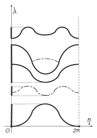
Figure 5: Graphs of eigenvalues of the problems in $\varpi^{0}$ and $\Pi$ with continuous and dotted lines, respectively. The spectral bands are the boldface vertical segments on the $\lambda$-axis.

$$\mathcal{B}_{k}^{\sharp}=\left\{\lambda=\lambda_{k}\left(\zeta\right):\zeta\in\left[\zeta_{k}^{-},\zeta_{k}^{+}\right]\subset\left[0,2\pi\right]\right\}\subset\mathbb{R}_{+}.$$ (3.37)

The segment (3.37) may be covered by a spectral band (2.15)=(3.33), or may intersect a spectral gap and in this case be contained in the additional part (1.25) of the essential spectrum $\sigma_{es}\left(\mathcal{A}\right)$ of the problem (1.18), (1.19); this fact has been mentioned in Section 1.4 and will be of interest later.

3.4 The regularity field for the open waveguide

We aim to verify the formula

$$\sigma_{es}\left(\mathcal{A}\right)=\sigma_{es}\left(\mathcal{A}^{0}\right)\cup\sigma^{\sharp},$$ (3.38)

and to this end we take a point $\lambda\in\overline{\mathbb{R}_{+}}$, which does not belong to set (3.38). Here, (3.38) contains the essential spectrum (2.16) of the purely periodic problem (1.4), (1.5) and also the union (cf. formula (1.26))

$$\sigma^{\sharp}={\displaystyle\bigcup_{\zeta\in\left[0,2\pi\right)}}\sigma_{di}\left(\mathcal{A}^{\sharp}\left(\zeta\right)\right)$$ (3.39)

of the discrete spectra of the operator family $\left\{\mathcal{A}^{\sharp}\left(\zeta\right)\right\}_{\zeta\in\left[0,2\pi\right)},$ (3.31). As explained above, the set (3.39) consists of a union of at most countably many segments (3.37).

Let the inhomogeneous problem (1.18), (1.19), namely

$$L\left(x,\nabla\right)u\left(x\right)-\lambda u\left(x\right) =f\left(x\right),\ \ \ x\in\Omega,$$ (3.40)

$$N\left(x,\nabla\right)u\left(x\right) =g\left(x\right),\ \ \ x\in\partial\Omega,$$

have the right-hand sides

$$\left\{f,g\right\}\in L^{2}\left(\Omega\right)^{n}\times H^{1/2}\left(\partial\Omega\right)^{n}.$$ (3.41)

We introduce a cut-off function $\mathcal{X}_{0}\in C^{\infty}\left(\mathbb{R}^{2}\right)$ such that

$$\mathcal{X}_{0}\left(x\right) =1\text{ for either }\left|x_{2}\right|>h+d\text{, or }x_{1}<-1-d,$$ (3.42)

$$\mathcal{X}_{0}\left(x\right) =0\text{ for }\left|x_{2}\right|<h\text{ and }x_{1}>-1,\ \ 0\leq\mathcal{X}_{0}\leq 1.$$

The function $\mathcal{X}_{0}$ is equal to 1 outside the semi-strip $\left(-1-d,+\infty\right)\times\left(-h-d,h+d\right)$ but vanishes inside the smaller semi-strip $\left(-1,+\infty\right)\times\left(-h,h\right)$ which contains $\varpi^{+}$ and thus also the open waveguide. Putting

$$f^{0}=\mathcal{X}_{0}f,\ \ \ \ g^{0}=\mathcal{X}_{0}g$$ (3.43)

gives us vector functions defined in $\Omega^{0}$ and $\partial\Omega^{0}$, respectively. Moreover,

$$\left\|f^{0};L^{2}\left(\Omega^{0}\right)\right\|\leq\left\|f;L^{2}\left(\Omega\right)\right\|,\ \ \ \left\|g^{0};H^{1/2}\left(\partial\Omega^{0}\right)\right\|\leq\left\|g;H^{1/2}\left(\partial\Omega\right)\right\|.$$ (3.44)

The first inequality (3.44) is evident, while the second one is a consequence of the following observation: in view of (3.42) and (1.3) the function $\mathcal{X}_{0}$ equals either one or zero on each connected component of the boundary $\partial\Omega^{0}.$ This also shows that the commutator $\left[N,\mathcal{X}_{0}\right]$ will be null the in second formula of (3.49).

Since $\lambda$ stays out of the set (3.38) by assumption, the condition (2.19) is met and, according to Section 2.3, the problem (2.19) gets a unique solution $u^{0}\in H^{2}\left(\Omega^{0}\right)^{n}$ with the estimate

$$\left\|u^{0};H^{2}\left(\Omega^{0}\right)\right\| \leq c\left(\left\|f^{0};L^{2}\left(\Omega^{0}\right)\right\|+\left\|g^{0};H^{1/2}\left(\partial\Omega^{0}\right)\right\|\right)\leq$$ (3.45)

$$\leq c\left(\left\|f;L^{2}\left(\Omega\right)\right\|+\left\|g;H^{1/2}\left(\partial\Omega\right)\right\|\right).$$

This solution forms the first component in the representation (notation will be introduced later step by step)

$$u=\mathcal{R}\left(\lambda\right)\left\{f,g\right\}=\mathcal{X}_{0}u^{0}+\mathcal{X}_{\sharp}u^{\sharp}+\mathcal{X}_{b}u^{b}$$ (3.46)

of a parametrix for the boundary-value problem (3.40); a parametrix is by definition a continuous operator

$$\mathcal{R}\left(\lambda\right):L^{2}\left(\Omega\right)^{n}\times H^{1/2}\left(\partial\Omega\right)^{n}\rightarrow H^{2}\left(\Omega\right)^{n}$$ (3.47)

such that the mapping

$$\left\{L,N\right\}\mathcal{R}\left(\lambda\right)-\mathbb{I}:L^{2}\left(\Omega\right)^{n}\times H^{1/2}\left(\partial\Omega\right)^{n}\rightarrow L^{2}\left(\Omega\right)^{n}\times H^{1/2}\left(\partial\Omega\right)^{n}$$ (3.48)

is compact, where $\mathbb{I}$ stands for the identity.

We have

$$L\left(\mathcal{X}_{0}u^{0}\right) =\mathcal{X}_{0}f^{0}+\left[L,\mathcal{X}_{0}\right]u^{0}=\mathcal{X}_{0}^{2}f+\left[L^{0},\mathcal{X}_{0}\right]u^{0},$$ (3.49)

$$N\left(\mathcal{X}_{0}u^{0}\right) =\mathcal{X}_{0}g^{0}=\mathcal{X}_{0}^{2}g,$$

where the term with the commutator $\left[L^{0},\mathcal{X}_{0}\right]$ admits the estimate

$$\left\|\left[L,\mathcal{X}_{0}\right]u^{0};H^{1}\left(\Omega\right)\right\| =\left\|\left[L^{0},\mathcal{X}_{0}\right]u^{0};H^{1}\left(\Omega^{0}\right)\right\|\leq$$ (3.50)

$$\leq c\left(\left\|f;L^{2}\left(\Omega\right)\right\|+\left\|g;H^{1/2}\left(\partial\Omega\right)\right\|\right).$$

The difference $u^{1}=u-u^{0}$ is to be sought from the problem

$$L\left(x,\nabla\right)u^{1}\left(x\right) =f^{1}\left(x\right)=\left(1-\mathcal{X}_{0}\left(x\right)^{2}\right)f\left(x\right)-\left[L,\mathcal{X}_{0}\right]u^{0}\left(x\right),\ \ \ x\in\Omega,$$ (3.51)

$$N\left(x,\nabla\right)u^{1}\left(x\right) =g^{1}\left(x\right)=\left(1-\mathcal{X}_{0}\left(x\right)^{2}\right)g\left(x\right),\ \ \ x\in\partial\Omega,$$

where the supports of the right-hand sides are located in the closed semi-infinite strip

$$\left[-1-d,+\infty\right)\times\left[-h-d,h+d\right].$$ (3.52)

We now introduce the cut-off function

$$\mathcal{X}_{\sharp}\left(x\right)=\chi\left(x_{1}-R\right),$$ (3.53)

where $\chi$ and $R$ are taken from (2.30) and (1.13), respectively. The products

$$f^{\sharp}=\mathcal{X}_{\sharp}f^{1},\ \ g^{\sharp}=\mathcal{X}_{\sharp}g^{1}$$ (3.54)

are defined in the domain $\Omega^{\sharp},$ see (3.3), and its boundary $\partial\Omega^{\sharp}.$ Moreover, the estimate

$$\left\|f^{\sharp};L_{\beta}^{2}\left(\Omega^{\sharp}\right)\right\|+\left\|g^{\sharp};W_{\beta}^{1/2}\left(\partial\Omega^{\sharp}\right)\right\| \leq c\left(\left\|f^{1};L^{2}\left(\Omega\right)\right\|+\left\|g^{1};H^{1/2}\left(\partial\Omega\right)\right\|\right)$$ (3.55)

$$\leq c\left(\left\|f;L^{2}\left(\Omega\right)\right\|+\left\|g;H^{1/2}\left(\partial\Omega\right)\right\|\right)$$

is valid with any weight index $\beta\in\mathbb{R}$, because $e^{\beta\left|x_{2}\right|}\leq c_{\beta}$ in the strip (3.52), where the supports of $f^{1}$ and $g^{1}$ are contained in.

We now make use of our assumption that $\lambda$ does not belong to the set (3.38). As a consequence, the operator $T_{\beta}\left(\lambda;\zeta\right)$ of the problem (3.11), (3.9) is an isomorphism between the weighted spaces in (3.17) for all

$$\zeta\in\left[0,2\pi\right)\text{ \ and \ }\beta\in\left[0,\beta_{0}\left(\lambda\right)\right),$$ (3.56)

where $\beta_{0}\left(\lambda\right)>0$ is determined in (3.23). In this way we apply the partial FBG-transform to the boundary-value problem (3.4) with the right-hand sides (3.54); this yields a problem of the form (3.11), (3.9), and we find a unique solution $U^{\sharp}\in W_{\beta,per\sharp}^{2}\left(\Pi\right)^{n}$ for it. The above mentioned isomorphism property of $T_{\beta}\left(\lambda;\zeta\right)$ guarantees the estimate

$$\int_{0}^{2\pi}\left\|U^{\sharp};W_{\beta,per\sharp}^{2}\left(\Pi\right)\right\|^{2}d\zeta \leq C\int_{0}^{2\pi}\left(\left\|F^{\sharp};L_{\beta}^{2}\left(\Pi\right)\right\|^{2}+\left\|G^{\sharp};W_{\beta}^{1/2}\left(\Gamma\right)\right\|^{2}\right)d\zeta$$ (3.57)

$$\leq c\left(\left\|f^{\sharp};L_{\beta}^{2}\left(\Omega^{\sharp}\right)\right\|^{2}+\left\|g^{\sharp};W_{\beta}^{1/2}\left(\partial\Omega^{\sharp}\right)\right\|^{2}\right),$$

where the latter inequality is based on (3.16) (and (3.4)). We then employ the inverse transform (3.10) and obtain a solution $u^{\sharp}\in W_{\beta}^{2}\left(\Omega^{\sharp}\right)^{n}$ together with the relation

$$\left\|u^{\sharp};H^{2}\left(\Omega^{\sharp}\right)\right\|^{2}\leq c_{\beta}\left\|u^{\sharp};W_{\beta}^{2}\left(\Omega^{\sharp}\right)\right\|^{2}\leq C_{\beta}\int_{0}^{2\pi}\left\|U^{\sharp};W_{\beta,per\sharp}^{2}\left(\Pi\right)\right\|^{2}d\zeta.$$ (3.58)

As a result, we have defined the second component in representation (3.46).

Remark 5

The same cut-off function (3.53) multiplies $u^{\sharp}$ in (3.46) as well as $f^{1}$ and $g^{1}$ in (3.54). In Section 4.4 we explain how the second term in (3.46) must be corrected in the case of the $\mathsf{L,V}$- and $\mathsf{Y,Z}$-shaped waveguides (see Fig. 3 and Section 1.5).

The estimates (3.58), (3.59) and (3.55) show that the product $\mathcal{X}_{\sharp}u^{\sharp}$ in (3.46) cannot prevent the continuity of the parametrix (3.47). Furthermore, we have

$$L\left(\mathcal{X}_{\sharp}u^{\sharp}\right) =\mathcal{X}_{\sharp}f^{\sharp}+\left[L,\mathcal{X}_{\sharp}\right]u^{\sharp}=\mathcal{X}_{\sharp}^{2}f^{1}+\left[L^{\sharp},\mathcal{X}_{\sharp}\right]u^{\sharp},$$ (3.59)

$$N\left(\mathcal{X}_{\sharp}u^{\sharp}\right) =\mathcal{X}_{\sharp}g^{\sharp}=\mathcal{X}_{\sharp}^{2}g^{1}$$

where

$$\left\|\left[L,\mathcal{X}_{\sharp}\right]u^{\sharp};W_{\beta}^{1}\left(\Omega^{\sharp}\right)\right\|\leq c\left\|u^{\sharp};W_{\beta}^{2}\left(\Omega^{\sharp}\right)\right\|\leq c\left(\left\|f;L^{2}\left(\Omega\right)\right\|+\left\|g;H^{1/2}\left(\partial\Omega\right)\right\|\right).$$ (3.60)

Since the supports of the coefficients in the operator $\left[L^{\sharp},\mathcal{X}_{\sharp}\right]$ are located in the vertical strip $\left\{x:x_{1}\in\left[R,R+d\right],\ x_{2}\in\mathbb{R}\right\},$ the exponential weight in the norm on the left-hand side of (3.60) helps to prove that the mapping

$$L^{2}\left(\Omega\right)^{n}\times H^{1/2}\left(\partial\Omega\right)^{n}\ni\left\{f,g\right\}\mapsto\left[L^{\sharp},\mathcal{X}_{\sharp}\right]u^{\sharp}\in L^{2}\left(\Omega\right)^{n}$$ (3.61)

is compact. Indeed, the mapping can be presented as a sum of a compact operator (due to the compact embedding $H^{1}\subset L^{2}$ in a bounded domain, the rectangle $\left[R,R+d\right]\times\left[-t,t\right]$), and a small operator with norm $O\left(e^{-t\beta}\right)$ (due to the weight which grows exponentially as $\left|x_{2}\right|>t$ and $t\rightarrow+\infty).$

All terms with the compact embedding property, e.g. (3.61), can be excluded from forthcoming considerations. Hence, owing to the inequality (3.50) and formulas (3.58), (3.59), it remains to deal with the problem (3.40) with compactly supported right-hand sides

$$f^{b}=\left(1-\mathcal{X}_{0}^{2}\right)\left(1-\mathcal{X}_{\sharp}^{2}\right)f,\ \ \ g^{b}=\left(1-\mathcal{X}_{0}^{2}\right)\left(1-\mathcal{X}_{\sharp}^{2}\right)g.$$

Since this problem is elliptic, recall Section 1.2, classical results in [1, 2] give a vector function $u^{b}\in H^{2}\left(\Omega\right)^{n}$ such that

$$L\left(\mathcal{X}_{b}u^{b}\right) =\mathcal{X}_{b}f^{b}+\left[L,\mathcal{X}_{b}\right]u^{b}=f^{b}+\left[L,\mathcal{X}_{b}\right]u^{b},$$

$$N\left(\mathcal{X}_{b}u^{b}\right) =\mathcal{X}_{b}g^{b}=g^{b},$$

$$\left\|u^{b};H^{2}\left(\Omega\right)\right\|+\left\|\left[L,\mathcal{X}_{b}\right]u^{b};H^{1}\left(\Omega\right)\right\| \leq c\left(\left\|f^{b};L^{2}\left(\Omega\right)\right\|+\left\|g^{b};H^{1/2}\left(\partial\Omega\right)\right\|\right)\leq$$

$$\leq c\left(\left\|f;L^{2}\left(\Omega\right)\right\|+\left\|g;H^{1/2}\left(\partial\Omega\right)\right\|\right),$$

where the cut-off function $\mathcal{X}_{b}$ can be chosen as

$$\mathcal{X}_{b}\left(x\right)={\displaystyle\prod_{\pm}}{\displaystyle\prod_{p=1,2}}\left(1-\chi\left(\pm x_{1}\mp\rho\right)\right)$$

and $\rho\in\mathbb{N}$ is sufficiently large.

So we have constructed the parametrix $\mathcal{R}\left(\lambda\right)$ with all necessary properties, see (3.47) and (3.48). Since the problem (3.40) is formally self-adjoint, we also have proved the following assertion which, in particular, shows that the given point $\lambda$ belongs to the regularity field of the operator $\mathcal{A}$ of Section 1.3.

Theorem 6

Assume $\lambda\in\overline{\mathbb{R}_{+}}\setminus\sigma_{es}\left(\mathcal{A}\right)$, cf. (3.38). The homogeneous problem (1.4), (1.5) has a finite-dimensional space $\ker\left(\mathcal{A}-\lambda\right)$ of solutions in $H^{2}\left(\Omega\right)^{n}.$ The inhomogeneous problem (3.40) admits a solution $u\in H^{2}\left(\Omega\right)^{n}$, if and only if the right-hand side (3.41) satisfies the compatibility conditions

$$\left(f,v\right)_{\Omega}+\left(g,v\right)_{\partial\Omega}=0,\ \ \ \forall v\in\ker\left(\mathcal{A}-\lambda\right).$$

This solution is defined up to an addendum in $\ker\left(\mathcal{A}-\lambda\right)$, and if in addition the orthogonality conditions

$$\left(u,v\right)_{\Omega}=0,\ \ \ \forall v\in\ker\left(\mathcal{A}-\lambda\right)$$

hold true, then it becomes unique and meets the estimate

$$\left\|u;H^{2}\left(\Omega\right)\right\|\leq c\left(\left\|f;L^{2}\left(\Omega\right)\right\|+\left\|g;H^{1/2}\left(\partial\Omega\right)\right\|\right).$$

3.5 The essential spectrum of the open waveguide

We now conclude with the main result of the paper.

Theorem 7

The essential spectrum of the operator $\mathcal{A}$ of the problem (1.18), (1.19) equals $\sigma_{es}\left(\mathcal{A}\right)=\sigma_{es}\left(\mathcal{A}^{0}\right)\cup\sigma^{\sharp}$, see (3.38), where the components $\sigma_{es}\left(\mathcal{A}^{0}\right)$ and $\sigma^{\sharp}$ are defined in Sections 2.2 and 3.3 by the formulas (2.16), (3.39), respectively.

Proof. Thanks to Theorem 6, it suffices to construct singular Weyl sequences for the operator $\mathcal{A}$ at all points in the set (3.38). If $\lambda\in\sigma_{es}\left(\mathcal{A}^{0}\right),$ we may take such a sequence from Section 2.4, because the support $\left[2^{j},2^{j+1}\right]\times\left[2^{j},2^{j+1}\right]$ of the cut-off function (2.31) and the entries (2.32) of the sequence do not touch the semi-strip $\left\{x:x_{1}>0,\ \left|x_{2}\right|<h\right\}$, where the open waveguide lies in.

Let $\lambda$ belong to the interior of segment (3.37), and recall that the endpoints live in $\sigma_{es}\left(\mathcal{A}^{0}\right)$, if they exist. By definition, there exists a $\zeta\in\left[0,2\pi\right)$ such that the problem (3.11), (3.9) admits a non-trivial solution $U^{\sharp}\in H_{\mathrm{per}\sharp}^{2}\left(\Pi\right)^{n}$; this generates a Floquet wave in the $x_{1}$-direction

$$u^{\sharp}\left(x\right)=e^{i\zeta x_{1}}U^{\sharp}\left(x\right)$$ (3.62)

satisfying the homogeneous ($f^{\sharp}=0,\ g^{\sharp}=0$) problem (3.4) in the periodic domain (3.3). By the constructions in Sections 1.3 and 3.1, this domain coincides with $\Omega$ in the half-plane $\left\{x:x_{1}>0\right\}$, where the matrices $A$ and $A^{\sharp}$ become equal to each other, see (1.16), (2.33), (3.1) and (1.15), (3.2). We localize the wave (3.62) by a cut-off function similar to (2.31), namely

$$X_{j}^{\sharp}\left(x\right)=\chi_{j}\left(x_{1}\right)\chi\left(x_{2}+2^{j+1}\right)\chi\left(2^{j+1}-x_{2}\right)$$ (3.63)

where $\chi_{j}$ and $\chi$ are taken from (2.29) and (2.30). The function $X_{j}^{\sharp}$ vanishes outside the rectangle $\left[2^{j},2^{j+1}\right]\times\left[-2^{j+1},2^{j+1}\right]$ and we will deal with indices $j\in\mathbb{N}$ such that $2^{j}>R,$ cf. (1.13). We set

$$v^{\sharp j}\left(x\right)=X_{j}^{\sharp}\left(x\right)u^{\sharp}\left(x\right),\ \ \ u^{\sharp j}\left(x\right)=\left\|v^{\sharp j};L^{2}\left(\Omega\right)\right\|^{-1}v^{\sharp j}\left(x\right)$$ (3.64)

and observe that, according to our choice of cut-off functions, both vector functions in (3.64) satisfy the boundary conditions (1.5).

Recall that by Theorem 3 the function $u^{\sharp}\left(x\right)$ decays exponentially as $x_{2}\rightarrow\pm\infty$, so we can compute the $L^{2}\left(\Omega\right)$-norm of $v^{\sharp j}$ as follows, cf. (2.33),

$$\left\|v^{\sharp j};L^{2}\left(\Omega\right)\right\|^{2} \geq\sum_{j=2^{j}+1}^{2^{j+1}-1}\int_{0}^{1}\int_{-2^{j+1}+1}^{2^{j+1}-1}\left|U^{\sharp}\left(x\right)\right|^{2}dx_{1}dx_{2}\geq$$ (3.65)

$$\geq\left(2^{j+1}-2^{j}-2\right)\left(\left\|U^{\sharp};L^{2}\left(\Pi\right)\right\|^{2}-C\exp\left(-2\beta 2^{j+1}\right)\right)\geq c_{\sharp}2^{j},\ \ c_{\sharp}>0.$$

We also obtain

$$f^{\sharp j}=Lv^{\sharp j}-\lambda v^{\sharp j}=L^{\sharp}v^{\sharp j}-\lambda v^{\sharp j}=\left[L^{\sharp},X_{j}^{\sharp}\right]u^{\sharp}$$ (3.66)

and notice that the supports of the coefficients in the commutator $\left[L^{\sharp},X_{j}^{\sharp}\right]$ belong to the union of two horizontal and two vertical rectangles of sizes $d\times 2^{j}$ and $2^{j+2}\times d$ respectively (they are overshadowed in Fig. 4, a). Due to the exponential decay of $u^{\sharp},$ the horizontal rectangles only cause an infinitesimal input into the $L^{2}\left(\Omega\right)$-norm of (3.66) as $j\rightarrow+\infty,$ and the input of the vertical ones stays uniformly bounded in $j.$ These mean that

$$\left\|\mathcal{A}u^{\sharp j}-\lambda u^{\sharp j};L^{2}\left(\Omega\right)\right\|=\left\|v^{\sharp j};L^{2}\left(\Omega\right)\right\|^{-1}\left\|f^{\sharp j};L^{2}\left(\Omega\right)\right\|\leq c2^{-j/2}.$$

An application of the Weyl criterion finishes the proof. $\blacksquare$

Remark 8

As was commented in Section 1.4, the set (3.39) in the representation (3.38) of $\sigma_{es}\left(\mathcal{A}\right)$ can have a non-empty intersection with the essential spectrum $\sigma_{es}\left(\mathcal{A}^{0}\right)$ of the problem (1.4), (1.5) in the purely periodic perforated plane $\Omega^{0}.$

4 Possible generalizations of the results

4.1 Concrete problems in mathematical physics

$(i)$ Scalar equations. Let $D\left(\nabla\right)=\nabla$ and let $A$ be a Hermitian, positive definite $2\times 2$-matrix function possessing the properties described in Section 1.3. Then $n=m=2$ and

$$L\left(x,\nabla_{x}\right)=-\nabla^{\top}A\left(x\right)\nabla$$ (4.1)

becomes an elliptic second-order differential operator in the divergence form. The algebraic completeness is evident, and in (1.9) we have $\varrho_{\nabla}=1$. We consider the following boundary conditions and problems: the Neumann condition

$$\nu\left(x\right)^{\top}A\left(x\right)\nabla u\left(x\right)=0,\ \ \ x\in\partial\Omega,$$ (4.2)

which is nothing but (1.5) with the co-normal derivative (1.8), and the Dirichlet boundary condition

$$u\left(x\right)=0,\ \ \ x\in\partial\Omega,$$ (4.3)

for the generalized Helmholtz equation

$$-\nabla^{\top}A\left(x\right)\nabla u\left(x\right)=\lambda\rho\left(x\right)u\left(x\right),\ \ \ x\in\Omega,$$ (4.4)

and the Steklov spectral problem

$$-\Delta u\left(x\right) =0,\ \ \ x\in\Omega,$$ (4.5)

$$\partial_{\nu}u\left(x\right) =\lambda u\left(x\right),\ \ \ x\in\partial\Omega,$$

where the spectral parameter $\lambda$ appears in the boundary condition while $\partial_{\nu}=\nu\left(x\right)^{\top}\nabla$ and $\Delta=\nabla^{\top}\nabla$ denote the outward normal derivative and the Laplace operator. The problem (4.4), (4.2) occurs in acoustics, and the problem (4.4), (4.3) with $L=\Delta$ and $A\left(x\right)=\mathbb{I}$ in the theory of quantum waveguides, see Remark 9 and [7, 8, 10, 12, 14]. Moreover, (4.5) is related to the linear theory of water waves, cf. [9, 30] and Remark 10.

$(ii)$ Elasticity. Let $n=2,$ $m=3$ and

$$D\left(\nabla\right)=\left(\begin{array}[c]{ccc}\partial_{1}&0&2^{-1/2}\partial_{2}\\ 0&\partial_{2}&2^{-1/2}\partial_{1}\end{array}\right)^{\top},\ \ \ \partial_{j}=\frac{\partial}{\partial x_{j}},\ \ j=1,2.$$ (4.6)

Interpreting $u=\left(u_{1},u_{2}\right)^{\top}$ as a displacement vector, we employ the Voigt-Mandel matrix notation in elasticity and introduce the strain and stress columns

$${\mbox{\boldmath$\varepsilon$}}\left(u;x\right) =\left({\mbox{\boldmath$\varepsilon$}}_{11}\left(u;x\right),{\mbox{\boldmath$\varepsilon$}}_{22}\left(u;x\right),2^{1/2}{\mbox{\boldmath$\varepsilon$}}_{12}\left(u;x\right)\right)^{\top}=D\left(\nabla\right)u\left(x\right),$$ (4.7)

$${\mbox{\boldmath$\sigma$}}\left(u;x\right) =A\left(x\right){\mbox{\boldmath$\varepsilon$}}\left(u;x\right)=A\left(x\right)D\left(\nabla\right)u\left(x\right),$$

which are composed from the Cartesian components ${\mbox{\boldmath$\varepsilon$}}_{jk}\left(u\right)=2^{-1}\left(\partial_{j}u_{k}+\partial_{k}u_{j}\right)$ and ${\mbox{\boldmath$\sigma$}}_{jk}\left(u\right)$ of the strain and stress tensors, respectively. Here, $A\left(x\right)$ stands for the Hooke matrix of elastic moduli, and it is real, symmetric, uniformly bounded and positive definite. The matrix $D\left(\nabla\right)$ in (4.6) is algebrically complete and $\varrho_{D}=2$ in (1.9), see [40, § 3.7.5] and, e.g., [35, Example 1.12], [11]. We assume that $A\left(x\right)$ meets all requirements listed in Section 1.3.

Time harmonic elastic waves with frequency $\kappa>0$ satisfy the system of differential equations

$$-\partial_{1}{\mbox{\boldmath$\sigma$}}_{j1}\left(u;x\right)-\partial_{2}{\mbox{\boldmath$\sigma$}}_{j2}\left(u;x\right)=\kappa^{2}\rho\left(x\right)u_{j}\left(x\right),\ \ \ j=1,2,\ \ x\in\Omega.$$ (4.8)

If $\rho\left(x\right)=const>0$ and $\lambda=\kappa^{2},$ system (4.8), in view of (4.7) and (4.6), takes form (1.4) while the traction-free boundary condition on $\partial\Omega$ reads as (1.5).

The problem on the oscillations of a homogeneous (constant $A$), perforated elastic plane is surely interesting for the engineering applications. To include composite elastic materials into our considerations, we must deal with the variable piecewise smooth Hooke matrix $A\left(x\right)$ and material density $\rho\left(x\right).$ Notice that the same modification can be applied to (4.4) as well. In the next section we will show how to get rid of the smoothness assumptions made until now when adapting our method to the variational formulation of the elasticity problem. Finally, as a possible application we also mention the Dirichlet problem (4.3) for the elastic displacement vector $u$, which has in the two-dimensional case a clear mechanical interpretation meaning that the boundaries of the holes in a thin elastic plate are rigidly clamped.

$(iii)$ Piezoelectricity. We set $n=3,$ $m=5$ and

$$D\left(\nabla\right)^{\top}=\left(\begin{array}[c]{cc}D^{\mathsf{M}}\left(\nabla\right)^{\top}&\mathbb{O}_{2\times 2}\\ \mathbb{O}_{1\times 3}&D^{\mathsf{E}}\left(\nabla\right)^{\top}\end{array}\right),\ \ \ \mathbb{E}=\left(\begin{array}[c]{ccc}1&0&0\\ 0&1&0\\ 0&0&0\end{array}\right)=diag\left\{1,1,0\right\},$$ (4.9)

where the $3\times 2$-block $D^{\mathsf{M}}\left(\nabla\right)$ is taken from (4.6) and $D^{\mathsf{E}}\left(\nabla\right)=\nabla.$ The column $u=\left(\begin{array}[c]{c}u^{\mathsf{M}}\\ u^{\mathsf{E}}\end{array}\right)$ consists of the displacement vector $u^{\mathsf{M}}=\left(u_{1},u_{2}\right)^{\top}$ and the electric potential $u^{\mathsf{E}}=u_{3}$ so that the superscripts $\mathsf{M}$ and $\mathsf{E}$ indicate mechanical and electric fields, respectively. The so-called smart piezo-devises are able to couple these fields of different physical nature, and this phenomenon is described by the following system of three differential equations, see [15, 41, 32],

$$D\left(-\nabla\right)^{\top}A\left(x\right)D\left(\nabla\right)u\left(x\right)=\lambda\rho\left(x\right)\mathbb{E}u\left(x\right),\ \ \ x\in\Omega.$$ (4.10)

Here, $\rho\left(x\right)>0$ is the material density and the matrix $A\left(x\right)$ is written blockwise as

$$A\left(x\right)=\left(\begin{array}[c]{cc}A^{\mathsf{MM}}\left(x\right)&A^{\mathsf{ME}}\left(x\right)\\ A^{\mathsf{EM}}\left(x\right)&-A^{\mathsf{EE}}\left(x\right)\end{array}\right),$$ (4.11)

where $A^{\mathsf{MM}}\left(x\right)$ denotes the elastic Hooke matrix, $A^{\mathsf{EE}}\left(x\right)$ the dielectric matrix and $A^{\mathsf{ME}}\left(x\right)=A^{\mathsf{EM}}\left(x\right)^{\top}$ the piezoelectric moduli. All matrices are real and $A^{\mathsf{MM}}\left(x\right)$ and $A^{\mathsf{EE}}\left(x\right)$ are symmetric positive definite, hence also the matrix (4.11) is symmetric, but it is not positive definite due to the minus sign in the bottom right-hand block. This reflects the intrinsic transformation of the elastic energy into the electric one and vice versa in a piezoelectric body. At the same time, the electric potential $u^{\mathsf{E}}$ does not affect the kinetic energy at low and middle frequencies and therefore it is absent on the right-hand side of (4.10), cf. structure of the diagonal matrix $\mathbb{E}$ in (4.9). We emphasize that in spite of the minus sign in (4.11) the piezoelectricity system (4.10) is elliptic in the Douglis-Nirenberg sense (cf. [35, Example 1.13]).

In Section 4.3 we demonstrate a reduction scheme from [36], which allows us to apply the above results to the piezoelectricity system with various boundary conditions.

$(iv)$ Plates. Let $n=3,$ $m=6$ and

$$D\left(\nabla\right)^{\top}=\left(\begin{array}[c]{cccccc}\partial_{1}&0&2^{-1/2}\partial_{2}&0&0&0\\ 0&\partial_{2}&2^{-1/2}\partial_{1}&0&0&0\\ 0&0&0&\partial_{1}^{2}&\partial_{1}^{2}&2^{1/2}\partial_{1}\partial_{2}\end{array}\right)=\left(\begin{array}[c]{cc}D^{\mathsf{M}}\left(\nabla\right)^{\top}&\mathbb{O}_{2\times 3}\\ \mathbb{O}_{1\times 3}&\nabla^{\top}D^{\mathsf{M}}\left(\nabla\right)^{\top}\end{array}\right).$$ (4.12)

The Dirichlet problem (4.10), (4.3) with matrices (4.12) and

$$A\left(x\right)=\left(\begin{array}[c]{cc}A^{\mathsf{MM}}\left(x\right)&A^{\mathsf{MB}}\left(x\right)\\ A^{\mathsf{BM}}\left(x\right)&A^{\mathsf{BB}}\left(x\right)\end{array}\right),\ \ \ \mathbb{E}=\left(\begin{array}[c]{ccc}0&0&0\\ 0&0&0\\ 0&0&1\end{array}\right)$$ (4.13)

describes the Kirchhoff model of an anisotropic inhomogeneous plate $\Omega$ with rigidly clamped boundaries of holes, which means

$$u\left(x\right)=0\in\mathbb{R}^{3},\ \ \ \partial_{\nu}u_{3}\left(x\right)=0,\ \ x\in\partial\Omega.$$ (4.14)

The vector $u=\left(u_{1},u_{2},u_{3}\right)^{\top}$ includes the longitudinal displacement $\left(u_{1},u_{2}\right)^{\top}$ and the deflection $u_{3}.$ The matrix $A\left(x\right)$ is real symmetric and positive definite, but in the case of elastic symmetry it becomes block-diagonal, i.e. $A^{\mathsf{MB}}=\left(A^{\mathsf{BM}}\right)^{\top}=\mathbb{O}_{3\times 3}.$ In this case the Douglis-Nirenberg system (4.10) decouples into two second-order equations and a fourth-order equation. In Section 4.3 we show that our scheme works also in the case of high-order differential equations including the Kirchhoff plate (see also [13]).

4.2 Operator formulation of the variational problem

The integral identity (1.20) corresponding to the spectral problem (1.18), (1.19) makes sense even in the case the matrix $A$ and scalar $\rho$ are just bounded, measurable, and the boundary $\partial\Omega$ is Lipschitz. It is important that all results on the solvability of model boundary value problems in Section 4.1 are easily adapted to their weak formulations in the Sobolev and Kondratiev spaces (see [31, Ch.2], and for the periodic case [37]). It is straightforward to include into our consideration any type of boundary conditions, which are covered by the symmetric Green formula (cf. [31, §2,2]), for example, the Dirichlet conditions (4.3) or mixed boundary conditions.

Remark 9

Lipschitz domains occur for example in the grating of quantum waveguides with long-haul thickening as in Fig. 6, a). Notice that the domain of the operator $\mathcal{A}$ differs from $H^{2}\left(\Omega\right)\cap H_{0}^{1}\left(\Omega\right),$ cf. [3] and, e.g., [39, Ch.2].

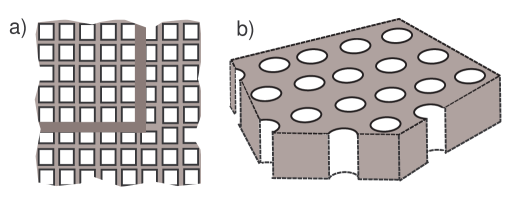
Figure 6: Other periodic geometries suitable for the present method.

If the density $\rho$ is not a constant, it is useful to change the operator formulation of the problem

$$\left(AD\left(\nabla\right)u,D\left(\nabla\right)v\right)_{\Omega}=\lambda\left(\rho u,v\right)_{\Omega},\ \ \ \forall v\in H^{1}\left(\Omega\right)^{n}$$ (4.15)

in order to apply the theory of self-adjoint operators in Hilbert space. Namely, having in mind the Korn inequality (1.17), we introduce in $\mathfrak{H}=H^{1}\left(\Omega\right)^{n}$ the specific scalar product

$$\left(u,v\right)_{\mathfrak{H}}=a\left(u,v;\Omega\right)+\left(\rho u,v\right)_{\Omega},$$ (4.16)

and then define the continuous, positive, symmetric, hence self-adjoint, operator $\mathcal{S}$ in $\mathfrak{H}$ by

$$\left(\mathcal{S}u,v\right)_{\mathfrak{H}}=\left(\rho u,v\right)_{\Omega},\ \ \ \forall u,v\in\mathfrak{H}.$$ (4.17)

This turns the problem (4.15) into the abstract equation

$$\mathcal{S}u=\varsigma u\text{ \ in }\mathfrak{H}$$ (4.18)

with the new spectral parameter

$$\varsigma=\left(1+\lambda\right)^{-1}.$$ (4.19)

The above-mentioned theory readily applies to the equation (4.18).

Remark 10

In the perforated plane $\Omega$ (where $\vartheta^{0}$ is not empty in (1.1) and (1.2)) also the Steklov problem (4.5) reduces to the equation (4.18) with parameter (4.19). According to [38] we endow in this case the space $H^{1}\left(\Omega\right)$ with the scalar product $\left(u,v\right)_{\mathfrak{H}}=\left(\nabla u,\nabla v\right)_{\Omega}+\left(u,v\right)_{\partial\Omega}$ and define the ”trace operator” $\mathcal{S}$ by $\left(\mathcal{S}u,v\right)_{\mathfrak{H}}=\left(u,v\right)_{\partial\Omega}.$

4.3 Reduction to integro-differential equations

Concerning the piezoelectricity problem with matrices (4.11), (4.9) or the plate problem with matrices (4.13), (4.12), we first mention that the results of the papers [33, 34] can be applied here, since they deal with general boundary value problems for Douglis-Nirenberg elliptic systems. However, the degenerate matrix $\mathbb{E}$ on the right-hand side of (4.10) hampers the use of the theory of self-adjoint operators in Hilbert space.

For the perforated Kirchhoff plate ($\vartheta^{0}\neq\emptyset$), the above mentioned trick works with the new scalar product and operator $\mathcal{S}$,

$$\left(u,v\right)_{\mathfrak{H}} =\left(AD\left(\nabla\right)u,D\left(\nabla\right)v\right)_{\Omega}+\left(\rho\mathbb{E}u,\mathbb{E}v\right)_{\Omega},$$ (4.20)

$$\left(\mathcal{S}u,v\right)_{\mathfrak{H}} =\left(\rho\mathbb{E}u,\mathbb{E}v\right)_{\Omega},\ \ \ \forall u,v\in\mathfrak{H}$$

where matrices are taken from (4.13) and (4.12). Indeed, owing to the Dirichlet clamping condition (4.14) the bilinear form (4.20) is a scalar product in $\mathfrak{H}=H_{0}^{1}\left(\Omega\right)^{2}\times H_{0}^{2}\left(\partial\Omega\right).$

The piezoelectricity problem (4.10), (1.5) requires a much more elaborate process. Following [36], we reduce the corresponding variational problem

$$\left(A^{\mathsf{MM}}D^{\mathsf{M}}\left(\nabla\right)u^{\mathsf{M}},D^{\mathsf{M}}\left(\nabla\right)v^{\mathsf{M}}\right)_{\Omega}+\left(A^{\mathsf{ME}}D^{\mathsf{E}}\left(\nabla\right)u^{\mathsf{E}},D^{\mathsf{M}}\left(\nabla\right)v^{\mathsf{M}}\right)_{\Omega}$$

$$\ \ +\left(A^{\mathsf{EM}}D^{\mathsf{M}}\left(\nabla\right)u^{\mathsf{M}},D^{\mathsf{E}}\left(\nabla\right)v^{\mathsf{E}}\right)_{\Omega}-\left(A^{\mathsf{EE}}D^{\mathsf{E}}\left(\nabla\right)u^{\mathsf{E}},D^{\mathsf{E}}\left(\nabla\right)v^{\mathsf{E}}\right)_{\Omega}$$

$$=\left(\rho u^{\mathsf{M}},v^{\mathsf{M}}\right)_{\Omega},\ \ \ \forall v\in H^{1}\left(\Omega\right)^{3}$$

to

$$\left(A^{\mathsf{MM}}D^{\mathsf{M}}\left(\nabla\right)u^{\mathsf{M}},D^{\mathsf{M}}\left(\nabla\right)v^{\mathsf{M}}\right)_{\Omega}+E\left(u^{\mathsf{M}},v^{\mathsf{M}}\right)=\left(\rho u^{\mathsf{M}},v^{\mathsf{M}}\right)_{\Omega},\ \ \ \forall v^{\mathsf{M}}\in H^{1}\left(\Omega\right)^{2},$$ (4.21)

where

$$E\left(u^{\mathsf{M}},v^{\mathsf{M}}\right)=\left(A^{\mathsf{ME}}D^{\mathsf{E}}\left(\nabla\right)Ru^{\mathsf{M}},D^{\mathsf{M}}\left(\nabla\right)v^{\mathsf{M}}\right)_{\Omega}$$ (4.22)

and $u^{\mathsf{E}}=Ru^{\mathsf{M}}\in\mathcal{H}^{1}\left(\Omega\right)$ is a solution of the scalar Neumann problem

$$\left(A^{\mathsf{EE}}D^{\mathsf{E}}\left(\nabla\right)u^{\mathsf{E}},D^{\mathsf{E}}\left(\nabla\right)v^{\mathsf{E}}\right)_{\Omega}$$

$$=\left(A^{\mathsf{EM}}D^{\mathsf{M}}\left(\nabla\right)u^{\mathsf{M}},D^{\mathsf{E}}\left(\nabla\right)v^{\mathsf{E}}\right)_{\Omega},\ \forall v^{\mathsf{E}}\in\mathcal{H}^{1}\left(\Omega\right).$$ (4.23)

Here, the space $\mathcal{H}^{1}\left(\Omega\right)$ is defined as a completion of $C_{c}^{\infty}\left(\overline{\Omega}\right)$ in the norm

$$\left(\left\|\nabla u^{\mathsf{E}};L^{2}\left(\Omega\right)\right\|^{2}+\left\|u^{\mathsf{E}};L^{2}\left(K\right)\right\|^{2}\right)^{1/2}$$

and $K$ is a compactum in $\overline{\Omega}$ of positive area. Since constants fall into $\mathcal{H}^{1}\left(\Omega\right),$ the problem (4.23) includes one compatibility condition, which is obviously met because the functional on the right-hand side of (4.23) degenerates on constants. In this way, the bilinear form (4.22) is well-defined, symmetric and positive, see [36] for details. Now the trick with a new scalar product in $\mathfrak{H}=H^{1}\left(\Omega\right)^{2}$ applies again.

Similar modifications work for other types of boundary conditions in piezoelectricity and plates as well.

4.4 Other geometries

To simplify the notation we have always used the covering of the plane with unit squares. The cells can as well be rectangles or parallelograms, because an affine transform does not change the crucial properties of the matrices $D\left(\nabla\right),$ $A\left(x\right)$ and operators (1.7), (1.8). We mention that according to [29], the elasticity problem in Section 4.1 $(ii)$ preserves its matrix form under any affine change of coordinates, though some special (non-physical!) columns of strains and stresses will then appear. A similar procedure applies to piezoelectricity and plates in Section 4.1 $(iii)$ and $(iv)$.

Other types of planar coverings can be treated in a similar manner, for instance, the diamond and honeycomb shapes, see [45]. We do not touch upon this generalization, which would require a total modification of the notation.

The purpose of the restriction (1.3) was solely to simplify the definitions of cut- off functions in (2.29)-(2.32) etc., but other settings of holes, cf. Fig. 7, a), can be treated by our method as well. We remark here that the homogeneous boundary conditions (1.5) and (1.19) are naturally included into the definitions of the domains (1.11) and (1.21) of the operators $\mathcal{A}^{0}$ and $\mathcal{A}$, and hence one has to take care that multiplication with the plateau functions (2.31) and (3.63) does not spoil these conditions, otherwise the arising discrepancies must be compensated. A simplest way to avoid the discrepancies is to construct cut-off functions, which respect the geometry and surround all holes, like indicated in Fig. 7, a), where the support of $\left|\nabla X_{j}\right|$ is shaded: no serious change of calculations would follow. Of course, no modification of cut-off functions is needed in the case of an intact periodic medium and Dirichlet conditions (4.3).

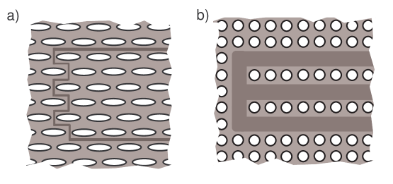
Figure 7: a) Perforation of another type. b) E-shaped open waveguide.

Our methods are sufficiently general to study the essential spectrum of the problem (1.18), (1.19) in the layer $\left\{x=\left(y,z\right):y=\left(y_{1},y_{2}\right)\in\mathbb{R}^{2},\ \left|z\right|<H\right\}$ perforated periodically and perturbed inside the semi-infinite cylinder $\mathbb{R}_{+}\times\left(-h,h\right)\times\left(-H,H\right),$ see Fig. 6, b). As in two-dimensional case, in this three-dimensional problem there again appear only two model spectral problems, one in a cell and another one in an infinite perforated prism, which can be examined with results in [45, 28] and [33, 39]. In particular our approach applies to elastic infinite three-dimensional plates, which are perforated or have periodic bases. On the other hand, our approach does not yet help to examine a problem in the space $\mathbb{R}^{3}$ with a triple-periodic perforation and with an open periodic waveguide inside a semi-infinity circular cylinder.

4.5 Joints of open waveguides

The waveguides depicted in Fig. 3 must keep the periodicity along all their branches so that axes of inclined branches in Fig. 3, a), c), cross the $x_{1}$-axis at angle $\phi$ with a rational $\tan\phi.$ Then each branch gives rise to its own model problem of type (3.11), (3.9) in a perforated strip $\Pi_{q}$ which is perpendicular to the branch axis and may have width different from the main period 1; here $q=1,...,Q$ and $Q$ is the number of branches. In this way the essential spectrum of problem (1.18), (1.19) for the joint of open waveguides becomes the union of $\sigma_{es}\left(\mathcal{A}^{0}\right)$ and the sets $\sigma_{1}^{\sharp},...,\sigma_{Q}^{\sharp}$ defined in (3.39) through the discrete spectra of the model problem in $\Pi_{1},...,\Pi_{Q}$ respectively. Theorem 7 remains true with this modification, but let us next comment the minor changes required for its proof.

First, let us reconsider the Weyl sequence in Section 2.4. Since there exists an unbounded angular opening between adjacent open waveguides, we can choose for any $j\in N$ a point $P^{j}=\left(P_{1}^{j},P_{2}^{j}\right)$ such that the support of the plateau function

$$X_{j}\left(x\right)=\chi_{j}\left(x_{1}-P_{1}^{j}\right)\chi_{j}\left(x_{2}-P_{2}^{j}\right)$$ (4.24)

intersects neither the open waveguides, nor supports of $X_{1},...,X_{j-1}.$ Using (4.24), the entries (2.32) of the Weyl singular will have all the properties listed in Section 2.4. Similarly, in Section 3.5 we shift the ”center” of the plateau function (3.63) along the branch axis and so obtain the Weyl sequence elements (3.64).

Second, the construction (3.46) of the parametrix (3.47) now involves the solutions $u_{\left(q\right)}^{\sharp}$ of (3.4) in the domains $\Omega_{j}^{\sharp}$ with the periodicity ”cell” $\Pi_{q};$ here $q=1,...,Q.$ These solutions should be located near their branches with the help of some cut-off functions $\mathcal{X}_{\sharp}^{q}$. However, the definition (3.53) does not work properly, since supp$\,\mathcal{X}_{\sharp}^{q}$ may intersect other branches of the joint and therefore new discrepancies may appear. To avoid these discrepancies one may place the plateau function between two neighboring branches as indicated in Fig. 4, b) by overshading. Since supp$\,\left|\nabla\mathcal{X}_{\sharp}^{q}\right|$ is located in a $\rho$-neighborhood of the sides of an angle domain, the exponential weight in the Kondratiev space still leads to compact mappings of type (3.61) and as a consequence the mapping (3.48) remains compact. Other steps in our proof of Theorem 7 remain unchanged.

We finally mention that in our notation the $\mathsf{E}$-shaped joint of open waveguide of Fig. 7, b), only has one branch, and therefore it is directly covered by Theorem 7.

Acknowledgements

G.Cardone is member of GNAMPA of INDAM. S.A. Nazarov was supported by the grant 0.38.237.2014 of St. Petersburg University and the Academy of Finland project ”Mathematical approach to band-gap engineering in piezoelectric and elasticity models”. J. Taskinen was supported by the Väisälä Foundation of the Finnish Academy of Sciences and Letters.

References

- [1] Agmon, S.; Douglis, A.; Nirenberg, L., Estimates near the boundary for solutions of elliptic partial differential equations satisfying general boundary conditions. I. Commun. Pure Appl. Math. 12, 623-727 (1959).
- [2] S. Agmon, A. Douglis, and L. Nirenberg, Estimates near the boundary for solutions of elliptic partial differential equations satisfying general boundary conditions, II. Comm. Pure Appl. Math. 17 (1964), pp. 35–92.
- [3] Birman, M.Sh.; Skvortsov, G.E., On square summability of highest derivatives of the solution of the Dirichlet problem in a domain with piecewise smooth boundary, Izv. Vyssh. Uchebn. Zaved., Mat. 1962, No.5 (30), 12-21.
- [4] Birman, M. Sh.; Solomjak, M. Z. Spectral theory of selfadjoint operators in Hilbert space. Translated from the 1980 Russian original by S. Khrushchëv and V. Peller. Mathematics and its Applications (Soviet Series). D. Reidel Publishing Co., Dordrecht, 1987.
- [5] Bonnet-Ben Dhia A.S., Dakhia G., Hazard C., Chorfi L., Diffraction by a defect in an open waveguide: a mathematical analysis based on a modal radiation condition, SIAM J. Appl. Math. 70, n. 3, 2009, 677–693.
- [6] Bonnet-Ben Dhia A.S., Goursaud B., Hazard C., Mathematical analysis of the junction of two acoustic open waveguides, SIAM J. Appl. Math. 71, n. 6, 2011, 2048-2071.
- [7] Borisov D., Cardone G., Planar waveguide with twisted boundary conditions: discrete spectrum, J. Math. Phys. 52, n. 12, 2011, 123513.
- [8] Borisov D., Cardone G., Complete asymptotic expansions for the eigenvalues of the Dirichlet Laplacian in thin three-dimensional rods, ESAIM Control Optim. Calc. Var. 17, 2011, 887 908.
- [9] Cardone G., Durante T., Nazarov S.A., Water-waves modes trapped in a canal by a body with the rough surface, ZAMM Z. Angew. Math. Mech. 90, n. 12, 2010, 983 1004.
- [10] Cardone G., Khrabustowskyi A., Neumann spectral problem in a domain with very corrugated boundary, J. Differ. Equ. 259, n. 6, 2015, 2333 2367.
- [11] Cardone G., Minutolo V., Nazarov S.A., Gaps in the essential spectrum of periodic elastic waveguides, ZAMM Z. Angew. Math. Mech. 89, n. 9, 2009, 729 741.
- [12] Cardone G., Nazarov S.A., Perugia C., A gap in the continuous spectrum of a cylindrical waveguide with a periodic perturbation of the surface, Math. Nachr. 283, n. 9, 2010, 1222 1244.
- [13] Cardone G., Nazarov S.A., Piatnitski A.L., On the rate of convergence for perforated plates with a small interior Dirichlet zone, Z. Angew. Math. Phys. 62, n. 3, 2011, 439 468.
- [14] Cardone G., Nazarov S.A., Ruotsalainen K., Bound states of a converging quantum waveguide, ESAIM Math. Model. Numer. Anal. 47, n. 1, 2013, 305 315.
- [15] Cardone G., Nazarov S.A., Sokolowski J., Asymptotic analysis, polarization matrices and topological derivatives for piezoelectric materials with small voids, SIAM J. Control Optim. 48, n. 6, 2010, 3925 3961.
- [16] Carini J. P., Londergan J. T., Murdock D. P., Binding and scattering in two-dimensional systems: applications to quantum wires, waveguides, and photonic crystals, Springer Lecture Notes in Physics series, Berlin: Springer-Verlag 1999.
- [17] Englisch, H., Kirsch, W., Schröder, M.; Simon, B., Random Hamiltonians ergodic in all but one direction. Comm. Math. Phys. 128 (1990), no. 3, 613–625.
- [18] Friedlander L., Absolute continuity of the spectra of periodic waveguides, Contemp. Math. 339, 2003, 37–42.
- [19] Gel’fand I.M. Expansions in eigenfunctions of an equation with periodic coefficients. Dokl. Acad. Nauk SSSR. 1950. V. 73. P. 1117–1120.
- [20] Gohberg, I. C.; Kreĭn, M. G. Introduction to the theory of linear nonselfadjoint operators in Hilbert space, Nauka, Moscow 1965 (Engl. Transl.: Translations of Mathematical Monographs, Vol. 18 American Mathematical Society, Providence, R.I. 1969).
- [21] Hempel, R., Kohlmann, M., Spectral properties of grain boundaries at small angles of rotation. J. Spectr. Theory 1 (2011), no. 2, 197–219.
- [22] Hempel, R., Kohlmann, M., Dislocation problems for periodic Schrödinger operators and mathematical aspects of small angle grain boundaries. Spectral theory, mathematical system theory, evolution equations, differential and difference equations, 421–432, Oper. Theory Adv. Appl., 221, Birkhäuser/Springer Basel AG, Basel, 2012.
- [23] Hille, E., Phillips, R.S: Functional analysis and semi-groups, American Mathematical Society Colloquium publications 31 (1957)
- [24] Kachkovskii I.V., Filonov N.D., Absolute continuity of the spectrum of a periodic Schrödinger operator in a multidimensional cylinder, Algebra i Analiz, 21 (1) (2009) 133–152, English transl.: St. Petersbg. Math. J. 21 (1) (2010) 95-109.
- [25] Kato T., Perturbation Theory for linear operator edition, Grundlehren der Mathematischen Wissenschaften, Band 132, Springer-New York, 1976, xxi+619 pp.
- [26] Kondratiev V.A., Boundary problems for elliptic equations in domains with conical or angular points, Trudy Moskov. Mat.Obshch. 16 (1967) 209-292. (Engl. transl. in Trans. Moscow Math. Soc. 16 (1967), 227-313).
- [27] Kuchment P.A., Floquet theory for partial differential equations. (Russian) Uspekhi Mat. Nauk 37 (1982), no. 4 (226), 3–52, 240.
- [28] Kuchment P.A., Floquet theory for partial differential equations. Operator Theory: Advances and Applications, 60. Birkhäuser Verlag, Basel, 1993.
- [29] Kulikov A.A., Nazarov S.A., Narbut M.A. Linear transformations for the plane problem of anisotropic theory of elasticity, Vestnik St.-Petersburg Univ. 2000. N 2. P. 91-95.
- [30] Kuznetsov N., Maz’ya V., Vainberg B., Linear Water Waves. Cambridge: Cambridge University Press. 2002.
- [31] Lions J.L., Magenes E., Non-homogeneous boundary value problems and applications, Springer-Verlag, New York-Heidelberg, 1972.
- [32] Maugin, G.A., Nonlinear electromechanical effects and applications, Series in Theoretical and Applied Mechanics, 1. World Scientific Publishing Co., Philadelphia, PA, 1985.
- [33] Nazarov S.A. Elliptic boundary value problems with periodic coefficients in a cylinder, Izv. Akad. Nauk SSSR. Ser. Mat. 1981. V. 45, N 1. P. 101-112. (English transl.: Math. USSR. Izvestija. 1982. V. 18, N 1. P. 89-98)
- [34] Nazarov S.A. A Dirichlet problem for an elliptic system with periodic coefficients in the angular domain, Vestnik Leningrad. Univ. 1990. N 1. P. 32-35. (English transl.: Vestn. Leningr. Univ. Math. 1990. V. 23, N 1. P. 33-35)
- [35] Nazarov S.A., The polynomial property of self-adjoint elliptic boundary-value problems and the algebraic description of their attributes, Uspehi mat. nauk., 54, (5) 1999, 77-142. (English transl.: Russ. Math. Surveys, 54, (5) 1999, 947-1014).
- [36] Nazarov S.A. Uniform estimates of remainders in asymptotic expansions of solutions to the problem on eigen-oscillations of a piezoelectric plate // Probl. mat. analiz. N 25. Novosibirsk: Nauchnaya kniga, 2003. P. 99-188. (English transl.: Journal of Math. Sci., 2003. V.114, N. 5. P. 1657-1725.)
- [37] Nazarov S.A. Properties of spectra of boundary value problems in cylindrical and quasicylindrical domains, Sobolev Spaces in Mathematics. V. II (Maz’ya V., Ed.) International Mathematical Series , Vol. 9. New York: Springer, 2008. P. 261–309.
- [38] Nazarov S.A., Sufficient conditions for the existence of trapped modes in problems of linear theory of surface waves, Zap. Nauchn. Sem. S.-Peterburg. Otdel. Mat. Inst. Steklov. (POMI) 369 (2009), Matematicheskie Voprosy Teorii Rasprostraneniya Vol. 38, 202–223, 227; J. Math. Sciences, 167, n. 5, 2010, 713-725.
- [39] Nazarov S.A., Plamenevsky B.A., Elliptic problems in domains with piecewise smooth boundaries. Moscow: Nauka. 1991; English transl.: Nazarov, Sergey A.; Plamenevsky, Boris A. Elliptic problems in domains with piecewise smooth boundaries. de Gruyter Expositions in Mathematics, 13. Walter de Gruyter & Co., Berlin, 1994.
- [40] Nečas J., Direct methods in the theory of elliptic equations. Springer, Heidelberg - Dordrecht- London - New York, 2012.
- [41] Parton, V.Z., Kudriavtsev, B.A., Electromagnetoelasticity: Piezoelectrics and Electrically Conductive Solids. Gordon & Breach Science Publishers, New York, 1988.
- [42] Reed M., Simon B., Methods of modern mathematical physics. I: Functional Analysis. Academic Press, New York - San Francisco - London, 1992.
- [43] Reed M., Simon B., Methods of modern mathematical physics. IV: Analysis of operators. Academic Press, New York - San Francisco - London,
- [44] Rudin, W., Functional analysis. McGraw-Hill Book Company, New York, 1973.
- [45] Skriganov M.M., Geometric and arithmetic methods in the spectral theory of multidimensional periodic operators, Trudy Mat. Inst. Steklov 171 (1985) (English transl.: Proc. Steklov Inst. Math. 171 (2), vi–121 (1987)).
- [46] Thomas L., Time dependent approach to scattering from impurities in a crystal, Commun. Math. Phys. 33, 1973, 335–343.