Deep Broad Learning - Big Models for Big Data

Abstract

Deep learning has demonstrated the power of detailed modeling of complex high-order (multivariate) interactions in data. For some learning tasks there is power in learning models that are not only Deep but also Broad. By Broad, we mean models that incorporate evidence from large numbers of features. This is of especial value in applications where many different features and combinations of features all carry small amounts of information about the class. The most accurate models will integrate all that information. In this paper, we propose an algorithm for Deep Broad Learning called DBL. The proposed algorithm has a tunable parameter $n$, that specifies the depth of the model. It provides straightforward paths towards out-of-core learning for large data. We demonstrate that DBL learns models from large quantities of data with accuracy that is highly competitive with the state-of-the-art.

Keywords: Classification, Big Data, Deep Learning, Broad Learning, Discriminative-Generative Learning, Logistic Regression, Extended Logistic Regression

1 Introduction

The rapid growth in data quantity (Ganz and Reinsel, 2012) makes it increasingly difficult for machine learning to extract maximum value from current data stores. Most state-of-the-art learning algorithms were developed in the context of small datasets. However, the amount of information present in big data is typically much greater than that present in small quantities of data. As a result, big data can support the creation of very detailed models that encode complex higher-order multivariate distributions, whereas, for small data, very detailed models will tend to overfit and should be avoided (Brain and Webb, 2002; Martinez et al., 2015). We highlight this phenomenon in Figure 1. We know that the error of most classifiers decreases as they are provided with more data. This can be observed in Figure 1 where the variation in error-rate of two classifiers is plotted with increasing quantities of training data on the poker-hand dataset (Frank and Asuncion, 2010). One is a low-bias high-variance learner (KDB $k=5$, taking into account quintic features, (Sahami, 1996)) and the other is a low-variance high-bias learner (naive Bayes, a linear classifier). For small quantities of data, the low-variance learner achieves the lowest error. However, as the data quantity increases, the low-bias learner comes to achieve the lower error as it can better model higher-order distributions from which the data might be sampled.

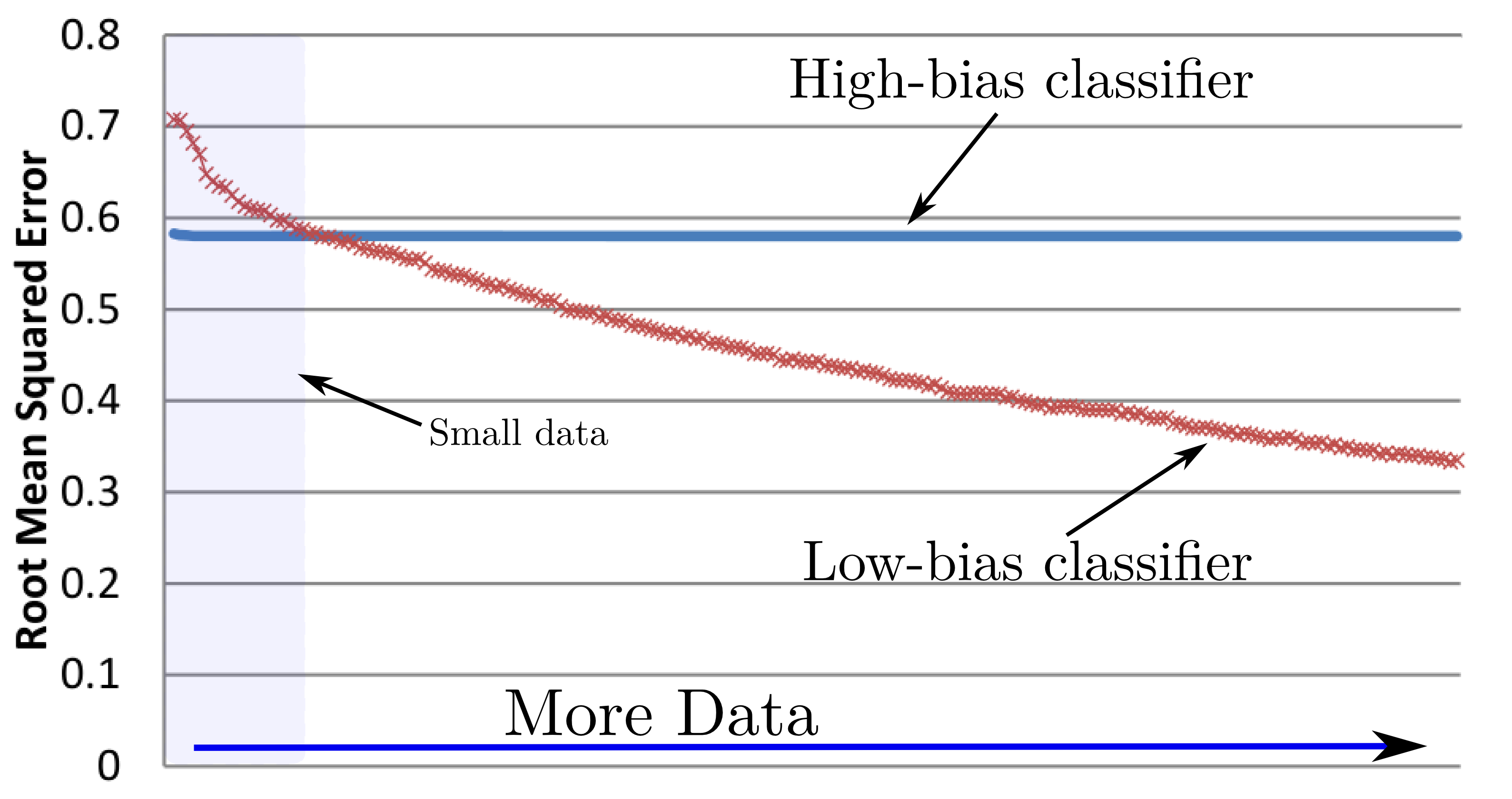
Figure 1: Comparative study of the error committed by high- and low-bias classifiers on increasing quantities of data.

The capacity to model different types of interactions among variables in the data is a major determinant of a learner’s bias. The greater the capacity of a learner to model differing distributions, the lower its bias will tend to be. However, many learners have limited capacity to model complex higher-order interactions.

Deep learning has demonstrated some remarkable successes through its capacity to create detailed (deep) models of complex multivariate interactions in structured data (e.g., data in computer vision, speech recognition, bioinformatics, etc.). Deep learning can be characterized in several different ways. But the underlying theme is that of learning higher-order interactions among features using a cascade of many layers. This process is known as ‘feature extraction’ and can be un-supervised as it leverages the structure within the data to create new features. Higher-order features are created from lower-order features creating a hierarchical structure. We conjecture that the deeper the model the higher the order of interactions that are captured in the data and the lower the bias that the model exhibits.

We argue that in many domains there is value in creating models that are broad as well as deep. For example, when using web browsing history, or social network likes, or when analyzing text, it is often the case that each feature provides only extremely small amounts of information about the target class. It is only by combining very large amounts of this micro-evidence that reliable classification is possible.

We call a model broad if it utilizes large numbers of variables. We call a model deep and broad if it captures many complex interactions each between numerous variables. For example, typical linear classifiers such as Logistic Regression (LR) and Naive Bayes (NB) are Broad Learners, in that they utilize all variables. However, these models are not deep, as they do not directly model interactions between variables. In contrast, Logistic Regression with cubic features ($\text{LR}^{3}$) (Langford et al., 2007) and Averaged 2-Dependence Estimators (A2DE) (Webb et al., 2011; Zaidi and Webb, 2012), both of which consider all combinations of 3 variables, are both Deep and Broad. The parameters of the former are fit discriminatively through computationally intensive gradient descent-based search, while the parameters of the latter are fit generatively using computationally efficient maximum-likelihood estimation. This efficient estimation of A2DE parameters makes it computationally well-suitable for big data. In contrast, we argue that $\text{LR}^{3}$’s discriminative parameterization can more closely fit the data than A2DE, making it lower bias and hence likely to have lower error when trained on large training sets. However, the computation required to optimize the parameters for $\text{LR}^{3}$ becomes computationally intensive even on moderate dimensional data.

Recently, it has been shown that it is possible to form a hybrid generative-discriminate learner that exploits the strengths of both naive Bayes (NB) and Logistic Regression (LR) by creating a weighted variant of NB in which the weights are optimized using discriminative minimization of conditional log-likelihood (Zaidi et al., 2013, 2014). From one perspective, the resulting learner can be viewed as using weights to alleviate the attribute independence assumption of NB. From another perspective it can be seen to use the maximum likelihood parameterization of NB to pre-condition the discriminative search of LR. The result is a learner that learns models that are exactly equivalent to LR, but does so much more efficiently.

In this work, we show how to achieve the same result with $\text{LR}^{n}$, creating a hybrid generative-discriminative learner named $\text{DBL}^{n}$ for categorical data that learns equivalent deep broad models to those of $\text{LR}^{n}$, but does so more efficiently. We further demonstrate that the resulting models have low bias and have very low error on large quantities of data. However, to create this hybrid learner we must first create an efficient generative counterpart to $\text{LR}^{n}$.

In short, the contributions of this work are:

• developing an efficient generative counter-part to $\text{LR}^{n}$, named Averaged $n$-Join Estimators (AnJE),

• developing $\text{DBL}^{n}$, a hybrid of $\text{LR}^{n}$ and AnJE,

• demonstrating that $\text{DBL}^{n}$ has equivalent error to LRⁿ, but is more efficient,

• demonstrating that $\text{DBL}^{n}$ has low error on large data.

2 Notation

We seek to assign a value $y\in\Omega_{Y}=\{y_{1},\ldots y_{C}\}$ of the class variable $Y$, to a given example $\mathbf{x}=(x_{1},\ldots,x_{a})$, where the $x_{i}$ are value assignments for the $a$ attributes $\mathcal{A}=\{X_{1},\ldots,X_{a}\}$. We define $\mathcal{A}\choose n$ as the set of all subsets of $\mathcal{A}$ of size $n$, where each subset in the set is denoted as $\alpha$:

$${\mathcal{A}\choose n}=\{\alpha\subseteq\mathcal{A}:|\alpha|=n\}.$$

We use $x_{\alpha}$ to denote the set of values taken by attributes in the subset $\alpha$ for any data object $\mathbf{x}$.

LR for categorical data learns a weight for every attribute value per class. Therefore, for LR, we denote, $\beta_{y}$ to be the weight associated with class $y$, and $\beta_{y,i,x_{i}}$ to be the weight associated with attribute $i$ taking value $x_{i}$ with class label $y$. For $\text{LR}^{n}$, $\beta_{y,\alpha,x_{\alpha}}$ specifies the weight associated with class $y$ and attribute subset $\alpha$ taking value $x_{\alpha}$. The equivalent weights for $\text{DBL}^{n}$ are denoted by $w_{y}$, $w_{y,i,x_{i}}$ and $w_{y,\alpha,x_{\alpha}}$.

The probability of attribute $i$ taking value $x_{i}$ given class $y$ is denoted by ${\rm P}(x_{i}\,|\,y)$. Similarly, probability of attribute subset $\alpha$, taking value $x_{\alpha}$ is denoted by ${\rm P}(x_{\alpha}|y)$.

3 Using generative models to precondition discriminative learning

There is a direct equivalence between a weighted NB and LR (Zaidi et al., 2013, 2014). We write LR for categorical features as:

$${\rm P}_{\!\textit{LR}}(y\mathchoice{\hskip 1.0pt}{\hskip 0.75pt}{\hskip 0.5pt}{\hskip 0.33pt}|\mathchoice{\hskip 1.0pt}{\hskip 0.75pt}{\hskip 0.5pt}{\hskip 0.33pt}{\bf x})=\exp\mathopen{}\Big{(}\beta_{y}+\sum_{i=1}^{a}\beta_{y,i,x_{i}}-\log\!\!\sum_{c\in\Omega_{Y}}\!\!\exp\mathopen{}\Big{(}\beta_{c}+\sum_{j=1}^{a}\beta_{c,j,x_{j}}\Big{)}\Big{)}$$ (1)

and NB as:

$${\rm P}_{\!\textit{NB}}(y\mathchoice{\hskip 1.0pt}{\hskip 0.75pt}{\hskip 0.5pt}{\hskip 0.33pt}|\mathchoice{\hskip 1.0pt}{\hskip 0.75pt}{\hskip 0.5pt}{\hskip 0.33pt}{\bf x})=\frac{{\rm P}(y)\prod_{i=1}^{a}{\rm P}(x_{i}\mathchoice{\hskip 1.0pt}{\hskip 0.75pt}{\hskip 0.5pt}{\hskip 0.33pt}|\mathchoice{\hskip 1.0pt}{\hskip 0.75pt}{\hskip 0.5pt}{\hskip 0.33pt}y)}{\sum_{c\in\Omega_{Y}}{\rm P}(c)\prod_{i=1}^{a}{\rm P}(x_{i}\mathchoice{\hskip 1.0pt}{\hskip 0.75pt}{\hskip 0.5pt}{\hskip 0.33pt}|\mathchoice{\hskip 1.0pt}{\hskip 0.75pt}{\hskip 0.5pt}{\hskip 0.33pt}c)}.$$

One can add the weights in NB to alleviate the attribute independence assumption, resulting in the WANBIA-C formulation, that can be written as:

$${\rm P}_{\!\textit{W}}(y\mathchoice{\hskip 1.0pt}{\hskip 0.75pt}{\hskip 0.5pt}{\hskip 0.33pt}|\mathchoice{\hskip 1.0pt}{\hskip 0.75pt}{\hskip 0.5pt}{\hskip 0.33pt}{\bf x}) =\frac{{\rm P}(y)^{w_{y}}\prod_{i=1}^{a}{\rm P}(x_{i}\mathchoice{\hskip 1.0pt}{\hskip 0.75pt}{\hskip 0.5pt}{\hskip 0.33pt}|\mathchoice{\hskip 1.0pt}{\hskip 0.75pt}{\hskip 0.5pt}{\hskip 0.33pt}y)^{w_{y,i,x_{i}}}}{\sum_{c\in\Omega_{Y}}{\rm P}(c)^{w_{c}}\prod_{j=1}^{a}{\rm P}(x_{i}\mathchoice{\hskip 1.0pt}{\hskip 0.75pt}{\hskip 0.5pt}{\hskip 0.33pt}|\mathchoice{\hskip 1.0pt}{\hskip 0.75pt}{\hskip 0.5pt}{\hskip 0.33pt}c)^{w_{c,j,x_{j}}}}$$

$$=\exp\mathopen{}\Big{(}w_{y}\log{\rm P}(y)+\sum_{i=1}^{a}w_{y,i,x_{i}}\log{\rm P}(x_{i}\mathchoice{\hskip 1.0pt}{\hskip 0.75pt}{\hskip 0.5pt}{\hskip 0.33pt}|\mathchoice{\hskip 1.0pt}{\hskip 0.75pt}{\hskip 0.5pt}{\hskip 0.33pt}y)-$$

$$\log\sum_{c\in\Omega_{Y}}\exp\mathopen{}\Big{(}w_{c}\log{\rm P}(c)+\sum_{j=1}^{a}\!w_{c,j,x_{j}}\log{\rm P}(x_{j}\!\mathchoice{\hskip 1.0pt}{\hskip 0.75pt}{\hskip 0.5pt}{\hskip 0.33pt}|\mathchoice{\hskip 1.0pt}{\hskip 0.75pt}{\hskip 0.5pt}{\hskip 0.33pt}c)\Big{)}\Big{)}.$$ (2)

When conditional log likelihood (CLL) is maximized for LR and weighted NB using Equation 1 and 2 respectively, we get an equivalence such that $\beta_{c}\propto w_{c}\log{\rm P}(c)$ and $\beta_{c,i,x_{i}}\propto w_{c,i,x_{i}}\log{\rm P}(x_{i}\mathchoice{\hskip 1.0pt}{\hskip 0.75pt}{\hskip 0.5pt}{\hskip 0.33pt}|\mathchoice{\hskip 1.0pt}{\hskip 0.75pt}{\hskip 0.5pt}{\hskip 0.33pt}c)$. Thus, WANBIA-C and LR generate equivalent models. While it might seem less efficient to use WANBIA-C which has twice the number of parameters of LR, the probability estimates are learned very efficiently using maximum likelihood estimation, and provide useful information about the classification task that in practice serve to effectively precondition the search for the parameterization of weights to maximize conditional log likelihood.

4 Deep Broad Learner (DBL)

In order to create an efficient and effective low-bias learner, we want to perform the same trick that is used by WANBIA-C for LR with higher-order categorical features. We define $\text{LR}^{n}$ as:

$${\rm P}_{\!\textit{LR}^{n}}\!(y\mathchoice{\hskip 1.0pt}{\hskip 0.75pt}{\hskip 0.5pt}{\hskip 0.33pt}|\mathchoice{\hskip 1.0pt}{\hskip 0.75pt}{\hskip 0.5pt}{\hskip 0.33pt}{\bf x})=\frac{\exp\mathopen{}\big{(}\beta_{y}+\sum_{\alpha\in{\mathcal{A}\choose n}}\beta_{y,\alpha,x_{\alpha}}\big{)}}{\sum_{c\in\Omega_{Y}}\exp\mathopen{}\big{(}\beta_{c}+\sum_{\alpha^{*}\in{\mathcal{A}\choose n}}\beta_{c,\alpha^{*},x_{\alpha^{*}}}\big{)}}.$$ (3)

We do not include lower-order terms. For example, if $n=2$ we do not include terms for $\beta_{y,i,x_{i}}$ as well as for $\beta_{y,i,x_{i},j,x_{j}}$, because doing so does not increase the space of distinct distributions that can be modeled but does increase the number of parameters that must be optimized.

To precondition this model using generative learning, we need a generative model of the form

$${\rm P}(y\hskip 1.5pt|\hskip 1.5pt{\bf x}) =\frac{{\rm P}(y)\prod_{\alpha\in{\mathcal{A}\choose n}}{\rm P}(x_{\alpha}\mathchoice{\hskip 1.0pt}{\hskip 0.75pt}{\hskip 0.5pt}{\hskip 0.33pt}|\mathchoice{\hskip 1.0pt}{\hskip 0.75pt}{\hskip 0.5pt}{\hskip 0.33pt}y)}{\prod_{c\in\Omega_{Y}}\mathopen{}\left({\rm P}(c)\prod_{\alpha^{*}\in{\mathcal{A}\choose n}}{\rm P}(x_{\alpha^{*}}\mathchoice{\hskip 1.0pt}{\hskip 0.75pt}{\hskip 0.5pt}{\hskip 0.33pt}|\mathchoice{\hskip 1.0pt}{\hskip 0.75pt}{\hskip 0.5pt}{\hskip 0.33pt}c)\right)\mathclose{}}$$ (4)

$$=\exp\mathopen{}\Big{(}\log{\rm P}(y)+\sum_{\alpha\in{\mathcal{A}\choose n}}\log{\rm P}(x_{\alpha}\mathchoice{\hskip 1.0pt}{\hskip 0.75pt}{\hskip 0.5pt}{\hskip 0.33pt}|\mathchoice{\hskip 1.0pt}{\hskip 0.75pt}{\hskip 0.5pt}{\hskip 0.33pt}y)-$$

$$\quad\log\!\sum_{c\in\Omega_{Y}}\exp\mathopen{}\Big{(}\log{\rm P}(c)+\sum_{\alpha^{*}\in{\mathcal{A}\choose n}}\log{\rm P}(x_{\alpha^{*}}\mathchoice{\hskip 1.0pt}{\hskip 0.75pt}{\hskip 0.5pt}{\hskip 0.33pt}|\mathchoice{\hskip 1.0pt}{\hskip 0.75pt}{\hskip 0.5pt}{\hskip 0.33pt}c)\Big{)}\Big{)}.$$ (5)

The only existing generative model of this form is a log-linear model, which requires computationally expensive conditional log-likelihood optimization and consequently would not be efficient to employ. It is not possible to create a Bayesian network of this form as it would require that ${\rm P}(x_{i},x_{j})$ be independent of ${\rm P}(x_{i},x_{k})$. However, we can use a variant of the AnDE (Webb et al., 2011, 2005) approach of averaging many Bayesian networks. Unlike AnDE, we cannot use the arithmetic mean, as we require a product of terms in Equation 4 rather than a sum, so we must instead use a geometric mean.

4.1 Averaged n-Join Estimators (AnJE)

Let $\mathcal{P}$ be a partition of the attributes $\mathcal{A}$. By assuming independence only between the sets of attributes $A\in\mathcal{P}$ one obtains an n-joint estimator:

$${\rm P}_{\textrm{AnJE}}({\bf x}\mathchoice{\hskip 1.0pt}{\hskip 0.75pt}{\hskip 0.5pt}{\hskip 0.33pt}|\mathchoice{\hskip 1.0pt}{\hskip 0.75pt}{\hskip 0.5pt}{\hskip 0.33pt}y)=\prod_{\alpha\in\mathcal{P}}{\rm P}(x_{\alpha}\mathchoice{\hskip 1.0pt}{\hskip 0.75pt}{\hskip 0.5pt}{\hskip 0.33pt}|\mathchoice{\hskip 1.0pt}{\hskip 0.75pt}{\hskip 0.5pt}{\hskip 0.33pt}y).$$

For example, if there are four attributes $X_{1}$, $X_{2}$ , $X_{3}$ and $X_{4}$ that are partitioned into the sets $\{X_{1},X_{2}\}$ and $\{X_{3},X_{4}\}$ then by assuming conditional independence between the sets we obtain

$${\rm P}_{\textrm{AnJE}}(x_{1},x_{2},x_{3},x_{4}\mathchoice{\hskip 1.0pt}{\hskip 0.75pt}{\hskip 0.5pt}{\hskip 0.33pt}|\mathchoice{\hskip 1.0pt}{\hskip 0.75pt}{\hskip 0.5pt}{\hskip 0.33pt}y)={\rm P}(x_{1},x_{2}\mathchoice{\hskip 1.0pt}{\hskip 0.75pt}{\hskip 0.5pt}{\hskip 0.33pt}|\mathchoice{\hskip 1.0pt}{\hskip 0.75pt}{\hskip 0.5pt}{\hskip 0.33pt}y){\rm P}(x_{3},x_{4}\mathchoice{\hskip 1.0pt}{\hskip 0.75pt}{\hskip 0.5pt}{\hskip 0.33pt}|\mathchoice{\hskip 1.0pt}{\hskip 0.75pt}{\hskip 0.5pt}{\hskip 0.33pt}y).$$

Let $\Psi^{\mathcal{A}}_{n}$ be the set of all partitions of $\mathcal{A}$ such that $\forall_{\mathcal{P}\in\Psi^{\mathcal{A}}_{n}}\forall_{\alpha\in\mathcal{P}}|\alpha|=n$. For convenience we assume that $|\mathcal{A}|$ is a multiple of $n$. Let $\Upsilon^{\mathcal{A}}_{N}$ be a subset of $\Psi^{\mathcal{A}}_{n}$ that includes each set of $n$ attributes once,

$$\Upsilon^{\mathcal{A}}_{N}\subseteq\Psi^{\mathcal{A}}_{n}:\forall_{\alpha\in{\mathcal{A}\choose n}}\mathopen{}\left|\{\mathcal{P}\in\Upsilon^{\mathcal{A}}_{N}:\alpha\in\mathcal{P}\}\right|\mathclose{}=1.$$

The AnJE model is the geometric mean of the set of n-joint estimators for the partitions $Q\in\Upsilon^{\mathcal{A}}_{N}$.

The AnJE estimate of conditional likelihood on a per-datum-basis can be written as:

$${\rm P}_{\textrm{AnJE}}(y\mathchoice{\hskip 1.0pt}{\hskip 0.75pt}{\hskip 0.5pt}{\hskip 0.33pt}|\mathchoice{\hskip 1.0pt}{\hskip 0.75pt}{\hskip 0.5pt}{\hskip 0.33pt}{\bf x}) \propto {\rm P}(y){\rm P}_{\textrm{AnJE}}({\bf x}|y)$$ (6)

$$\propto {\rm P}(y)\prod_{\alpha\in{\mathcal{A}\choose n}}{\rm P}(x_{\alpha}\mathchoice{\hskip 1.0pt}{\hskip 0.75pt}{\hskip 0.5pt}{\hskip 0.33pt}|\mathchoice{\hskip 1.0pt}{\hskip 0.75pt}{\hskip 0.5pt}{\hskip 0.33pt}y)^{\frac{(n{-}1)!(a{-}n)}{(a{-}1)}}.$$

This is derived as follows. Each $\mathcal{P}$ is of size $s=a/n$. There are $a\choose n$ attribute-value $n$-tuples. Each must occur in exactly one partition, so the number of partitions must be

$$p={a\choose n}/s=\frac{(a-1)!}{(n-1)!(a-n)!}.$$ (7)

The geometric mean of all the AnJE models is thus

$${\rm P}_{\textrm{AnJE}}({\bf x}\mathchoice{\hskip 1.0pt}{\hskip 0.75pt}{\hskip 0.5pt}{\hskip 0.33pt}|\mathchoice{\hskip 1.0pt}{\hskip 0.75pt}{\hskip 0.5pt}{\hskip 0.33pt}y) =\sqrt[p]{\prod_{\alpha\in{{\bf x}\choose a}}{\rm P}(x_{\alpha}\mathchoice{\hskip 1.0pt}{\hskip 0.75pt}{\hskip 0.5pt}{\hskip 0.33pt}|\mathchoice{\hskip 1.0pt}{\hskip 0.75pt}{\hskip 0.5pt}{\hskip 0.33pt}y)},$$

$$=\prod_{\alpha\in{{\bf x}\choose a}}{\rm P}(x_{\alpha}\mathchoice{\hskip 1.0pt}{\hskip 0.75pt}{\hskip 0.5pt}{\hskip 0.33pt}|\mathchoice{\hskip 1.0pt}{\hskip 0.75pt}{\hskip 0.5pt}{\hskip 0.33pt}y)^{(n{-}1)!(a{-}n)!/(a{-}1)!}.$$ (8)

Using Equation 6, we can write the $\log$ of ${\rm P}(y\mathchoice{\hskip 1.0pt}{\hskip 0.75pt}{\hskip 0.5pt}{\hskip 0.33pt}|\mathchoice{\hskip 1.0pt}{\hskip 0.75pt}{\hskip 0.5pt}{\hskip 0.33pt}{\bf x})$ as:

$$\log{\rm P}_{\textrm{AnJE}}(y\mathchoice{\hskip 1.0pt}{\hskip 0.75pt}{\hskip 0.5pt}{\hskip 0.33pt}|\mathchoice{\hskip 1.0pt}{\hskip 0.75pt}{\hskip 0.5pt}{\hskip 0.33pt}{\bf x}) \propto \log{\rm P}(y)+\frac{(n{-}1)!(a{-}n)}{(a{-}1)!}\sum_{\alpha\in{{\bf x}\choose a}}\log{\rm P}(x_{\alpha}\mathchoice{\hskip 1.0pt}{\hskip 0.75pt}{\hskip 0.5pt}{\hskip 0.33pt}|\mathchoice{\hskip 1.0pt}{\hskip 0.75pt}{\hskip 0.5pt}{\hskip 0.33pt}y).$$ (9)

4.2 $\text{DBL}^{n}$

It can be seen that AnJE is a simple model that places the weight defined in Equation 7 on all feature subsets in the ensemble. The main advantage of this weighting scheme is that it requires no optimization, making AnJE learning extremely efficient. All that is required for training is to calculate the counts from the data. However, the disadvantage AnJE is its inability to perform any form of discriminative learning. Our proposed algorithm, $\text{DBL}^{n}$ uses AnJE to precondition $\text{LR}^{n}$ by placing weights on all probabilities in Equation 4 and learning these weights by optimizing the conditional-likelihood. One can re-write AnJE models with this parameterization as:

$${\rm P}_{\textrm{DBL}}(y\mathchoice{\hskip 1.0pt}{\hskip 0.75pt}{\hskip 0.5pt}{\hskip 0.33pt}|\mathchoice{\hskip 1.0pt}{\hskip 0.75pt}{\hskip 0.5pt}{\hskip 0.33pt}{\bf x})=\exp\mathopen{}\Big{(} w_{y}\log{\rm P}(y)+\sum_{\alpha\in{\mathcal{A}\choose n}}w_{y,\alpha,x_{\alpha}}\log{\rm P}(x_{\alpha}\mathchoice{\hskip 1.0pt}{\hskip 0.75pt}{\hskip 0.5pt}{\hskip 0.33pt}|\mathchoice{\hskip 1.0pt}{\hskip 0.75pt}{\hskip 0.5pt}{\hskip 0.33pt}y)-$$

$$\log\!\sum_{c\in\Omega_{Y}}\!\!\exp\mathopen{}\Big{(}w_{c}\log{\rm P}(c)+\!\!\!\sum_{\alpha^{*}\in{\mathcal{A}\choose n}}\!\!w_{c,\alpha^{*},x_{\alpha^{*}}}\log{\rm P}(x_{\alpha^{*}}\mathchoice{\hskip 1.0pt}{\hskip 0.75pt}{\hskip 0.5pt}{\hskip 0.33pt}|\mathchoice{\hskip 1.0pt}{\hskip 0.75pt}{\hskip 0.5pt}{\hskip 0.33pt}c)\Big{)}\Big{)}.$$ (10)

Note that we can compute the likelihood and class-prior probabilities using either MLE or MAP. Therefore, we can write Equation 4.2 as:

$$\log{\rm P}_{\textrm{DBL}}(y\mathchoice{\hskip 1.0pt}{\hskip 0.75pt}{\hskip 0.5pt}{\hskip 0.33pt}|\mathchoice{\hskip 1.0pt}{\hskip 0.75pt}{\hskip 0.5pt}{\hskip 0.33pt}{\bf x})= w_{y}\log\pi_{y}+\!\sum_{\alpha\in{\mathcal{A}\choose n}}\!w_{y,\alpha,x_{\alpha}}\log\theta_{x_{\alpha}\mathchoice{\hskip 1.0pt}{\hskip 0.75pt}{\hskip 0.5pt}{\hskip 0.33pt}|\mathchoice{\hskip 1.0pt}{\hskip 0.75pt}{\hskip 0.5pt}{\hskip 0.33pt}y}-$$

$$\log\sum_{c\in\Omega_{Y}}\!\exp\mathopen{}\Big{(}w_{c}\log\pi_{c}+\!\sum_{\alpha^{*}\in{\mathcal{A}\choose n}}\!w_{c,\alpha^{*},x_{\alpha^{*}}}\log\theta_{x_{\alpha^{*}}\mathchoice{\hskip 1.0pt}{\hskip 0.75pt}{\hskip 0.5pt}{\hskip 0.33pt}|\mathchoice{\hskip 1.0pt}{\hskip 0.75pt}{\hskip 0.5pt}{\hskip 0.33pt}c}\Big{)}.$$ (11)

Assuming a Dirichlet prior, a MAP estimate of ${\rm P}(y)$ is $\pi_{y}$ which equals:

$$\frac{\#_{y}+m/|\mathcal{Y}|}{t+m},$$

where $\#_{y}$ is the number of instances in the dataset with class $y$ and $t$ is the total number of instances, and $m$ is the smoothing parameter. We will set $m=1$ in this work. Similarly, a MAP estimate of ${\rm P}(x_{\alpha}\mathchoice{\hskip 1.0pt}{\hskip 0.75pt}{\hskip 0.5pt}{\hskip 0.33pt}|\mathchoice{\hskip 1.0pt}{\hskip 0.75pt}{\hskip 0.5pt}{\hskip 0.33pt}y)$ is $\theta_{x_{\alpha}|c}$ which equals:

$$\frac{\#_{x_{\alpha},y}+m/|x_{\alpha}|}{\#_{y}+m},$$

where $\#_{x_{\alpha},y}$ is the number of instances in the dataset with class $y$ and attribute values $x_{\alpha}$.

$\text{DBL}^{n}$ computes weights by optimizing CLL. Therefore, one can compute the gradient of Equation 4.2 with-respect-to weights and rely on gradient descent based methods to find the optimal value of these weights. Since we do not want to be stuck in local minimums, a natural question to ask is whether the resulting objective function is convex Boyd and Vandenberghe (2008). It turns out that the objective function of $\text{DBL}^{n}$ is indeed convex. Roos et al. (2005) proved that an objective function of the form $\sum_{{\bf x}\in\mathcal{D}}\log{\rm P}_{\mathcal{B}}(y|{\bf x})$, optimized by any conditional Bayesian network model is convex if and only if the structure ${\mathcal{G}}$ of the Bayesian network ${\mathcal{B}}$ is perfect, that is, all the nodes in ${\mathcal{G}}$ are moral nodes. $\text{DBL}^{n}$ is a geometric mean of several sub-models where each sub-model models $\lfloor\frac{a}{n}\rfloor$ interactions each conditioned on the class attribute. Each sub-model has a structure that is perfect. Since, the product of two convex objective function leads to a convex function, one can see that $\text{DBL}^{n}$’s optimization function will also lead to a convex objective function.

Let us first calculate the gradient of Equation 4.2 with-respect-to weights associated with $\pi_{y}$. We can write:

$$\frac{\partial\log{\rm P}(y\,|\,{\bf x})}{\partial w_{y}} = \mathbf{1}_{y}\log\pi_{y}-\frac{\pi_{y}^{w_{y}}\log\pi_{y}\prod_{\alpha\in{\mathcal{A}\choose n}}\theta_{x_{\alpha}\mathchoice{\hskip 1.0pt}{\hskip 0.75pt}{\hskip 0.5pt}{\hskip 0.33pt}|\mathchoice{\hskip 1.0pt}{\hskip 0.75pt}{\hskip 0.5pt}{\hskip 0.33pt}y}^{w_{y,\alpha,x_{\alpha}}}}{\sum_{c\in\Omega_{Y}}\!\pi_{c}^{w_{c}}\prod_{\alpha^{*}\in{\mathcal{A}\choose n}}\!\theta_{x_{\alpha}^{*}\mathchoice{\hskip 1.0pt}{\hskip 0.75pt}{\hskip 0.5pt}{\hskip 0.33pt}|\mathchoice{\hskip 1.0pt}{\hskip 0.75pt}{\hskip 0.5pt}{\hskip 0.33pt}c}^{w_{c,\alpha^{*},x_{\alpha^{*}}}}}$$ (12)

$$= \mathopen{}\left(\mathbf{1}_{y}-{\rm P}(y|{\bf x})\right)\mathclose{}\log\pi_{y},$$

where $\mathbf{1}_{y}$ denotes an indicator function that is $1$ if derivative is taken with-respect-to class $y$ and $0$ otherwise. Computing the gradient with-respect-to weights associated with $\theta_{x_{\alpha}|y}$ gives:

$$\frac{\partial\log{\rm P}(y\,|\,{\bf x})}{\partial w_{y,\alpha,x_{\alpha}}} = \mathbf{1}_{y}\mathbf{1}_{\alpha}\log\theta_{x_{\alpha}|y}-\frac{\pi_{y}^{w_{y}}\prod_{\alpha\in{\mathcal{A}\choose n}}\theta_{x_{\alpha}\mathchoice{\hskip 1.0pt}{\hskip 0.75pt}{\hskip 0.5pt}{\hskip 0.33pt}|\mathchoice{\hskip 1.0pt}{\hskip 0.75pt}{\hskip 0.5pt}{\hskip 0.33pt}y}^{w_{y,\alpha,x_{\alpha}}}\mathbf{1}_{\alpha}\log\theta_{x_{\alpha}|y}}{\sum_{c\in\Omega_{Y}}\!\pi_{c}^{w_{c}}\prod_{\alpha^{*}\in{\mathcal{A}\choose n}}\!\theta_{x_{\alpha^{*}}\mathchoice{\hskip 1.0pt}{\hskip 0.75pt}{\hskip 0.5pt}{\hskip 0.33pt}|\mathchoice{\hskip 1.0pt}{\hskip 0.75pt}{\hskip 0.5pt}{\hskip 0.33pt}c}^{w_{c,\alpha^{*},x_{\alpha^{*}}}}}$$ (13)

$$= \mathopen{}\left(\mathbf{1}_{y}-{\rm P}(y|{\bf x})\right)\mathclose{}\mathbf{1}_{\alpha}\log\theta_{x_{\alpha}|y},$$

where $\mathbf{1}_{\alpha}$ and $\mathbf{1}_{y}$ denotes an indicator function that is $1$ if the derivative is taken with-respect-to attribute set $\alpha$ (respectively, class $y$) and $0$ otherwise.

4.3 Alternative Parameterization

Let us reparameterize $\text{DBL}^{n}$ such that:

$$\beta_{y}=w_{y}\log\pi_{y},\;\;\;\;\textrm{and}\;\;\;\;\beta_{y,\alpha,x_{\alpha}}=w_{y,\alpha,x_{\alpha}}\log\theta_{x_{\alpha}\mathchoice{\hskip 1.0pt}{\hskip 0.75pt}{\hskip 0.5pt}{\hskip 0.33pt}|\mathchoice{\hskip 1.0pt}{\hskip 0.75pt}{\hskip 0.5pt}{\hskip 0.33pt}y}.$$ (14)

Now, we can re-write Equation 4.2 as:

$$\log{\rm P}_{LR}(y\mathchoice{\hskip 1.0pt}{\hskip 0.75pt}{\hskip 0.5pt}{\hskip 0.33pt}|\mathchoice{\hskip 1.0pt}{\hskip 0.75pt}{\hskip 0.5pt}{\hskip 0.33pt}{\bf x}) =\beta_{y}+\sum_{\alpha\in{\mathcal{A}\choose n}}\beta_{y,\alpha,x_{\alpha}}-\log\sum_{c\in\Omega_{Y}}\exp\mathopen{}\Big{(}\beta_{c}+\sum_{\alpha^{*}\in{\mathcal{A}\choose n}}\beta_{c,\alpha^{*},x_{\alpha^{*}}}\Big{)}.$$ (15)

It can be seen that this leads to Equation 3. We call this parameterization $\text{LR}^{n}$.

Like $\text{DBL}^{n}$, $\text{LR}^{n}$ also leads to a convex optimization problem, and, therefore, its parameters can also be optimized by simple gradient decent based algorithms. Let us compute the gradient of objective function in Equation 15 with-respect-to $\beta_{y}$. In this case, we can write:

$$\frac{\partial\log{\rm P}(y\,|\,{\bf x})}{\partial\beta_{y}} = \mathopen{}\left(\mathbf{1}-{\rm P}(y|{\bf x})\right)\mathclose{}.$$ (16)

Similarly, computing gradient with-respect-to $\beta_{\alpha|c}$, we can write:

$$\frac{\partial\log{\rm P}(y\,|\,{\bf x})}{\partial\beta_{y,\alpha,x_{\alpha}}} = \mathopen{}\left(\mathbf{1}-{\rm P}(y|{\bf x})\right)\mathclose{}\mathbf{1}_{\alpha}.$$ (17)

4.4 Comparative analysis of $\text{DBL}^{n}$ and $\text{LR}^{n}$

It can be seen that the two models are actually equivalent and each is a re-parameterization of the other. However, there are subtle distinctions between the two.. The most important distinction is the utilization of MAP or MLE probabilities in $\text{DBL}^{n}$. Therefore, $\text{DBL}^{n}$ is a two step learning algorithm:

• Step 1 is the optimization of log-likelihood of the data ($\log{\rm P}(y,{\bf x})$) to obtain the estimates of the prior and likelihood probabilities. One can view this step as of generative learning.

• Step 2 is the introduction of weights on these probabilities and learning of these weights by maximizing CLL (${\rm P}(y\,|\,{\bf x})$) objective function. This step can be interpreted as discriminative learning.

$\text{DBL}^{n}$ employs generative-discriminative learning as opposed to only discriminative learning by $\text{LR}^{n}$.

One can expect a similar bias-variance profile and a very similar classification performance as both models will converge to a similar point in the optimization space, the only difference in the final parameterization being due to recursive descent being terminated before absolute optimization. However, the rate of convergence of the two models can be very different. Zaidi et al. (2014) show that for NB, such $\text{DBL}^{n}$ style parameterization with generative-discriminative learning can greatly speed-up convergence relative to only discriminative training. Note, discriminative training with NB as the graphical model is vanilla LR. We expect to see the same trend in the convergence performance of $\text{DBL}^{n}$ and $\text{LR}^{n}$.

Another distinction between the two models becomes explicit if a regularization penalty is added to the objective function. One can see that in case of $\text{DBL}^{n}$, optimizing parameters towards $1$ will effectively pull parameters back towards the generative training estimates. For smaller datasets, one can expect to obtain better performance by using a large regularization parameter and pulling estimates back towards $1$. However, one cannot do this for $\text{LR}^{n}$. Therefore, $\text{DBL}^{n}$ models can very elegantly combine generative discriminative parameters.

An analysis of the gradient of $\text{DBL}^{n}$ in Equation 12 and 13 and that of $\text{LR}^{n}$ in Equation 16 and 17 also reveals an interesting comparison. We can write $\text{DBL}^{n}$’s gradients in terms of $\text{LR}^{n}$’s gradient as follows:

$$\frac{\partial\log{\rm P}(y\,|\,{\bf x})}{\partial w_{y}} = \frac{\partial\log{\rm P}(y\,|\,{\bf x})}{\partial\beta_{y}}\log\pi_{y},$$

$$\frac{\partial\log{\rm P}(y\,|\,{\bf x})}{\partial w_{y,\alpha,x_{\alpha}}} = \frac{\partial\log{\rm P}(y\,|\,{\bf x})}{\partial\beta_{y,\alpha,x_{\alpha}}}\log\theta_{x_{\alpha}|y}.$$

It can be seen that $\text{DBL}^{n}$ has the effect of re-scaling $\text{LR}^{n}$’s gradient by the log of the conditional probabilities. We conjecture that such re-scaling has the effect of pre-conditioning the parameter space and, therefore, will lead to faster convergence.

5 Related Work

Averaged $n$-Dependent Estimators (AnDE) is the inspiration for AnJE. An AnDE model is the arithmetic mean of all Bayesian Network Classifiers in each of which all attributes depend on the class and the some $n$ attributes. A simple depiction of A1DE in graphical form in shown in Figure 2.

Figure 2: Sub-models in an AnDE model with $n=2$ and with four attributes.

There are ${a\choose n}$ possible combination of attributes that can be used as parents, producing ${a\choose n}$ sub-models which are combined by averaging.

AnDE and AnJE both use simple generative learning, merely the counting the relevant sufficient statistics from the data. Second, both have only one tweaking parameter: $n$ – that controls the bias-variance trade-off. Higher values of $n$ leads to low bias and high variance and vice-versa.

It is important not to confuse the equivalence (in terms of the level of interactions they model) of AnJE and AnDE models. That is, the following holds:

$$f(\textrm{A2JE}) = f(\textrm{A1DE}),$$

$$f(\textrm{A3JE}) = f(\textrm{A2DE}),$$

$$\vdots\;\;\;\; = \;\;\;\;\vdots$$

$$f(\textrm{AnJE}) = f(\textrm{A(n-1)DE}),$$

where $f(.)$ is a function that returns the number of interactions that the algorithm models. Thus, an AnJE model uses the same core statistics as an A(n-1)DE model. At training time, AnJE and A(n-1)DE must learn the same information from the data. However, at classification time, each of these statistics is accessed once by AnJE and $n$ times by A(n-1)DE, making AnJE more efficient. However, as we will show, it turns out that AnJE’s use of the geometric mean results in a more biased estimator than than the arithmetic mean used by AnDE. As a result, in practice, an AnJE model is less accurate than the equivalent AnDE model.

However, due to the use of arithmetic mean by AnDE, its weighted version would be much more difficult to optimize than AnJE, as transformed to log space it does not admit to a simple linear model.

A work relevant to $\text{DBL}^{n}$ is that of Greiner et al. (2004); Greiner and Zhou (2002). The proposed technique in these papers named ELR has a number of similar traits with $\text{DBL}^{n}$. For example, the parameters associated with a Bayesian network classifier (naive Bayes and TAN) are learned by optimizing the CLL. Both ELR and $\text{DBL}^{n}$ can be viewed as feature engineering frameworks. An ELR (let us say with TAN structure) model is a subset of $\text{DBL}^{2}$ models. The comparison of $\text{DBL}^{n}$ with ELR is not the goal of this work. But in our preliminary results, $\text{DBL}^{n}$ produce models of much lower bias that ELR (TAN). Modelling higher-order interactions is also an issue with ELR. One could learn a Bayesian network structure and create features based on that and then use ELR. But several restrictions needs to be imposed on the structure, that is, it has to fulfill the property of perfectness, to make sure that it leads to a convex optimization problem. With $\text{DBL}^{n}$, as we discussed in Section 4.2, there are no restrictions. Need less to say, ELR is neither broad nor deep. Some related ideas to ELR are also explored in Pernkopf and Bilmes (2005); Pernkopf and Wohlmayr (2009); Su et al. (2008).

Several

6 Experiments

In this section, we compare and analyze the performance of our proposed algorithms and related methods on $77$ natural domains from the UCI repository of machine learning (Frank and Asuncion, 2010).

Domain	Case	Att	Class		Domain	Case	Att	Class
Kddcup	5209000	41	40		Vowel	990	14	11
Poker-hand	1175067	10	10		Tic-Tac-ToeEndgame	958	10	2
MITFaceSetC	839000	361	2		Annealing	898	39	6
Covertype	581012	55	7		Vehicle	846	19	4
MITFaceSetB	489400	361	2		PimaIndiansDiabetes	768	9	2
MITFaceSetA	474000	361	2		BreastCancer(Wisconsin)	699	10	2
Census-Income(KDD)	299285	40	2		CreditScreening	690	16	2
Localization	164860	7	3		BalanceScale	625	5	3
Connect-4Opening	67557	43	3		Syncon	600	61	6
Statlog(Shuttle)	58000	10	7		Chess	551	40	2
Adult	48842	15	2		Cylinder	540	40	2
LetterRecognition	20000	17	26		Musk1	476	167	2
MAGICGammaTelescope	19020	11	2		HouseVotes84	435	17	2
Nursery	12960	9	5		HorseColic	368	22	2
Sign	12546	9	3		Dermatology	366	35	6
PenDigits	10992	17	10		Ionosphere	351	35	2
Thyroid	9169	30	20		LiverDisorders(Bupa)	345	7	2
Pioneer	9150	37	57		PrimaryTumor	339	18	22
Mushrooms	8124	23	2		Haberman’sSurvival	306	4	2
Musk2	6598	167	2		HeartDisease(Cleveland)	303	14	2
Satellite	6435	37	6		Hungarian	294	14	2
OpticalDigits	5620	49	10		Audiology	226	70	24
PageBlocksClassification	5473	11	5		New-Thyroid	215	6	3
Wall-following	5456	25	4		GlassIdentification	214	10	3
Nettalk(Phoneme)	5438	8	52		SonarClassification	208	61	2
Waveform-5000	5000	41	3		AutoImports	205	26	7
Spambase	4601	58	2		WineRecognition	178	14	3
Abalone	4177	9	3		Hepatitis	155	20	2
Hypothyroid(Garavan)	3772	30	4		TeachingAssistantEvaluation	151	6	3
Sick-euthyroid	3772	30	2		IrisClassification	150	5	3
King-rook-vs-king-pawn	3196	37	2		Lymphography	148	19	4
Splice-junctionGeneSequences	3190	62	3		Echocardiogram	131	7	2
Segment	2310	20	7		PromoterGeneSequences	106	58	2
CarEvaluation	1728	8	4		Zoo	101	17	7
Volcanoes	1520	4	4		PostoperativePatient	90	9	3
Yeast	1484	9	10		LaborNegotiations	57	17	2
ContraceptiveMethodChoice	1473	10	3		LungCancer	32	57	3
German	1000	21	2		Contact-lenses	24	5	3
LED	1000	8	10

Table 1: Details of Datasets

The experiments are conducted on the datasets described in Table 1. There are a total of $77$ datasets, $40$ datasets with less than $1000$ instances, $21$ datasets with instances between $1000$ and $10000$, and $16$ datasets with more than $10000$ instances. There are $8$ datasets with over $100000$ instances. These datasets are shown in bold font in Table 1.

Each algorithm is tested on each dataset using $5$ rounds of $2$-fold cross validation.

We compare four different metrics, i.e., 0-1 Loss, RMSE, Bias and Variance.

We report Win-Draw-Loss (W-D-L) results when comparing the 0-1 Loss, RMSE, bias and variance of two models. A two-tail binomial sign test is used to determine the significance of the results. Results are considered significant if $p\leq 0.05$.

The datasets in Table 1 are divided into two categories. We call the following datasets Big – KDDCup, Poker-hand, USCensus1990, Covertype, MITFaceSetB, MITFaceSetA, Census-income, Localization. All remaining datasets are denoted as Little in the results. Due to their size, experiments for most of the Big datasets had to be performed in a heterogeneous environment (grid computing) for which CPU wall-clock times are not commensurable. In consequence, when comparing classification and training time, the following $9$ datasets constitutes Big category – Localization, Connect-4, Shuttle, Adult, Letter-recog, Magic, Nursery, Sign, Pendigits.

When comparing average results across Little and Big datasets, we normalize the results with respect to $\text{DBL}^{2}$ and present a geometric mean.

Numeric attributes are discretized by using the Minimum Description Length (MDL) discretization method (Fayyad and Irani, 1992). A missing value is treated as a separate attribute value and taken into account exactly like other values.

We employed L-BFGS quasi-Newton methods (Zhu et al., 1997) for solving the optimization.

We used a Random Forest that is an ensemble of $100$ decision trees Breiman (2001).

Both $\text{DBL}^{n}$ and $\text{LR}^{n}$ are $\textrm{L}_{2}$ regularized. The regularization constant $C$ is not tuned and is set to $10^{-2}$ for all experiments.

The detailed 0-1 Loss and RMSE results on Big datasets are also given in Appendix A.

6.1 $\text{DBL}^{n}$ vs. AnJE

A W-D-L comparison of the 0-1 Loss, RMSE, bias and variance of $\text{DBL}^{n}$ and AnJE on Little datasets is shown in Table 2. We compare $\text{DBL}^{2}$ with A2JE and $\text{DBL}^{3}$ with A3JE only. It can be seen that $\text{DBL}^{n}$ has significantly lower bias but significantly higher variance. The 0-1 Loss and RMSE results are not in favour of any algorithm. However, on Big datasets, $\text{DBL}^{n}$ wins on 7 out of 8 datasets in terms of both RMSE and 0-1 Loss. The results are not significant since $p$ value of $0.070$ is greater than our set threshold of $0.05$. One can infer that $\text{DBL}^{n}$ successfully reduces the bias of AnJE, at the expense of increasing its variance.

	$\text{DBL}^{2}$ vs. A2JE		$\text{DBL}^{3}$ vs. A3JE
	W-D-L	$p$	W-D-L	$p$
	Little Datasets
Bias	66/4/5	$<$0.001	58/2/15	$<$0.001
Variance	16/3/56	$<$0.001	19/2/54	$<$0.001
0-1 Loss	42/5/28	0.119	37/3/35	0.906
RMSE	37/1/37	1.092	30/1/44	0.130
	Big Datasets
0-1 Loss	7/0/1	0.070	7/0/1	0.070
RMSE	7/0/1	0.070	7/0/1	0.070

Table 2: Win-Draw-Loss: $\text{DBL}^{2}$ vs. A2JE and $\text{DBL}^{3}$ vs A3JE. $p$ is two-tail binomial sign test. Results are significant if $p\leq 0.05$.

Normalized 0-1 Loss and RMSE results for both models are shown in Figure 3.

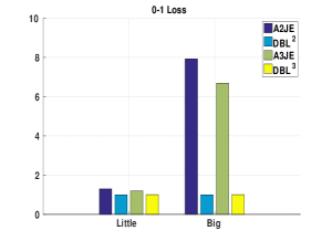
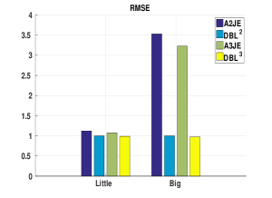
Figure 3: Geometric mean of 0-1 Loss (Left), RMSE (Right) performance of $\text{DBL}^{2}$, A2JE, $\text{DBL}^{3}$ and A3JE for Little and Big datasets.

It can be seen that $\text{DBL}^{n}$ has a lower averaged 0-1 Loss and RMSE than AnJE. This difference is substantial when comparing on Big datasets. The training and classification time of AnJE is, however, substantially lower than $\text{DBL}^{n}$ as can be seen from Figure 4. This is to be expected as $\text{DBL}^{n}$ adds discriminative training to AnJE and uses twice the number of parameters at classification time.

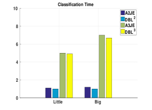
Figure 4: Geometric mean of Training Time (Left), Classification Time (Right) of $\text{DBL}^{2}$, A2JE, $\text{DBL}^{3}$ and A3JE for All and Big datasets.

6.2 $\text{DBL}^{n}$ vs. AnDE

A W-D-L comparison for 0-1 Loss, RMSE, bias and variance results of the two $\text{DBL}^{n}$ models relative to the corresponding AnDE models are presented in Table 3. We compare $\text{DBL}^{2}$ with A1DE and $\text{DBL}^{3}$ with A2DE only. It can be seen that $\text{DBL}^{n}$ has significantly lower bias and significantly higher variance variance than AnDE models. Recently, AnDE models have been proposed as a fast and effective Bayesian classifiers when learning from large quantities of data (Zaidi and Webb, 2012). These bias-variance results make $\text{DBL}^{n}$ a suitable alternative to AnDE when dealing with big data. The 0-1 Loss and RMSE results (with exception of RMSE comparison of $\text{DBL}^{3}$ vs. A2DE) are similar.

	$\text{DBL}^{2}$ vs. A1DE		$\text{DBL}^{3}$ vs. A2DE
	W-D-L	$p$	W-D-L	$p$
	Little Datasets
Bias	65/3/7	$<$0.001	53/5/17	$<$0.001
Variance	21/5/49	0.001	26/5/44	0.041
0-1 Loss	42/4/29	0.1539	39/3/33	0.556
RMSE	30/1/44	0.130	22/1/52	$<$0.001
	Big Datasets
0-1 Loss	8/0/0	0.007	7/0/1	0.073
RMSE	7/0/1	0.073	6/0/2	0.289

Table 3: Win-Draw-Loss: $\text{DBL}^{2}$ vs. A1DE and $\text{DBL}^{3}$ vs A2DE. $p$ is two-tail binomial sign test. Results are significant if $p\leq 0.05$.

Normalized 0-1 Loss and RMSE are shown in Figure 5. It can be seen that the $\text{DBL}^{n}$ models have lower 0-1 Loss and RMSE than the corresponding AnDE models.

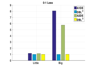
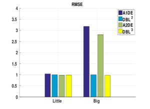
Figure 5: Geometric mean of 0-1 Loss (Left) and RMSE (Right) performance of $\text{DBL}^{2}$, A1DE, $\text{DBL}^{3}$ and A2DE for Little and Big datasets.

A comparison of the training time of $\text{DBL}^{n}$ and AnDE is given in Figure 6. As expected, due to its additional discriminative learning, $\text{DBL}^{n}$ requires substantially more training time than AnDE. However, AnDE does not share such a consistent advantage with respect to classification time, the relativities depending on the dimensionality of the data. For high-dimensional data the large number of permutations of attributes that AnDE must consider results in greater computation.

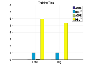
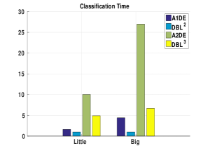
Figure 6: Geometric mean of Training Time (Left), Classification Time (Right) of $\text{DBL}^{2}$, A1DE, $\text{DBL}^{3}$ and A2DE for All and Big datasets.

6.3 $\text{DBL}^{n}$ vs. $\text{LR}^{n}$

In this section, we will compare the two $\text{DBL}^{n}$ models with their equivalent $\text{LR}^{n}$ models. As discussed before, we expect to see similar bias-variance profile and a similar classification performance as the two models are re-parameterization of each other.

We compare the two parameterizations in terms of the scatter of their 0-1 Loss and RMSE values on Little datasets in Figure 7, 9 respectively, and on Big datasets in Figure 8, 10 respectively. It can be seen that the two parameterizations (with an exception of one dataset, that is: wall-following) have a similar spread of 0-1 Loss and RMSE values for both $n=2$ and $n=3$.

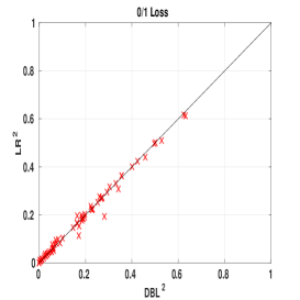
Figure 7: Comparative scatter of 0-1 Loss of $\text{DBL}^{2}$ and $\text{LR}^{2}$ (Left) and $\text{DBL}^{3}$ and $\text{LR}^{3}$ (Right) for Little datasets.

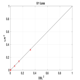
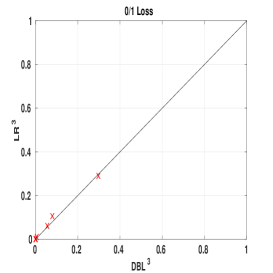
Figure 8: Comparative scatter of 0-1 Loss of $\text{DBL}^{2}$ and $\text{LR}^{2}$ (Left) and $\text{DBL}^{3}$ and $\text{LR}^{3}$ (Right) for Big datasets.

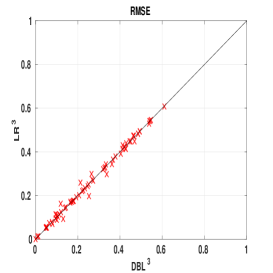
Figure 9: Comparative scatter of RMSE of $\text{DBL}^{2}$ and $\text{LR}^{2}$ (Left) and $\text{DBL}^{3}$ and $\text{LR}^{3}$ (Right) for Little datasets.

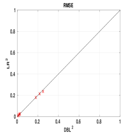
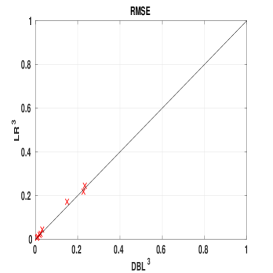
Figure 10: Comparative scatter of RMSE of $\text{DBL}^{2}$ and $\text{LR}^{2}$ (Left) and $\text{DBL}^{3}$ and $\text{LR}^{3}$ (Right) for Big datasets.

The comparative scatter of the number of iterations each parameterization takes to converge is shown in Figure 11 and 12 for Little and Big datasets respectively. It can be seen that the number of iterations for $\text{DBL}^{n}$ are far fewer than $\text{LR}^{n}$. With a similar spread of 0-1 Loss and RMSE values, it is very encouraging to see that $\text{DBL}^{n}$ converges in far fewer iterations.

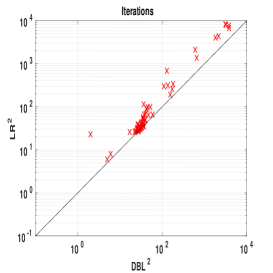
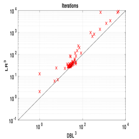
Figure 11: Comparative scatter of number of iterations of $\text{DBL}^{2}$ and $\text{LR}^{2}$ (Left) and $\text{DBL}^{3}$ and $\text{LR}^{3}$ (Right) for Little datasets.

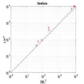
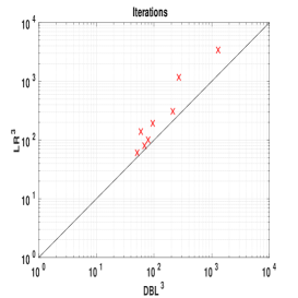
Figure 12: Comparative scatter of iterations of $\text{DBL}^{2}$ and $\text{LR}^{2}$ (Left) and $\text{DBL}^{3}$ and $\text{LR}^{3}$ (Right) for Big datasets.

The number of iterations to converge plays a major part in determining an algorithm’s training time. The training time of the two parameterizations is shown in Figure 13 and 14 for Little and Big datasets, respectively. It can be seen that $\text{DBL}^{n}$ models are much faster than equivalent $\text{LR}^{n}$ models.

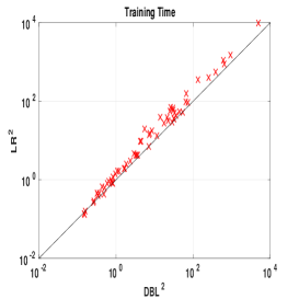
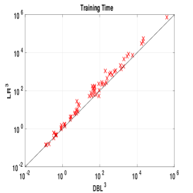
Figure 13: Comparative scatter of Training time of $\text{DBL}^{2}$ and $\text{LR}^{2}$ (Left) and $\text{DBL}^{3}$ and $\text{LR}^{3}$ (Right) for Little datasets.

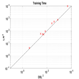
Figure 14: Comparative scatter of Training time of $\text{DBL}^{2}$ and $\text{LR}^{2}$ (Left) and $\text{DBL}^{3}$ and $\text{LR}^{3}$ (Right) for Big datasets.

A comparison of rate of convergence of Negative-Log-Likelihood (NLL) of $\text{DBL}^{2}$ and $\text{LR}^{2}$ parameterization on some sample datasets is shown in Figure 15. It can be seen that, $\text{DBL}^{2}$ has a steeper curve, asymptoting to its global minimum much faster. For example, on almost all datasets, one can see that $\text{DBL}^{2}$ follows a steeper, hence more desirable, path toward convergence. This is extremely advantageous when learning from very few iterations (for example, when learning using Stochastic Gradient Descent based optimization) and, therefore, is a desirable property for scalable learning.

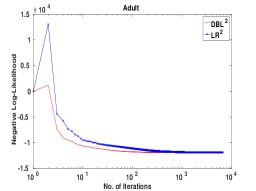
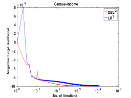
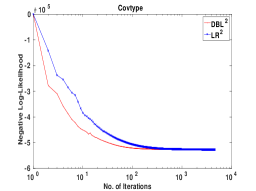
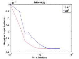
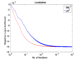
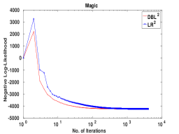
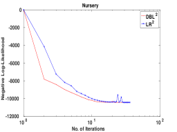
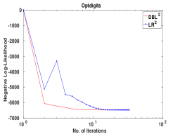
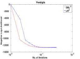
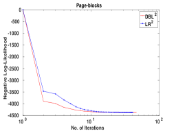
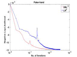
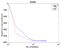
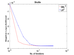
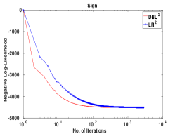
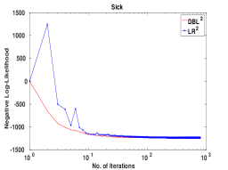
Figure 15: Comparison of rate of convergence of $\text{DBL}^{2}$ and $\text{LR}^{2}$ on several datasets. The X-axis (No. of iterations) is on log scale.

A similar trend can be seen in Figure 16 for $\text{DBL}^{3}$ and $\text{LR}^{3}$.

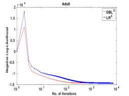
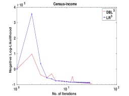
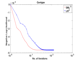
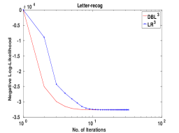
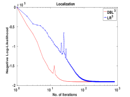
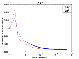
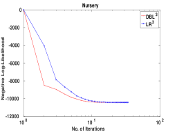
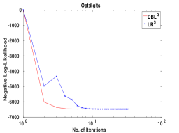
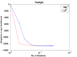
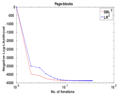
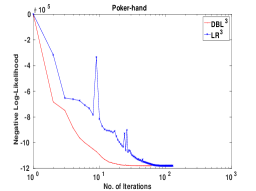
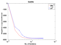
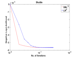
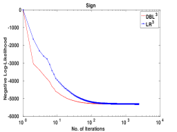
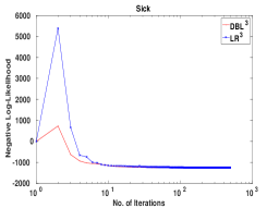
Figure 16: Comparison of rate of convergence of $\text{DBL}^{3}$ and $\text{LR}^{3}$ on several datasets. The X-axis (No. of iterations) is on log scale.

Finally, let us present some comparison results about the speed of convergence of $\text{DBL}^{n}$ vs. $\text{LR}^{n}$ as we increase $n$. In Figure 17, we compare the convergence for $n=1$, $n=2$ and $n=3$ on the sample Localization dataset. It can be seen that the improvement that $\text{DBL}^{n}$ provides over $\text{LR}^{n}$ gets better as we go to deeper structures, i.e., as $n$ becomes larger. The similar behaviour was observed for several datasets and, although studying rates of convergence is a complicated matter and is outside the scope of this work, we anticipate this phenomenon to be an interesting venue of investigation for future work.

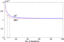
Figure 17: Compared rates of convergence of $\text{DBL}^{n}$ vs. $\text{LR}^{n}$, for $n=1,2,3$ on the sample Localization dataset. Y-axis is the negative log-likelihood.

6.4 $\text{DBL}^{n}$ vs. Random Forest

The two $\text{DBL}^{n}$ models are compared in terms of W-D-L of 0-1 Loss, RMSE, bias and variance with Random Forest in Table 4. On Little datasets, it can be seen that $\text{DBL}^{n}$ has significantly lower bias than RF. The variance of $\text{DBL}^{3}$ is significantly higher than RF, whereas, difference in the variance is not significant for $\text{DBL}^{2}$ and RF. 0-1 Loss results of $\text{DBL}^{n}$ and RF are similar. However, RF has better RMSE results than $\text{DBL}^{n}$ on Little datasets. On Big datasets, $\text{DBL}^{n}$ wins on majority of datasets in terms of 0-1 Loss and RMSE.

	$\text{DBL}^{2}$ vs. RF		$\text{DBL}^{3}$ vs. RF
	W-D-L	$p$	W-D-L	$p$
	Little Datasets
Bias	51/3/21	$<$0.001	52/2/21	$<$0.001
Variance	33/3/39	0.556	28/5/42	0.119
0-1 Loss	40/3/32	0.409	37/3/35	0.906
RMSE	26/1/48	0.014	27/1/47	0.026
	Big Datasets
0-1 Loss	5/0/3	0.726	6/0/2	0.289
RMSE	5/0/3	0.726	5/0/3	0.726

Table 4: Win-Draw-Loss: $\text{DBL}^{2}$ vs. RF and $\text{DBL}^{3}$ vs RF. $p$ is two-tail binomial sign test. Results are significant if $p\leq 0.05$.

The averaged 0-1 Loss and RMSE results are given in Figure 18. It can be seen that $\text{DBL}^{2}$, $\text{DBL}^{3}$ and RF have similar 0-1 Loss and RMSE across Little datasets. However, on Big datasets, the lower bias of $\text{DBL}^{n}$ results in much lower error than RF in terms of both 0-1 Loss and RMSE. These averaged results also corroborate with the W-D-L results in Table 4, showing $\text{DBL}^{n}$ to be a less biased model than RF.

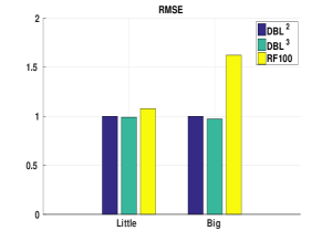
Figure 18: Geometric mean of 0-1 Loss (Left) and RMSE (Right) performance of $\text{DBL}^{2}$, $\text{DBL}^{3}$ and RF for Little and Big datasets.

The comparison of training and classification time of $\text{DBL}^{n}$ and RF is given in Figure 19. It can be seen that $\text{DBL}^{n}$ models are worst than RF in terms of the training time but better in terms of classification time.

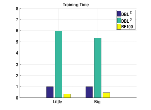
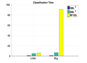
Figure 19: Geometric average of Training Time (Left), Classification Time (Right) of $\text{DBL}^{2}$, $\text{DBL}^{3}$ and RF for Little and Big datasets.

7 Conclusion and Future Work

We have presented an algorithm for deep broad learning. DBL consists of parameters that are learned using both generative and discriminative training. To obtain the generative parameterization for DB, we first developed AnJE, a generative counter-part of higher-order logistic regression. We showed that $\text{DBL}^{n}$ and $\text{LR}^{n}$ learn equivalent models, but that $\text{DBL}^{n}$ is able to exploit the information gained generatively to effectively precondition the optimization process. $\text{DBL}^{n}$ converges in fewer iterations, leading to its global minimum much more rapidly, resulting in faster training time. We also compared $\text{DBL}^{n}$ with the equivalent AnJE and AnDE models and showed that $\text{DBL}^{n}$ has lower bias than both AnJE and AnDE models. We compared $\text{DBL}^{n}$ with state of the art classifier Random Forest and showed that $\text{DBL}^{n}$ models are indeed lower biased than RF and on bigger datasets $\text{DBL}^{n}$ often obtains lower 0-1 loss than RF.

There are a number of exciting new directions for future work.

• We have showed that $\text{DBL}^{n}$ is a low bias classifier with minimal tuning parameters and has the ability to handle multiple classes. The obvious extension is to make it out-of-core. We argue that $\text{DBL}^{n}$ is greatly suited for stochastic gradient descent based methods as it can converge to global minimum very quickly.

• It may be desirable to utilize a hierarchical DBL, such that $h\text{DBL}^{n}=\{\text{DBL}^{1}\ldots\text{DBL}^{n}\}$, incorporating all the parameters up till $n$. This may be useful for smoothing the parameters. For example, if a certain interaction does not occur in the training data, at classification time one can resort to lower values of $n$.

• In this work, we have constrained the values of $n$ to two and three. Scaling-up $\text{DBL}^{n}$ to higher values of $n$ is greatly desirable. One can exploit the fact that many interactions at higher values of $n$ will not occur in the data and hence can develop sparse implementations of $\text{DBL}^{n}$ models.

• Exploring other objective functions such as Mean-Squared-Error or Hinge Loss can result in improving the performance and has been left as a future work.

• The preliminary version of DBL that we have developed is restricted to categorical data and hence requires that numeric data be discretized. While our results show that this is often highly competitive with random forest using local cut-points, on some datasets it is not. In consequence, there is much scope for investigation of deep broad techniques for numeric data.

• DBL presents a credible path towards deep broad learning for big data. We have demonstrated very competitive error on big data and expect future refinements to deliver even more efficient and effective outcomes.

8 Code and Datasets

Code with running instructions can be download from https://www.dropbox.com/sh/iw33mgcku9m2quc/AABXwYewVtm0mVE6KoyMPEVFa?dl=0.

9 Acknowledgments

This research has been supported by the Australian Research Council (ARC) under grants DP140100087, DP120100553, DP140100087 and Asian Office of Aerospace Research and Development, Air Force Office of Scientific Research under contracts FA2386-12-1-4030, FA2386-15-1-4017 and FA2386-15-1-4007.

A Detailed Results

In this appendix, we compare the 0-1 Loss and RMSE results of $\text{DBL}^{n}$, AnDE and RF. The goal here is to assess the performance of each model on Big datasets. Therefore, results on 8 big datasets are reported only in Table 5 and 6 for 0-1 Loss and RMSE respectively. We also compare results with AnJE. Note A1JE is naive Bayes. Also $\text{DBL}^{1}$ results are also compared. Note, $\text{DBL}^{1}$ is WANBIA-C (Zaidi et al., 2013).

The best results are shown in bold font.

Table 5: 0-1 Loss values of A1JE, A2JE, A3JE, A1DE, A2DE, $\text{DBL}^{1}$, $\text{DBL}^{2}$, $\text{DBL}^{3}$, RF and RF (numeric) on Big datasets.

	Locali-zation	Poker-hand	Census-income	Covtype	Kddcup	MITFa-ceSetA	MITFa-ceSetB	MITFa-ceSetC
A1JE	0.4938	0.4988	0.2354	0.3143	0.0091	0.0116	0.0268	0.0729
A2JE	0.3653	0.0763	0.2031	0.2546	0.0061	0.0106	0.0239	0.0630
A3JE	0.2813	0.0763	0.1674	0.1665	0.0053	0.0096	0.0215	0.0550
A1DE	0.3584	0.4640	0.0986	0.2387	0.0025	0.0124	0.0322	0.0417
A2DE	0.2844	0.1348	0.0682	0.1552	0.0023	0.0105	0.0325	0.0339
$\text{DBL}^{1}$	0.4586	0.4988	0.0433	0.2576	0.0017	0.0012	0.0047	0.0244
$\text{DBL}^{2}$	0.3236	0.0021	0.0686	0.1381	0.0014	0.0002	0.0007	0.0007
$\text{DBL}^{3}$	0.2974	0.0056	0.0557	0.0797	0.0013	0.0001	0.0005	0.0005
RF	0.2976	0.0687	0.0494	0.0669	0.0015	0.0012	0.0022	0.0013

Table 6: RMSE values of A1JE, A2JE, A3JE, A1DE, A2DE, $\text{DBL}^{1}$, $\text{DBL}^{2}$, $\text{DBL}^{3}$ and RF on Big datasets.

	Locali-zation	Poker-hand	Census-income	Covtype	Kddcup	MITFa-ceSetA	MITFa-ceSetB	MITFa-ceSetC
A1JE	0.2386	0.2382	0.4599	0.2511	0.0204	0.1053	0.1607	0.2643
A2JE	0.2115	0.1924	0.4231	0.2256	0.0170	0.1006	0.1516	0.2455
A3JE	0.1972	0.1721	0.3812	0.1857	0.0160	0.0954	0.1436	0.2293
A1DE	0.2090	0.2217	0.2780	0.2174	0.0103	0.1079	0.1746	0.1989
A2DE	0.1890	0.2044	0.2269	0.1779	0.0098	0.0983	0.1745	0.1530
$\text{DBL}^{1}$	0.2330	0.2382	0.1807	0.2254	0.0072	0.0347	0.0602	0.1360
$\text{DBL}^{2}$	0.2179	0.1970	0.250	0.1802	0.0068	0.0123	0.0248	0.0257
$\text{DBL}^{3}$	0.2273	0.0323	0.2332	0.1494	0.0065	0.0105	0.0198	0.0241
RF	0.1939	0.1479	0.1928	0.1336	0.0072	0.0296	0.0484	0.0651

References

- Boyd and Vandenberghe (2008) S Boyd and L Vandenberghe. Convex Optimization. Cambridge Unversity Press, 2008.
- Brain and Webb (2002) Damien Brain and Geoffrey I. Webb. The need for low bias algorithms in classification learning from small data sets. In PKDD, pages 62–73, 2002.
- Breiman (2001) L Breiman. Random forests. Machine Learning, 45:5–32, 2001.
- Byrd et al. (1995) R.H Byrd, P Lu, and J Nocedal. A limited memory algorithm for bound constrained optimization. SIAM Journal on Scientific and Statistical Computing, 16(5):1190–1208, 1995.
- Fayyad and Irani (1992) Usama M Fayyad and Keki B Irani. On the handling of continuous-valued attributes in decision tree generation. Machine Learning, 8(1):87–102, 1992.
- Frank and Asuncion (2010) A Frank and A Asuncion. UCI machine learning repository, 2010. URL http://archive.ics.uci.edu/ml.
- Ganz and Reinsel (2012) J. Ganz and D. Reinsel. The Digital Universe Study, 2012.
- Greiner and Zhou (2002) R. Greiner and W. Zhou. Structural extension to logistic regression: Discriminative paramter learning of belief net classifiers. In AAAI, 2002.
- Greiner et al. (2004) Russell Greiner, Wei Zhou, Xiaoyuan Su, and Bin Shen. Structural extensions to logistic regression: Discriminative parameter learning of belief net classifiers. Journal of Machine Learning Research, 2004.
- Langford et al. (2007) J. Langford, L. Li, and A. Strehl. Vowpal wabbit online learning project, 2007.
- Martinez et al. (2015) S. Martinez, A. Chen, G. I. Webb, and N. A. Zaidi. Scalable learning of bayesian network classifiers. Journal of Machine Learning Research, 2015.
- Pernkopf and Bilmes (2005) F. Pernkopf and J. Bilmes. Discriminative versus generative parameter and structure learning of bayesian network classifiers. In ICML, 2005.
- Pernkopf and Wohlmayr (2009) F. Pernkopf and M. Wohlmayr. On discriminative parameter learning of bayesian network classifiers. In ECML PKDD, 2009.
- Roos et al. (2005) T Roos, H Wettig, P Grünwald, P Myllymäki, and H Tirri. On discriminative Bayesian network classifiers and logistic regression. Machine Learning, 59(3):267–296, 2005.
- Sahami (1996) M Sahami. Learning limited dependence Bayesian classifiers. In Proceedings of the Second International Conference on Knowledge Discovery and Data Mining, pages 334–338, Menlo Park, CA, 1996. AAAI Press.
- Su et al. (2008) J. Su, H. Zhang, C. Ling, and S. Matwin. Discriminative parameter learning for bayesian networks. In ICML, 2008.
- Webb et al. (2005) G I. Webb, J Boughton, and Z Wang. Not so naive Bayes: Averaged one-dependence estimators. Machine Learning, 58(1):5–24, 2005.
- Webb et al. (2011) Geoffrey I. Webb, Janice Boughton, Fei Zheng, Kai Ming Ting, and Houssam Salem. Learning by extrapolation from marginal to full-multivariate probability distributions: decreasingly naive Bayesian classification. Machine Learning, pages 1–40, 2011. ISSN 0885-6125. URL http://dx.doi.org/10.1007/s10994-011-5263-6. 10.1007/s10994-011-5263-6.
- Zaidi and Webb (2012) N. A. Zaidi and G. I. Webb. Fast and efficient single pass Bayesian learning. In Proceedings of the 17th Pacific-Asia Conference on Knowledge Discovery and Data Mining (PAKDD), 2012.
- Zaidi et al. (2013) N. A. Zaidi, J. Cerquides, M. J Carman, and G. I. Webb. Alleviating naive Bayes attribute independence assumption by attribute weighting. Journal of Machine Learning Research, 14:1947–1988, 2013.
- Zaidi et al. (2014) N. A. Zaidi, M. J Carman, J. Cerquides, and G. I. Webb. Naive-bayes inspired effective pre-conditioners for speeding-up logistic regression. In IEEE International Conference on Data Mining, 2014.
- Zhu et al. (1997) C. Zhu, R. H. Byrd, and J. Nocedal. LBFGSB, fortran routines for large scale bound constrained optimization. ACM Transactions on Mathematical Software, 23(4):550–560, 1997.