Adaptive Control of Uncertain Pure-feedback Nonlinear Systems

Abstract

A novel adaptive control approach is proposed to solve the globally asymptotic state stabilization problem for uncertain pure-feedback nonlinear systems which can be transformed into the pseudo-affine form. The pseudo-affine pure-feedback nonlinear system under consideration is with non-linearly parameterised uncertainties and possibly unknown control coefficients. Based on the parameter separation technique, a backstepping controller is designed by adopting the adaptive high gain idea. The rigorous stability analysis shows that the proposed controller could guarantee, for any initial system condition, boundedness of the closed-loop signals and globally asymptotic stabilization of the state. A numerical and a realistic examples are employed to demonstrate the effectiveness of the proposed control method.

1 Introduction

During the past several decades, control of nonlinear systems has received considerable attention and a series of powerful control methods have been proposed, such as sliding mode control (Slotine and Li, 1991), feedback linearization (Sastry and Isidori, 1989), backstepping (Kanellakopoulos, Kokotovic, and Morse, 1991), and so on. Among these methods, the backstepping technique, which is a constructive, recursive, Lyapunov-based control design approach, is one of the most popular control design tools to deal with a large class of nonlinear systems with uncertainties, especially with unmatched uncertainties. Nonlinear systems using the backstepping technique are of lower triangular form which can be broadly classified into two kinds: strict-feedback form and pure-feedback form. In the case of strict-feedback systems, a great deal of progress has been achieved to develop backstepping controllers. It is first proposed for nonlinear systems with linearly parameterized uncertainties (Kanellakopoulos, Kokotovic, and Morse, 1991; Krstic, Kanellakopoulos, and Kokotovid, 1995), and then extended to handle non-linearly parameterized uncertainties (Lin and Qian, 2002a, b; Niu, Lam, Wang, and Ho, 2005). By introducing Nussbaum functions, it is also applied to nonlinear systems with unknown control directions (Ye, 1999). The relevant engineering applications have also been widely discussed, for example, from wheeled mobile robots (Mnif and Yahmadi, 2005) to aircrafts (Lungu and Lungu, 2013) to spacecrafts (Ali, Radice, and Kim, 2010).

Compared with this progress, relatively fewer results are available for control of pure-feedback systems. Pure-feedback systems, which have no affine appearance of the state variables to be used as virtual controls and/or the actual control, is more representative than strict-feedback systems. Many practical systems are of pure-feedback form, such as aircraft control systems (Hunt and Mayer, 1997), biochemical processes (Krstic, Kanellakopoulos, and Kokotovid, 1995), mechanical systems (Ferrara and Giacomini, 2000), and so on. Cascade and non-affine properties of pure-feedback systems make it rather difficult to find explicit virtual controls and the actual control. Therefore, control of non-affine pure-feedback nonlinear systems is a meaningful and challenging issue and has become a hot topic in the control field in recent years (See Liu (2016); Liu and Tong (2016) and references therein). Most of these results are approximation-based approaches which fully exploit the universal approximation ability of neural networks or fuzzy logic systems. By utilizing the Mean Value Theorem, the original non-affine system is transformed to the quasi-affine form. Subsequently, the backstepping technique is employed for the control design. Generally speaking, it is difficult to obtain the explicit expressions of the ideal virtual or actual controllers although their existence is guaranteed by the Implicit Function Theorem. Hence, to approximate them, estimators are constructed based on fuzzy logic systems (Gao, Sun, and Xu, 2013; Li, Tong, and Li, 2015; Yu, 2013; Zhang, Wen, and Zhu, 2010) or neural networks (Shen, Shi, Zhang, and Lim, 2014; Sun, Wang, Li, and Peng, 2013; Wang, Hill, Ge, and Chen, 2006; Wang, Liu, and Shi, 2011; Wang, Chen, and Lin, 2013). In Yoo (2012) and Gao, Sun, and Liu (2012), the singular perturbation theory is also employed to estimate the ideal controllers.

Approximation-based approaches may suffer some problems. Take the approaches based on neural networks for example. When the number of the neural network nodes increases to improve the approximation ability, the number of adjustable parameters will become enormous. Accordingly, the online learning time will become very large (Liu and Tong, 2016). In addition, the obtained results usually hold non-globally. To avoid suchlike problems, some approximation-free approaches are proposed recently. In Liu (2014), a backstepping control algorithm is proposed for a class of pure-feedback nonlinear systems by viewing $f_{i}(\bar{x}_{i+1})$ in stead of $x_{i+1}$ as the virtual control variable and by adding anintegrator. This result is further extended to the case where there exist linearly parameterised uncertainties (Liu, 2016). In Liu and Tong (2016), by adopting the barrier Lyapunov function technique, an adaptive control technique is developed for a class of pure-feedback systems with linearly parameterised uncertainties and full state constraints.

In this paper, the globally asymptotic state stabilization (GASS) problem is considered for a class of pure-feedback systems which can be written into the pseudo-affine form. The pseudo-affine pure-feedback system under consideration has non-linearly parameterised uncertainties and possibly unknown control coefficients. For this kind of systems, if the lower bound of every control coefficient is exactly known, the GASR problem can be solved by the non-smooth or the smooth control schemes given in Lin and Qian (2002a, b). When their lower bounds are unknown, a possible way is to adopt and improve the adaptive control approach proposed in Sun and Liu (2007). If so, $2n$ adaptive laws are needed to estimate the unknown parameters. In this paper, motivated by the work in Ye (1999) and the high gain idea given in Lei and Lin (2006), a novel adaptive backstepping controller is proposed based on the parameter separation technique (Lin and Qian, 2002a, b). In the proposed method, only $n$ adaptive laws are needed. Since no estimators are needed to approximate the ideal controllers, drawbacks of the approximation-based approaches can be avoided. The rigorous stability analysis shows that the proposed controller could guarantee bounded closed-loop signals and globally asymptotic state stabilization.

2 Problem Formulation

Consider pure-feedback nonlinear systems which can be written into the following pseudo-affine form

$$\left\{\begin{array}[]{l}\dot{x}_{i}=\varphi_{i}(\bar{x}_{i},\theta)+g_{i}(\bar{x}_{i+1},\theta)x_{i+1},(i=1,\cdots,n-1)\\ \dot{x}_{n}=\varphi_{n}(x,\theta)+g_{n}(x,\theta,u)u\\ y=x_{1}\end{array}\right.$$ (4)

where $x=[\begin{array}[]{ccc}x_{1}&\cdots&x_{n}\end{array}]^{\mathrm{T}}$ is the state, $\bar{x}_{i}=[\begin{array}[]{ccc}x_{1}&\cdots&x_{i}\end{array}]^{\mathrm{T}}$, $u$ is the input, $y$ is the output, $\theta:\Re_{\geq 0}\rightarrow\Re^{m}$ is a bounded, uncertain time-varying piecewise continuous parameter or disturbance vector, $\varphi_{i}:\Re^{i+m}\rightarrow\Re$ and $g_{i}:\Re^{i+1+m}\rightarrow\Re$ are $\mathcal{C}^{1}$ functions, and $\varphi_{i}(0_{i\times 1},\theta)=0$. For notational convenience, we introduce $x_{n+1}:=u$.

Remark 1.

For general pure-feedback systems

$$\left\{\begin{array}[]{l}\dot{x}_{i}=f_{i}(\bar{x}_{i+1},\theta),(i=1,\cdots,n-1)\\ \dot{x}_{n}=f_{n}(x,\theta,u)\end{array}\right.$$ (5)

where $f_{i}:\Re^{i+1+s}\rightarrow\Re$ are $\mathcal{C}^{2}$ functions satisfying $f_{i}(0_{i\times 1},\theta,0)=0$, by the Mean Value Theorem, we have

$$f_{i}(\bar{x}_{i+1},\theta)=f_{i}(\bar{x}_{i},0,\theta)+\frac{\partial f_{i}(\bar{x}_{i},\lambda_{i}x_{i+1},\theta)}{\partial x_{i+1}}x_{i+1}$$ (6)

where $\lambda_{i}\in(0,1)$ and is a constant or a $\bar{x}_{i+1}$-dependent variable. Define $\varphi_{i}(\bar{x}_{i},\theta)=f_{i}(\bar{x}_{i},0,\theta)$ and $g_{i}(\bar{x}_{i+1},\theta)=\frac{\partial f_{i}(\bar{x}_{i},\lambda_{i}x_{i+1},\theta)}{\partial x_{i+1}}$. It is easy to know that $\varphi_{i}$ and $g_{i}$ are $\mathcal{C}^{1}$ functions, and $\varphi_{i}(0_{i\times 1},\theta)=0$. Hence, system (5) can be transformed to the form of (4).

In this paper, we are interested in the case where $\varphi_{i}$ and $g_{i}$ satisfy the following two assumptions, respectively.

Assumption 1: There exist a set of unknown constants $c_{i}$ and known $\mathcal{C}^{1}$ functions $\rho_{i}:\Re^{i}\rightarrow\Re_{\geq 0}$ such that

$$\left|\varphi_{i}(\bar{x}_{i},\theta)\right|\leq c_{i}\rho_{i}(\bar{x}_{i})\sum_{j=1}^{i}\left|x_{j}\right|,(i=1,\cdots,n)$$ (7)

Assumption 2: The signs of $g_{i}$ are known. Without loss of generality, we assume that they are all positive. In addition, we assume that there exist a set of unknown constants $b_{i}>0$, $B_{i}>0$, and known $\mathcal{C}^{1}$ functions $\phi_{i}:\Re^{i+1}\rightarrow\Re_{>0}$ such that

$$0<b_{i}\leq g_{i}(\bar{x}_{i+1},\theta)\leq B_{i}\phi_{i}(\bar{x}_{i+1}),(i=1,\cdots,n-1)$$ (8)

and $g_{n}(x,\theta,u)\geq b_{n}>0$.

The control problem to be solved is stated as follows.

GASS Problem: Consider the uncertain pure-feedback system (4) under Assumptions 1 and 2. Design a $\mathcal{C}^{1}$ state feedback controller $u$ such that all signals in the resulting closed-loop system are bounded on $[0,\infty)$, furthermore, globally asymptotic stabilization of the state $x$ is achieved, i.e. $\lim_{t\rightarrow\infty}x(t)=0$ for all $x(0)\in\Re^{n}$.

Remark 2.

The condition $g_{i}\geq b_{i}>0$ actually presents a sufficient global controllability condition for system (4). In addition, since $\varphi_{i}(\bar{x}_{i},\theta)$ is a $\mathcal{C}^{1}$ function, according to Nijmeijer and van der (1990), it can be rewritten as $\varphi_{i}(\bar{x}_{i},\theta)=\sum\nolimits_{j=1}^{i}\xi_{ij}(\bar{x}_{i},\theta)x_{j}$ with $\xi_{ij}$ being continuous functions. According to the parameter separation technique introduced in Lin and Qian (2002a) and Lin and Qian (2002b), it is reasonable to assume that, $\forall j=1,\cdots,i$, $\left|\xi_{ij}(\bar{x}_{i},\theta)\right|\leq c_{i}\rho_{i}(\bar{x}_{i})$, which implies that $\left|\varphi_{i}(\bar{x}_{i},\theta)\right|\leq c_{i}\rho_{i}(\bar{x}_{i})\sum\nolimits_{j=1}^{i}\left|x_{j}\right|$, and $g_{i}(\bar{x}_{i+1},\theta)\leq B_{i}\phi_{i}(\bar{x}_{i+1})$, where $c_{i}$ and $B_{i}$ are unknown parameters, and $\rho_{i}$ and $\phi_{i}$ are known smooth functions. In fact, assumptions like Assumptions 1 and 2 are frequently used in the literature, such as Lin and Qian (2002a), Lin and Qian (2002b), Sun and Liu (2007), and so on. It is worth pointing out that the control coefficients $g_{i}$ themselves could be unknown functions under Assumption 2.

3 Main results

In this section, we shall first present an adaptive control scheme, and subsequently we shall prove that it leads to the solution to the GASR problem for system (4).

3.1 Control Scheme

The proposed adaptive control scheme is given in a step-by-step way as follows.

Step 0: Introduce the following coordinate transformation

$$z_{1} = x_{1}$$ (9)

$$z_{i} = x_{i}-\alpha_{i-1},i=2,\cdots,n$$ (10)

where $\alpha_{i},i=1,\cdots,n-1$ are the virtual control laws to be determined. For notational convenience, we introduce $\alpha_{n}:=u$. Virtual control laws $\alpha_{i},i=1,\cdots,n-1$ and the actual control law $\alpha_{n}$ ,i.e., $u$, are constructed as

$$\alpha_{i}(\bar{x}_{i},\bar{k}_{i}) = -\mu_{i}k_{i}\psi_{i}^{2}(\bar{z}_{i},\bar{k}_{i-1})z_{i},(i=1,\cdots,n)$$ (11)

where $k_{i},i=1,\cdots,n$ are update laws given by

$$\dot{k}_{i} = \gamma_{i}\psi_{i}^{2}(\bar{z}_{i},\bar{k}_{i-1})z_{i}^{2}\doteq\omega_{i},k_{i}(0)=k_{i0}\in\Re_{>0}$$ (12)

where $\psi_{i}$ are $\mathcal{C}^{1}$ functions to be determined in the following $i$th step, $\mu_{i}\in\Re_{>0}$ and $\gamma_{i}\in\Re_{>0}$ are design parameters. Roughly speaking, by choosing bigger $\mu_{i}$ and $\gamma_{i}$, the convergence speed of the states can be improved. However, this may lead to larger control magnitude. Therefore, a tradeoff is required when determining these design parameters in applications.

Step 1: Start with

$$\dot{z}_{1} = \dot{x}_{1}=\varphi_{1}+g_{1}x_{2}$$ (13)

Define $V_{1}=\frac{1}{2}z_{1}^{2}$. According to (10)-(12) and Assumptions 1 and 2, the time derivative of $V_{1}$ is such that

$$\dot{V}_{1} = z_{1}\dot{z}_{1}\leq c_{1}\rho_{1}(z_{1})z_{1}^{2}+g_{1}z_{1}(z_{2}+\alpha_{1})$$ (14)

$$\leq -b_{1}\mu_{1}k_{1}\psi_{1}^{2}z_{1}^{2}+c_{1}\rho_{1}(z_{1})z_{1}^{2}+z_{1}^{2}+B_{1}^{2}\phi_{1}^{2}(\bar{x}_{2})z_{2}^{2}$$

Choose $\psi_{1}$ to be any $\mathcal{C}^{1}$ function satisfying

$$\rho_{1}(z_{1})+1\leq\psi_{1}(z_{1})$$ (15)

then

$$\dot{V}_{1} \leq -b_{1}\mu_{1}k_{1}\psi_{1}^{2}z_{1}^{2}+\beta_{1}\psi_{1}^{2}z_{1}^{2}+z_{1}^{2}+\sigma_{1}\phi_{1}^{2}(\bar{x}_{2})z_{2}^{2}$$ (16)

$$= -\frac{1}{\gamma_{1}}b_{1}\mu_{1}k_{1}\dot{k}_{1}+\frac{1}{\gamma_{1}}\beta_{1}\dot{k}_{1}+z_{1}^{2}+\sigma_{1}\phi_{1}^{2}(\bar{z}_{2},k_{1})z_{2}^{2}$$

where $\beta_{1}=c_{1}$ and $\sigma_{1}=B_{1}^{2}$ are unknown constants.

Step i $(2\leq i\leq n)$: The derivative of $z_{i}$ is

$$\dot{z}_{i} = \dot{x}_{i}-\dot{\alpha}_{i-1}=\varphi_{i}+g_{i}x_{i+1}-\sum_{j=1}^{i-1}\left[\frac{\partial\alpha_{i-1}}{\partial x_{j}}\left(\varphi_{j}+g_{j}x_{j+1}\right)+\frac{\partial\alpha_{i-1}}{\partial k_{j}}\omega_{j}\right]$$ (17)

Define $V_{i}=\frac{1}{2}z_{i}^{2}$. Bearing (10)-(12) and Assumptions 1 and 2 in mind, we can obtain

$$\dot{V}_{i} = z_{i}\dot{z}_{i}=z_{i}\varphi_{i}+g_{i}z_{i}x_{i+1}-z_{i}\sum_{j=1}^{i-1}\left[\frac{\partial\alpha_{i-1}}{\partial x_{j}}\left(\varphi_{j}+g_{j}x_{j+1}\right)+\frac{\partial\alpha_{i-1}}{\partial k_{j}}\omega_{j}\right]$$ (18)

$$\leq g_{i}z_{i}x_{i+1}+c_{i}\rho_{i}(\bar{x}_{i})\left|z_{i}\right|\sum_{j=1}^{i}\left|x_{j}\right|$$

$$+\left|z_{i}\right|\sum_{j=1}^{i-1}\left[\left|\frac{\partial\alpha_{i-1}}{\partial x_{j}}\right|\left(c_{j}\rho_{j}(\bar{x}_{j})\sum_{l=1}^{j}\left|x_{l}\right|+g_{j}\left|x_{j+1}\right|\right)+\gamma_{j}\left|\frac{\partial\alpha_{i-1}}{\partial k_{j}}\right|\psi_{j}^{2}(\bar{z}_{j},\bar{k}_{j-1})z_{j}^{2}\right]$$

$$\leq g_{i}z_{i}x_{i+1}+\vartheta_{i}\left|z_{i}\right|\rho_{i}(\bar{x}_{i})\sum_{j=1}^{i}\left|x_{j}\right|$$

$$+\vartheta_{i}\left|z_{i}\right|\sum_{j=1}^{i-1}\left[\left|\frac{\partial\alpha_{i-1}}{\partial x_{j}}\right|\left(\rho_{j}(\bar{x}_{j})\sum_{l=1}^{j}\left|x_{l}\right|+\phi_{j}(\bar{x}_{j+1})\left|x_{j+1}\right|\right)+\gamma_{j}\left|\frac{\partial\alpha_{i-1}}{\partial k_{j}}\right|\psi_{j}^{2}(\bar{z}_{j},\bar{k}_{j-1})z_{j}^{2}\right]$$

where $\vartheta_{i}=\max(1,c_{1},c_{2},\cdots,c_{i},B_{1},\cdots,B_{i})$. According to (10) and (11), we have that, for $2\leq q\leq i$,

$$\left|x_{q}\right|\leq\left|z_{q}\right|+\mu_{q-1}k_{q-1}\psi_{q-1}^{2}(\bar{z}_{q},\bar{k}_{q-2})\left|z_{q-1}\right|$$ (19)

Hence,

$$\dot{V}_{i}\leq g_{i}z_{i}x_{i+1}+\vartheta_{i}\left|z_{i}\right|\eta_{i}(\bar{z}_{i},\bar{k}_{i-1})\sum_{j=1}^{i}\left|z_{j}\right|$$ (20)

where $\eta_{i}(\bar{z}_{i},\bar{k}_{i-1})$ is a known nonnegative-valued function. Now we choose $\psi_{i}$ to be any $\mathcal{C}^{1}$ function satisfying

$$\psi_{i}(\bar{z}_{i},\bar{k}_{i-1})\geq\eta_{i}(\bar{z}_{i},\bar{k}_{i-1})+\phi_{i-1}(\bar{z}_{i},\bar{k}_{i-1})+1$$ (21)

Then, we can obtain

$$\dot{V}_{i} \leq g_{i}z_{i}(z_{i+1}+\alpha_{i})+\vartheta_{i}\left|z_{i}\right|\eta_{i}(\bar{z}_{i},\bar{k}_{i-1})\sum_{j=1}^{i}\left|z_{j}\right|$$ (22)

$$\leq -b_{i}\mu_{i}k_{i}\psi_{i}^{2}(\bar{z}_{i},\bar{k}_{i-1})z_{i}^{2}+z_{i}^{2}+\sigma_{i}\phi_{i}^{2}(\bar{x}_{i+1})z_{i+1}^{2}+i\vartheta_{i}^{2}\psi_{i}^{2}(\bar{x}_{i},\bar{k}_{i-1})z_{i}^{2}+\sum_{j=1}^{i}z_{j}^{2}$$

$$\leq -b_{i}\mu_{i}k_{i}\psi_{i}^{2}(\bar{z}_{i},\bar{k}_{i-1})z_{i}^{2}+\beta_{i}\psi_{i}^{2}(\bar{z}_{i},\bar{k}_{i-1})z_{i}^{2}+\sigma_{i}\phi_{i}^{2}(\bar{z}_{i+1},\bar{k}_{i})z_{i+1}^{2}+\sum_{j=1}^{i}z_{j}^{2}$$

$$= -\frac{1}{\gamma_{i}}b_{i}\mu_{i}k_{i}\dot{k}_{i}+\frac{1}{\gamma_{i}}\beta_{i}\dot{k}_{i}+\sigma_{i}\phi_{i}^{2}(\bar{z}_{i+1},\bar{k}_{i})z_{i+1}^{2}+\sum_{j=1}^{i}z_{j}^{2}$$

where $z_{n+1}=x_{n+1}-\alpha_{n}=0$, $\beta_{i}=i\vartheta_{i}^{2}+1$ and $\sigma_{i}=B_{i}^{2}$ are unknown constants.

3.2 Stability Analysis

Theorem 1.

Suppose that Assumptions 1 and 2 are satisfied and that the above-proposed design procedure is applied to system (4), then for all $x(0)\in\Re^{n}$ and fixed $k_{i}(0)=k_{i0}>0$, $i=1,\cdots,n$, all signals in the resulting closed-loop system are bounded on $[0,\infty)$, furthermore, $\lim_{t\rightarrow\infty}x(t)=0$ and $\lim_{t\rightarrow\infty}k_{i}(t)=k_{i\infty}\in\Re_{>0}$.

Proof.

Due to the smoothness of the proposed robust control, the solution of the closed-loop system has a maximum interval of existence $[0,t_{f})$ where $t_{f}\in\Re_{>0}$. We will first prove the boundedness of all state variables on the interval $[0,\infty)$, and then prove the convergence of $x(t)$ and $k_{i}(t)$. To this end, we define

$$V=\sum_{i=1}^{n}V_{i}=\frac{1}{2}\sum_{i=1}^{n}z_{i}^{2}\geq 0$$ (23)

It follows from (15), (16), (21), (22) and the fact $z_{n+1}=0$ that

$$\dot{V} = \sum_{i=1}^{n}\dot{V}_{i}\leq-\sum_{i=1}^{n}\frac{1}{\gamma_{i}}b_{i}\mu_{i}k_{i}\dot{k}_{i}+\sum_{i=1}^{n}\frac{1}{\gamma_{i}}\beta_{i}\dot{k}_{i}+\sum_{i=1}^{n-1}\sigma_{i}\phi_{i}^{2}(\bar{z}_{i+1},\bar{k}_{i})z_{i+1}^{2}+\sum_{i=1}^{n}\sum_{j=1}^{i}z_{j}^{2}$$ (24)

$$\leq -\sum_{i=1}^{n}\frac{1}{\gamma_{i}}b_{i}\mu_{i}k_{i}\dot{k}_{i}+\sum_{i=1}^{n}\frac{1}{\gamma_{i}}\beta_{i}\dot{k}_{i}+\sum_{i=1}^{n-1}\sigma_{i}\psi_{i+1}^{2}(\bar{z}_{i+1},\bar{k}_{i})z_{i+1}^{2}+\sum_{i=1}^{n}\sum_{j=1}^{i}\psi_{j}^{2}(\bar{z}_{j},\bar{k}_{j-1})z_{j}^{2}$$

$$\leq -\sum_{i=1}^{n}\frac{1}{\gamma_{i}}b_{i}\mu_{i}k_{i}\dot{k}_{i}+\sum_{i=1}^{n}\frac{1}{\gamma_{i}}\beta_{i}\dot{k}_{i}+\sum_{i=1}^{n-1}\sigma_{i}\frac{1}{\gamma_{i+1}}\dot{k}_{i+1}+\sum_{i=1}^{n}\sum_{j=1}^{i}\frac{1}{\gamma_{j}}\dot{k}_{j}$$

$$\leq -\sum_{i=1}^{n}\frac{1}{\gamma_{i}}b_{i}\mu_{i}k_{i}\dot{k}_{i}+\varepsilon\sum_{i=1}^{n}\frac{1}{\gamma_{i}}\dot{k}_{i}+\varepsilon\sum_{i=1}^{n}\frac{1}{\gamma_{i}}\dot{k}_{i}$$

$$= -\sum_{i=1}^{n}\frac{1}{\gamma_{i}}b_{i}\mu_{i}k_{i}\dot{k}_{i}+2\varepsilon\sum_{i=1}^{n}\frac{1}{\gamma_{i}}\dot{k}_{i}$$

where $\varepsilon=\max\left(\beta_{1},\cdots,\beta_{n},n,n-1+\sigma_{1},\cdots,1+\sigma_{n-1}\right)$ is an unknown constant. Integrating inequality (24) gives, $\forall t\in[0,t_{f})$,

$$V(t) \leq -\frac{1}{2}\sum_{i=1}^{n}\frac{1}{\gamma_{i}}b_{i}\mu_{i}k_{i}^{2}(t)+2\varepsilon\sum_{i=1}^{n}\frac{1}{\gamma_{i}}k_{i}(t)+C_{0}$$ (25)

where $C_{0}$ is a constant depending on initial data. This implies that $k_{i}$ are bounded on $[0,t_{f})$. Otherwise, on taking limit as $t\rightarrow t_{f}$, the right side of the above inequality would diverge to $-\infty$, which would yield a contradiction with $V(t)\geq 0$. It immediately follows from (25) that $V(t)$, and in turn, $z_{i}(t)$ are bounded. According to (9)-(11), $x_{i}(t)$ are bounded. Therefore, all the state variables of the closed-loop system are bounded on the interval $[0,t_{f})$, hence, $t_{f}=\infty$. As a result, the control $u$ which depends on $x_{i}$ and $k_{i}$ is bounded, which means that $\dot{x}_{i}(t)$ is bounded. Furthermore, $\dot{k}_{i}(t)$ is bounded according to (12). Hence, by (13) and (17), $\dot{z}_{i}(t)$ is bounded. Since $k_{i}(t)$ is bounded on $[0,+\infty)$ and $\dot{k}_{i}\geq 0$, there exist constants $k_{i\infty}\in\Re_{>0}$ such that $\lim_{t\rightarrow\infty}k_{i}(t)=k_{i\infty}$. From (15) and (21), we have $\psi_{i}\geq 1$. This, together with (12), implies that $z_{i}^{2}(t)\leq\frac{k_{i}(t)}{\gamma_{i}}$. Thus,

$$\lim_{t\rightarrow\infty}\int\nolimits_{0}^{t}z_{i}^{2}(\tau)\mathrm{d}\tau\leq\lim_{t\rightarrow\infty}\int\nolimits_{0}^{t}\frac{\dot{k}_{i}(\tau)}{\gamma_{i}}\mathrm{d}\tau=\frac{k_{i\infty}-k_{i0}}{\gamma_{i}}$$ (26)

Therefore, by using Barbalat’s Lemma (Tao, 1997; Hou, Duan, and Guo, 2010), we have $\lim_{t\rightarrow\infty}z_{i}(t)=0$, that is, $\lim_{t\rightarrow\infty}z(t)=0$. Consequently, from (9)-(11) and the boundedness of $k_{i}(t)$, we can get that $\lim_{t\rightarrow\infty}x(t)=0$. This completes the proof. ∎

Remark 3.

The proposed control algorithm is also available if $\phi_{i}$ and $g_{i}$ are functions of $x$. Of course, $\rho_{i}$ and $\phi_{i}$ are still functions of $\bar{x}_{i}$ and $\bar{x}_{i+1}$, respectively. In this case, system (4) is beyond the lower triangular form.

Remark 4.

The intuitive explanation of the proposed method is given as follows. As long as $z_{i}\neq 0$, $k_{i}$ will keep on growing. When $k_{i}$ become large enough, the uncertainties will be dominated completely and $z_{i}$ will converge to zero eventually. In practical applications, if necessary, we could add the following modification to the update law (12): $\dot{k}_{i}=0$ if $|z_{i}|<\delta$, where $\delta$ characterizes the tolerable error range. In this case, if $|z_{i}|\geq\delta$, $k_{i}$ will grow. When $k_{i}$ become large enough, the uncertainties will be dominated fully and $|z_{i}|$ will decrease ultimately and be kept within the tolerable range. This way could prevent $k_{i}$ from increasing unboundedly and reinforce the closed-loop robustness.

4 Examples

In this section, we will give two examples to show the effectiveness of the obtained results.

4.1 Numerical Example

Let us consider the globally asymptotic state regulation of the following system

$$\left\{\begin{array}[]{l}\dot{x}_{1}=\theta_{1}\left(x_{1}+x_{2}+\frac{x_{2}^{3}}{5}\right)\\ \dot{x}_{2}=\theta_{2}\left(x_{1}x_{2}+u+\frac{u^{3}}{7}\right)\end{array}\right.$$ (27)

where $\theta_{i}$, $i=1,2$ are uncertain time-varying piecewise continuous parameters belonging to the interval $[\underline{\theta}_{i},\overline{\theta}_{i}]$ with $\underline{\theta}_{i}$ and $\overline{\theta}_{i}$ being unknown positive constants. System (27) with $\theta_{i}$=1 is frequently discussed in the literature on control of pure-feedback systems. To written system (27) into the form of (4), we can set $\varphi_{1}=\theta_{1}x_{1}$, $g_{1}=\theta_{1}\left(1+\frac{x_{2}^{2}}{5}\right)$, $\varphi_{2}=\theta_{2}x_{1}x_{2}$ and $g_{2}=\theta_{2}\left(1+\frac{u^{2}}{7}\right)$. Let $b_{i}=\underline{\theta}_{i}$, $c_{i}=B_{i}=\overline{\theta}_{i}$, where $i=1,2$, $\rho_{1}=1$, $\phi_{1}=1+\frac{x_{2}^{2}}{5}$, $\rho_{2}=\frac{1+x_{1}^{2}+x_{2}^{2}}{4}$ and $\phi_{2}=1+\frac{u^{2}}{7}$, then it is easy to check that Assumptions 1 and 2 are satisfied.

By the design procedure given in Section 3, define $z_{1}=x_{1}$ and $z_{2}=x_{2}-\alpha_{1}$, the virtual controller and the actual controller can be respectively constructed as

$$\alpha_{1}=-\mu_{1}k_{1}\psi_{1}z_{1},\ \ u=-\mu_{2}k_{2}\psi_{2}z_{2}$$

with update laws

$$\dot{k}_{1}=\gamma_{1}\psi_{1}^{2}z_{1}^{2},\ \ \dot{k}_{2}=\gamma_{2}\psi_{2}^{2}z_{2}^{2}$$

where $\psi_{1}=2$ and $\psi_{2}=(1+2\mu_{1}k_{1})\rho_{2}+8\gamma_{1}\mu_{1}z_{1}^{2}+\phi_{1}+1+2\left(1+\phi_{1}+2\mu_{1}k_{1}\phi_{1}\right)\mu_{1}k_{1}$. For simulation, we set $\theta_{1}=1$ , $\theta_{2}=2$, $x_{10}=-2$, $x_{20}=3$, and for $i=1,2$, $k_{i0}=0.01$, $\mu_{i}=\gamma_{i}=0.2$. The simulation results are given in Fig.1.

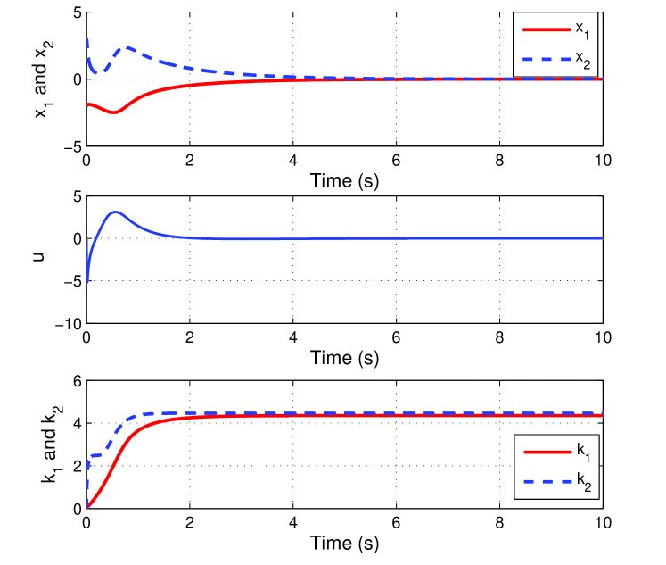
Figure 1: Simulation results for the numerical example

4.2 Realistic Example

Consider the roll control of axially symmetric Skid-To-Turn (STT) missiles, for which the simplified mathematical model with actuator dynamics is given by

$$\left\{\begin{array}[]{l}\dot{\gamma}=\omega_{x}\\ \dot{\omega}_{x}=\frac{M_{x}}{J_{x}}\\ \dot{\delta}_{x}=\frac{\delta_{xc}-\delta_{x}}{\tau_{a}}\end{array}\right.$$ (31)

where $\gamma$, $\omega_{x}$, $\delta_{x}$ and $\delta_{xc}$ are the roll angle, the rotating rate along the roll axis, the aileron deflection angle and the aileron deflection angle command to be determined, respectively. $J_{x}$, $\tau_{a}$ and $M_{x}$ are the moment of inertia about the roll axis, the time constant of the actuator and the roll moment, respectively. The mathematical expression of $M_{x}$ is given by $M_{x}=\frac{1}{2}\rho V^{2}slm_{x}$, where $\rho$, $s$, $l$ and $m_{x}$ are the air density, the reference area, the reference length, and the roll moment coefficient. Roughly speaking, $m_{x}$ can be viewed as a smooth nonlinear function of $\alpha$ (angle of attack), $\beta$ (angle of sideslip) and $\delta_{x}$ at some operating point (Please see Siouris (2004) and Hou, Liang, and Duan (2013)). When designing the roll controller for STT missiles, a frequently used way is ignoring the impacts from the pitch and the yaw channels. As a result, $m_{x}$ can be viewed as a smooth nonlinear function of $\delta_{x}$, denoted by $m_{x}(\delta_{x})$. The nominal value of $m_{x}(\delta_{x})$ can be determined by experiments and theoretical calculation. For axially symmetric missiles, $m_{x}(0)=0$. Hence, by the Mean Value Theorem, we have

$$m_{x}(\delta_{x}) = m_{x}(\delta_{x})-m_{x}(0)$$ (32)

$$= \frac{\partial m_{x}(\lambda\delta_{x})}{\partial\delta_{x}}\delta_{x}\doteq m_{x}^{\delta_{x}}(\lambda\delta_{x})\delta_{x}$$

where $\lambda\in(0,1)$ and is $\delta_{x}$-dependent. From (31) and (32), we have

$$\left\{\begin{array}[]{l}\dot{\gamma}=\omega_{x}\\ \dot{\omega}_{x}=\frac{\rho V^{2}slm_{x}^{\delta_{x}}(\lambda\delta_{x})}{2J_{x}}\delta_{x}\\ \dot{\delta}_{x}=-\frac{1}{\tau_{a}}\delta_{x}+\frac{1}{\tau_{a}}\delta_{xc}\end{array}\right.$$ (36)

The objective is to design the aileron deflection angle command $\delta_{xc}$ near some operating point such that all the states of the closed-loop system converge to zero asymptotically.

Define

$$x_{1}=\gamma,~{}x_{2}=\omega_{x},~{}x_{3}=\delta_{x},~{}u=\delta_{xc},$$

$$\theta_{1}=\frac{\rho V^{2}sl}{2J_{x}},~{}\theta_{2}=\frac{1}{\tau_{a}},$$

$$g_{2}(\delta_{x},\theta_{1})=\theta_{1}m_{x}^{\delta_{x}}(\lambda\delta_{x}),$$

$$\varphi_{3}(\delta_{x},\theta_{2})=-\theta_{2}\delta_{x},~{}g_{3}(\theta_{2})=\theta_{2},$$

then we have

$$\left\{\begin{array}[]{l}\dot{x}_{1}=x_{2}\\ \dot{x}_{2}=g_{2}(x_{3},\theta_{1})x_{3}\\ \dot{x}_{3}=\varphi_{3}(x_{3},\theta_{2})+g_{3}(\theta_{2})u\end{array}\right.$$ (40)

Generally speaking, the function $m_{x}^{\delta_{x}}(\lambda\delta_{x})=\frac{\partial m_{x}(\lambda\delta_{x})}{\partial\delta_{x}}$ are unknown, but by experience, we can assume that

$$0<m\leq m_{x}^{\delta_{x}}(\lambda\delta_{x})\leq M\xi(\delta_{x})$$

where $m$ and $M$ are two unknown constants, and $\xi(\delta_{x})$ is a positive smooth function determined by the data obtained from experiments and theoretical calculation. Near the operation point, $\theta_{1}$ continuously varies within some interval $[\theta_{1m},\theta_{1M}]$, where $\theta_{1m}$ and $\theta_{1M}$ are two positive constants, of which the values are not necessary to be known. In practice, it is not easy to determine the exact value of the time constant of the actuator $\tau_{a}$. But we know that it satisfies $\tau_{a}<0$, that is, $\theta_{2}<0$.

According to the above analysis, it is not easy to check that Assumptions 1 and 2 are satisfied if we set $\rho_{1}=0$, $\phi_{1}=1$, $\rho_{2}=0$, $\phi_{2}=\xi$, $\rho_{3}=1$, and $\phi_{3}=1$. Therefore, we could certainly design the aileron deflection angle command by strictly complying with the procedure given in Section 3. However, we could simplify the the design procedure due to the special structure of (40).

Step 0: Define

$$z_{1}=x_{1},~{}z_{2}=x_{2}-\alpha_{1},~{}z_{3}=x_{3}-\alpha_{2}$$ (41)

where $\alpha_{i}$ are virtual control laws to be determined.

Step 1: Choose

$$\alpha_{1}=-k_{1}z_{1}$$ (42)

where $k_{1}>0$ is design parameter, then one can obtain

$$\dot{z}_{1}=-k_{1}z_{1}+z_{2}$$

Define $V_{1}=\frac{1}{2}z_{1}^{2}$, then one has

$$\dot{V}_{1}=-k_{1}z_{1}^{2}+z_{1}z_{2}\leq-\left(k_{1}-\frac{\epsilon}{4}\right)z_{1}^{2}+\frac{1}{\epsilon}z_{2}^{2}$$

where $\epsilon>0$ is a constant to be determined.

Step 2: Choose

$$\alpha_{2}=-\mu_{2}k_{2}z_{2}$$ (43)

where $k_{2}$ is the update law given by

$$\dot{k}_{2}=\gamma_{2}z_{2}^{2},k_{2}(0)=k_{20}\in\Re_{>0}$$ (44)

where $\mu_{2}\in\Re_{>0}$ and $\gamma_{2}\in\Re_{>0}$ are design parameters. Then one has

$$\dot{z}_{2}=-g_{2}\mu_{2}k_{2}z_{2}+g_{2}z_{3}-k_{1}^{2}z_{1}+k_{1}z_{2}$$

Define $V_{2}=\frac{1}{2}z_{2}^{2}$, then one has

$$\dot{V}_{2}=-g_{2}\mu_{2}k_{2}z_{2}^{2}+g_{2}z_{2}z_{3}-k_{1}^{2}z_{1}z_{2}+k_{1}z_{2}^{2}$$

$$\leq-\frac{b_{2}\mu_{2}}{\gamma_{2}}k_{2}\dot{k}_{2}+B_{2}^{2}\phi_{2}^{2}z_{3}^{2}+\frac{\epsilon}{4}z_{1}^{2}+\left(\frac{k_{1}^{4}}{\epsilon}+k_{1}+\frac{1}{4}\right)z_{2}^{2}$$

Step 3: Choose

$$u=-\mu_{3}k_{3}\psi_{3}^{2}z_{3}$$ (45)

where $k_{3}$ is the update law given by

$$\dot{k}_{3}=\gamma_{3}\psi_{3}^{2}z_{3}^{2},k_{3}(0)=k_{30}\in\Re_{>0}$$ (46)

where $\psi_{3}$ is a smooth positive function to be determined, $\mu_{3}\in\Re_{>0}$ and $\gamma_{3}\in\Re_{>0}$ are design parameters. Then one has

$$\dot{z}_{3} = -\theta_{2}(z_{3}+\alpha_{2})-\theta_{2}\mu_{3}k_{3}\psi_{3}^{2}z_{3}+\mu_{2}\dot{k}_{2}z_{2}$$

$$-g_{2}\mu_{2}^{2}k_{2}^{2}z_{2}+g_{2}\mu_{2}k_{2}z_{3}-\mu_{2}k_{1}^{2}k_{2}z_{1}+\mu_{2}k_{1}k_{2}z_{2}$$

Define $V_{3}=\frac{1}{2}z_{3}^{2}$, then one has

$$\dot{V}_{3} = \theta_{2}\mu_{2}k_{2}z_{2}z_{3}-\theta_{2}z_{3}^{2}-\theta_{2}\mu_{3}k_{3}\psi_{3}^{2}z_{3}^{2}+\mu_{2}\dot{k}_{2}z_{2}z_{3}$$

$$- g_{2}\mu_{2}^{2}k_{2}^{2}z_{2}z_{3}+g_{2}\mu_{2}k_{2}z_{3}^{2}-\mu_{2}k_{1}^{2}k_{2}z_{1}z_{3}+\mu_{2}k_{1}k_{2}z_{2}z_{3}$$

$$\leq z_{2}^{2}+\frac{\epsilon}{4}z_{1}^{2}-\theta_{2}\mu_{3}k_{3}\psi_{3}^{2}z_{3}^{2}+\left(\theta_{2}^{2}\mu_{2}^{2}k_{2}^{2}+\mu_{2}^{2}\dot{k}_{2}^{2}\right.$$

$$+ \left.B_{2}^{2}\phi_{2}^{2}\mu_{2}^{4}k_{2}^{4}+\frac{1}{4}B_{2}^{2}\phi_{2}^{2}\mu_{2}^{2}k_{2}^{2}+\frac{\mu_{2}^{2}k_{1}^{4}k_{2}^{2}}{\epsilon}+\mu_{2}^{2}k_{1}^{2}k_{2}^{2}+1\right)z_{3}^{2}$$

where $\varpi=\max\{B_{2}^{2},B_{2},1\}$.

Define $V=V_{1}+V_{2}+V_{3}$, then one has

$$\dot{V} \leq -\left(k_{1}-\frac{3\epsilon}{4}\right)z_{1}^{2}-\frac{b_{2}\mu_{2}}{\gamma_{2}}k_{2}\dot{k}_{2}+\varepsilon_{1}\dot{k}_{2}-\frac{\theta_{2}\mu_{3}}{\gamma_{3}}k_{3}\dot{k}_{3}$$

$$+\varepsilon_{2}\gamma_{3}\left(\mu_{2}^{2}k_{2}^{2}+\mu_{2}^{2}\dot{k}_{2}^{2}+\phi_{2}^{2}\mu_{2}^{4}k_{2}^{4}+\frac{1}{4}\phi_{2}^{2}\mu_{2}^{2}k_{2}^{2}\right.$$

$$+\left.\frac{\mu_{2}^{2}k_{1}^{4}k_{2}^{2}}{\epsilon}+\mu_{2}^{2}k_{1}^{2}k_{2}^{2}+\phi_{2}^{2}+1\right)z_{3}^{2}$$

where $\varepsilon_{2}=\frac{1}{\gamma_{2}}\left(\frac{k_{1}^{4}+1}{\epsilon}+k_{1}+\frac{5}{4}\right)$, $\varepsilon_{3}=\frac{1}{\gamma_{3}}\max\{B_{2}^{2},\theta_{2}^{2},1\}$. Choose $\psi_{3}=\mu_{2}k_{2}+\mu_{2}\dot{k}_{2}+\phi_{2}\mu_{2}^{2}k_{2}^{2}+\frac{1}{2}\phi_{2}\mu_{2}k_{2}+\frac{\mu_{2}k_{1}^{2}k_{2}}{\sqrt{\epsilon}}+\mu_{2}k_{1}k_{2}+\phi_{2}+1$ and $\varepsilon_{1}=\left(k_{1}-\frac{3\epsilon}{4}\right)>0$, then one has

$$\dot{V}\leq-\varepsilon_{1}z_{1}^{2}-\frac{b_{2}\mu_{2}k_{2}\dot{k}_{2}}{\gamma_{2}}+\varepsilon_{2}\dot{k}_{2}-\frac{\theta_{2}\mu_{3}k_{3}\dot{k}_{3}}{\gamma_{3}}+\varepsilon_{3}\dot{k}_{3}$$

From this, we can conclude that

$$V(t)+\varepsilon_{1}\int_{0}\nolimits^{t}z_{1}^{2}(\tau)\mathrm{d}\tau \leq -\frac{b_{2}\mu_{2}k_{2}^{2}(t)}{2\gamma_{2}}-\frac{\theta_{2}\mu_{3}k_{3}^{2}(t)}{2\gamma_{3}}$$

$$+\varepsilon_{2}k_{2}(t)+\varepsilon_{3}k_{3}(t)+C_{0}$$

This means that

$$V(t)\leq-\frac{b_{2}\mu_{2}k_{2}^{2}(t)}{2\gamma_{2}}-\frac{\theta_{2}\mu_{3}k_{3}^{2}(t)}{2\gamma_{3}}+\varepsilon_{2}k_{2}(t)+\varepsilon_{3}k_{3}(t)+C_{0}$$

and

$$\varepsilon_{1}\int_{0}\nolimits^{t}z_{1}^{2}(\tau)\mathrm{d}\tau \leq -\frac{b_{2}\mu_{2}k_{2}^{2}(t)}{2\gamma_{2}}-\frac{\theta_{2}\mu_{3}k_{3}^{2}(t)}{2\gamma_{3}}+\varepsilon_{2}k_{2}(t)$$

$$+\varepsilon_{3}k_{3}(t)+C_{0}$$

Therefore, similar to the the analysis given in Section 3.2, we can firstly use the former inequality to prove that all signals in the resulting closed-loop system are bounded on $[0,\infty)$, and $\lim_{t\rightarrow\infty}x_{i}(t)=0$, $\lim_{t\rightarrow\infty}k_{i}(t)=k_{i\infty}\in\Re_{>0}$, $i=2,3$. Then, from the latter inequality, we have that $\int_{0}\nolimits^{t}z_{1}^{2}(\tau)\mathrm{d}\tau$ is bounded on $[0,\infty)$. Since $\int_{0}\nolimits^{t}z_{1}^{2}(\tau)\mathrm{d}\tau$ is a monotonic increasing function, we have that $\lim_{t\rightarrow\infty}\int_{0}\nolimits^{t}z_{1}^{2}(\tau)\mathrm{d}\tau$. So we can further use Barbalat’s lemma to prove that $\lim_{t\rightarrow\infty}x_{1}(t)=0$.

The structure parameters of some missile (Please see Hou, Liang, and Duan (2013)) are $s=0.42$ $\mathrm{m}^{2}$, $L=0.68$ $\mathrm{m}$, $J_{x}=100$ $\mathrm{kg}\cdot\mathrm{m}^{2}$, $\tau_{a}=0.01$, and its aerodynamic parameter $m_{x}^{\delta_{x}}(\lambda\delta_{x})$ at the operating point with speed $200$ $\mathrm{m}/\mathrm{s}$ and height $5$ $\mathrm{km}$ ($\rho=0.7361$ $\mathrm{kg}/\mathrm{m}^{3}$) satisfies $m\leq m_{x}^{\delta_{x}}(\lambda\delta_{x})\leq M$, where $m$ and $M$ are two unknown postive constants. Hence, we could choose $\xi=1$. For numerical simulation, we set the initial states as $\gamma(0)=10^{\circ}$, $\omega_{x}(0)=0$ ${}^{\circ}/\mathrm{s}$, $\delta_{x}(0)=0^{\circ}$, and for $i=2,3$, $\mu_{i}=0.5$, $\gamma_{i}=k_{i0}=0.1$, $k_{1}=5$, $\epsilon=0.1$, $m_{x}^{\delta_{x}}(\lambda\delta_{x})=2.12(1+0.2\sin t)$, $V=200(1+0.1\cos 2t)$. The simulation results are given in Fig. 2. All of the state variables converge to zero asymptotically.

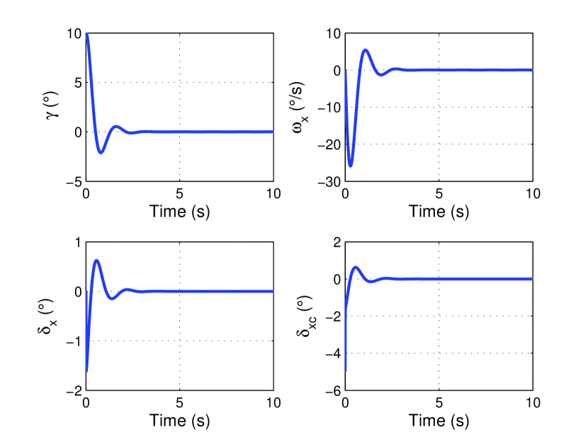
Figure 2: Simulation results for the realistic example

The simulation results of the above-mentioned numerical and realistic examples verify the correctness and the effectiveness of the proposed method.

5 Conclusion

This paper considers the globally asymptotic state stabilization problem for pure-feedback systems in the pseudo-affine form and with non-linearly parameterised uncertainties. Based on the parameter separation technique, a novel adaptive backstepping controller is designed by utilizing the high gain idea. The proposed controller could guarantee that all the closed-loop signals are bounded for any initial system condition, and that the state is globally asymptotically stabilized. A numerical and a realistic examples are given to show the correctness and effectiveness of the proposed approach.

6 Acknowledgement

This work was supported by National Natural Science Foundation of China (No.61203125,61503100), China Postdoctoral Science Foundation (No. 2014M550189), Heilongjiang Postdoctoral Fund (No. LBHZ13076) and the Fundamental Research Funds for the Central Universities (No. HIT.IBRSEM.A. 201402).

References

• Ali, Radice, and Kim (2010) Ali, I., Radice, G., and Kim, J. (2010), “Backstepping control design with actuator torque bound for spacecraft attitude maneuver”, Journal of guidance, control, and dynamics, 33(1), 254-259.
• Ferrara and Giacomini (2000) Ferrara, A., and Giacomini, L. (2000), “Control of a class of mechanical systems with uncertainties via a constructive adaptive second order VSC approach”,  Transactions of ASME, Journal of Dynamic Systems, Measurement and Control, 122(1), 33-39.
• Gao, Sun, and Liu (2012) Gao, D. X., Sun, Z. Q., and Liu, J. H. (2012), “Dynamic inversion control for a class of pure-feedback systems”, Asian Journal of Control, 14(2), 605-611.
• Gao, Sun, and Xu (2013) Gao, D., Sun, Z., and Xu, B. (2013), “Fuzzy adaptive control for pure-feedback system via time scale separation”, International Journal of Control, Automation and Systems, 11(1), 147-158.
• Hou, Duan, and Guo (2010) Hou, M. Z., Duan, G. R., and Guo M. S. (2010), “New versions of Barbalat’s lemma with applications”, Journal of Control Theory and Applications, 8(4), 545-547.
• Hou, Liang, and Duan (2013) Hou, M., Liang, X., and Duan, G. (2013), “Adaptive block dynamic surface control for integrated missile guidance and autopilot”, Chinese Journal of Aeronautics, 26(3), 741-750.
• Hunt and Mayer (1997) Hunt, L. R., and Meyer, G. (1997), “Stable inversion for nonlinear systems”, Automatica, 33(8), 1549-1554.
• Kanellakopoulos, Kokotovic, and Morse (1991) Kanellakopoulos, I., Kokotovic, P. V., and Morse, A. S. (1991), “Systematic design of adaptive controllers for feedback linearizable systems”, IEEE Transactions on Automatic Control, 36(11), 1241-1253.
• Krstic, Kanellakopoulos, and Kokotovid (1995) Krstic, M., Kanellakopoulos, I. and Kokotovid, P. V. (1995), Nonlinear and adaptive control design, New York: Wiley.
• Lei and Lin (2006) Lei, H., and Lin, W. (2006), “Universal adaptive control of nonlinear systems with unknown growth rate by output feedback”, Automatica, 42(10), 1783-1789.
• Li, Tong, and Li (2015) Li, Y., Tong, S., and Li, T. (2015) “Adaptive fuzzy backstepping control design for a class of pure-feedback switched nonlinear systems”, Nonlinear Analysis: Hybrid Systems, 16, 72-80.
• Lin and Qian (2002a) Lin, W., and Qian, C. (2002), “Adaptive control of nonlinear parameterized systems: The nonsmooth feedback framework”, IEEE Transactions on Automatic Control, 47, 757-774.
• Lin and Qian (2002b) Lin, W., and Qian, C. (2002), “Adaptive control of nonlinear parameterized systems: The smooth feedback case”, IEEE Transactions on Automatic Control, 47, 1249-1266.
• Liu (2014) Liu, Y. H. (2014), “Backstepping control for a class of pure-feedback nonlinear systems”, Control Theory $\&$ Applications, 31(6), 801-804. (in Chinese)
• Liu (2016) Liu, Y. H. (2016), “Adaptive tracking control for a class of uncertain pure-feedback systems”, International Journal of Robust and Nonlinear Control, 26(5), 1143-1154.
• Liu and Tong (2016) Liu, Y. J., and Tong, S. (2016), “Barrier Lyapunov functions-based adaptive control for a class of nonlinear pure-feedback systems with full state constraints”, Automatica, 64, 70-75.
• Lungu and Lungu (2013) Lungu, M., and Lungu, R. (2013), “Adaptive backstepping flight control for a mini-UAV”, International Journal of Adaptive Control and Signal Processing, 27(8), 635-650.
• Mnif and Yahmadi (2005) Mnif, F., and Yahmadi, A. S. (2005), “Recursive backstepping stabilization of a wheeled mobile robot”, Proceedings of the Institution of Mechanical Engineers, Part I: Journal of Systems and Control Engineering, 219(6), 419-429.
• Nijmeijer and van der (1990) Nijmeijer, H., and van der Schaft, A. (1990), Nonlinear dynamical control systems, Berlin: Springer.
• Niu, Lam, Wang, and Ho (2005) Niu, Y., Lam, J., Wang, X., and Ho, D. W. (2005), “Adaptive $H_{\infty}$ control using backstepping design and neural networks”, Journal of dynamic systems, measurement, and control, 127(3), 478-485.
• Sastry and Isidori (1989) Sastry, S. S., and Isidori, A. (1989), “Adaptive control of linearizable systems”, IEEE Transactions on Automatic Control, 34(11), 1123-1131.
• Shen, Shi, Zhang, and Lim (2014) Shen, Q., Shi, P., Zhang, T., $\&$ Lim, C. C. (2014), “Novel neural control for a class of uncertain pure-feedback systems”, IEEE Transactions on Neural Networks and Learning Systems, 25(4), 718-727.
• Siouris (2004) Siouris, G. (2004), Missile guidance and control systems. New York: Springer-Verlag.
• Slotine and Li (1991) Slotine, J. J., and Li, W. P. (1991), Applied Nonlinear Control, New Jersey: Prentice Hall.
• Sun and Liu (2007) Sun, Z., and Liu, Y. (2007), “Adaptive state-feedback stabilization for a class of high-order nonlinear uncertain systems”, Automatica, 43(10), 1772-1783.
• Sun, Wang, Li, and Peng (2013) Sun, G., Wang, D., Li, X., and Peng, Z. (2013), “A DSC approach to adaptive neural network tracking control for pure-feedback nonlinear systems”, Applied Mathematics and Computation, 219(11), 6224-6235.
• Tao (1997) Tao, G. (1997), “A simple alternative to the Barbalat lemma”, IEEE Transactions on Automatic Control, 42(5), 698.
• Wang, Hill, Ge, and Chen (2006) Wang, C., Hill, D. J., Ge, S. S., and Chen, G. (2006), “An ISS-modular approach for adaptive neural control of pure-feedback systems”, Automatica, 42(5), 723-731.
• Wang, Liu, and Shi (2011) Wang, M., Liu, X., and Shi, P. (2011), “Adaptive neural control of pure-feedback nonlinear time-delay systems via dynamic surface technique”, IEEE Transactions on Systems, Man, and Cybernetics, Part B (Cybernetics), 41(6), 1681-1692.
• Wang, Chen, and Lin (2013) Wang, H., Chen, B., and Lin, C. (2013), “Adaptive neural tracking control for a class of perturbed pure-feedback nonlinear systems”, Nonlinear Dynamics, 72(1-2), 207-220.
• Ye (1999) Ye, X. D. (1999), “Asymptotic regulation of time-varying uncertain nonlinear systems with unknown control directions”, Automatica, 35(5), 929-935.
• Yoo (2012) Yoo, S. J. (2012), “Adaptive control of non-linearly parameterised pure-feedback systems”, IET Control Theory $\&$ Applications, 6(3), 467-473.
• Yu (2013) Yu, J. (2013), “Adaptive fuzzy stabilization for a class of pure-feedback systems with unknown dead-zones”, International Journal of Fuzzy Systems, 15(3), 289-296.
• Zhang, Wen, and Zhu (2010) Zhang, T. P., Wen, H., and Zhu, Q. (2010), “Adaptive fuzzy control of nonlinear systems in pure feedback form based on input-to-state stability”, IEEE Transactions on Fuzzy Systems, 18(1), 80-93.