$l^{1}$-norm Penalized Orthogonal Forward Regression

Abstract

A $l^{1}$-norm penalized orthogonal forward regression ($l^{1}$-POFR) algorithm is proposed based on the concept of leave-one-out mean square error (LOOMSE). Firstly, a new $l^{1}$-norm penalized cost function is defined in the constructed orthogonal space, and each orthogonal basis is associated with an individually tunable regularization parameter. Secondly, due to orthogonal computation, the LOOMSE can be analytically computed without actually splitting the data set, and moreover a closed form of the optimal regularization parameter in terms of minimal LOOMSE is derived. Thirdly, a lower bound for regularization parameters is proposed, which can be used for robust LOOMSE estimation by adaptively detecting and removing regressors to an inactive set so that the computational cost of the algorithm is significantly reduced. Illustrative examples are included to demonstrate the effectiveness of this new $l^{1}$-POFR approach.

I Introduction

One of the main aims in data modeling is good generalization, i.e. the model’s capability to approximate accurately the system output for unseen data. Sparse models can be constructed using the $l^{1}$-penalized cost function, e.g. the basis pursuit or least absolute shrinkage and selection operator (LASSO) [1, 2, 3]. Based on a fixed single $l^{1}$-penalized regularization parameter, the LASSO can be configured as a standard quadratic programming optimization problem. By exploiting piecewise linearity of the problem, the least angle regression (LAR) procedure [3] is developed for solving the problem efficiently. Note that the computational efficiency in LASSO is facilitated by a single regularization parameter setting. For more complicated constraints, e.g. multiple regularizers, the cross validation by actually splitting data sets as the means of evaluating model generalization comes with considerably large overall computational overheads.

Alternatively the forward orthogonal least squares (OLS) algorithm efficiently constructs parsimonious models [4, 5]. Fundamental to the evaluation of model generalization capability is the concept of cross-validation [6], and one commonly used version of cross-validation is the leave-one-out (LOO) cross validation. For the linear-in-the-parameters models, the LOO mean square error (LOOMSE) can be calculated without actually splitting the training data set and estimating the associated models, by making use of the Sherman-Morrison-Woodbury theorem. Using the LOOMSE as the model term selective criterion to seek the model generalization, an efficient orthogonal forward regression (OFR) procedure have been introduced [7]. Furthermore, the $l^{2}$-norm based regularization techniques [8, 9, 10] have been incorporated into the OLS algorithm to produce a regularized OLS (ROLS) algorithm that carries out model term selection while reduces the variance of parameter estimate simultaneously [11]. The optimization of $l^{1}$-norm regularizer with respect to model generalization analytically is however less studied.

In this contribution, we propose a $l^{1}$-norm penalized OFR ($l^{1}$-POFR) algorithm to carry out the regularizer optimization as well as model term selection and parameter estimation simultaneously in a forward regression manner. The algorithm is based on a new $l^{1}$-norm penalized cost function with multiple $l^{1}$ regularizers, each of which is associated with an orthogonal basis vector by orthogonal decomposition of the regression matrix of the selected model terms. We derive a closed form of the optimal regularization parameter in terms of minimal LOOMSE. To save computational costs an inactive set is used along the OFR process by predicting whether any model terms will be unselectable in future regression steps.

II Preliminaries

Consider the general nonlinear system represented by the nonlinear model [13, 12]:

$$y(k)=f(\bm{x}(k))+v(k),$$ (1)

where $\bm{x}(k)=\big{[}x_{1}(k)~{}x_{2}(k)\cdots x_{m}(k)\big{]}^{\rm T}\in\mathbb{R}^{m}$ denotes the $m$-dimensional input vector at sample time index $k$ and $y(k)$ is the system output variable, respectively, while $v(k)$ denotes the system white noise and $f(\bullet)$ is the unknown system mapping.

The unknown system (1) is to be identified based on an observation data set $D_{N}=\{\bm{x}(k),y(k)\}_{k=1}^{N}$ using some suitable functional which can approximate $f(\bullet)$ with arbitrary accuracy. Without loss of generality, we use $D_{N}$ to construct a radial basis function (RBF) network model of the form

$$\widehat{y}^{(M)}(k)=f^{(M)}(\bm{x}(k))=\sum\limits_{i=1}^{M}\theta_{i}\phi_{i}(\bm{x}(k)),$$ (2)

where $\widehat{y}^{(M)}(k)$ is the model prediction output for $\bm{x}(k)$ based on the $M$-term RBF model, and $M$ is the total number of regressors or model terms, while $\theta_{i}$ are the model weights. The regressor $\phi_{i}(\bm{x})$ is given by

$$\phi_{i}(\bm{x})=\exp\Big{(}-\frac{\|\bm{x}-\bm{c}_{i}\|^{2}}{2\tau^{2}}\Big{)}$$ (3)

in which $\bm{c}_{i}=\big{[}c_{1,i}~{}c_{2,i}\cdots c_{m,i}\big{]}^{\rm T}$ is known as the center vector of the $i$th RBF unit and $\tau$ is an RBF width parameter. We assume that each RBF unit is placed on a training data, namely, all the RBF center vectors $\{\bm{c}_{i}\}_{i=1}^{M}$ are selected from the training data $\{\bm{x}(k)\}_{k=1}^{N}$, and the RBF width $\tau$ has been predetermined, for example, using cross validation.

Let us denote $e^{(M)}(k)=y(k)-\widehat{y}^{(M)}(k)$ as the $M$-term modeling error for the input data $\bm{x}(k)$. Over the training data set $D_{N}$, further denote $\bm{y}=[y(1)~{}y(2)\cdots y(N)]^{\rm T}$, $\bm{e}^{(M)}=\big{[}e^{(M)}(1)~{}e^{(M)}(2)\cdots e^{(M)}(N)\big{]}^{\rm T}$, and $\bm{\Phi}_{M}=\big{[}\bm{\phi}_{1}~{}\bm{\phi}_{2}\cdots\bm{\phi}_{M}\big{]}$ with $\bm{\phi}_{n}=\big{[}\phi_{n}(\bm{x}(1))~{}\phi_{n}(\bm{x}(2))\cdots\phi_{n}(\bm{x}(N))]^{\rm T}$, $1\leq n\leq M$. We have the $M$-term model in the matrix form of

$$\bm{y}=\bm{\Phi}_{M}\bm{\theta}_{M}+\bm{e}^{(M)},$$ (4)

where $\bm{\theta}_{M}=\big{[}\theta_{1}~{}\theta_{2}\cdots\theta_{M}\big{]}^{\rm T}$. Let an orthogonal decomposition of the regression matrix $\bm{\Phi}_{M}$ be

$$\bm{\Phi}_{M}=\bm{W}_{M}\bm{A}_{M},$$ (5)

where

$$\bm{A}_{M}=\left[\begin{array}[]{cccc}1&a_{1,2}&\cdots&a_{1,M}\\ 0&1&\ddots&\vdots\\ \vdots&\ddots&\ddots&a_{M-1,M}\\ 0&\cdots&0&1\end{array}\right]$$ (6)

and

$$\bm{W}_{M}=\big{[}\bm{w}_{1}~{}\bm{w}_{2}\cdots\bm{w}_{M}\big{]}$$ (7)

with columns satisfying $\bm{w}_{i}^{\rm T}\bm{w}_{j}=0$, if $i\neq j$. The regression model (4) can alternatively be expressed as

$$\bm{y}=\bm{W}_{M}\bm{g}_{M}+\bm{e}^{(M)},$$ (8)

where the ‘orthogonal’ model’s weight vector $\bm{g}_{M}=\big{[}g_{1}~{}g_{2}\cdots g_{M}\big{]}^{\rm T}$ satisfies the triangular system $\bm{A}_{M}\bm{\theta}_{M}=\bm{g}_{M}$, which can be used to determine the original model parameter vector $\bm{\theta}_{M}$, given $\bm{A}_{M}$ and $\bm{g}_{M}$.

Further consider the following weighted $l^{1}$-norm penalized OLS criterion for the model (8)

$$L_{e}\big{(}\bm{\Lambda}_{M},\bm{g}_{M}\big{)}=\big{\|}\bm{y}-\bm{W}_{M}\bm{g}_{M}\big{\|}^{2}+\sum_{i=1}^{M}\lambda_{i}\big{|}g_{i}\big{|},$$ (9)

where $\bm{\Lambda}_{M}=\mbox{diag}\{\lambda_{1},\lambda_{2},\cdots,\lambda_{M}\}$, which contains the local regularization parameters $\lambda_{i}\geq\varepsilon$, for $1\leq i\leq M$, and $\varepsilon>0$ is a predetermined lower bound for the regularization parameters. For a given $\bm{\Lambda}_{M}$, the solution for $\bm{g}_{M}$ can be obtained by setting the subderivative vector of $L_{e}$ to zero, i.e. ${\partial L_{e}\over\partial\bm{g}_{M}}=\bm{0}$, yielding

$$g_{i}^{({\rm olasso})}=\left(\big{|}g_{i}^{({\rm LS})}\big{|}-\frac{\lambda_{i}/2}{\bm{w}^{\rm T}_{i}\bm{w}_{i}}\right)_{+}\mbox{sign}\big{(}g_{i}^{({\rm LS})}\big{)}$$ (10)

for $1\leq i\leq M$, with the usual least squares solution given by $g_{i}^{({\rm LS)}}=\frac{\bm{w}^{\rm T}_{i}\bm{y}}{\bm{w}^{\rm T}_{i}\bm{w}_{i}}$, and the operator $(~{})_{+}$

$$z_{+}=\left\{\begin{array}[]{cc}z,&\mbox{if }z>0,\\ 0,&\mbox{if }z\leq 0.\end{array}\right.$$ (11)

Unlike the LASSO [1, 2], our objective $L_{e}\big{(}\bm{\Lambda}_{M},\bm{g}_{M}\big{)}$ is constructed on the orthogonal space and the $l^{1}$-norm parameter constraints are associated with the orthogonal bases $\bm{w}_{i}$, $1\leq i\leq M$. Since the cost function (9) contains sparsity inducing $l^{1}$ norm, some parameters $g_{i}^{({\rm olasso})}$ will be returned as zeros, producing a sparse model in the orthogonal space spanned by the columns of $\bm{W}_{M}$, which corresponds to a sparse model in the original space spanned by the columns of $\bm{\Phi}_{M}$.

III Regularization parameter optimization and model construction with LOOMSE

Each OFR stage involves the joint regularization parameter optimization, model term selection and parameter estimation. The regularization parameters with respect to their associated candidate regressors are optimized using the approximate LOOMSE formula that is derived in Section III-B, and the regressor with the smallest LOOMSE is selected.

III-A Model representation and LOOMSE in $n$-th stage OFR

Consider the OFR modeling process that has produced the $n$-term model. Let us denote the constructed $n$ columns of regressors as $\bm{W}_{n}=\big{[}\bm{w}_{1}~{}\bm{w}_{2}\cdots\bm{w}_{n}\big{]}$, with $\bm{w}_{n}=\big{[}w_{n}(1)~{}w_{n}(2)\cdots w_{n}(N)\big{]}^{\rm T}$. The model output vector of this $n$-term model is given by

$$\bm{\widehat{y}}^{(n)}=\sum_{i=1}^{n}g_{i}^{({\rm olasso})}\bm{w}_{i},$$ (12)

and the corresponding modeling error vector by $\bm{e}^{(n)}=\bm{y}-\bm{\widehat{y}}^{(n)}$. Clearly, the $n$th OFR stage can be represented by

$$\bm{e}^{(n-1)}=g_{n}\bm{w}_{n}+\bm{e}^{(n)}.$$ (13)

The model form (13) illustrates the fact that the $n$th OFR stage is simply to fit a one-variable model using the current model residual produced after the $(n-1)$th stage as the desired system output. Since $\bm{w}^{\rm T}_{n}\bm{{\hat{y}}}^{(n-1)}=0$, it is easy to verify that $g_{n}^{({\rm LS})}=\frac{\bm{w}^{\rm T}_{n}\bm{y}}{\bm{w}^{\rm T}_{n}\bm{w}_{n}}=\frac{\bm{w}^{\rm T}_{n}\bm{e}^{(n-1)}}{\bm{w}^{\rm T}_{n}\bm{w}_{n}}$.

The selection of one regressor from the candidate regressors involves initially generating candidate $\bm{w}_{n}$ by making each candidate regressor to be orthogonal to the $(n-1)$ orthogonal basis vectors, $\bm{w}_{i}$ for $1\leq i\leq n-1$ obtained in the previous $(n-1)$ OFR stages, followed by evaluating their contributions. Consider the case of $2\big{|}\bm{w}_{n}^{\rm T}\bm{e}^{(n-1)}\big{|}>\varepsilon$. Applying (10) to (13), we note that clearly as $\lambda_{n}$ decreases away from $2\big{|}\bm{w}_{n}^{\rm T}\bm{e}^{(n-1)}\big{|}$ towards $\varepsilon$, $g_{n}^{({\rm olasso})}$ increases its magnitude at a linear rate to $\lambda_{n}$, from zero to an upper bound $\big{|}g_{n}^{({\rm B})}\big{|}$ with

$$g_{n}^{({\rm B})}=\Big{(}\big{|}g_{n}^{({\rm LS})}\big{|}-\frac{\varepsilon}{2\bm{w}_{n}^{\rm T}\bm{w}_{n}}\Big{)}_{+}\mbox{sign}\big{(}g_{n}^{({\rm LS})}\big{)}.$$ (14)

For any candidate regressor, it is vital that we evaluate its potential model generalization performance using the most suitable value of $\lambda_{n}$. The optimization of the LOOMSE with respect to $\lambda_{n}$ is detailed in Section III-B, based on the idea of the LOO cross validation outlined below.

Suppose that we sequentially set aside each data point in the estimation set $D_{N}$ in turn and estimate a model using the remaining $(N-1)$ data points. The prediction error is calculated on the data point that has not been used in estimation. That is, for $k=1,2,\cdots,N$, the models are estimated based on $D_{N}\setminus(\bm{x}(k),y(k))$, respectively, and the outputs are denoted as $\widehat{y}^{(n-1,-k)}(k,\lambda_{n})$. Then, the LOO prediction error based on the $k$th data sample is calculated as

$$e^{(n,-k)}(k,\lambda_{n})=y(k)-\widehat{y}^{(n-1,-k)}(k,\lambda_{n}).$$ (15)

The LOOMSE is defined as the average of all these prediction errors, given by $J\big{(}\lambda_{n}\big{)}=E\left[\big{(}e^{(n,-k)}(k,\lambda_{n})\big{)}^{2}\right]$. Thus the optimal regularization parameter for the $n$th stage is given by

$$\lambda_{n}^{\rm opt}=\arg\,\min_{\lambda_{n}}\Big{\{}J\big{(}\lambda_{n}\big{)}=\frac{1}{N}\sum_{k=1}^{N}\big{(}e^{(n,-k)}(k,\lambda_{n})\big{)}^{2}\Big{\}}.$$ (16)

Evaluation of $J\big{(}\lambda_{n}\big{)}$ by directly splitting the data set requires extensive computational efforts. Instead, we show in Section III-B that $J\big{(}\lambda_{n}\big{)}$ can be approximately calculated without actually sequentially splitting the estimation data set. Furthermore, we also show that the optimal value $\lambda_{n}^{\rm opt}$ can be obtained in a closed-form expression.

III-B Optimal regularization parameter estimate

We notice from (10) that $g_{n}^{({\rm olasso})}=0$ if $2\big{|}\bm{w}_{n}^{\rm T}\bm{e}^{(n-1)}\big{|}<\lambda_{n}$, and thus a sufficient condition that a given $\bm{w}_{n}$ may be excluded from the candidate pool without explicitly determining $\lambda_{n}$ is $2\big{|}\bm{w}_{n}^{\rm T}\bm{e}^{(n-1)}\big{|}<\varepsilon$, which is the regularizer’s lower bound, a preset value indicating the correlation of the candidate regressor. Hence, in the following we assume that $2\big{|}\bm{w}_{n}^{\rm T}\bm{e}^{(n-1)}\big{|}>\varepsilon$, and we have

$$\bm{g}_{n}^{({\rm olasso})}=\bm{H}_{n}^{-1}\left(\bm{W}_{n}^{\rm T}\bm{y}-\bm{\Lambda}_{n}\mbox{sign}(\bm{g}_{n}^{({\rm LS})})/2\right),$$ (17)

where $\bm{g}_{n}^{({\rm olasso})}=\big{[}g_{1}^{({\rm olasso})}~{}g_{2}^{({\rm olasso})}\cdots g_{n}^{({\rm olasso})}\big{]}^{\rm T}$, $\mbox{sign}(\bm{g}_{n})$ $=\big{[}\mbox{sign}(g_{1})~{}\mbox{sign}(g_{2})\cdots\mbox{sign}(g_{n})\big{]}^{\rm T}$, and $\bm{H}_{n}=\bm{W}_{n}^{{\rm T}}\bm{W}_{n}$. Note that (17) is consistent to (10) for all terms with nonzero $g_{i}$. In the OFR procedure, any candidate terms $\bm{w}_{i}$ producing zero $g_{i}^{({\rm olasso})}$ will not be selected since they will not contribute to any reduction in the LOOMSE.

The model residual is defined by

$$e^{(n)}(k,\lambda_{n})=y(k)-\big{(}\bm{g}^{({\rm olasso})}\big{)}^{\rm T}\bm{w}(k)$$

$$=y(k)-\Big{(}\bm{y}^{\rm T}\bm{W}_{n}-\big{(}\mbox{sign}\big{(}\bm{g}^{({\rm LS})}\big{)}\big{)}^{\rm T}\bm{\Lambda}_{n}/2\Big{)}\bm{H}_{n}^{-1}\bm{w}(k),$$ (18)

where $\bm{w}(k)$ denotes the transpose of the $k$th row of $\bm{W}_{n}$. If the data sample indexed at $k$ is removed from the estimation data set, the LOO parameter estimator obtained by using only the $(N-1)$ remaining data points is given by

$$\bm{g}_{n}^{({\rm olasso},-k)}= \big{(}\bm{H}_{n}^{(-k)}\big{)}^{-1}\Big{(}\big{(}\bm{W}_{n}^{(-k)}\big{)}^{\rm T}\bm{y}^{(-k)}-$$

$$\bm{\Lambda}_{n}\mbox{sign}\big{(}\bm{g}^{({\rm LS},-k)}\big{)}/2\Big{)}$$ (19)

in which $\bm{H}_{n}^{(-k)}=\big{(}\bm{W}_{n}^{(-k)}\big{)}^{\rm T}\bm{W}^{(-k)}_{n}$, $\bm{W}_{n}^{(-k)}$ and $\bm{y}^{(-k)}$ denote the resultant regression matrix and desired output vector, respectively. It follows that we have

$$\bm{H}_{n}^{(-k)}=\bm{H}_{n}-\bm{w}(k)\bm{w}^{\rm T}(k),$$ (20)

$$\big{(}\bm{y}^{(-k)}\big{)}^{\rm T}\bm{W}_{n}^{(-k)}=\bm{y}^{\rm T}\bm{W}_{n}-y(k)\bm{w}^{\rm T}(k).$$ (21)

The LOO error evaluated at $k$ is given by

$$e^{(n,-k)}(k,\lambda_{n}) =y(k)-\big{(}\bm{g}^{({\rm olasso},-k)}\big{)}^{\rm T}\bm{w}(k)$$

$$=y(k)-\Big{(}\big{(}\bm{y}^{(-k)}\big{)}^{\rm T}\bm{W}_{n}^{(-k)}-$$

$$\big{(}\mbox{sign}\big{(}\bm{g}^{({\rm LS},-k)}\big{)}\big{)}^{\rm T}\bm{\Lambda}_{n}/2\Big{)}\big{(}\bm{H}_{n}^{(-k)}\big{)}^{-1}\bm{w}(k).$$ (22)

Applying the matrix inversion lemma to (20) yields

$$\big{(}\bm{H}_{n}^{(-k)}\big{)}^{-1}= \big{(}\bm{H}_{n}-\bm{w}(k)\bm{w}^{\rm T}(k)\big{)}^{-1}$$

$$= \bm{H}_{n}^{-1}+\frac{\bm{H}_{n}^{-1}\bm{w}(k)\bm{w}^{\rm T}(k)\bm{H}_{n}^{-1}}{1-\bm{w}^{\rm T}(k)\bm{H}_{n}^{-1}\bm{w}(k)}$$ (23)

and

$$\big{(}\bm{H}_{n}^{(-k)}\big{)}^{-1}\bm{w}(k)=\frac{\bm{H}_{n}^{-1}\bm{w}(k)}{1-\bm{w}^{\rm T}(k)\bm{H}_{n}^{-1}\bm{w}(k)}.$$ (24)

Substituting (21) and (24) into (III-B) yields

$$e^{(n,-k)}(k,\lambda_{n})=y(k)-\Big{(}\bm{y}^{\rm T}\bm{W}_{n}-y(k)\bm{w}^{\rm T}(k)-$$

$$\hskip 28.45274pt\big{(}\mbox{sign}\big{(}\bm{g}^{({\rm LS},-k)}\big{)}\big{)}^{\rm T}\bm{\Lambda}_{n}/2\Big{)}\frac{\bm{H}_{n}^{-1}\bm{w}(k)}{1-\bm{w}^{\rm T}(k)\bm{H}_{n}^{-1}\bm{w}(k)}$$

$$=\frac{y(k)-\Big{(}\bm{y}^{\rm T}\bm{W}_{n}-\big{(}\mbox{sign}\big{(}\bm{g}^{{\rm LS},-k)}\big{)}\big{)}^{\rm T}\bm{\Lambda}_{n}/2\Big{)}\bm{H}_{n}^{-1}\bm{w}(k)}{1-\bm{w}^{\rm T}(k)\bm{H}_{n}^{-1}\bm{w}(k)}.$$ (25)

Assuming that $\mbox{sign}\big{(}\bm{g}_{n}^{({\rm LS},-k)}\big{)}=\mbox{sign}\big{(}\bm{g}_{n}^{({\rm LS})}\big{)}$ holds for most data samples and then applying (III-B) to (III-B), we have

$$e^{(n,-k)}(k,\lambda_{n})=\gamma_{n}(k)e^{(n)}(k,\lambda_{n}),$$ (26)

where $\gamma_{n}(k)=\frac{1}{1-\sum_{i=1}^{n}\big{(}w_{i}(k)\big{)}^{2}\big{/}\bm{w}_{i}^{\rm T}\bm{w}_{i}}>0$, and $w_{i}(k)$ is the $k$th element of $\bm{w}_{i}$. The LOOMSE can then be calculated as

$$J\big{(}\lambda_{n}\big{)}= \frac{1}{N}\sum_{k=1}^{N}\gamma_{n}^{2}(k)\big{(}e^{(n)}(k,\lambda_{n})\big{)}^{2}.$$ (27)

We point out that in order for $\mbox{sign}\big{(}\bm{g}_{n}^{({\rm LS},-k)}\big{)}$ and $\mbox{sign}\big{(}\bm{g}_{n}^{({\rm LS})}\big{)}$ to be different, each element in $\bm{g}_{n}^{({\rm LS})}$ needs to be very close to zero, which is unlikely since only the model terms satisfying $\big{|}\bm{w}_{n}^{\rm T}\bm{e}^{(n-1)}\big{|}>\varepsilon/2$ are considered. Hence we can treat $J\big{(}\lambda_{n}\big{)}$ given in (27) as the exact LOOMSE for any preset $\varepsilon$ that is not too small.

We further represent (III-B) as

$$e^{(n)}(k,\lambda_{n})=\eta(k)+\frac{\lambda_{n}}{2\bm{w}_{n}^{\rm T}\bm{w}_{n}}w_{n}(k)\mbox{sign}\big{(}g_{n}^{({\rm LS})}\big{)},$$ (28)

where $\eta(k)=e^{(n-1)}(k)-g_{n}^{({\rm LS})}w_{n}(k)$ is the model residual obtained based on the least square estimate at the $n$th step stage. By setting ${\partial J(\lambda_{n})\over\partial\lambda_{n}}=0$, we obtain $\lambda_{n}$ in the form of the weighted least square estimate

$$\lambda_{n}=-2\mbox{sign}\big{(}g_{n}^{({\rm LS})}\big{)}\bm{w}_{n}^{\rm T}\bm{w}_{n}\bm{w}_{n}^{\rm T}\bm{\Gamma}^{(n)}\bm{\eta}\big{/}\bm{w}_{n}^{\rm T}\bm{\Gamma}^{(n)}\bm{w}_{n},$$ (29)

where $\bm{\Gamma}^{(n)}=\mbox{diag}\big{\{}\gamma_{n}^{2}(1),\gamma_{n}^{2}(2),\cdots,\gamma_{n}^{2}(N)\big{\}}$ and $\bm{\eta}=\big{[}\eta(1)~{}\eta(2)\cdots\eta(N)\big{]}^{\rm T}\in\mathbb{R}^{N}$. Finally we calculate

$$\lambda_{n}^{\rm opt}= \max\Big{\{}\min\Big{\{}2\big{|}\bm{w}_{n}^{\rm T}\bm{e}^{(n-1)}\big{|},-2\mbox{sign}\big{(}g_{n}^{({\rm LS})}\big{)}\bm{w}_{n}^{\rm T}\bm{w}_{n}$$

$$\times\bm{w}_{n}^{\rm T}\bm{\Gamma}^{(n)}\bm{\eta}\big{/}\bm{w}_{n}^{\rm T}\bm{\Gamma}^{(n)}\bm{w}_{n}\Big{\}},\varepsilon\Big{\}},$$ (30)

in order to satisfy the constraint that $\varepsilon\leq\lambda_{n}^{\rm opt}\leq 2\big{|}\bm{w}_{n}^{\rm T}\bm{e}^{(n-1)}\big{|}$. For $\lambda_{n}^{\rm opt}$ obtained using (III-B), we consider the following two cases:

1. If $\lambda_{n}^{\rm opt}=2\big{|}\bm{w}_{n}^{\rm T}\bm{e}^{(n-1)}\big{|}$, then $g_{n}^{({\rm olasso})}=0$, and this candidate regressor will not be selected.

2. If $\varepsilon\leq\lambda_{n}^{\rm opt}<2\big{|}\bm{w}_{n}^{\rm T}\bm{e}^{(n-1)}\big{|}$, then calculate $J\big{(}\lambda_{n}^{\rm opt}\big{)}$ based on $(\ref{eq:27})$ as the LOOMSE for this candidate regressor.

III-C Moving unselectable regressors to the inactive set

From Section III-B we noted that a candidate regressor satisfying $2\big{|}\bm{w}_{n}^{\rm T}\bm{e}^{(n-1)}\big{|}<\varepsilon$ does not need to be considered at the $n$th stage of selection. To save computational cost, we define the inactive set ${\mathcal{S}}$ as the index set of the unselectable regressors removed from the pool of candidates.

In the $n$th OFR stage, all the candidate regressors in the candidate pool are made orthogonal to the previously selected $(n-1)$ regressors, and the candidate with the smallest LOOMSE value is selected as the $n$th model term $\bm{w}_{n}$. Denote any other candidate regressor as $\bm{w}^{(-)}$.

Main Results: If $\big{\|}\bm{w}^{(-)}\big{\|}\cdot\big{\|}\bm{e}^{(n-1)}\big{\|}<\frac{\varepsilon}{2}$, then this candidate regressor will never be selected in further regression stages, and hence it can be moved to ${\mathcal{S}}$.

Proof: At the $(n+1)$th OFR stage, consider making the regressor $\bm{w}^{(-)}$ orthogonal to $\bm{w}_{n}$, and define

$$\bm{w}^{(+)}=\bm{w}^{(-)}-\frac{\bm{w}_{n}^{\rm T}\bm{w}^{(-)}}{\bm{w}_{n}^{\rm T}\bm{w}_{n}}\bm{w}_{n}.$$ (31)

Clearly,

$$\big{\|}\bm{w}^{(+)}\big{\|}^{2}= \Big{(}\bm{w}^{(-)}-\frac{\bm{w}_{n}^{\rm T}\bm{w}^{(-)}}{\bm{w}_{n}^{\rm T}\bm{w}_{n}}\bm{w}_{n}\Big{)}^{\rm T}\Big{(}\bm{w}^{(-)}-\frac{\bm{w}_{n}^{\rm T}\bm{w}^{(-)}}{\bm{w}_{n}^{\rm T}\bm{w}_{n}}\bm{w}_{n}\Big{)}$$

$$= \big{\|}\bm{w}^{(-)}\big{\|}^{2}-\frac{\big{(}\bm{w}_{n}^{\rm T}\bm{w}^{(-)}\big{)}^{2}}{\bm{w}_{n}^{\rm T}\bm{w}_{n}}\leq\big{\|}\bm{w}^{(-)}\big{\|}^{2}.$$ (32)

The model residual vector after the selection of $\bm{w}_{n}$ is

$$\bm{e}^{(n)}=\bm{e}^{(n-1)}-g_{n}^{({\rm olasso})}\bm{w}_{n},$$ (33)

where $g_{n}^{({\rm olasso})}$ can be written as

$$g_{n}^{({\rm olasso})}=\Big{(}\bm{w}_{n}^{\rm T}\bm{e}^{(n-1)}-\frac{\lambda_{n}}{2}\mbox{sign}\big{(}g_{n}^{({\rm LS})}\big{)}\Big{)}\big{/}\bm{w}_{n}^{\rm T}\bm{w}_{n}.$$ (34)

Thus we have

$$\big{\|}\bm{e}^{(n)}\big{\|}^{2}= \big{\|}\bm{e}^{(n-1)}\big{\|}^{2}-2g_{n}^{({\rm olasso})}\bm{w}_{n}^{\rm T}\bm{e}^{(n-1)}$$

$$+\big{(}g_{n}^{({\rm olasso})}\big{)}^{2}\bm{w}_{n}^{\rm T}\bm{w}_{n},$$ (35)

$$\big{(}g_{n}^{({\rm olasso})}\big{)}^{2}\bm{w}_{n}^{\rm T}\bm{w}_{n}= \Big{(}\big{(}\bm{w}_{n}^{\rm T}\bm{e}^{(n-1)}\big{)}^{2}-$$

$$\lambda_{n}\mbox{sign}\big{(}g_{n}^{{\rm LS})}\big{)}\bm{w}_{n}^{\rm T}\bm{e}^{(n-1)}+\frac{\lambda_{n}^{2}}{4}\Big{)}\big{/}\bm{w}_{n}^{\rm T}\bm{w}_{n},$$ (36)

and

$$2g_{n}^{({\rm olasso})}\bm{w}_{n}^{\rm T}\bm{e}^{(n-1)}= \Big{(}2\big{(}\bm{w}_{n}^{\rm T}\bm{e}^{(n-1)}\big{)}^{2}-$$

$$\lambda_{n}\mbox{sign}\big{(}g_{n}^{({\rm LS})}\big{)}\bm{w}_{n}^{\rm T}\bm{e}^{(n-1)}\Big{)}\big{/}\bm{w}_{n}^{\rm T}\bm{w}_{n}.$$ (37)

Substituting (III-C) and (III-C) into (III-C) yields

$$\big{\|}\bm{e}^{(n)}\big{\|}^{2}= \big{\|}\bm{e}^{(n-1)}\big{\|}^{2}-\Big{(}\big{(}\bm{w}_{n}^{\rm T}\bm{e}^{(n-1)}\big{)}^{2}-\frac{\lambda_{n}^{2}}{4}\Big{)}\big{/}\bm{w}_{n}^{\rm T}\bm{w}_{n}$$

$$< \big{\|}\bm{e}^{(n-1)}\big{\|}^{2},$$ (38)

due to the fact that $\big{|}\bm{w}_{n}^{\rm T}\bm{e}^{(n-1)}\big{|}>\frac{\lambda_{n}}{2}$. From (III-C) and (III-C), it can be concluded that

$$\big{\|}\bm{w}^{(+)}\big{\|}\cdot\big{\|}\bm{e}^{(n)}\big{\|}<\big{\|}\bm{w}^{(-)}\big{\|}\cdot\big{\|}\bm{e}^{(n-1)}\big{\|}<\frac{\varepsilon}{2}.$$ (39)

Since $\big{\|}\bm{w}^{(+)}\big{\|}\cdot\big{\|}\bm{e}^{(n)}\big{\|}$ is the upper bound of $\Big{|}\big{(}\bm{w}^{(+)}\big{)}^{\rm T}\bm{e}^{(n)}\Big{|}$, this means that this regressor will not be selected at the $(n+1)$th stage. By induction, it will never be selected in further regression stages, and hence it can be moved to ${\mathcal{S}}$.

IV The proposed $l^{1}$-POFR algorithm

The proposed $l^{1}$-POFR algorithm integrates (i) the model regressor selection based on minimizing the LOOMSE; (ii) regularization parameter optimization also based on minimizing the LOOMSE; and (iii) the mechanism of removing unproductive candidate regressors during the OFR procedure. Define

$$\bm{\Phi}^{(n-1)}=\big{[}\bm{w}_{1}\cdots\bm{w}_{n-1}~{}\bm{\phi}_{n}^{(n-1)}\cdots\bm{\phi}_{M}^{(n-1)}\big{]}\in\mathbb{R}^{N\times M},$$ (40)

with $\bm{\Phi}^{(0)}=\bm{\Phi}_{M}$. If some of the columns in $\bm{\Phi}^{(n-1)}$ have been interchanged, this will still be referred as $\bm{\Phi}^{(n-1)}$ for notational simplicity.

TABLE I: The $n$th stage of the selection procedure.

For $\{n\leq j\leq M\}\cap\{j\notin{\mathcal{S}}\}$, denote the $k$th element of $\bm{\phi}_{j}^{(n-1)}$ as $\phi_{j}^{(n-1)}(k)$ and compute $\alpha_{j}=\big{(}\bm{\phi}_{j}^{(n-1)}\big{)}^{\rm T}\bm{e}^{(n-1)}$, and $\beta_{j}=\big{\|}\bm{\phi}_{j}^{(n-1)}\big{\|}\cdot\big{\|}\bm{e}^{(n-1)}\big{\|}$. Step 1): If $\beta_{j}<\varepsilon/2$, ${\mathcal{S}}={\mathcal{S}}\cup j$; Else if $\big{|}\alpha_{j}\big{|}<\varepsilon/2$, set $J_{n}^{(j)}$ as a very large positive number so that it will not be selected in Step 4). Otherwise goto step 2). Step 2): Calculate $\displaystyle\kappa_{n}^{(j)}$ $\displaystyle=$ $\displaystyle\big{(}\bm{\phi}_{j}^{(n-1)}\big{)}^{\rm T}\bm{\phi}_{j}^{(n-1)},$ (41) $\displaystyle g_{n}^{({\rm LS},j)}$ $\displaystyle=$ $\displaystyle\frac{\alpha_{j}}{\kappa_{n}^{(j)}},$ (42) $\displaystyle\bm{\Gamma}^{(n,j)}$ $\displaystyle=$ $\displaystyle\mbox{diag}\left\{\frac{1}{\Big{(}\zeta^{(n-1)}(1)-\big{(}\phi_{j}^{(n-1)}(1)\big{)}^{2}\big{/}\kappa_{n}^{(j)}\Big{)}^{2}},\right.$ (43) $\displaystyle\frac{1}{\Big{(}\zeta^{(n-1)}(2)-\big{(}\phi_{j}^{(n-1)}(2)\big{)}^{2}\big{/}\kappa_{n}^{(j)}\Big{)}^{2}},\cdots,$ $\displaystyle\left.\frac{1}{\Big{(}\zeta^{(n-1)}(N)-\big{(}\phi_{j}^{(n-1)}(N)\big{)}^{2}\big{/}\kappa_{n}^{(j)}\Big{)}^{2}}\right\}\in\mathbb{R}^{N\times N},$ $\displaystyle\bm{\eta}^{(j)}$ $\displaystyle=$ $\displaystyle\bm{e}^{(n-1)}-g_{n}^{({\rm LS},j)}\bm{\phi}_{j}^{(n-1)},$ (44) $\displaystyle\lambda_{n}^{({\rm opt},j)}$ $\displaystyle=$ $\displaystyle\max\Big{\{}\min\Big{\{}2\big{|}\alpha_{j}\big{|},-2\mbox{sign}\big{(}g_{n}^{({\rm LS},j)}\big{)}\kappa_{n}^{(j)}$ (45) $\displaystyle\big{(}\bm{\phi}_{j}^{(n-1)}\big{)}^{\rm T}\bm{\Gamma}^{(n,j)}\bm{\eta}^{(j)}\big{/}\big{(}\bm{\phi}_{j}^{(n-1)}\big{)}^{\rm T}\bm{\Gamma}^{(n,j)}\bm{\phi}_{j}^{(n-1)}\Big{\}},\varepsilon\Big{\}}.$ Step 3): If $\lambda_{n}^{({\rm opt},j)}=2\big{|}\alpha_{j}\big{|}$, set $J_{n}^{(j)}$ as a very large positive number so that it will not be selected in Step 4); Otherwise calculate $\displaystyle g_{n}^{({\rm olasso},j)}$ $\displaystyle=$ $\displaystyle\big{(}\big{|}g_{n}^{({\rm LS},j)}\big{|}-\frac{\lambda_{n}^{({\rm opt},j)}/2}{\kappa_{n}^{(j)}}\big{)}_{+}\mbox{sign}\big{(}g_{n}^{({\rm LS},j)}\big{)},$ (46) $\displaystyle\bm{e}^{(n,j)}$ $\displaystyle=$ $\displaystyle\bm{e}^{(n-1)}-g_{n}^{({\rm olasso},j)}\bm{\phi}_{j}^{(n-1)},$ (47) $\displaystyle J_{n}^{(j)}$ $\displaystyle=$ $\displaystyle\big{(}\bm{e}^{(n,j)}\big{)}^{\rm T}\bm{\Gamma}^{(n,j)}\bm{e}^{(n,j)}/N.$ (48) Step 4): Find $$J_{n}=J_{n}^{(j_{n})}=\min\left\{J_{n}^{(j)},\ \{l\leq j\leq M\}\cap\{j\notin{\mathcal{S}}\}\right\}.$$ (49) Then update $\bm{e}^{(n)}$ and $g_{n}^{({\rm olasso})}$ as $\bm{e}^{(n,j_{n})}$ and $g_{n}^{({\rm olasso},j_{n})}$, respectively. The $j_{n}$th and the $n$th columns of $\bm{\Phi}^{(n-1)}$ are interchanged, while the $j_{n}$th column and the $n$th column of $\bm{A}_{M}$ are interchanged up to the $(n-1)$th row. This effectively selects the $n$th regressor in the subset model. The modified Gram-Schmidt orthogonalisation procedure [4] then calculates the $n$th row of the matrix $\bm{A}_{M}$ and transfers $\bm{\Phi}^{(n-1)}$ into $\bm{\Phi}^{(n)}$ as follows $$\!\!\!\left.\!\!\!\begin{array}[]{l}\bm{w}_{n}=\bm{\phi}_{n}^{(n-1)},\\ a_{n,j}=\bm{w}_{n}^{\rm T}\bm{\phi}_{j}^{(n-1)}\big{/}\bm{w}_{n}^{\rm T}\bm{w}_{n},\{n+1\leq j\leq M\}\cap\{j\notin{\mathcal{S}}\},\\ \bm{\phi}_{j}^{(n)}=\bm{\phi}_{j}^{(n-1)}-a_{n,j}\bm{w}_{n},\{n+1\leq j\leq M\}\cap\{j\notin{\mathcal{S}}\}.\end{array}\!\!\!\right\}\!\!\!$$ (50) Then update $\zeta^{(n)}(k)=\zeta^{(n-1)}(k)-\big{(}w_{n}(k)\big{)}^{2}\big{/}\bm{w}_{n}^{\rm T}\bm{w}_{n}$ for $1\leq k\leq N$.

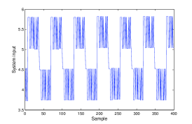
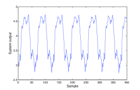
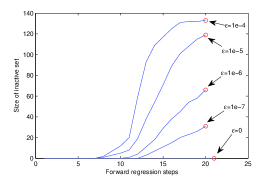
(a)                                                (b)                                                (c)

Figure 1: Engine Data: (a) the system input $u(k)$, (b) the system output $y(k)$, and (c) the evolution of the size of ${\mathcal{S}}$ with respect to the chosen $\varepsilon$.

The initial conditions are as follows. Preset $\varepsilon>0$ as a very small value. Set $\bm{e}^{(0)}=\bm{y}$, $\zeta^{(0)}(k)=1$ for $1\leq k\leq N$, and ${\mathcal{S}}$ as the empty set $\emptyset$. The $n$th stage of the selection procedure is listed in Table I. The OFR procedure is automatically terminated at the $(n_{s}+1)$th stage when the condition

$$J_{n_{s}+1}\geq J_{n_{s}}$$ (51)

is detected, yielding a subset model with $n_{s}$ significant regressors. It is worth emphasizing that there always exists a model size $n_{s}$, and for $n\leq n_{s}$, the LOOMSE $J_{n}$ decreases as $n$ increases, while the condition (51) holds [7, 14].

Note that the LOOMSE is used not only for deriving the closed form of the optimal regularization parameter estimate $\lambda_{n}^{\rm opt}$ but also for selecting the most significant model regressor. Specifically, a regressor is selected as the one that produces the smallest LOOMSE value as well as offering the reduction in the LOOMSE. After the $n_{s}$ stage when there is no reduction in the LOOMSE criterion for a few consecutive OFR stages, the model construction procedure can be terminated. Thus, the $l^{1}$-POFR algorithm automatically constructs a sparse $n_{s}$-term model, where typically $n_{s}\ll M$.

Also note that it is assumed that $\varepsilon$ should not be too small such that the LOOMSE estimation formula can be considered to be accurate. This means that if $\varepsilon$ is set too low, many insignificant candidate regressors will have inaccurate LOOMSE values for competition. However, we emphasize that these terms with inaccurate LOOMSE values will not be selected as the winner to enter the model. Hence in practice we only need to make sure that $\varepsilon$ is not too large, which would introduce unnecessary bias to the model parameter estimates. Clearly, a relatively larger $\varepsilon$ will save computational costs by 1) resulting in a sparser model, and 2) producing a larger sized inactive set during the OFR process.

Finally, regarding the computational complexity of the $l^{1}$-POFR algorithm, if the unproductive regressors are not removed to the inactive set ${\mathcal{S}}$ during the OFR procedure, it is well known that the computational cost is in the order of $\textsf{O}(N)$ for evaluating each candidate regressor [14]. The total computational cost then needs to be scaled by the number of evaluations in forward regression, which is $M(M-n_{s})/2$. By removing unproductive regressors to ${\mathcal{S}}$ during the OFR procedure, the computational cost can obviously be reduced significantly. It is not possible to exactly assess the computational cost saving due to removing the unproductive regressors, as this is problem dependent.

TABLE II: Comparison of the modeling performance for Engine Data. The computational cost saving is based on the same size of model without removing unproductive regressors in the $l^{1}$-POFR.

Algorithm	MSE	MSE	Model	Cost
	training set	test set	size	saving
LROLS-LOO [14]	$0.000453$	$0.000490$	$22$	NA
$\varepsilon$-SVM ($\tau=3$)	$0.000502$	$0.000482$	$208$	NA
$\varepsilon$-SVM ($\tau=2.5$)	$0.000480$	$0.000475$	$208$	NA
$\varepsilon$-SVM ($\tau=2$)	$0.000461$	$0.000486$	$208$	NA
$\varepsilon$-SVM ($\tau=1.5$)	$0.000415$	$0.000579$	$208$	NA
$\varepsilon$-SVM ($\tau=1$)	$0.000370$	$0.000794$	$208$	NA
LASSO ($\tau=1.5$)	$0.000923$	$0.001010$	$70$	NA
LASSO ($\tau=1$)	$0.000708$	$0.000748$	$44$	NA
LASSO ($\tau=0.5$)	$0.000706$	$0.000842$	$54$	NA
LASSO ($\tau=0.2$)	$0.000565$	$0.000800$	$81$	NA
LASSO ($\tau=0.1$)	$0.000644$	$0.001907$	$76$	NA
$l^{1}$-POFR ($\varepsilon=10^{-4}$)	$0.000498$	$0.000502$	$20$	27%
$l^{1}$-POFR ($\varepsilon=10^{-5}$)	$0.000492$	$0.000480$	$20$	18%
$l^{1}$-POFR ($\varepsilon=10^{-6}$)	$0.000484$	$0.000485$	$20$	8%
$l^{1}$-POFR ($\varepsilon=10^{-7}$)	$0.000481$	$0.000476$	$20$	3%
$l^{1}$-POFR ($\varepsilon=0$)	$0.000452$	$0.000472$	$21$	0%

V Simulation Study

Example 1: This Engine Data set [15] contains the 410 data samples of the fuel rack position (the input $u(k)$) and the engine speed (the output $y(k)$), collected from a Leyland TL11 turbocharged, direct injection diesel engine which was operated at a low engine speed. The 410 input and output data points of the engine data set are plotted in Fig. 1 (a) and (b), respectively. The first $210$ data samples were used in training and the last $200$ data samples for model testing. The previous study has shown that the data set can be modeled adequately using the system input vector $\bm{x}(k)=\big{[}y(k-1)~{}u(k-1)~{}u(k-2)]^{\rm T}$, and the best Gaussian RBF model was provided by the $l^{2}$-norm local regularization assisted OLS (LROLS) algorithm based on the LOOMSE (LROLS-LOO) [14] which was quoted in Table II for comparison. The $\varepsilon$-SVM algorithm [16] and the LASSO were also experimented based on the Gaussian kernel with a common variance $\tau^{2}$. For the $\varepsilon$-SVM, the Matlab function quadprog.m was used with the algorithm option set as ‘interior-point-convex’. The tuning parameters in the $\varepsilon$-SVM algorithm, such as soft margin parameter $C$ [16], were set empirically so that the best possible result was obtained after several trials. For the LASSO, the Matlab function lasso.m was used with 10-fold CV being used to select the associated regularization parameter. For both the $\varepsilon$-SVM and LASSO, we list the results obtained for a range of kernel width $\tau$ values in Table II, for comparison.

Similar to the LROLS-LOO algorithm [14], we also used the Gaussian RBF kernel (3) for the proposed $l^{1}$-POFR algorithm with an empirically set $\tau=2.5$ and the RBF centers $\bm{c}_{i}$ were formed using all the training data samples. With a preset value of $\varepsilon$, a sparse model of size $n_{s}$ was automatically selected when the condition (51) was met. Fig. 1 (c) illustrates the evolution of the size of ${\mathcal{S}}$ with respect to a range of the preset $\varepsilon$ values. The test MSE values produced by the sparse models and the sizes of the models associated with the same range of $\varepsilon$ values are recorded in Table II, which show that the excellent model generalization capability of all the models generated by the proposed algorithm. Moreover, the $l^{1}$-POFR algorithm produces the sparsest model.

TABLE III: Comparison of the modeling performance for Boston House Data. The results were averaged over 100 realizations and given as $\mbox{mean}\pm\mbox{standard deviation}$.

Algorithm	MSE	MSE	Model
	training set	test set	size
$\varepsilon$-SVM [16]	$6.80\pm 0.44$	$23.18\pm 9.05$	$243\pm 5.3$
LROLS-LOO [14]	$12.97\pm 2.67$	$17.42\pm 4.67$	$58.6\pm 11.3$
NonOFR-LOO [18]	$10.10\pm 3.40$	$14.07\pm 3.62$	$34.6\pm 8.4$
LASSO ($\tau=2$)	$8.52\pm 3.57$	$14.37\pm 8.15$	$76.8\pm 39.7$
LASSO ($\tau=3$)	$8.55\pm 1.07$	$13.31\pm 6.65$	$68.6\pm 29.3$
LASSO ($\tau=5$)	$10.45\pm 1.07$	$15.05\pm 8.37$	$85.9\pm 19.7$
LASSO ($\tau=10$)	$16.42\pm 1.78$	$19.39\pm 8.31$	$29.9\pm 21.3$
$l^{1}$-POFR ($\varepsilon=0.01$)	$9.99\pm 1.37$	$14.47\pm 7.47$	$30.5\pm 5.3$
$l^{1}$-POFR ($\varepsilon=0.001$)	$9.24\pm 1.57$	$14.10\pm 7.02$	$34.9\pm 7.8$
$l^{1}$-POFR ($\varepsilon=0.0001$)	$9.07\pm 1.64$	$14.02\pm 6.85$	$36.6\pm 9.3$
$l^{1}$-POFR ($\varepsilon=0.00001$)	$9.08\pm 1.64$	$13.95\pm 6.76$	$36.5\pm 9.3$

Example 2: This regression benchmark data set, Boston Housing Data, is available at the UCI repository [17]. The data set comprises 506 data points with 14 variables. The previous study [18] performed the task of predicting the median house value from the remaining 13 attributes using the $\varepsilon$-SVM [16], the LROLS-LOO [14] and the nonlinear OFR based on the LOOMSE (NonOFR-LOO) [18]. The NonOFR-LOO algorithm [18] constructs a nonlinear RBF model in the OFR procedure, where each stage of the OFR determines one RBF node’s center vector and diagonal covariance matrix by minimizing the LOOMSE. In the experiment study presented in [18], 456 data points were randomly selected from the data set for training and the remaining 50 data points were used to form the test set. Average results were given over 100 realizations. For each realization, 13 input attributes were normalized so that each attribute had zero mean and standard deviation of one. We also experimented with the LASSO supplied by Matlab lasso.m with option set as 10-fold CV to select the associated regularization parameter. For the LASSO, a common kernel width $\tau$ was set for constructing the kernel model from the 456 candidate regressors of each realization, and a range of $\tau$ values were experimented.

For the $l^{1}$-POFR, $\tau=15$ was empirically set for constructing 456 candidate Gaussian RBF regressors of each realization. We experimented a range of the preset $\varepsilon$ values for the $l^{1}$-POFR algorithm, and the results obtained are as summarized in Table III, in comparison with the results obtained by the $\varepsilon$-SVM and the LASSO, as well as the LROLS-LOO and NonOFR-LOO, which are quoted from the study [18].

VI Conclusions

We have developed an efficient data model algorithm, referred to as the $l^{1}$-norm penalized orthogonal forward regression ($l^{1}$-POFR), for linear-in-the-parameters nonlinear models based on a new $l^{1}$-norm penalized cost function defined in the constructed orthogonal modeling space. The LOOMSE is used for simultaneous model term selection and regularization parameter estimation in a highly efficient OFR procedure. Additionally, we have proposed a lower bound of the regularisation parameters for robust LOOMSE estimation as well as detecting and removing insignificant regressors to an inactive set along the OFR process, further enhancing the efficiency of the OFR procedure. Numerical studies have been utilized to demonstrate the effectiveness of this new $l^{1}$-POFR approach.

References

- [1] S. S. Chen, D. L. Donoho, and M. A. Saunders, “Atomic decomposition by basis pursuit,” SIAM J. Scientific Computing, vol. 20, no. 1, pp. 33–61, 1998.
- [2] R. Tibshirani, “Regression shrinkage and selection via the lasso,” J. Royal Statistical Society, Series B, vol. 58, no. 1, pp. 267–288, 1996.
- [3] B. Efron, T. Hastie, I. Johnstone, and R. Tibshirani, “Least angle regression,” Annals of Statistics, vol. 32, no. 2, pp. 407–451, 2004.
- [4] S. Chen, S. A. Billings, and W. Luo, “Orthogonal least squares methods and their applications to non-linear system identification,” Int. J. Control, vol. 50, no. 5, pp. 1873–1896, 1989.
- [5] S. Chen, C. F. N. Cowan, and P. M. Grant, “Orthogonal least squares learning algorithm for radial basis function networks,” IEEE Trans. Neural Networks, vol. 2, no. 2, pp. 302–309, Mar. 1991.
- [6] M. Stone,“Cross-validatory choice and assessment of statistical predictions,” HJ. Royal Statistical Society, Series B, vol. 36, no. 2, pp. 111–147, 1974.
- [7] X. Hong, P. M. Sharkey, and K. Warwick, “Automatic nonlinear predictive model-construction using forward regression and the PRESS statistic,” IEE Proc. Control Theory Applications, vol. 150, no. 3, pp. 245–254, 2003.
- [8] D. J. C. MacKay, Bayesian Methods for Adaptive Models. Ph.D. thesis, California Institute of Technology, USA, 1991.
- [9] S. Chen, E. S. Chng, and K. Alkadhimi, “Regularised orthogonal least squares algorithm for constructing radial basis function networks,” Int. J. Control, vol. 64, no. 5, pp. 829–837, 1996.
- [10] M. J. L. Orr, “Regularisation in the selection of radial basis function centers,” Neural Computation, vol. 7, no. 3, pp. 606–623, 1995.
- [11] S. Chen, X. Hong, and C. J. Harris, “Sparse kernel regression modelling using combined locally regularised orthogonal least squares and D-optimality experimental design,” IEEE Trans. Automatic Control, vol. 48, no. 6, pp. 1029–1036, June 2003.
- [12] S. Chen and S. A. Billings, “Representation of nonlinear systems: The NARMAX model,” Int. J. Control, vol. 49, no. 3, pp. 1013–1032, 1989.
- [13] C. J. Harris, X. Hong, and Q. Gan, Adaptive Modelling, Estimation and Fusion from Data: A Neurofuzzy Approach. Springer-Verlag, 2002.
- [14] S. Chen, X. Hong, C. J. Harris, and P. M. Sharkey, “Sparse modelling using orthogonal forward regression with PRESS statistic and regularization,” IEEE Trans. Systems, Man and Cybernetics, Part B: Cybernetics, vol. 34, no. 2, pp. 898–911, Apr. 2004.
- [15] S. A. Billings, S. Chen, and R. J. Backhouse, “The identification of linear and non-linear models of a turbocharged automotive diesel engine,” Mechanical Systems and Signal Processing, vol. 3, no. 2, pp. 123–142, 1989.
- [16] S. R. Gun, “Support vector machines for classification and regression,” Research Report, Dept. Electronics and Computer Science, University of Southampton, U.K, 1998.
- [17] A. Frank and A. Asuncion, “UCI machine learning repository,” 2010.
- [18] S. Chen, X. Hong, and C. J. Harris, “Construction of tunable radial basis function networks using orthogonal forward selection,” IEEE Trans. Trans. on Systems, Man and Cybernetics, Part B: Cybernetics, vol. 39, no. 2, pp. 457–466, Apr. 2009.