Slow Lévy flights

Abstract

Among Markovian processes, the hallmark of Lévy flights is superdiffusion, or faster-than-Brownian dynamics. Here we show that Lévy laws, as well as Gaussians, can also be the limit distributions of processes with long range memory that exhibit very slow diffusion, logarithmic in time. These processes are path-dependent and anomalous motion emerges from frequent relocations to already visited sites. We show how the Central Limit Theorem is modified in this context, keeping the usual distinction between analytic and non-analytic characteristic functions. A fluctuation-dissipation relation is also derived. Our results may have important applications in the study of animal and human displacements.

I Introduction

Lévy flights (LFs) represent one of the most important extensions of the Central Limit Theorem (CLT), a cornerstone of probability theory feller ; alpha . LFs are sums of independent and identically distributed random variables that admit non-Gaussian limit laws due to their very large fluctuations. They find physical applications in laser cooling bardou , optics light or chaotic transport strangekin . LFs are also paradigmatic of superdiffusive processes, i.e., anomalous types of transport where the characteristic diffusive length scale $l(t)$ of an individual particle grows with time as $t^{\alpha}$ with $\alpha>1/2$, that is, faster than in the classical Brownian motion (BM) bouchaud ; rainer ; klafterphysrep ; weiss .

In recent years, LFs (as well as the related Lévy walks lw ) have become prominent for modeling diffusion in a variety of complex systems. Power-law distributions of step lengths with diverging variance, a key feature of Lévy processes, are found to describe well the trajectories of immune cells in the brain tcells , the displacements of animals gandhi ; levy2 ; sims ; gab and hunter-gatherers brown ; pnas2014 in their environments, or the travels of modern humans within and between cities geisel ; rhee ; gonzalez ; song . However, the assumption of independence between steps does limit the applicability of genuine Lévy processes for modeling real systems, where non-Markovian effects and correlations can be strong. Deeper analysis of empirical data actually reveals that the diffusion of humans and animals (even those exhibiting Lévy patterns) is in general subdiffusive at large times, i.e., with $l(t)\ll t^{1/2}$ song ; gautestad2005 ; gautestad2006 ; borger ; solis . Furthermore, $l(t)$ commonly grows more slowly than a power-law of time, namely, in a logarithmic way borger ; song ; solis : this behavior is even in sharper contrast with the superdiffusion of simple LFs.

Logarithmic diffusion can be generated in several ways, for instance, by continuous time random walks models with superheavy-tailed distributions of waiting times kantz , or by certain iterated maps drager ; sokolov . In the context of animal and human mobility, an important but little explored mechanism that may lead to very slow subdiffusion is spatial memory: many living organisms actually keep revisiting familiar places fagan ; gautestad2005 ; gautestad2006 ; vanmoorter ; borger ; solis . Here, we seek to understand, with the help of a solvable model, how this type of memory can act as a self-attracting force which drastically constrains diffusion towards limited areas, giving rise to “home ranges”, and how this property can still be compatible with power-law distributed step lengths.

The dynamics and limit distributions of constrained LFs are not well understood, except for processes subjected to long waiting times or in external potentials, mainly klafterphysrep ; compet . Several limit theorems also exist for specific problems of sums of correlated random variables hilhorst , and a few random walks with infinite memory of their previous displacements have exactly solvable first moments elephant ; kumar ; dasilva . Yet, very little is known on LFs composed of non-independent steps, in particular processes with self-attraction. Self-attracting random walks are path-dependent processes where a walker tends to return to previously visited sites davis ; annals . Numerical simulations and scaling arguments clearly show that self-attracting walks can exhibit subdiffusion quasistatic ; grassberger ; siam . These mathematically challenging processes cannot be readily analyzed with better known frameworks for subdiffusive phenomena, such as fractional Fokker-Planck equations klafterphysrep or scaled Brownian motions sbm ; slowsbm . They are more related with diffusion in quenched disordered media bouchaud , where some rigorous connections have been made with the Sinai model matteo .

In this study, we heuristically modify the CLT for processes that exhibit very slow diffusion, and show that such modification exactly describes a class of self-attracting LF and self-attracting random walks. The characteristic functions having a similar structure than in the ordinary CLT, Gaussian and Lévy distributions emerge asymptotically in space, although the dynamics is strongly subdiffusive. We also derive a fluctuation-dissipation relation in the Gaussian case.

II General formulation

Let $P(n,t)$ be the probability that the position $X_{t}$ of a particle at time $t$ is $n$ (where $n$ and $t$ are discrete), given that the particle is located at the origin $n=0$ at $t=0$. We consider discrete, one dimensional walks, keeping in mind that discreteness is not relevant in the asymptotic limit. The results can also be extended higher dimensions straightforwardly.

We recall that for a standard random walk composed of $t$ i.i.d. displacements $\ell_{i}$ with distribution $p(\ell)$, the characteristic function of $X_{t}$, defined as $\widetilde{P}(k,t)\equiv\sum_{n=-\infty}^{\infty}e^{-ikn}P(n,t)=\langle e^{-ikX_{t}}\rangle$, takes the form weiss :

$$\widetilde{P}(k,t)=\tilde{p}(k)^{t}=e^{\ln[\tilde{p}(k)]t},$$ (1)

where $\tilde{p}(k)$ is the characteristic function of $\ell$. Since $\tilde{p}(0)=1$ by normalization, in the unbiased ($\langle\ell\rangle=0$) and symmetric case, an expansion near $k=0$ gives:

$$\tilde{p}(k)=1-C|k|^{\mu}+...$$ (2)

Two basic situations emerge: the analytic case $\mu=2$, corresponding to $\langle\ell^{2}\rangle<\infty$ (and $C=\langle\ell^{2}\rangle/2$), and the non-analytic case $0<\mu<2$ when $\langle\ell^{2}\rangle$ does not exist, due to a power-law decay of $p(\ell)$:

$$p(\ell)\sim 1/|\ell|^{1+\mu}$$ (3)

at large $\ell$ weiss . Combining (1)-(2) yields the celebrated Gaussian-Lévy CLT:

$$\widetilde{P}(k,t)\rightarrow e^{-C|k|^{\mu}t}.$$ (4)

Eq. (4) implies a scaling law $P(n,t)\rightarrow t^{-1/\mu}f(n/t^{1/\mu})$ where the scaling function $f(x)$ is a Gaussian or a symmetric Lévy law $L_{\mu,0}(x)$, for $\mu=2$ and $0<\mu<2$, respectively. The latter case is superdiffusive as the typical diffusion length is $\propto t^{1/\mu}\gg t^{1/2}$.

Consider now a simple modification of Eq. (1): suppose that for certain diffusion processes with memory or sums of correlated random variables (we do not need to specify a model at this point), $\widetilde{P}$ is not an exponential function of $t$ but a power-law:

$$\widetilde{P}(k,t)\simeq t^{-a(k)}=e^{-a(k)\ln t},$$ (5)

at large $t$ and small $k$. The function $a(k)$ satisfies $a(0)=0$, owing to the normalization $\widetilde{P}(k=0,t)=1$. Again, $a(k)$ can be generically analytic or non-analytic near $k=0$. In the first case, since $\widetilde{P}(k,t)^{*}=\widetilde{P}(-k,t)$ and $|\widetilde{P}(k,t)|\leq 1$, the Taylor expansion of the exponent must be of the form $a(k)\simeq ia_{1}k+a_{2}k^{2}+...$, with $a_{1}$ and $a_{2}$ two real constants and $a_{2}>0$. For simplicity, we first consider $a_{1}=0$, or motion without bias.

In the non-analytic case, the same arguments lead to $a(k)\simeq a_{\mu}|k|^{\mu}$ with $0<\mu<2$ a priori, and $a_{\mu}>0$. Inserting into (5), we see that the main difference with (4) is that the variable $t$ is substituted by $\ln t$. Hence:

$$P(n,t)\rightarrow\frac{1}{(\ln t)^{1/\mu}}\ f_{\mu}\left(\frac{n}{(\ln t)^{1/\mu}}\right),$$ (6)

where the limit laws $f_{\mu}(x)$ are the same as in the ordinary CLT. If $\mu=2$, diffusion is Gaussian but very slow: $\langle X_{t}^{2}\rangle=2a_{2}\ln t$, in sharp contrast with BM, where $\langle X_{t}^{2}\rangle=2Dt$. [In this case, Eq. (6) should not be confused with the log-normal distribution, where the logarithm applies to the space variable, not the temporal one.] A basic Markovian example is, by construction, a scaled Brownian motion, which is a BM where the time $T$ is rescaled as $t=e^{T}$. Such process is also equivalent to a BM with a time-dependent diffusion coefficient, $D(t)$, decaying as $1/t$ at large $t$ slowsbm .

In the non-analytic case, the situation looks paradoxical at first sight. The ensemble average $\langle X_{t}^{2}\rangle=\infty$ like in ordinary Lévy processes due to the broad tails of $L_{\mu,0}(x)$ (or due to the fact that $\partial^{2}P(k,t)/\partial k^{2}$ does not exist at $k=0$, from Eq.(5)). Yet, Eq. (6) also defines a typical diffusion length $l(t)\propto(\ln t)^{1/\mu}$, which grows extremely slowly. Therefore, based on this scaling length $l(t)$, motion is strongly subdiffusive and all the finite moments, $\langle|X_{t}|^{\nu}\rangle$ with $\nu<\mu$, also evolve very slowly, as $(\ln t)^{\nu/\mu}$. Still, the process keeps superdiffusive features through the divergence of the second moment. This situation is reminiscent of scaling violation, which also arises in continuous time random walks schmiedeberg or Lévy walks lw ; fleurov .

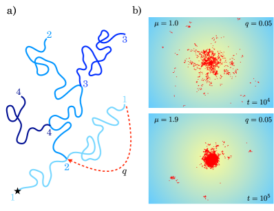
Figure 1: (Color online) a) Schematic view of a process relocating at a constant rate ($q$) to sites occupied at previous times, these times being chosen stochastically. The numbers label the beginning and end of each excursion. Each end is followed by the beginning of the next excursion (arrow). b) Two simulated trajectories corresponding to Lévy excursions with $p(\ell)\sim 1/|\ell|^{1+\mu}$, relocation rate $q=0.05$ and relocation kernel given by Eq. (8) [panels at the same scale].

III Random walks with relocations

We now consider a concrete class of non-Markovian walks for which the above ideas apply. The processes of interest are self-attracting, namely, they tend to revisit locations visited in the past. Particular examples were studied numerically in gautestad2005 ; gautestad2006 as animal movement models, or theoretically in solis ; romo . We present here a unified view of this class of processes.

Let $q$ be a parameter ($0<q<1$). At any time $t$, the walker chooses its next position according to the following rules:

(i) with probability $1-q$, it performs a random displacement $\ell$ drawn from a given distribution $p(\ell)$ like in standard random walks or Lévy flights;

(ii) with the complementary probability $q$, it jumps (or ’reset’) directly to the site occupied at some previous time $t^{\prime}\leq t$. The time $t^{\prime}$ is chosen according to a given probability $\pi_{t}(t^{\prime})$, or memory function, with $\sum_{t^{\prime}=0}^{t}\pi_{t}(t^{\prime})=1$ by normalization.

The rules are depicted in Fig. 1a, with two simulated examples in Fig. 1b. Note that in (ii), the next target site is chosen independently of its distance to the location $X_{t}$ of the walker. If $\pi_{t}(t^{\prime})=\delta_{t^{\prime},0}$, the site chosen for revisit is unique (the origin), a case which corresponds to the well-studied random walk with resetting to the origin evansmaj ; montero ; resetlevy ; nowak . For more general kernels, the walk is strongly path-dependent but still described by a master equation:

$$P(n,t+1)=(1-q)\sum_{\ell=-\infty}^{\infty}p(\ell)P(n-\ell,t)+q\sum_{t^{\prime}=0}^{t}\pi_{t}(t^{\prime})P(n,t^{\prime}).$$ (7)

Standard random walks or Lévy flights are recovered for $q=0$. If $q\neq 0$, the last term indicates that site $n$ can be chosen to be occupied at time $t+1$, provided it was visited at the earlier time $t^{\prime}$.

We first consider a uniform memory function, that is, independent of $t^{\prime}$:

$$\pi_{t}(t^{\prime})=\frac{1}{t+1}.$$ (8)

We call this case the preferential visit model (PVM): with such kernel, rule (ii) is simply equivalent to choosing a given site $n$ (among all visited sites) with probability proportional to the number of visits received by $n$ since $t=0$. Therefore the walker is prone to revisit familiar sites, at the expanse of rarely visited ones. The moments $\langle X_{t}^{2p}\rangle$ where calculated in solis for the PVM with nearest neighbor (n.n.) steps ($\ell_{i}=\pm 1$) in rule (i). To solve Eq. (7) more generally, we define the Laplace transform of $\widetilde{P}(k,t)$:

$$\widehat{P}(k,\lambda)=\sum_{t=0}^{\infty}\lambda^{t}\sum_{n=-\infty}^{\infty}e^{-ikn}P(n,t).$$ (9)

By taking the double transform of Eq. (7) with the kernel (8) and writing $\lambda^{t}/(t+1)=\lambda^{-1}\int_{0}^{\lambda}u^{t}du$, we obtain:

$$\widehat{P}(k,\lambda)-1=(1-q)\tilde{p}(k)\lambda\widehat{P}(k,\lambda)+q\int_{0}^{\lambda}du\frac{\widehat{P}(k,u)}{1-u}.$$ (10)

Taking the derivative of Eq. (10), one obtains a first-order ODE in the variable $\lambda$. As $P(n,t=0)=\delta_{0,n}$, the condition $\widehat{P}(k,0)=1$ must be enforced, leading to the exact solution:

$$\widehat{P}(k,\lambda)=(1-\lambda)^{-[1-a(k)]}\left[1-(1-q)\tilde{p}(k)\lambda\right]^{-a(k)}$$ (11)

with

$$a(k)=(1-q)\frac{1-\tilde{p}(k)}{1-(1-q)\tilde{p}(k)}.$$ (12)

We can infer the large $t$ behavior of $\widetilde{P}(k,t)$ by studying the divergence of $\widehat{P}(k,\lambda)$ near $\lambda=1$, with $k$ fixed but small. Noting that $a(k)\ll 1$, Eq. (11) yields $\widehat{P}(k,\lambda)\simeq(1-\lambda)^{-[1-a(k)]}$. This expression is simply inverted as:

$$\widetilde{P}(k,t)\simeq t^{-a(k)},$$ (13)

as announced in (5). In the absence of bias, one can use Eq. (2), which, combined with (12), gives the exponent:

$$a(k)\simeq\frac{1-q}{q}C|k|^{\mu},$$ (14)

implying the limit law (6). We conclude that this random walk always diffuses logarithmically, unlike other re-inforced walks that exhibit transitions to localized states davis ; grassberger . Numerical simulations confirm the very slow dynamics, even for $\mu<2$: a perfect agreement with the prediction $\langle|X_{t}|^{\nu}\rangle\sim(\ln t)^{\nu/\mu}$ for $\nu<\mu$ is observed in Fig. 2a. Importantly, the scaling function $f(x)$ in this non-Markovian process is the same as for the underlying Markovian process between relocations (or with $q=0$). This property stems from the fact that the cumulant characteristic function $\ln\tilde{p}(k)$ [Eq. (1)] and the function $a(k)$ [Eq.(12)] have the same leading behavior at small $k$, except for a multiplicative constant. In other words, the analyticity or non-analyticity of $\widetilde{P}(k,t)$ is preserved when $q$ is set different from zero.

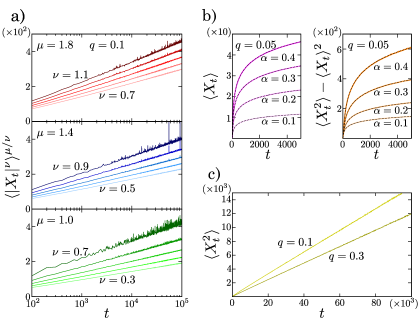
Figure 2: (Color online) Preferential visit model in $1d$. a) $\langle|X_{t}|^{\nu}\rangle^{\mu/\nu}$, obtained from simulations with different $\mu$ and $\nu$ (averages over $5\times 10^{5}$ runs), is proportional to $\ln t$ as expected. b) Mean and variance of $X_{t}$ for a n.n. walk with bias $\alpha$ in rule (i). Colored solid lines are simulations and dark dashed lines, theory. c) Normal diffusion for spatially uniform relocations.

IV Generalizations

We now show that several extensions of the PVM also admit a propagator of the form given by Eq. (5).

IV.1 Decaying memory

The results of the previous Section do not change qualitatively by considering memory kernels other than a pure preferential one. For instance, the time in the past $t^{\prime}$ may be chosen not uniformly like in Eq. (8) but with a probability decaying with $t-t^{\prime}$, the interval of time between a remembered occupation and the present time. Consider, for instance, a power-law memory decay:

$$\pi_{t}(t^{\prime})=\frac{(t-t^{\prime}+1)^{-\beta}}{\sum_{t^{\prime\prime}=0}^{t}(t-t^{\prime\prime}+1)^{-\beta}}$$ (15)

with $\beta>0$ an exponent. Here, the visits are still preferential, but with a tendency towards more recent sites (an effect actually observed in human mobility recency ). If $\beta<1$ the sum in (15) diverges at large $t$ and can be substituted by an integral; by taking the Fourier transform of (7) and making the ansatz $\widetilde{P}(k,t)\simeq t^{-a(k)}$, one obtains an integral equation for $a(k)$:

$$1-(1-q)\tilde{p}(k)=q(1-\beta)\int_{0}^{1}du(1-u)^{-\beta}u^{-a(k)}.$$ (16)

Combining Eqs. (16) and (2) gives, at small $k$:

$$a(k)\simeq\frac{1-q}{q}\ {\cal F}(\beta)C|k|^{\mu},$$ (17)

$${\rm with}\quad{\cal F}(\beta)=\left[(1-\beta)\int_{0}^{1}du(1-u)^{-\beta}\ln(1/u)\right]^{-1}.$$

Eq. (17) shows that the scaling law (6) applies to more general processes than the PVM. [Eq.(14) is recovered for $\beta=0$.] Interestingly, ${\cal F}(1)=\infty$, which indicates that the scaling form (5) breaks down for $\beta\geq 1$. Actually, a similar calculation to the one above shows that, for $\beta>2$, memory decays too fast to be relevant and the usual CLT (4) is recovered. Of course, these results do not mean that the aforementioned preservation property holds for arbitrary $\pi_{t}(t^{\prime})$. For instance, for memory walks with $1<\beta<2$ and steps $\ell_{i}$ of finite variance, the process is non-Gaussian romo . Likewise, Brownian random walks and Lévy flights subjected to stochastic reseting to the origin have asymptotic probability densities which are non-Gaussian evansmaj and non-Lévy nowak , respectively.

IV.2 Model with bias

We now study the response of the non-Markovian walks (at fixed $q$) to the presence of a constant forcing, namely, a bias $\alpha\equiv\langle\ell\rangle=\sum_{\ell=-\infty}^{\infty}\ell p(\ell)\neq 0$. Here, we assume $\langle\ell^{2}\rangle<\infty$ or $\mu=2$. By taking the first moment of Eq. (7), an equation for the average position $\langle X_{t}\rangle\equiv\sum_{n=-\infty}^{\infty}nP(n,t)$ is obtained:

$$\langle X_{t+1}\rangle=(1-q)[\langle X_{t}\rangle+\alpha]+q\sum_{t=0}^{t}\pi_{t}(t^{\prime})\langle X_{t^{\prime}}\rangle,$$ (18)

for any kernel $\pi_{t}(t^{\prime})$. We now denote $\langle X_{t}^{2}\rangle_{{}_{0}}$ as the mean square displacement of the walker at zero bias. It is easy to show that $\langle X_{t}^{2}\rangle_{{}_{0}}$ obeys exactly the same equation as (18), where $\alpha$ has to be replaced by $\langle\ell^{2}\rangle_{{}_{0}}=\sum_{\ell=-\infty}^{\infty}\ell^{2}p_{{}_{0}}(\ell)$, with $p_{{}_{0}}(\ell)$ unbiased. We deduce an Einstein fluctuation-dissipation relation (FDR):

$$\langle X_{t}\rangle=\frac{\alpha}{\langle\ell^{2}\rangle_{{}_{0}}}\langle X_{t}^{2}\rangle_{{}_{0}}$$ (19)

The exact equality (19) is general: it is valid at all $t$ and for any kernel $\pi_{t}(t^{\prime})$ (allowing to recover results on the resetting to the origin with bias montero ). Despite of being out-of-equilibrium, the FDR with constant bias in this system is the same as for ordinary random walks, where the response $\langle X_{t}\rangle$ is entirely determined by the fluctuations at zero bias. With the kernel (15) and $\beta<1$, the drift is thus logarithmic: $\langle X_{t}\rangle\simeq\alpha\frac{1-q}{q}{\cal F}(\beta)\ln t$, from Eqs. (19) and (17) with $\mu=2$. The time evolution of the first moment $\langle X_{t}\rangle$ is displayed in Fig.2b-left for different parameter values.

In other words, the effective friction coefficient of the walker ($\propto\alpha\langle\dot{X}_{t}\rangle^{-1}$) grows linearly with $t$. This illustrates the non-stationarity emerging from long range memory and the increasingly sluggish dynamics caused by frequent relocations to the same preferred sites.

We further show that the combination of memory and bias has a drastic impact on the fluctuations of $X_{t}$ around $\langle X_{t}\rangle$. We take, for example, the PVM with n.n. steps in rule (i), and expand Eq. (12), which is valid for any $p(\ell)$, near $k=0$. Now using $\tilde{p}(k)=1-i\alpha k-\frac{1}{2}k^{2}+...$ we obtain $\widetilde{P}(k,t)\simeq\exp[-i\mu_{t}k-\frac{1}{2}\sigma_{t}k^{2}]$, which corresponds for $P(n,t)$ to a Gaussian of mean $\mu_{t}$ and variance $\sigma_{t}$. We recover $\mu_{t}=\alpha\frac{1-q}{q}\ln t$, see (19), and obtain for $\sigma_{t}$:

$$\sigma_{t}=\left[\frac{1-q}{q}+2\left(\frac{1-q}{q}\right)^{2}\alpha^{2}\right]\ln t.$$ (20)

If $q$ is small, the presence of a bias therefore strongly amplifies the fluctuations of $X_{t}$, as the 2^nd term in (20) is $>0$ and dominant. This effect is displayed in Fig. 2b-right. For ordinary n.n. random walks, on the contrary, the bias decreases the fluctuations: in that case $\sigma_{t}=(1-\alpha^{2})t$ and motion becomes deterministic at $\alpha=1$ (see e.g. gleb ).

V Discussion and conclusion

In summary, we have shown that Lévy and Gaussian distributions can emerge generically far from the domain of applicability of the CLT, namely, in strongly subdiffusive path-dependent processes. We emphasize that the processes studied here exhibit subdiffusion because the relocation sites are selected heterogeneously in space. This situation is also encountered in the reseting to the origin, an extreme case where only one site receives all relocations, causing the typical diffusion length $l(t)$ to tend to a constant evansmaj . To illustrate the importance of uneven relocations, one may by contrast consider a n.n. random walk, which, in rule (ii) above, relocates to a site chosen randomly and uniformly among the visited sites. In this case, $l(t)$ roughly obeys $dl/dt\sim(2R/l)[(R/2)/(1/q)]$, with $R=\sqrt{2D/q}$ the characteristic diffusion scale between two relocations, $2R/l$ being the probability of reseting near the edges of the territory covered by the walk. This leads to $l(t)\sim\sqrt{4Dt}$, a normal diffusive behavior, which is qualitatively confirmed by the numerical simulations of Figure 2c.

The emergence of logarithmic diffusion can be understood qualitatively by drawing, from Fig. 1a, an analogy with a branching random walk (see, e.g. biggins ; branchsatya ). Consider an initial normal random walk with a constant branching rate $q_{b}$. At each branching event, a new random walk is created which starts from the current position of the parent walk. The walks are independent, do not disappear, and all branch at the same rate $q_{b}$. The process follows until it is stopped at some final time $T$. Let then imagine a single walker starting at the origin and following the paths left by all the branches, from the oldest to most recent, relocating at the start of the next branch when reaching the end of a branch. The average number of branches at time $T$ is $N_{b}(T)=e^{q_{b}T}$ and the total number of steps needed for the single walker to walk along all of them is $t\simeq\int_{0}^{T}d\tau N_{b}(\tau)\simeq e^{q_{b}T}/q_{b}$. At time $t$, the single walker will be at a typical distance $l(t)$ from the origin, with $l(t)^{2}\sim T\simeq\frac{1}{q_{b}}\ln t$. This form is surprisingly similar to our result $\langle X_{t}^{2}\rangle\simeq\frac{1}{q}\ln t$ for the PVM at small $q$. The argument above can be repeated with branching Lévy flights, where $l(t)\propto T^{1/\mu}$, leading to a similar correspondence between the two models.

Note that the above analogy is only qualitative, as the PVM differs quantitatively from a set of branching RWs. Setting $q_{b}=q$, numerical simulations (not shown) indicate that, due to the rule of preferential visits, the relocation points in the memory model are distributed much more heterogeneously in space (namely, closer to the origin) than the branching points of the branching walks.

We conclude by mentioning that the processes studied here can explain two properties very often observed in human and animal mobility gab ; rhee ; gonzalez ; song ; solis : a) power-law distributed step lengths can coexist with a very slow diffusion in the long term (i.e., home range behavior); b) the occupation of space by an individual within its home range is very non-uniform. Lévy flights with relocations to visited places are likely to be an efficient strategy for searching and exploiting renewable resources, a challenge faced by many living organisms gandhi ; randomsearch ; benichou ; hills .

- (1) W. Feller, An Introduction to Probability Theory and its Applications, Vol. 2 (Wiley, New York, 2008).
- (2) G. Samoradnitsky and M. S. Taqqu, Stable Non-Gaussian Random Processes: Stochastic Models with Infinite Variance (Chapman Hall, 1994).
- (3) F. Bardou, J.-P. Bouchaud, A. Aspect, and C. Cohen-Tannoudji, Lévy Statistics and Laser Cooling (Cambridge, 2002).
- (4) P. Barthelemy, J. Bertolotti, and D. S. Wiersma, Nature 453, 495 (2008).
- (5) M. F. Shlesinger, G. M. Zaslavsky, and J. Klafter, Nature 363, 31 (1993).
- (6) J.-P. Bouchaud and A. Georges, Phys. Rep. 195, 127 (1990).
- (7) A. V. Chechkin, R. Metzler, J. Klafter, and V. Yu. Gonchar, in Anomalous Transport: Foundations and Applications, edited by R. Klages, G. Radons, and I. M. Sokolov (Wiley-VCH Verlag, Weinheim, 2008), pp. 129–159.
- (8) R. Metzler and J. Klafter, Phys. Rep. 339, 1 (2000).
- (9) G. H. Weiss, Aspect and Applications of the Random Walk (Elsevier, Amsterdam, 1994).
- (10) V. Zaburdaev, S. Denisov, and J. Klafter, Rev. Mod. Phys. 87, 483 (2015).
- (11) T. H. Harris et al., Nature 486, 545 (2012).
- (12) G. M. Viswanathan, S. V. Buldyrev, S. Havlin, M. G. E. da Luz, E. P. Raposo, and H. E. Stanley, Nature 401, 911 (1999).
- (13) F. Bartumeus, M. G. E. da Luz, G. M. Viswanathan, and J. Catalan, Ecology 86, 3078 (2005).
- (14) D. W. Sims et al., Nature 451, 1098 (2008).
- (15) G. Ramos-Fernández, J. L. Mateos, O. Miramontes, G. Cocho, H. Larralde, and B. Ayala-Orozco, Behav. Ecol. Sociobiol. 55, 223 (2004).
- (16) C. T. Brown, L. S. Liebovitch, and R. Glendon, Hum. Ecol. 35, 129 (2007).
- (17) D. A. Raichlen, B. M. Wood, A. D. Gordon, A. Z. P. Mabulla, F. W. Marlowe, and H. Pontzer, Proc. Natl. Acad. Sci. USA 111, 728 (2014).
- (18) D. Brockmann, L. Hufnagel, and T. Geisel, Nature 439, 462 (2006).
- (19) I. Rhee, M. Shin, S. Hong, K. Lee, and S. Chong, In Proc. IEEE INFOCOM, 13-18 April 2008, Phoenix, AZ (IEEE, Piscataway, NJ, 2008), pp. 924-932.
- (20) M. C. González, C. A. Hidalgo, and A.-L. Barabási, Nature 453, 779 (2008).
- (21) C. Song, T. Koren, P. Wang, and A.-L. Barabási, Nature Phys. 6, 818 (2010).
- (22) A. O. Gautestad and I. Mysterud, Am. Nat. 165, 44 (2005).
- (23) A. O. Gautestad and I. Mysterud, Ecol. Complex. 3, 44 (2006).
- (24) L. Brger, B. D. Dalziel, and J. M. Fryxell, Ecol. Lett. 11, 637 (2008).
- (25) D. Boyer and C. Solis-Salas, Phys. Rev. Lett. 112, 240601 (2014).
- (26) S. I. Denisov and H. Kantz, Phys. Rev. E 83, 041132 (2011).
- (27) J. Drger and J. Klafter, Phys. Rev. Lett. 84, 5998 (2000); R. Venegeroles, J Stat Phys 154, 988 (2014).
- (28) J. Klafter and I. M. Sokolov, First Steps in Random Walks (Oxford, Oxford, 2011).
- (29) W. F. Fagan et al., Ecol. Lett. 16, 1316 (2013).
- (30) B. van Moorter et al., Oikos 118, 641 (2009).
- (31) M. Magdziarz and A. Weron, Phys. Rev. E 75, 056702 (2007).
- (32) H. J. Hilhorst, Braz. J. Phys. 39, 371 (2009).
- (33) G. M. Schtz and S. Trimper, Phys. Rev. E 70, 045101(R) (2004).
- (34) N. Kumar, U. Harbola, and K. Lindenberg, Phys. Rev. E 82, 021101 (2010).
- (35) M. A. A. da Silva, G. M. Viswanathan, and J. C. Cressoni, Phys. Rev. E 89, 052110 (2014).
- (36) B. Davis, Probab. Theor. Related Fields 84, 203 (1990).
- (37) E. Bolthausen and U. Schmock, Ann. Probab. 25, 531 (1997).
- (38) V. B. Sapozhdcov, J. Phys. A: Math. Gen. 27, L151 (1994).
- (39) J. G. Foster, P. Grassberger, and M. Paczuski, New J. Phys. 11, 023009 (2009).
- (40) H. G. Othmer and A. Stevens, SIAM J. Appl. Math. 57, 1044 (1997).
- (41) S. C. Lim and S. V. Muniandy, Phys. Rev. E 66, 021114 (2002).
- (42) A. S. Bodrova, A. V. Chechkin, A. G. Cherstvy, and R. Metzler, New J. Phys. 17, 063038 (2015).
- (43) M. Vendruscolo and M. Marsili, Phys. Rev. E 54, R1021 (1996).
- (44) M. Schmiedeberg, V. Y. Zaburdaev, and H. Stark, J. Stat. Mech. P12020 (2009).
- (45) E. Barkai, V. Fleurov, and J. Klafter, Phys. Rev. E 61, 1164 (2000).
- (46) D. Boyer and J. C. R. Romo-Cruz, Phys. Rev. E 90, 042136 (2014).
- (47) M. R. Evans and S. N. Majumdar, Phys. Rev. Lett. 106, 160601 (2011); J. Phys. A: Math. Theor. 44, 435001 (2011).
- (48) M. Montero and J. Villarroel, Phys. Rev. E 87, 012116 (2013).
- (49) L. Kuśmierz, S. N. Majumdar, S. Sabhapandit, and G. Schehr, Phys. Rev. Lett. 113, 220602 (2014).
- (50) L. Kuśmierz and E. Gudowska-Nowak, Phys. Rev. E 92, 052127 (2015).
- (51) H. Barbosa, F. Buarque de Lima Neto, A. Evsukoff, and R. Menezes, arXiv:1504.01442 [physics.soc-ph] (2015).
- (52) O. Bénichou, K. Lindenberg, and G. Oshanin, Phys. A 392, 3909 (2013).
- (53) J.D. Biggins, Stochastic Process. Appl. 34, 255 (1990).
- (54) K. Ramola, S. N. Majumdar, and G. Schehr, Chaos Soliton. Fract. 74, 79 (2015).
- (55) O. Bénichou, C. Loverdo, M. Moreau, and R. Voituriez, Rev. Mod. Phys. 83, 81 (2011).
- (56) G. M. Viswanathan, M. G. E. da Luz, E. P. Raposo, and H. E. Stanley, The Physics of foraging (Cambridge, Cambridge, 2011).
- (57) T. T. Hills, P. M. Todd, D. Lazer, A. D. Redish, and I. D. Couzin, Trends Cogn. Sci. 19, 46 (2015).