Image Classification with Rejection using Contextual Information

Abstract

We introduce a new supervised algorithm for image classification with rejection using multiscale contextual information. Rejection is desired in image-classification applications that require a robust classifier but not the classification of the entire image. The proposed algorithm combines local and multiscale contextual information with rejection, improving the classification performance.

As a probabilistic model for classification, we adopt a multinomial logistic regression. The concept of rejection with contextual information is implemented by modeling the classification problem as an energy minimization problem over a graph representing local and multiscale similarities of the image. The rejection is introduced through an energy data term associated with the classification risk and the contextual information through an energy smoothness term associated with the local and multiscale similarities within the image. We illustrate the proposed method on the classification of images of H&E-stained teratoma tissues.

I Introduction

In many classification problems, the cost of creating a training set that is statistically representative of the input dataset is often high. This is due to the required size of the training set, and the difficulty of obtaining a correct labeling resulting from unclear class separability and the possibility of presence of unknown classes. In this work, we were motivated by the need for automated tissue identification (classification) in images from Hematoxylin and Eosin (H&E) stained histopathological slides [1, 2, 3, 4]. H&E staining is used both for diagnosis as well as to gain a better understanding of the diseases and their processes, consisting of the sequential staining of a tissue with two different stains that have different affinities to different tissue components.

In this paper, we are interested in a subclass of image classification problems with the following characteristics:

• The classification is not directly based on the observation of pixel values but on higher-level features;

• The characteristics of the image make it impossible to have access to pixelwise ground truth, leading to small, unbalanced, noisy, or incomplete training sets;

• The pixels may belong to unknown classes;

• The classification accuracy at pixels belonging to interesting or known classes is more important than the classification accuracy at pixels belonging to uninteresting or unknown classes;

• The need for high accuracy surpasses the need to classify all the samples.

I-A Goal

In problems as above, introducing a rejection yields improvements in the classification performance — classification with rejection. Further improvements in accuracy can be obtained by exploiting spatial and multilevel similarities — classification using contextual information. Our goal is to combine classification with rejection and classification using contextual information in an image classification framework to obtain improved classification performance.

I-B Classification with Rejection

A classifier with rejection can be seen as a coupling of two classifiers: (1) a general classifier that classifies a sample and (2) a binary classifier that, based on the information available as input and output of the first classifier, decides whether the classification performed by the first classifier was correct or incorrect. As a result, we are able to classify according to the general classifier, or reject if the decision of the binary classifier is that the former classification is incorrect.

A classifier with rejection allows for coping with unknown information and reducing the effect of nonideal training sets. It was first analyzed in [5], where Chow’s rule for optimum error-reject trade-off was presented. Based on the posterior probabilities of the classes given the features for the classification, Chow’s rule allows for the determination of a threshold for rejection, such that the classification risk is minimized. The authors in [6] point out that Chow’s rule only provides the optimal error-reject threshold if these posterior probabilities are exactly known. They propose the combination of class-related reject thresholds to improve the error-reject trade-off. Parameters are selected using the constrained maximization of the accuracy subject to upper bounds on the rejection rate as a performance metric. In [7], the authors present a mathematical framework for binary classification with rejection. In that approach, the rejection is based on risk minimization and the cost for each different binary classification error considered.

Usually, the rejection is applied as a plug-in rule to the outputs of a classifier. It is also possible, however, to combine the output of multiple classifiers (multiple general classifiers) to create rejection. In [8], the authors present a multi-expert system based on a Bayesian combination rule. The reliability of the classification is estimated from the posterior probabilities of the two most probable classes, and the rejection works by thresholding the reliabilities.

Another approach is to include the rejection in the classifier itself as an embedded rejection instead of a plug-in rule. In [9], the rejection is embedded in a Support Vector Machine (SVM), in which the rejection is present in the training phase of the SVM and included in the formulation in close association with the separating hyperplane resulting from the SVM. This leads to a nonconvex optimization problem that can be approximately solved by finding a surrogate loss function. In [10] and [11], the statistical properties of a surrogate loss function are studied and applied to the task of rejection by risk minimization. In [12], the use of LASSO-type penalty for risk minimization is analyzed.

Yet another approach consists in having a second classifier with access to the input and output of the first classifier instead of a plug-in rule or an embedded rejection. In [13], the second classifier is trained with the main classifier to assess the reliability of the main classifier. The rejection is based on thresholding the reliability provided by the second classifier.

More recently, in [14], the authors present a framework for the multilabel classification problem with rejection. A trade-off between the accuracy of the nonrejected samples and the rejection cost is found as a result of a constrained optimization problem. Furthermore, an application-specific reliability measure of the classification with rejection inspired on the F-score (weighted harmonic mean of precision and recall) is defined.

In the present work, we propose a classification system with rejection using contextual information. To assess the performance of the method, in addition to the fraction of rejected samples $r$ and the classification accuracy on the subset of nonrejected samples $A$, we use the concept of classification quality $Q$ and rejection quality $\phi$ [15]. The classification quality can be defined as the accuracy of a binary classifier that aims to classify correctly classified samples as nonrejected and incorrectly classified samples as rejected. Maximizing the classification quality leads both to keeping correctly classified samples and rejecting incorrectly classified samples. The classification quality allows us to compare different classifiers with different rejection ratios and accuracies. The rejection quality can be defined as the positive likelihood ratio of a binary classifier that aims to classify correctly classified samples as nonrejected and incorrectly classified samples as rejected. It compares the proportion of correctly classified to incorrectly classified samples in the set of rejected samples to the proportion on the entire data. The rejection quality provides insight into the ability of a classifier with rejection to concentrate incorrectly classified samples in the set of rejected samples.

I-C Classification with Contextual Information

The basic assumption for classification with contextual information is that the data is not spatially independent: in most real-world data, two neighboring pixels are likely to belong to the same class. This assumption can be extended to include multiple definitions of a neighborhood: local, nonlocal, and multiscale.

The use of contextual information is prevalent in tasks in which the spatial dependencies play an important role, such as image segmentation and image reconstruction [16]. In [17], the authors formulate a discriminative framework for image classification taking in account spatial dependencies. This framework allows both the use of discriminative probabilistic models and adaptive spatial dependencies.

For the purposes of our application, we can learn from hyperspectral image classification, where the use of of contextual information is prevalent [18, 19]. We model classification with contextual information as a Discriminative Random Field (DRF) [17] with the association potential linked with the pixelwise class posterior probabilities and the interaction potential linked with a multilevel logistic (MLL) Markov random field (MRF) [20] endowed with a neighboring system associated with a multi-scale similarity graph. This MLL-MRF promotes segmentations in which neighboring samples are likely to belong to the same class at multiple scales, leading to multi-scale spatial consistency among the classifications.

I-D Classification with Rejection Using Contextual Information

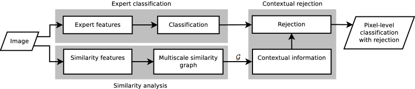
Figure 1: Classification with rejection using contextual information. Each gray block is discussed in a separate section: similarity analysis in Section III, expert classification in Section IV, and contextual rejection in Section V.

The proposed framework, shown in Fig. 1, combines classification with rejection with classification with contextual information. Our approach allows for not only rejecting a sample when the information is insufficient to classify, but also for not rejecting a sample when an ”educated guess” is possible based on neighboring labels (local and nonlocal from the spatial point of view). We do so by transforming the soft classification (posterior distributions) obtained by an expert classifier into a hard classification (labels) that considers both rejection and contextual information.

An expert classifier is designed based on application-specific features and a similarity graph is constructed representing the underlying multiscale structure of the data. The classification risk from the expert classifier is computed and the rejection is introduced as a simple classification risk threshold rule in an extended risk formulation. This formulation consists in a maximum a posteriori (MAP) inference problem defined on the similarity graph, thus combining rejection and contextual information.

Compared with classification with rejection only, our approach has an extra degree of complexity: the rejection depends not only on a rejection threshold for the classification but also on a rejection consistency parameter. By imposing a higher rejection consistency, the rejected samples become rejection areas (that is, a nonrejected sample surrounded by rejected samples will tend to be rejected too), which is meaningful in the task of image classification.

Compared with classification with contextual information only, this problem is of the same complexity, as the rejection can be treated as a class, and class-specific transitions can be easily modeled.

I-E Outline of the Paper

In Section II, we describe the background for our framework: partitioning, feature extraction, and classification. In Section III, we explore the similarity analysis block of the framework and the design of a multilevel similarity graph that represents the underlying structure of the data. In Section IV, we describe the elements of the expert classification block of the framework not described on the background. We introduce the rejection as a mechanism for handling the inability of the classifier to correctly classify all the samples. In Section V, we combine the expert classification and the multiscale similarity graph in an energy minimization formulation to obtain classification with rejection using contextual information. In Section VI, we apply our framework to classification of real data: natural images, and H&E-stained teratoma tissue images. Finally, Section VII concludes the paper.

II Background

We now describe the background for our work in terms of image partitioning, features, classification, and methods used to compute the MAP solution.

Let $\mathcal{S}=\{1,\ldots,s\}$ denote the set of pixel locations, $\mathbf{z}_{i}\in\mathbb{R}^{d}$ denote an observed vector at pixel $i\in{\cal S}$, $I=[\mathbf{z}_{1},\mathbf{z}_{2},\dots,\mathbf{z}_{s}]\in\mathbb{R}^{d\times s}$ denote an observed image, $P=\{\mathbf{x}_{1},\ldots,\mathbf{x}_{n}\}$ denote a partition of $\cal S$, $\mathcal{V}=\{1,\ldots,n\}$ denote a set indexing the elements of the partition $P$ termed superpixels, and $\mathcal{E}=\mathcal{V}\times\mathcal{V}$ denote a set indexing pairs of neighboring superpixels. Given that $P$ is a partition of $\cal S$, then $\mathbf{x}_{i}\subset{\cal S}$, for $i\in\cal N$, $\mathbf{x}_{i}\cap\mathbf{x}_{j}=\emptyset$ for $i\neq j\in\cal N$, and $\cup_{i=1}^{n}\mathbf{x}_{i}=\mathcal{S}$.

II-A Partitioning

To decrease the dimensionality of the problem, and thus the computational burden, we partition the set of pixel locations $\cal S$ into a partition $P$, allowing for the efficient use of graph-based methods. The partitioning of the image is performed by oversegmentation creating superpixels as described in . This method, as is typical in most segmentation techniques, aims at maintaining a high level of similarity inside each superpixel and high dissimilarity between different superpixels.

Because of how the superpixels are created (measuring the evidence of a boundary between two regions), there is a high degree of inner similarity in each partition element; the elements of a superpixel will very likely belong to the same class. The major drawback of using this partitioning method is that the partition elements are highly nonuniform in terms of size and shape.

II-B Features

We use two kinds of features: (1) application-specific features encode expert knowledge and are used to classify each partition element, and (2) generic similarity features represent low-level similarities of the image and are used to assess the similarity among the partition elements. From each partition element $\mathbf{x}_{i}$, we extract statistics of the application-specific features and of the similarity features (from all pixels belonging to the same partition element), mapping from features defined on an image pixel space to features defined on an image partition space.

II-C Classification

Given the partition $P$ and the associated feature matrix $\mathbf{F}=[\mathbf{f}_{1},\ldots,\mathbf{f}_{n}]$, with $\mathbf{f}_{i}\in\mathbb{R}^{m}$ the $m$-dimentional application-specific features , we wish to classify each partition element $\mathbf{x}_{i}\in P$ into a single class. We do so by assigning to it a label $y_{i}\in\mathcal{L}=\{1,\ldots,N\}$ representative of its class. This assignment is performed by maximizing the posterior distribution $p(\mathbf{y}|\mathbf{F})$ with respect to $\mathbf{y}=[y_{1},\dots,y_{n}]$, that is, by computing MAP labeling

$$\hat{\mathbf{y}}\in\arg\max_{\mathbf{y}\in{\cal L}^{n}}p(\mathbf{y}|\mathbf{F}).$$ (1)

We note that under the assumption of conditional independence of features given the labels $p(\mathbf{y}|\mathbf{F})=\prod_{i\in\mathcal{S}}p(y_{i}|\mathbf{f}_{i})$ and of equiprobable class probabilities $p(y_{i})=p(y_{j})$, for all $i,j\in\mathcal{S}$, we can reformulate the MAP formulation in (1) as

$$\hat{\mathbf{y}}\in\arg\min_{\mathbf{y}\in{\cal L}^{n}}\sum_{i\in\mathcal{S}}-\log p(y_{i}|\mathbf{f}_{i})-\log p(\mathbf{y}).$$ (2)

For the posterior $p(\mathbf{y}|\mathbf{F})$ we adopt the DRF model [17],

$$\begin{split}p(\mathbf{y}|\mathbf{F})\propto\exp\bigg{(}-(1-\alpha)\sum_{i\in\cal V}D(y_{i},\mathbf{f}_{i})\\ -\alpha\sum_{\{i,j\}\in\cal E}V_{\{i,j\}}(y_{i},y_{j})\bigg{)},\end{split}$$ (3)

where $-D(y_{i},\mathbf{f}_{i})$ is the association potential, which links discriminatively the label $y_{i}$ with the feature vector $\mathbf{f}_{i}$, $-V_{\{i,j\}}(y_{i},y_{j})$ is the interaction potential, which models the spatial contextual information, and $\alpha\in[0,1]$ is a regularization parameter that controls the relative weight of the two potentials. The posterior (3) is a particular case of the DRF class introduced in [17], because the association potential does not depend on the partition elements. The DRF model used constitutes an excellent trade-off between model complexity and goodness of the inferences, as shown in Section VI.

To completely define (3), we need to specify the association potential $-D$ and the interaction potential $-V_{\{i,j\}}$. In this work, we start from the assumption that $-D(y_{i},\mathbf{f}_{i})=\log p(y_{i}|\mathbf{f}_{i},{\mathbf{W}})$, resulting from (2) and (3), where $p(y_{i}|\mathbf{f}_{i},{\mathbf{W}})$ is the multinomial logistic regression (MLR) [21] parameterized with the matrix of regression coefficients ${\mathbf{W}}$, $-V_{\{i,j\}}(y_{i},y_{j})=w_{ij}\delta_{y_{i},y_{j}}$, where $w_{ij}\geq 0$ is a weight to be defined late,r and $\delta_{i,j}$ is the Kronecker symbol (i.e., $\delta_{i,j}=1$ if $i=j$ and $\delta_{i,j}=0$ if $i\neq j$). This class of association potentials, which define a MLL-MRF prior [20], promotes neighboring labels of the same class. In the following subsection we address the learning of the MLR regression matrix ${\mathbf{W}}$ detail.

II-C1 Multinomial Logistic Regression

Let $k(\mathbf{f})=[k_{0}(\mathbf{f}),\ldots,k_{q}(\mathbf{f})]^{T}$ denote a vector of nonlinear functions $k_{i}:\mathbb{R}^{m}\rightarrow\mathbb{R}$, for $i=0,\dots,q$, with $q$ the number of training samples and with $k_{0}=1$. The MLR models the a posteriori probability of $y_{i}\in\cal L$ given $\mathbf{f}\in\mathbb{R}^{m}$ as

$$p(y_{i}=l|\mathbf{f},{\mathbf{W}})=\frac{e^{\mathbf{w}_{l}^{T}k(\mathbf{f})}}{\sum_{j=1}^{N}e^{\mathbf{w}_{j}^{T}k(\mathbf{f})}},$$ (4)

where ${\mathbf{W}}=[\mathbf{w}_{1},\dots,\mathbf{w}_{N}]\in\mathbb{R}^{(q+1)\times N}$ the matrix of regression coefficients. Given that $p(y_{i}|\mathbf{f},{\mathbf{W}})$ is invariant with respect to a common translation of the columns of ${\mathbf{W}}$, we arbitrarily set $\mathbf{w}_{N}=0$.

II-C2 Learning the Regression Coefficients $W$

Our approach is supervised; we can thus split the dataset into a training set ${\cal D}=\{(y_{i},\mathbf{f}_{i}),\,i\in{\cal T}\}$, where ${\cal T}\subset\cal V$ is a set indexing the labeled superpixels, and the set $\{\mathbf{f}_{i},\,i\in{\cal V-T}\}$ containing the remaining unlabeled feature vectors. Based on these two sets and on the DRF model (3), we can infer matrix ${\mathbf{W}}$ jointly with the MAP labeling $\hat{\mathbf{y}}$. Because it is difficult to compute the normalizing constant of $p(\mathbf{y}|\mathbf{F})$, this procedure is complex and computationally expensive.

Aiming at a lighter procedure to learn the matrix ${\mathbf{W}}$, we adopt the sparse multinomial logistic regression (SMLR) criterion introduced in [22], which, fundamentally, consists in setting $\alpha=0$ in (3), that is, disconnecting the interaction potential, and computing the MAP estimate of ${\mathbf{W}}$ based on the training set ${\cal D}$ and on a Laplacian independent and identically distributed prior for the components of ${\mathbf{W}}$. We are then led to the optimization

$$\widehat{{\mathbf{W}}}\in\arg\max_{W}\,\,l({\mathbf{W}})+\log p({\mathbf{W}}),$$ (5)

with $l({\mathbf{W}})=\sum_{i\in\cal T}\log p(y_{i}|\mathbf{f}_{i},{\mathbf{W}})$ the log-likelihood, and $p({\mathbf{W}})\propto e^{-\lambda\|{\mathbf{W}}\|_{1,1}}$ the prior, where $\lambda$ is the regularization parameter and $\|{\mathbf{W}}\|_{1,1}$ denotes the sum of the $\ell_{1}$ norm of the columns of the matrix ${\mathbf{W}}$. The prior $p({\mathbf{W}})$ promotes sparsity on the components of ${\mathbf{W}}$. It is well known that the Laplacian prior (the $\ell_{1}$ regularizer in the regularization framework) promotes sparse matrices ${\mathbf{W}}$, that is, matrices ${\mathbf{W}}$ with most elements set to zero. The sparsity of ${\mathbf{W}}$ avoids overfitting and thus improves the generalization capability of the MLR, mainly when the size of the training set is small [22]. The sparsity level is controlled by the parameter $\lambda$.

II-C3 LORSAL

We use the logistic regression via variable splitting and augmented Lagrangian (LORSAL) algorithm (see [18]) to solve the optimization (5). The algorithm is quite effective from the computational point of view, mainly when the dimension of $k\in\mathbb{R}^{q+1}$ is large.

LORSAL solves the equivalent problem

$$\min_{{\mathbf{W}},\mathbf{\Omega}}-l({\mathbf{W}})+\lambda||\mathbf{\Omega}||_{1,1},\quad\textrm{subject to:}\quad{\mathbf{W}}=\mathbf{\Omega}$$ (6)

The formulation in (6) differs from the one in (5) in the sense that $\log p({\mathbf{W}})$ is replaced by $\log p(\mathbf{\Omega})$ with the constraint ${\mathbf{W}}=\mathbf{\Omega}$ added to the optimization problem, introducing a variable splitting. Note that $-l({\mathbf{W}})$ is convex but nonquadratic, and $\lambda||\mathbf{\Omega}||_{1,1}$ is convex but nonsmooth, thus yielding a convex nonsmooth and nonquadratic optimization. LORSAL approximates $l({\mathbf{W}})$ by a quadratic upper bound [21], transforming the nonsmooth convex minimization (6) into a sequence of $\ell_{2}$-$\ell_{1}$ minimization problems solved with the alternating direction method of multipliers [23].

Given a set of indices corresponding to the training samples $\mathcal{T}$ and its respective training set $\mathcal{F}_{\mathcal{T}}=\{\mathbf{F}_{j}\}_{\{j\in\mathcal{T}\}}$, a radial basis function (RBF) is a possible choice of function in the vector of nonlinear regression function $k$ used in (4), which allows us to obtain a training kernel (computed by a RBF kernel of the training data). This allows us to deal with features that are not linearly separable. To normalize the values of the nonlinear regression function, the bandwidth of the RBF kernel is set to be the square root of the average of the distance matrix between the training and test sets. With both the regressor matrix ${\mathbf{W}}$ and the nonlinear regression function $k$ defined, we obtain the class probabilities from the MLR formulation in (4).

II-D Computing the MAP Labeling

From (3), we can write the MAP labeling optimization as

$$\arg\min_{\mathbf{y}\in{\cal L}^{n}}\,\,(1-\alpha)\sum_{i\in\cal V}D(y_{i})+\alpha\sum_{\{i,j\}\in\mathcal{E}}V_{\{i,j\}}(y_{i},y_{j}).$$ (7)

This is an integer optimization problem, which is NP-hard for most interaction potentials promoting piecewise smooth segmentations. A remarkable exception is the binary case (when $N=2$) and submodular interaction potentials, which are the interaction potentials that we consider; in this case the exact label can be computed in polynomial time by mapping the problem onto suitable graph and computing a min-cut/max-flow on that graph [24].

We find an approximate solution to this problem by using the $\alpha$-expansion algorithm [16, 25]. With the constraint that $V_{\{i,j\}}$ is metric in the label space, the local minimum found by $\alpha$-expansion is within a known factor of the global minimum of the labeling.

III Similarity Analysis

Similarity analysis is the first step (see Fig. 1) of the proposed approach. To represent similarities in the image, we construct a similarity multiscale graph by (a) partitioning the image at different scales and (b) finding both local and multiscale similarities. The partitioning of the image at each scale is computed from the oversegmentation that results from using superpixels [26]. The different scales used for partitioning reflect a compromise between computational cost associated with large multiscale graphs, and the performance gains achieved by having a multiscale graph that correctly represents the problem. The construction of a similarity multiscale graph (as exemplified in Fig. 2) allows us to encode local similarities at the same scale, and similarities at different scales. The edges of the similarity multiscale graph define the cliques present in (3). This knowledge can be used to improve the performance of the classification, as neighboring and similar partitions are likely to belong to the same class.

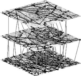
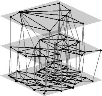
(a) Multiscale graph	(b) Multiscale graph
and multiscale partitioning	structure

Figure 2: Multiscale graph superimposed on the result of partitioning the same image at different scales (a) and on planes denoting the different scales (b). Nodes are denoted by circles, intrascale edges by gray lines, and interscale edges by black lines.

III-A Multiscale Superpixels

We obtain a multiscale partitioning of the image by computing superpixels at different scales, that is, selecting increasing minimum superpixel sizes (MSS) for each superpixelization. This leads to multiple partitions on which the minimum number of pixels in each partition element is changed, corresponding to a scale of the partition. The scale selection must achieve a balance between spatial resolution and representative partition elements (with sufficient size to compute the statistics on the features).

III-B Design of the Similarity Multiscale Graph

The design of the similarity multiscale graph is performed in three steps: (1) compute a graph for each single scale partition; (2) connect the single scale partition graphs; and (3) compute similarity-based edge weight assignment and prune edges. The main idea is that a partition will have an associated graph. By combining partitions with different scales (an inverse relation exists between the number of elements of a partition of an image and the scale associated with that partition), we are able to combine graphs with different scales. This will be the core of the similarity multiscale graph.

III-B1 Single Scale Graph as a Subgraph of the Multiscale Graph

Let us consider $P_{s}(I)=\bigcup_{i}\{\mathbf{x}^{s}_{i}\}$, the set of partition elements $\mathbf{x}^{s}_{i}$ obtained by partitioning of the image $I$ at scale $s$. We associate a node $n^{s}_{i}$ to each partition element $\mathbf{x}^{s}_{i}\in P_{s}(I)$ and defined the set of nodes at scale $s$ as

$$\mathcal{V}_{s}=\bigcup_{i}\{n^{s}_{i}\}.$$

There is a one-to-one correspondence between partition elements $\mathbf{x}^{s}_{i}$ and nodes $n^{s}_{i}$. For each pair of adjoint partition elements (partition elements that share at least one pixel at their boundary) at scale $s$, $(\mathbf{x}^{s}_{i},\mathbf{x}^{s}_{j})$, we create an undirected edge between the corresponding nodes. We have that the set of intrascale edges at scale $s$ is

$$\mathcal{E}_{s}=\bigcup_{i}\bigcup_{j\in\mathcal{N}(n^{s}_{i})}\{(n^{s}_{i},n^{s}_{j})\},$$

where $\mathcal{N}^{s}(n^{s}_{i})$ is the set of neighbor nodes of $n^{s}_{i}$, that is, the set of nodes that correspond to the partitions adjoint to the partition $\mathbf{x}^{s}_{i}$. Let $\mathcal{G}_{s}=\left(\mathcal{V}_{s},\mathcal{E}_{s}\right)$ denote the graph associated to scale $s$. The union, for all scales, of the single scale graphs, that is,

$$\bigcup_{s}\mathcal{G}_{s}=\bigcup_{s}\left(\mathcal{V}_{s},\mathcal{E}_{s}\right)$$

is itself a graph that represents the multiscale partitioning of the image, without edges existing between nodes at different scales.

III-B2 Multiscale Edge Creation

The multiscale graph is obtained by extending the union of all single-scale graphs $\bigcup_{s}\mathcal{G}_{s}$ to include interscale edges. For $s^{\prime}>s$, let $\eta(n_{i}^{s},s^{\prime})$ be a function returning a node at scale $s^{\prime}$ such that, for $j=\eta(n_{i}^{s},s^{\prime})$, we have $\mathbf{x}_{j}^{s^{\prime}}\cap\mathbf{x}_{n_{i}}^{s}\neq\emptyset$; that is, $j=\eta(n_{i}^{s},s^{\prime})$ is a node at scale $s^{\prime}$ whose corresponding partition element $\mathbf{x}_{j}^{s^{\prime}}$ has non empty intersection with the partition element $\mathbf{x}_{n_{i}}^{s}$. Based on this construction, a partition element cannot be related to two or more different larger scale partition elements but can be related to multiple lower level partition elements. Let $\mathcal{E}_{(s,s+1)}$ be the set of edges between nodes in $\mathcal{V}_{s}$ and $\mathcal{V}_{s+1}$; we have that

$$\mathcal{E}_{(s,s+1)}=\bigcup_{i}\bigcup_{j=\eta(n_{i}^{s},s+1)}\{(n_{i}^{s},n_{j}^{s+1})\}.$$

The set $\mathcal{E}_{(s,s+1)}$ contains edges between adjacent scales, connecting the finer partition at a lower scale to the coarser partition that a higher scale. A node at scale $s$ has exactly one edge connecting to a node at scale $s+1$ and at least one edge connecting to a node at scale $s-1$.

Considering a set of scales $\mathcal{S}$, we have that the multiscale graph $\mathcal{G}$ resulting from the multiscale partitioning is

$$\mathcal{G}=\left(\underbrace{\bigcup_{s=1}^{|\mathcal{S}|}\mathcal{V}_{s}}_{\textrm{nodes}},\underbrace{\left(\bigcup_{s=1}^{|\mathcal{S}|}\mathcal{E}_{s}\right)}_{\textrm{intrascale edges}}\cup\underbrace{\left(\bigcup_{s=1}^{|\mathcal{S}|-1}\mathcal{E}_{(s,s+1)}\right)}_{\textrm{interscale edges}}\right)=\left(\mathcal{V},\mathcal{E}\right).$$

III-B3 Edge Weight Assignment

Given the multiscale graph $\mathcal{G}$, we now compute and assign edge weights based on similarity. Let $f_{\textrm{si}}(n_{i}^{s})$ be a function that computes similarity features on the node $n_{i}^{s}$, corresponding to the partition element $\mathbf{x}_{i}^{s}$. The weight of the edge $(n_{i}^{s},n_{j}^{s^{\prime}})\in\mathcal{E}$ is computed as

$$w_{n_{i}^{s},n_{j}^{s^{\prime}}}\propto v(s,s^{\prime})\exp{(-\|f_{\textrm{si}}(n_{i}^{s})-f_{\textrm{si}}(n_{j}^{s^{\prime}})\|^{2}/\gamma)},$$ (8)

where $\gamma$ is a scale parameter, $\exp{(-\|f_{\textrm{si}}(n_{i}^{s})-f_{\textrm{si}}(n_{j}^{s^{\prime}})\|^{2}/\gamma)}$ quantifies the similarity between two nodes $n_{i}^{s}$ and $v(s,s^{\prime})=v_{\text{intrascale}}$, if $s=s^{\prime}$, and $v(s,s^{\prime})=v_{\text{intercale}}$, if $s\neq s^{\prime}$. The rationale for different weights for intrascale and interscale edges comes from the different effect of the multiscale structure. For a given value of intrascale weight, lower values of the interscale edge weight downplay the multiscale effect on the graph, and higher values of the interscale edge weight accentuate the multiscale effect.

IV Expert Classification

The expert classification block of the system is constructed from two sequential steps: feature extraction and classification. The feature extraction step consists in computing the application-specific features and extracting statistics of the features on each of the lowest level partitions. In the classification step, the classifier is trained, applied to the data, and the classification risk is computed. As the feature extraction procedure was introduced in Section II-B and is application-dependent, and the classification procedure was described in Section II-C, we will focus on the computation of the classification risk.

IV-A Rejection by Risk Minimization

By approaching classification as a risk minimization problem, we are able to introduce rejection. To improve accuracy at the expense of not classifying all partitions, we classify while rejecting. Let $\mathcal{L}^{\prime}=\mathcal{L}\cup\{N+1\}$ be an extended set of partition class labels with an extra label. The rejection class can be considered as an unknown class that represents the inability of the classifier to correctly classify all samples. The extra label $N+1$ corresponds to this rejection class.

IV-A1 Classification with Rejection by Risk Minimization

Given a feature vector $\mathbf{f}_{i}$, associated to a partition element $\mathbf{x}_{i}$, and the respective (unobserved) label $y_{i}\in\cal L$, the objective of the proposed classification with rejection is to estimate $y_{i}$, if the estimation is reliable, and do nothing (rejection) otherwise.

To formalize the classification with rejection, we introduce the random variable $\hat{y}_{i}\in{\cal L}^{\prime}$, for $i\in\cal V$, where $\hat{y}_{i}=N+1$ denotes rejection. In addition, let us define a $(N+1)\times N$ cost matrix $C=[c_{j_{1},j_{2}}]$ where the element $c_{j_{1},j_{2}}$ denotes the cost of deciding that $\hat{y}_{i}=j_{1}$, when we have $y_{i}=j_{2}$ and does not depend on $i\in\cal V$.

Let the classification risk of $\hat{y}_{i}=k$ conditioned to $\mathbf{f}_{i}$ be defined as:

$$R(\hat{y}_{i}=k|\mathbf{f}_{i}) =\mathbb{E}_{y_{i}}[c(\hat{y}_{i}=k,y_{i})|\mathbf{f}_{i}]$$

$$=\sum_{j_{2}=1}^{N}c_{k,j_{2}}p(y_{i}=j_{2}|\mathbf{f}_{i},\widehat{{\mathbf{W}}}).$$

By setting $c_{N+1,j_{2}}=\rho$, we get

$$R(\hat{y}_{i}=k,k\neq N+1|\mathbf{f}_{i})= \sum_{j_{2}=1}^{N}c_{k,j_{2}}p(y_{m}=j_{2}|\mathbf{f}_{i},\widehat{{\mathbf{W}}}),$$

$$R(\hat{y}_{i}=k,k=N+1|\mathbf{f}_{i})= \rho.$$ (9)

By minimizing (IV-A1) over all possible partition labelings $\mathcal{L}^{\prime|\mathcal{S}|}$, we obtain

$$\widehat{y}\ = \ \arg\min_{y\in\mathcal{L}^{\prime|\mathcal{V}|}}\sum_{i\in\mathcal{V}}R(y_{i}|\mathbf{f}_{i}).$$ (10)

Note that if $c_{j_{1},j_{2}}=1-\delta_{j_{1}-j_{2}}$, where $\delta_{n}$ is the Kronecker delta function, minimizing (10) yields

$$\hat{y_{i}}\ =\ \left\{\begin{array}[]{rl}\displaystyle{\arg\max_{y_{i}\in\mathcal{L}}p(y_{i}|\mathbf{f}_{i},\widehat{{\mathbf{W}}})},&\displaystyle{\max_{y_{i}\in\mathcal{L}}p(y_{i}|\mathbf{f}_{i},\widehat{{\mathbf{W}}})>1-\rho};\\ N+1,&\mbox{otherwise}.\end{array}\right.$$

In other words, if the maximum element of the estimate of the probability vector is large, we are reasonably sure of our decision and assign the label as the index of the element; otherwise, we are uncertain and thus assign the unknown-class label.

IV-A2 Including Expert Knowledge

Expert knowledge can be included in the risk minimization. Class labels can be grouped in $L$ superclasses $\mathcal{L}=\{\mathcal{L}_{1},\ldots,\mathcal{L}_{L}\}$ (each super class is an element of the partition of the set of classes $\mathcal{L}$) on which misclassification within the same superclass should have a cost different than misclassifications within different superclasses.

Let us now consider the following cost elements with a cost $g$ for misclassification within the same superclass,

$$c^{\prime}_{j_{1},j_{2}}=\begin{cases}0&\mbox{if }j_{1}=j_{2};\\ g&\mbox{if $j_{1}$ and $j_{2}$ belong to the same superclass};\\ 1&\mbox{otherwise}.\end{cases}$$

The expected risk considering expert knowledge of selecting the class label $y_{i}\in\mathcal{L}^{\prime}$ in the partition is

$$R^{\prime}(\hat{y}_{i}=k,k\neq N+1|\mathbf{f}_{i})= \sum_{j_{2}=1}^{N}c^{\prime}_{k,j_{2}}p(y_{m}=j_{2}|\mathbf{f}_{i},\widehat{{\mathbf{W}}}),$$

$$R^{\prime}(\hat{y}_{i}=k,k=N+1|\mathbf{f}_{i})= \rho.$$ (11)

Minimizing (IV-A2) over all possible partition labelings yields

$$\hat{y}^{\prime}_{i}\ =\ \arg\min_{y\in\mathcal{L}^{\prime|\mathcal{V}|}}\sum_{i\in\mathcal{V}}R^{\prime}(y_{i}\mid\mathbf{f}_{i},\widehat{{\mathbf{W}}}).$$

This formulation allows us to include expert knowledge in the assessment of a risk of assigning a label.

V Contextual Rejection

V-A Problem Formulation

We formulate the problem of classification with rejection using contextual information as a risk minimization problem defined over the similarity multiscale graph $\mathcal{G}$.

As shown in (7), we can pose the classification problem as an energy minimization problem of two potentials over the undirected graph $\mathcal{G}=(\mathcal{V},\mathcal{E})$ representing the multiscale partitioning of the image $I$. The association potential $D$ is the data term, the interaction potential $V_{\{i,j\}}$, for $(i,j)\in\mathcal{E}$, is the contextual term, and $\alpha\in[0,1]$ is a weight factor that balances the relative weight between the two is denoted as contextual index. Then,

$$\hat{y}=\arg\min_{y\in\mathcal{L}^{\prime|\mathcal{V}|}}(1-\alpha)\sum_{i\in\mathcal{V}}D(y_{i},\mathbf{f}_{i})+\alpha\sum_{(i,j)\in\mathcal{E}}V_{\{i,j\}}(y_{i},y_{j}).$$ (12)

V-B Association Potential: Expert Knowledge

The association potential measures the disagreement between the labeling and the data; we formulate it as a strictly increasing function of the classification risk in (IV-A2):

$$D(y_{i},\mathbf{f}_{i})={\log}(R^{\prime}(y_{i}\mid\mathbf{f}_{i},\hat{\mathbf{W}})),\mbox{ for }i\in\mathcal{V}.$$

This unary association potential is associated with the nodes $\mathcal{V}$ of the graph (partitions), and includes the rejection that is present in the classification risk $R^{\prime}$.

V-C Interaction Potential: Similarity

The interaction potential is based on the topology of the graph $\mathcal{G}$, combining intra and inter level interactions between the pairs of nodes connected by edges, based on their similarity. We define an interaction function $\psi$ that enforces piecewise smooth labeling among the pairs of nodes connected by edges.

In the design of the similarity multiscale graph, the difference between intralevel and interlevel edges is encoded in different multiplier constants of the edge weight (8). This allows us to work with intralevel and interlevel edges in the same way, without increasing the complexity of the pairwise potential. Accordingly, we set

$$V_{\{i,j\}}(y_{i},y_{j})=w_{i,j}\psi(y_{i},y_{j}),$$

where $w_{i,j}$, for $(i,j)\in\mathcal{E}$, corresponds to the edge weight defined in (8).

V-C1 Interaction function

The interaction function $\psi$ enforces piecewise smoothness in neighboring partitions; its general form is $\psi(y_{i},y_{j})=1-\delta_{y_{i}-y_{j}}$, that is $0$ if $y_{i}=y_{j}$ and 1 otherwise.

It is desirable, however, both to ease the transition into and out of the rejection class, and ease the transitions between classes belonging to the same superclass. We achieve this by adding a superclass consistency parameter $\psi_{C}$ and a rejection consistency parameter $\psi_{R}$ to the interaction potential as follows:

$$\psi(y_{i},y_{j})=\begin{cases}0&\mbox{if }y_{i}=y_{j};\\ \psi_{C}&\mbox{if $y_{i}$ and $y_{j}$ belong to the same superclass};\\ \psi_{R}&\mbox{if $y_{i}=N+1$ or $y_{j}=N+1$};\\ 1&\mbox{otherwise}.\end{cases}$$ (13)

Defining a rejection consistency parameter $\psi_{R}$ allows us to have an interaction function that can be metric, meaning that the interaction potential will be metric. Another effect is the ability of controlling the structure of the rejected area. With a rejection consistency parameter close to $0$ we obtain a labeling with structure with unstructured rejection; this means that rejection areas can be spread on the image and can consist of one partition element only. With a higher value, we are imposing structure both on the labeling but also on the rejection areas, leading to larger and more compact rejection areas.

VI Experimental Results

With the framework for image classification with rejection using contextual information in place, we will now show examples of its application in real data. The main applicational area of the framework is tied with a subclass of image classification problems described in the introduction: ill-posed classification problems where the access to representative pixelwise ground truth is prohibitive; the pixels can belong to uninteresting or unknown classes; and the need for thigh accuracy surpasses the need to classify all samples.

The first example, the classification of natural images (Section VI-A), illustrates the generality of the framework. Whereas designed for a subclass of image classification problems, the proposed framework can also be applied to more general image classification problems: supervised segmentation of natural images. The second example, the classification of H&E stained teratoma tissue images (Section VI-B), shows the advantages of using a robust classification scheme combining rejection and context on the main applicational area of this framework.

With the classification of natural images, we also explore the effect of the graph structure on the classification of an image: how the classification with rejection propagates through the different layers of the multiscale graph; and how the number of scales, or “depth” of the multiscale graph, affects the performance of the classification. With the classification of H&E images, we also explore the joint interaction between context and rejection in the classification problem, and the behavior of the framework as the difficulty of the classification problem increases.

As the concept of combining classification with context with classification with rejection in pixelwise image classification is novel, there are no competing methods nor frameworks to compare to. To provide an assessment of the performance of the framework, we compare the performance of the framework with the performance of context only, and with the performance of rejection only, with selection of optimal rejected fractions.

VI-A Natural Images

We illustrate the flexibility of the formulation, by applying the formulation to the classification of natural images (Fig. 3). We obtain a multilevel classification from an image extracted from the BSD500 data set [27].

VI-A1 Experimental setup

Both the application-specific features (for classification) and the similarity features (for graph construction) are the color on the RGB colorspace, and the statistic extracted from the partition elements is the sample mean of the RGB color space inside the partition element. This means that, for the $i$th partition element $\mathbf{x}_{i}$, both the application-specific and the similarity features consist of the sample mean of $\{\mathbf{z}_{j},j\in\mathbf{x}_{i}\}$, the RGB color space inside the partition element. The number of classes is $K=3$, where $10$ randomly selected superpixels from the lowest scale are used to train the classifier. No superclass structure is assumed.

VI-A2 Effect of the multiscale graph on the classification

The effect of the multiscale graph on the classification is illustrated on Fig. 3: finner segmentations on the smaller scales, with disjoint rejected areas; and coarser segmentations on the larger scales with a large rejection area. Due to the characteristics of the superpixelization, the class boundaries appear natural in all scales.

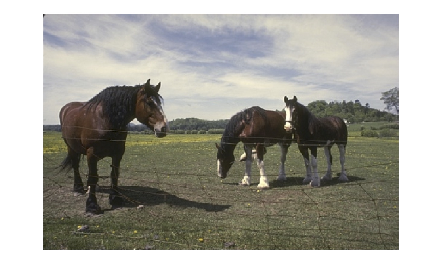
Original image	Ground truth	Level $s=1$	Level $s=2$
Level $s=3$	Level $s=4$	Level $s=5$	Level $s=6$

Figure 3: Example of classification with rejection (in black) across multiple levels in a natural image from the BSD500 data set.

We illustrate the robustness of the framework with regard to the number of scales by comparing the classification performance with a varying number of scales (Fig. 4). The variation of the number of scales is achieved by stacking coarser single-scale graphs on the multiscale graph, through an increase of the minimum superpixel size (MSS) by a factor of $2$: $1$ scale corresponds to a single scale graph of MSS $100$, $2$ scales to a multiscale graph of MSS of $(100,200)$, up to $11$ scales, that corresponds to a multiscale graph of MSS of $(100,200,\ldots,6400)$.

In Fig. 4 it is clear the performance improvement of using multiscale similarity graphs (more than one scale) against single scale similarity graphs (just one scale). The stabilization of the mean performance for more than $4$ scales is an indicator of the robustness of the framework with regard to the number of scales.

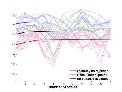
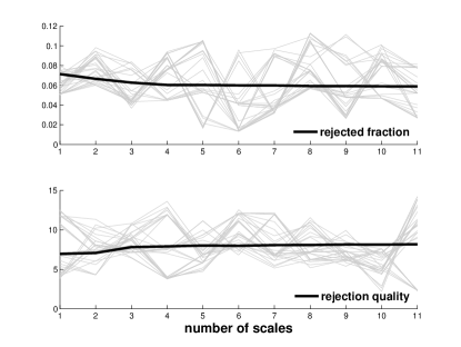
Figure 4: Evolution of classification performance with number of scales. Results obtained from $30$ Monte Carlo runs with different training sets of $10$ randomly selected samples per class of the image in Fig. 3. The variation of performance for more than $4$ scales is negligible.

VI-B H&E Data Set

Our H&E data set consists of 36 $1600\times 1200$-size images of H&E stained teratoma tissue slides imaged at $40\times$ magnification containing $20$ classes; Fig. 8 shows three examples.

VI-B1 Experimental Setup

As application-specific features we use the histopathology vocabulary (HV) [1, 4]. These features emulate the visual cues used by expert histopathologists [1, 2, 4], and are thus physiologically relevant. From the HV, we use nucleus size (1D), nucleus eccentricity (1D), nucleus density (1D), nucleus color (3D), red blood cell coverage (1D), and background color (3D). As similarity features we use the color on the RGB colorspace.

The statistic extracted for the application-specific and the similarity features, on the lowest level of the partition, consists of the sample mean of the feature values on the partition. It is a balance between good classification performance, low feature dimensionality, and low complexity. This results in $10$ dimensional application-specific feature vectors, and $3$ dimensional similarity feature vectors. The superclasses are constructed from the germ layer (endoderm, mesoderm, and ectoderm). Classes derived from the same germ layer will belong to the same superclass.

The multiscale similarity graph is built with six scales with a MSS of $(100,200,400,800,1600,3200)$ for each of the layers of the similarity graph. This provides a compromise between the computational burden associated with large similarity graphs and the performance increase obtained. The results we present with six scales are marginally better than the ones achieved with five or seven scales.

VI-B2 Parameter Analysis

In this section we analyze the impact of regularization parameter $\lambda$ on the LORSAL algorithm; the contextual index $\alpha$; and the rejection threshold $\rho$. The regularization parameter $\lambda$ describes the generalization capability of the classifier. The contextual index $\alpha$ describes the contextual information; $\alpha=0$ means no contextual information and $\alpha=1$ means no classification information is taken in account. The rejection threshold $\rho$ denotes our confidence in the classification result; lower values of $\rho$ denote low confidence in classification and higher values of $\rho$ denote high confidence in classification.

To evaluate the parameters, we define two types of training sets, based on the origin of the training samples: (1) A single image training set composed of $k$ samples $S_{k}$, extracted from a test image. This training set is used to train the classifier and is applied to the entire image. (2) A training set $S_{k,k}$ containing $k$ training samples from each image of a given set. This training set is used to evaluate the classifier in situations in which we have no knowledge about the tissues. Note that each of the $36$ H&E images not only contains a different set of tissues, but was also potentially stained and acquired using different experimental protocols, with no guarantee of normalization of the staining process.

The remaining parameters are set empirically according to the experts. The interscale ($v_{\textrm{interscale}}$) and intrascale ($v_{\textrm{intrascale}}$) weights for the similarity graph construction are set to $4$ and $1$, respectively, to achieve a “vertical” consistency in the multiscale classification. Larger values of the interscale when compared to the intrascale will enforce a higher multiscale effect on the segmentation: the different layers of the graph will be more similar to each other.

The superclass misclassification cost $g$ is set to $0.7$; the superclass consistency $\psi_{c}$ and rejection consistency $\psi_{r}$ are set to $0.7$ and $0.5$, respectively, to ease transitions into same superclass tissues and rejection, and to maintain a metric interaction potential. Larger values of the superclass consistency $\psi_{c}$ lead to smaller borders (in length) between elements of the same superclass, and smaller values lead to larger borders. The value of the rejection consistency $\psi_{r}$ affects the length of the border of the rejected areas (their perimeter): smaller values of $\psi_{r}$ lead to disconnected rejected areas (with a large perimeter), usually thin rejection zones between two different classes, whereas larger values of $\psi_{r}$ lead to connected rejected areas (with a small perimeter), usually rejection blobs that reject an entire area. To achieve similar levels of rejected fraction, the rejection threshold $\rho$ must accomodate the value of the $\psi_{r}$ as larger values of $\psi_{r}$ mean more costly rejection areas.

LORSAL Parameter Analysis

By varying the value of $\lambda$ in (6), we obtain different regressors ${\mathbf{W}}_{\lambda}$ (one matrix of parameters per value of $\lambda$. We expect that by increasing the value of $\lambda$ up to a point, a regressor with greater generalization capability can be obtained, thus with increased classification performance. However, increasing $\lambda$ furthermore will lead to lower performance, as the sparsity term in the optimization will overwhelm the data fit term. On the other hand, lower values of $\lambda$ will lead to an overfitted regressor, that will cause loss of performance.

To evaluate the generalization capability of the classifier, we test it with an entire data set training set $S_{75,75}$. With the entire data set training set created, each image is classified by the following maximum a posteriori classifier for each of the regressors $\hat{\mathbf{W}}_{\lambda}$ obtained for different values of $\lambda$:

$$\hat{y}_{i}=\arg\max_{\ell\in\mathcal{L}}p(y_{i}=\ell\mid\mathbf{f}_{i},{\mathbf{W}}_{\lambda})$$ (14)

The overall accuracy is computed for each image, as well as the sparsity of the regressor ${\mathbf{W}}_{\lambda}$.

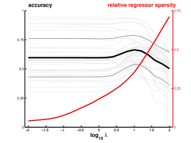
Figure 5: LORSAL parameter analysis. Effect of $\lambda$ on the overall accuracy values and sparsity of ${\mathbf{W}}$. Mean accuracy (in black), standard deviation (in gray), overlapped with the results for all images. Note the three zones of accuracy behavior: no effect, increase, decrease. The maximum overall accuracy ($66.4\%$) is obtained for $\lambda=10$ with a value of relative regressor sparsity of $0.352$.

From Figure 5, it is clear that there exist three different zones of accuracy behavior with the increasing sparsity of the regressor:

• For $0\leq\lambda\leq 1$ there is no effect — the data term vastly outweights the regularization term;

• For $1\leq\lambda\leq 10$ there is an increase in classification performance — increasing the regularization term will improve the generalization capability of the classifier;

• For $\lambda>10$ there is a decrease in classification performance — increasing the regularization term will hamper the capability of the classifier.

We empirically choose $\lambda$ to be $10$, as it maximizes the overall accuracy of the classifier.

Effect of contextual index, and rejection threshold in the classification performance

The inclusion of rejection in the classification leads to problems in the measurement of the performance of the classifier. As the accuracy is measured only on the nonrejected samples, it is not a good index of performance (the behavior of the classifier can be skewed to a very large reject fraction that will lead to nonrejected accuracies close to $1$). To cope with this, we use the quality of classification $Q$ [15]. The intuition being that, by maximizing $Q$, we maximize both the number of correctly classified samples not rejected and the number of incorrectly classified samples rejected.

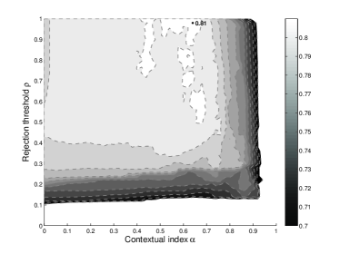
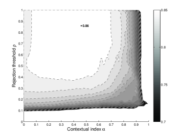
(a) $Q$ for $S_{60}$ (max. $Q$ $0.81$).	(b) $Q$ for $S_{120}$ (max. $Q$ $0.86$).
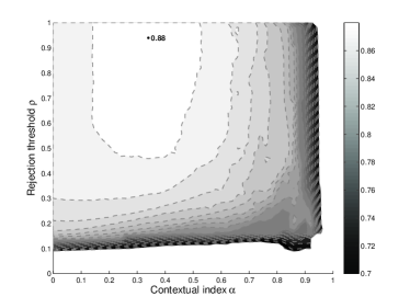
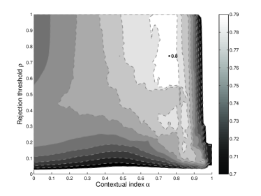
(c) $Q$ for $S_{240}$ (max. $Q$ $0.88$).	(d) $Q$ for $S_{60,60}$ (max. $Q$ $0.80$).

Figure 6: Variation of quality of classification $Q$ with the contextual index $\alpha$ and the rejection threshold $\rho$ for four different training sets. Adjacent contour lines correspond to a $0.01$ variation of $Q$. It is clear a shift to lower dependency on rejection and contextual information as the size of the training set, and consequently the classifier performance, increases.

By varying the value of the contextual index $\alpha$ in (12), we are weighting differently the role of contextual information in the classification. For $\alpha=0$, no contextual information is used, equivalent to (14), whereas for $\alpha=1$, the problem degenerates into assigning a single class to the entire image. By varying the value of the rejection threshold $\rho$ in (IV-A1), we are assigning different levels of confidence to the classifier, i.e., $\rho=0$ is equivalent to no confidence on the classifier (reject everything), whereas $\rho=1$ is equivalent to total confidence in the classifier (reject nothing).

As the contextual index $\alpha$ and the rejection threshold $\rho$ interact jointly, we now analyze the classification quality $Q$ for different situations.

We test with three single image training sets $S_{60}$, $S_{120}$, $S_{240}$, corresponding roughly to using $1.5\%$, $3\%$ and $6\%$ of the samples of the image. We test with an entire data set training set $S_{60,60}$, on which only $3\%$ of the data set is composed of samples from the test image. For each type of training set, we use as test images each of the $36$ images of the data set, presenting the mean value of $Q$.

From Figure 6, we can observe the variation of the performance of the classifier with $\alpha$ and $\rho$ for different situations. The change from (a) to (c) corresponds to an increase in the dimension of the training set. Both the improvement of the maximum value and the shift to lower values of contextual index and higher values of rejection threshold can be explained by increasing performance of the classification. This means that a more reliable classification is available, decreasing the need to use contextual information and rejection. On the other hand, (d) corresponds to an extreme situation in which the training set is highly noisy, with only $3\%$ of samples belonging to the test image. The high dependency of contextual information in this case is clear. The maximum value of $Q$ is attained at lower values of the rejection threshold and higher values of the contextual index.

VI-B3 Parameter Selection

As seen in Figure 6, the quality of classification varies with the type of applications; applications for which the training set is easier will lead to lower reliance on contextual information and rejection, and harder training sets will lead to the opposite. In order to select a single set of parameters, we combine the results of the four different training sets for each of the $36$ images, obtaining the average of the classification quality $Q$ and nonrejected accuracy for the resulting $4\times 36$ instances. Our motivation for the selection of the parameters is to maximize the accuracy of the nonrejected fractions within a zone of high classification quality. To do so, we select the region of high values of $Q$ ($Q$ higher than $99\%$ of its maximum value). Then we select the parameters that maximize the nonrejected accuracy, as seen in Figure 7.

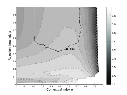
Figure 7: Variation of nonrejected accuracy with the contextual index $\alpha$ and rejection threshold $\rho$. The dark line corresponds to the level set of quality of classification $Q$ equal to $99\%$ of its maximum value. The maximum nonrejected accuracy is $85\%$, corresponding to $\rho=0.46$ and $\alpha=0.58$. The corresponding rejection fraction $r$ is $4.6\%$.

TABLE I: Classification and rejection performance metrics for the example images in Figure 8. Classification with rejection and context (white background), classification with context without rejection (green background), classification without context with rejection (red background), and classification without context and without rejection (brown background).

Image	Nonrejected accuracy	Rejected fraction	Rejectio quality	Classification quality	Accuracy with no rejection
Classification with rejection and context
$1$	${0.701}$	$0.347$	$3.37$	$0.662$	${0.600}$
$2$	$0.891$	$0.067$	$10.11$	$0.868$	$0.862$
$3$	$0.967$	$0.140$	$9.97$	$0.866$	$0.937$
Classification with rejection without context
$1$	$0.702$	$0.370$	$3.90$	$0.673$	$0.582$
$2$	$0.878$	$0.031$	$9.69$	$0.868$	$0.863$
$3$	$0.936$	$0.000$	$3920$	$0.936$	$0.935$

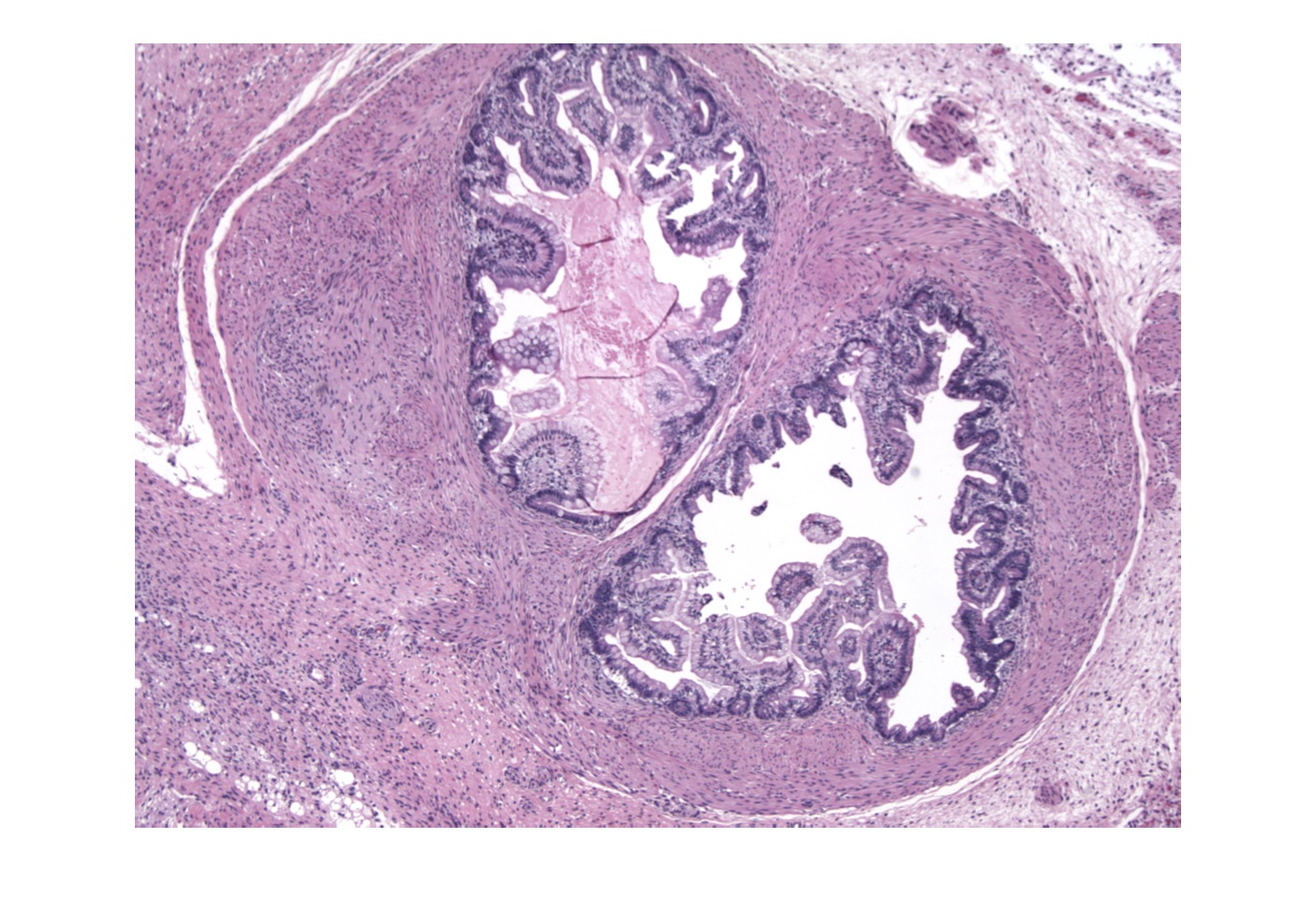
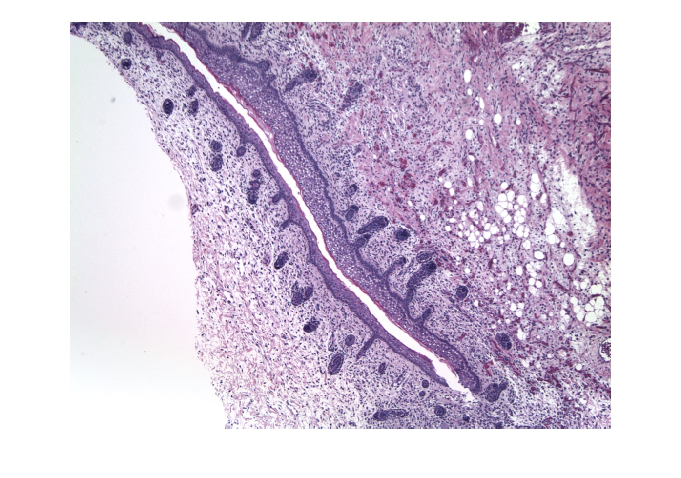
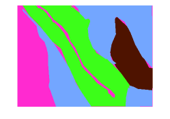
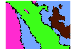
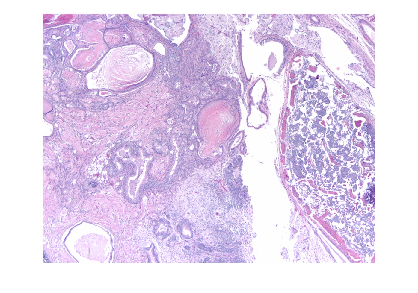
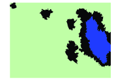
(a) Original image.	(b) Ground truth.	(c) Classification result.

Figure 8: Example of classification results for H&E stained samples of teratoma imaged at $40X$ containing multiple tissues: Image 1 (first row) background (light pink), smooth muscle (dark pink), gastro intestinal (purple), mature neuroglial (light brown), fat (dark brown); mesenchyme (light blue); Image 2 (second row) background (light pink), fat (dark brown), mesenchyme (light blue), skin (green); Image 3 (third row) mesenchyme (light green); bone (dark blue). Rejected partitions are shown in black. The training set consists of: $5$ randomly chosen partitions per class (roughly $0.6\%$ of total) for image 1, $120$ randomly chosen partitions (roughly $3\%$ of total) for image 2, $20$ randomly chosen partitions (roughly $0.5\%$ of total) for image 3; with the $\lambda$ parameter set to $5$.

TABLE II: Class-specific results for the example images in Figure 8.

Tissue	Train	Test	Rejected	Rejection	Nonrejected	Classification	Accuracy
type	samples	samples	samples	quality	accuracy	quality	no rejection
Image 1
Other	$5$	$410$	$134$	$0.77$	$0.72$	$0.55$	$0.75$
Fat	$5$	$54$	$1$	$0.00$	$0.94$	$0.93$	$0.93$
Gastrointestinal	$5$	$1036$	$170$	$3.90$	$0.91$	$0.83$	$0.86$
Smooth muscle	$5$	$1283$	$529$	$1.81$	$0.69$	$0.64$	$0.58$
Mesenchyme	$5$	$454$	$174$	$4.04$	$0.53$	$0.66$	$0.38$
Mat. neuroglial	$5$	$369$	$143$	$1.82$	$0.35$	$0.53$	$0.29$
Image 2
Other	$30$	$885$	$24$	$5.80$	$0.91$	$0.90$	$0.90$
Fat	$13$	$510$	$48$	$4.54$	$0.77$	$0.75$	$0.74$
Skin	$36$	$1157$	$37$	$20.35$	$0.98$	$0.96$	$0.97$
Mesenchyme	$41$	$1268$	$127$	$6.17$	$0.86$	$0.83$	$0.82$
Image 3
Bone	$2$	$725$	$246$	$1.60$	$0.75$	$0.64$	$0.69$
Mesenchyme	$18$	$3195$	$319$	$11.27$	$1.00$	$0.91$	$0.99$

VI-B4 Results

We present results of our method on a set of $3$ images from the data set containing a different number of classes (as seen in Figure 8). The classifications are obtained with different training sets to illustrate different challenges. In image $1$, to create a small and nonrepresentative training set, the training set is composed of $5$ randomly chosen partition elements per class (roughly $0.6\%$ of total). In image $2$, to create a representative training set, the training set is composed of $120$ randomly chosen partition elements from the entire image (roughly $3\%$ of total). In image $3$, to create a small representative training set with high class overlap, the training set is composed of $20$ randomly chosen partition elements from the entire image (roughly $0.5\%$ of total). In all cases, the $\lambda$ parameter is set to $5$, with the rest of the parameters unchanged.

We analyze both overall results (in Table I) and class-specific results (in Table II). The computation of the rejection quality is based on the results of classification with contextual information and no rejection (i.e. comparing the labeling with rejection to the labeling resulting from setting the reject threshold $\rho$ to $1$ in (12)).

In Table I, we compare the performance of classification with contextual information and rejection with context only (obtained by setting $\rho=1$) and with classification with rejection only with optimal rejected fraction (obtained by sorting the partition elements according to maximum a posterior probability and selecting the rejected fraction that maximizes the classification quality).

Comparing the performance results of classification with rejection using contextual information (white background in Tab. I) with the results of classification with context only (red background in Tab. I), the improvement in classification accuracy at the expense of introducing rejection is clear. For images $1$ and $2$, this can be achieved at levels of classification quality higher than accuracy of context only, meaning that we are rejecting misclassified samples at a proportion that increases the number of correct decisions made (the underlying concept of classification quality). For image $3$, due to the high accuracy of context only (and of the classification with no context and no rejection, brown background in Tab. I), the increase in accuracy is at the expense of rejecting a comparatively large proportion of correctly classified samples, leading to a smaller value of classification quality.

Comparing the performance results of classification with rejection using contextual information with the results of classification with rejection only with optimal rejected fraction (red background in Tab. I) the results are comparable for images $1$ and $2$, meaning we can achieve a performance improvement similar to the achieved by rejection with optimal rejected fraction through the introduction of context. For image $3$, due to the high accuracy of classification with no context and no rejection (brown background in Tab. I), the optimal rejected fraction is $0$, meaning that the increased accuracy is at the expense of rejecting a comparatively large proportion of correctly classified samples.

Analyzing the classification in Fig. 8, the effects of combining rejection with contextual information are clear. We obtain significant improvements for image $1$ by combining classification with context with classification with rejection in terms of classification quality and nonrejected accuracy, thus revealing the potential of combining classification with rejection with classification with context. For image $2$, only the class boundaries are rejected, leading to high values of overall rejection quality and class-specific rejection quality. In image $3$, it is clear the effect of noisy training sets (due to the image characteristics), where a significant amount of the class boundaries are rejected, and the classification quality is lower than the accuracy of the original classification with no context and no rejection.

Finally, we point to the usefulness of the classification quality $Q$. By analysis of the classification quality, it is possible to compare the performance of the classifier with rejection in different situations and note how the performance will decrease as the complexity of the problem increases (by increasing the number of classes).

VII Conclusions

We proposed a classifier where by combining classification with rejection with classification using contextual information we are able to increase classification accuracy. Furthermore, we are able to impose spatial constraints on the rejection itself departing from the current standard of image classification with rejection. These encouraging results point towards potential application of this method in large-scale automated tissue identification systems of histological slices as well as other classification tasks.

References

- [1] R. Bhagavatula, M. C. Fickus, J. W. Kelly, C. Guo, J. A. Ozolek, C. A. Castro, and J. Kovačević, “Automatic identification and delineation of germ layer components in H&E stained images of teratomas derived from human and nonhuman primate embryonic stem cells,” in Proc. IEEE Int. Symp. Biomed. Imag., Rotterdam, Apr. 2010, pp. 1041–1044.
- [2] M. T. McCann, R. Bhagavatula, M. C. Fickus, J. A. Ozolek, and J. Kovačević, “Automated colitis detection from endoscopic biopsies as a tissue screening tool in diagnostic pathology,” in Proc. IEEE Int. Conf. Image Process., Orlando, FL, Sept. 2012, pp. 2809–2812.
- [3] F. Condessa, J. Bioucas-Dias, C. A. Castro, J. A. Ozolek, and J. Kovačević, “Classification with rejection option using contextual information,” in Proc. IEEE Int. Symp. Biomed. Imag., San Francisco, CA, Apr. 2013, pp. 1340–1343.
- [4] R. Bhagavatula, M. T. McCann, M. C. Fickus, C. A. Castro, J. A. Ozolek, and J. Kovačević, “A vocabulary for the identification of teratoma tissue in H&E-stained samples,” J. Pathol. Inform., vol. 5, no. 19, June 2014.
- [5] C. K. Chow, “On optimum recognition error and reject tradeoff,” IEEE Trans. Inf. Theory, vol. 16, no. 1, pp. 41–46, Jan. 1970.
- [6] G. Fumera, F. Roli, and G. Giacinto, “Reject option with multiple thresholds,” Patt. Recogn., vol. 33, no. 12, pp. 2099–2101, Dec. 2000.
- [7] R. Herbei and M. Wegkamp, “Classification with reject option,” Canadian Journal of Statistics, vol. 34, no. 4, pp. 709–721, 2006.
- [8] P. Foggia, C. Sansone, F. Tortella, and M. Vento, “Multiclassification; reject criteria for the bayesian combiner,” Patt. Recogn., vol. 32, no. 8, pp. 1435–1447, Aug. 1999.
- [9] G. Fumera and F. Roli, “Support vector machines with embedded reject option,” in Proc. Int. Workshop on Pattern Recognition with Support Vector Machines (SVM2002), Niagara Falls, Niagara Falls, Canada, Aug. 2002, pp. 68–82, Springer-Verlag.
- [10] P. Bartlett and M. Wegkamp, “Classification methods with reject option using a hinge loss,” Journal Machine Learning Research, vol. 9, pp. 1823–1840, Aug. 2008.
- [11] M. Yuan and M. Wegkamp, “Classification methods with reject option based on convex risk minimization,” Journal Machine Learning Research, vol. 11, pp. 111–130, Mar. 2010.
- [12] M. Wegkamp, “Lasso type classifiers with a reject option,” Electronic Journal of Statistics, pp. 155–168, 2007.
- [13] P. Foggia, G. Percannella, C. Sansone, and M. Vento, “On rejecting unreliably classified patterns,” in Multiple Classifier Systems, M .Haindl, J. Kittler, and F. Roli, Eds., vol. 4472 of Lecture Notes in Computer Science, pp. 282–291. Springer, 2007.
- [14] I. Pillai, G. Fumera, and F. Roli, “Multi-label classification with a reject option,” Patt. Recogn., vol. 46, no. 8, pp. 2256 – 2266, 2013.
- [15] F. Condessa, J. Bioucas-Dias, and J. Kovačević, “Performance measures for classification systems with rejection,” Preprint, 2015, arxiv.org/abs/1504.02763 [cs.CV].
- [16] Y. Boykov, O. Veksler, and R. Zabih, “Fast approximate energy minimization via graph cuts,” IEEE Trans. Pattern Anal. Mach. Intell., vol. 20, no. 11, pp. 1222–1239, Nov. 2001.
- [17] S. Kumar and M. Hebert, “Discriminative random fields,” Int. J. Comput. Vis., vol. 68, no. 2, pp. 179–201, 2006.
- [18] J. Li, J. Bioucas-Dias, and A. Plaza, “Hyperspectral image segmentation using a new bayesian approach with active learning,” IEEE Trans. Geosci. Remote Sens., vol. 49, no. 10, pp. 3947–3960, Oct. 2011.
- [19] J .Bioucas-Dias, A. Plaza, G. Camps-Valls, P. Scheunders, N. Nasrabadi, and J. Chanussot, “Hyperspectral remote sensing data analysis and future challenges,” Geoscience and Remote Sensing Magazine, IEEE, vol. 1, no. 2, 2013.
- [20] S. Li, Markov Random Field Modeling in Image Analysis, Springer-Verlag, 2nd edition, 2001.
- [21] D. Böhning, “Multinomial logistic regression algorithm,” Ann. Inst. Stat. Math., vol. 44, no. 1, pp. 197–200, Mar. 1992.
- [22] B. Krishnapuram, L. Carin, M. Figueiredo, and A. Hartemink, “Sparse multinomial logistic regression: Fast algorithms and generalization bounds,” IEEE Trans. Pattern Anal. Mach. Intell., vol. 27, no. 6, pp. 957 – 967, June 2005.
- [23] D. Bertsekas J. Eckstein, “On the Douglas–Rachford splitting method and the proximal point algorithm for maximal monotone operators,” Mathematical Programming, vol. 55, no. 1-3, pp. 293–318, 1992.
- [24] V. Kolmogorov and R. Zabih, “What energy functions can be minimized via graph cuts?,” IEEE Trans. Pattern Anal. Mach. Intell., vol. 26, no. 2, pp. 147–159, Feb. 2004.
- [25] Y. Boykov and V. Kolmogorov, “An experimental comparison of min-cut/max-flow algorithms for energy minimization in vision,” IEEE Trans. Pattern Anal. Mach. Intell., vol. 26, no. 9, pp. 1124–1137, Sept. 2004.
- [26] P. F. Felzenszwalb and D. P. Huttenlocher, “Efficient graph-based image segmentation,” Int. J. Comput. Vis., vol. 59, no. 2, pp. 167–181, 2004.
- [27] D. Martin, C. Fowlkes, D. Tal, and J. Malik, “A database of human segmented natural images and its application to evaluating segmentation algorithms and measuring ecological statistics,” in Proc. 8th Int’l Conf. Computer Vision, July 2001, vol. 2, pp. 416–423.
- [28] F. Condessa, J. Bioucas-Dias, C. Castro, J. Ozolek, and J. Kovačević, “Image classification with rejection using contextual information,” available at http://jelena.ece.cmu.edu/repository/rr/15_CondessaBCOK/15_CondessaBCOK.html.