Inca Foams

Abstract.

We study a certain class of embedded two-foams that arise from gluing discs into ribbon torus knots along nonintersecting torus meridians. We exhibit several equivalent diagrammatic formalisms for these objects and identify several of their invariants, including a unique prime decomposition.

1. Introduction

An embedded $2$–foam in standard Euclidean $\mathds{R}^{4}$ is a $2$–dimensional analogue of a knotted trivalent graph $\mathds{R}^{3}$. We investigate a certain class of embedded $2$–foams which we call Inca foams (this name was suggested to us from [23]) that arise from gluing discs into ribbon torus knots along nonintersecting torus meridians. We exhibit five diagrammatic formalisms for Inca foams. We then identify several invariants of Inca foams, including their unique prime decompositions.

The geometric topological study of embedded $2$–foams was initiated by Carter [8]. A knotted surface in $\mathds{R}^{4}$ is in particular a $2$–foam, and so the theory of embedded $2$–foams is at least as complicated the theory of knotted surfaces in dimension $4$ [9]. Inca foams are a much simpler class of objects than $2$–foams (e.g. no local knotting) but are still complicated enough to be interesting. The theory of coloured versions of such foams is equivalent to a construction that was used by the authors to topologically model fusion of information and as a model for computation [4, 5, 7], and it is this that is our main motivation.

We describe the contents of this paper. Section 2 defines Inca foams which Section 3 describes in five (5) different diagrammatic ways. The first is a broken surface diagram of the foam, the second is a broken surface diagram of tangled spheres and intervals, the third is a $3$–dimensional analogue of a tangle diagram, the fourth is a tangle diagram, and the fifth is a Gauß diagram. Section 4 proves that these are equivalent. Each of the diagrammatic formalisms is useful for something else. The more topological ones are better for proving theorems, and the more combinatorial ones are better for defining invariants.

Section 5 describes some simple Inca foam invariants. Some, such as underlying graph and underlying w-tangle, are structures which we obtain by suppressing some of the information in an Inca foam. Some, such as the fundamental quandle and the linking graph, are analogues of classical link invariants. One, the Shannon capacity, is an analogue of a graph invariant.

Section 6 discusses unique prime decomposition for connected Inca foams. The prime decomposition is of course an invariant up to permutation of factors. Existence and uniqueness of prime decomposition indicates how well-behaved this class of objects is in comparison with classes such as virtual tangles and w-tangles.

Much of the content of this paper originally appeared in the preprint [6], which is being split into parts, the first of which is the present paper.

2. Inca foams

So what is an Inca foam? We give the definition below.

Definition 2.1.

Parameterize $S^{1}\simeq\mathds{R}/\mathds{Z}$, and for a given $k\geq 1$, glue $2$–discs $D_{1},\ldots,D_{k}$ to a torus $T^{2}\stackrel{{\scriptstyle\textup{\tiny def}}}{{=}}S^{1}\times S^{1}$ so that $\partial D_{j}$ glues to $S^{1}\times\left\{\frac{j}{k}\right\}$ for $j=1,2,\ldots,k$. Call the resulting shape $K_{k}$. An Inca foam is an immersion

$$F\colon\,\bigcup_{i=1}^{\nu}K_{k_{i}}\to S^{4}\simeq\mathds{R}^{4}\cup\left\{\infty\right\}\enspace,$$

whose restriction to $\mathds{R}^{4}$ is an embedding, for which $F(T^{2})$ bounds a solid torus for each $K_{k_{i}}$. In the above, $k_{1},k_{2},\ldots,k_{\mu}$ are positive integers. Call $F(K_{k_{1}}),F(K_{k_{2}}),\ldots,F(K_{k_{\nu}})$ the components of $F$. See Figure 1.

Equivalently (and to fix notation), $F(D_{i}\cup(S^{1}\times[\frac{i}{n},\frac{i+1}{n}])\cup D_{i+1})$ is homeomorphic to a sphere $S_{i}$, and this sphere must bound a $3$–ball $B_{i}$ in $S^{4}$.

We additionally require that the special point $\left\{\infty\right\}\in S^{4}$ lie either outside the bounded solid tori, or else that it lie in the interior of at most one of the $2$–discs for each connected component. Thus, different connected components might intersect but only inside their $2$–discs and only at the point $\infty$.

Figure 1. A Roseman, a Rosemeister, and a Reidemeister diagram of an Inca foam.

Our convention is that our objects live in the smooth category, and we smooth corners automatically at every step usually without comment. Such sloppiness is standard in geometric topology— [17] famously begins with the words “…the phrase “corners can be smoothed” has been a phrase that I have heard for 30 years, and this is not the place to explain it”.

Various generalizations of Definition 2.1 suggest themselves. For example, if we allow each sphere to intersect an arbitrary number of other spheres at disjoint disks, i.e. if we consider surfaces of higher genus than tori, then the effect is only to make diagrams and notations more complicated— the mathematics is essentially unchanged and all of our constructions generalize in a straightforward way. For example, the underlying graph of a Gauß diagram (see Section 3.5) becomes an arbitrary graph instead of a collection of paths and cycles. If disks are allowed to have disk intersection then trees replace intervals e.g. in Section 3.2, and underlying graphs have two different kinds of vertices; Everything generalizes to this setting as well but more work is needed.

Inca foams are considered equivalent if they are ambient isotopic in $\mathds{R}^{4}$, a definition which we recall below in our setting:

Definition 2.2 (Ambient isotopy).

Consider a class $\mathfrak{T}$ of embedded objects in standard $S^{4}\simeq\mathds{R}^{4}\cup\{\infty\}$. Two embedded objects $T_{1},T_{2}\in\mathfrak{T}$ are ambient isotopic in $\mathds{R}^{4}$ if there exists a smooth homeomorphism $h\colon\,\mathds{R}^{4}\times[0,1]\to\mathds{R}^{4}$ with $h(T_{1}\times\{0\})=T_{1}$, and $h(T_{1}\times\{t\})$ is an element of $\mathfrak{T}$ for all $t\in[0,1]$, and $h(T_{1}\times\{1\})=T_{2}$.

We further define (de)stabilization to be the following operation.

Definition 2.3 (Stabilization; Destabilization).

Let $S$ be a sphere in an Inca foam $F$ which bounds a ball $B$ whose interior does not intersect $F$. Let $S^{\prime}$ be a sphere in $F$ which shares a disk $D$ with $S$. The destabilization of $F$ by $D$ is the Inca foam obtained by erasing $D$ from $F$ and smoothing corners (so that $S$ and $S^{\prime}$ effectively become a single sphere). The inverse operation to destabilization is called stabilization. See Figure 2.

$\begin{minipage}{28.45274pt}\includegraphics[height=85.35826pt]{foam_stabilize2}\end{minipage}\quad\longleftrightarrow\quad\begin{minipage}{28.45274pt}\includegraphics[height=85.35826pt]{foam_stabilize1}\end{minipage}$

Figure 2. Stabilization of Inca foams.

Definition 2.4 (Equivalence; Stable equivalence).

Two Inca foams are said to be equivalent if they are ambient isotopic. They are said to be stably equivalent if they have equivalent stabilizations.

3. Five diagrammatic descriptions

This section describes Inca foams in five different ways, starting from the most geometric and progressing to the most combinatorial. Section 4 proves that these describe the same objects. The more geometric descriptions are easier to use to prove theorems with, while the more combinatorial ones are better suited for calculations.

Formalism	Section	Agent	Local moves	Stabilization
Inca foams	3.1		Carter–Roseman moves [8].	$\quad\begin{minipage}{11.38092pt}\includegraphics[height=34.14322pt]{foam_stabilize2}\end{minipage}\longleftrightarrow\begin{minipage}{11.38092pt}\includegraphics[height=34.14322pt]{foam_stabilize1}\end{minipage}\quad$
Roseman	3.2			$\begin{minipage}{11.38092pt}\ \,\includegraphics[height=34.14322pt]{vline}\end{minipage}\rule{0.0pt}{51.21504pt}\longleftrightarrow\ \begin{minipage}{11.38092pt}\includegraphics[height=39.83368pt]{si_agent}\end{minipage}$
Rosemeister	3.3		\psfrag{r}[c]{}\psfrag{s}[c]{}\psfrag{t}[c]{}\psfrag{u}[c]{}\includegraphics[width=411.93767pt]{moves_4d2a.eps}	$\begin{minipage}{11.38092pt}\ \,\includegraphics[height=34.14322pt]{vline}\end{minipage}\longleftrightarrow\ \begin{minipage}{11.38092pt}\includegraphics[height=39.83368pt]{rosemeister_agent}\end{minipage}$
Reidemeister	3.4			$\begin{minipage}{11.38092pt}\ \,\includegraphics[height=34.14322pt]{vline}\end{minipage}\longleftrightarrow\ \begin{minipage}{11.38092pt}\includegraphics[height=34.14322pt]{Reidemeister_agent}\end{minipage}$
Gauß diagram,	3.5

Table 1. The five diagrammatic formalisms for Inca foams.

3.1. Roseman diagrams of foams

Any embedded surface $F$ in $\mathds{R}^{4}$ can be drawn in $\mathds{R}^{3}$ by projecting $F$ onto a choice of $3$–plane $H\subset\mathds{R}^{4}$. We choose a generic projection so that neighbourhoods of singular points are as shown in Figure 3. Break the surface to keep track of ‘under’ and ‘over’ information. The resulting diagram is called a broken surface diagram [9].

Figure 3. Neighbourhoods of singular points of a generic $3$–dimensional projection of a knotted surface in $\mathds{R}^{4}$.

Roseman’s Theorem for Foams provides a collection of $15$ local moves on broken surface diagrams so that any two $2$–foams are ambient isotopic if and only if any broken surface diagram of one is related to any broken surface diagram of the other by a finite sequence of these Carter–Roseman moves [14, 10, 20, 8].

Two Roseman diagrams are (stably) equivalent if a pair of $2$–foams which they represent are (stably) equivalent.

3.2. Roseman diagrams of sphere and interval tangles

Our next diagrammatic formalism allows us to ignore the Carter–Roseman moves which we do not need in our context because our disks are disjoint and our spheres have no local knotting. By convention, when we say Roseman diagram without further specification, what we meet is a Roseman diagram of a sphere and interval tangle as defined in this section.

Definition 3.1 (Sphere and Interval Tangle).

A connected sphere and interval tangle is a union

$$L\stackrel{{\scriptstyle\textup{\tiny def}}}{{=}}L_{1}\sqcup L_{2}\sqcup\cdots\sqcup L_{\nu},$$

of disjointly embedded objects in standard Euclidean $\mathds{R}^{4}$ defined as follows:

• A set $S_{1},S_{2},\ldots,S_{k}$ of $2$–spheres embedded in $\mathds{R}^{4}$ such that there exist disjointly embedded closed $2$–balls $B_{1},B_{2},\ldots B_{k}$ with $\partial B_{j}=S_{j}$ for $j=1,2,\ldots k$.

• Identifying $S^{4}\simeq\mathds{R}^{4}\cup\left\{\infty\right\}$, a set of closed intervals $I_{1},I_{2},\ldots,I_{m}$ disjointly embedded in $S^{4}$ such that each interval endpoint lies on a sphere. We allow no other intersections between intervals and spheres. Write $L_{i}\stackrel{{\scriptstyle\textup{\tiny def}}}{{=}}\bigcup_{j=1}^{k}I_{j}\cup S_{j}$. Only $I_{m}$ may pass through the point $\infty$, and if it does then we call $L_{i}$ open (because $I_{m}$ splits into two rays when we restrict to $\mathds{R}^{4}$) otherwise we call it closed.

A sphere and interval tangle is a union of connected sphere and interval tangles which may intersect one another only at the point $\infty$.

Stabilization of a sphere and interval tangle is:

(1) $$\begin{minipage}{17.07182pt}\ \,\includegraphics[height=51.21504pt]{vline}\end{minipage}\longleftrightarrow\quad\begin{minipage}{17.07182pt}\includegraphics[height=56.9055pt]{si_agent}\end{minipage}$$

Sphere and interval tangles also admit Roseman diagrams. Their equivalence is defined as follows.

Definition 3.2 (Equivalence of Roseman diagrams of sphere and interval tangles).

Two Roseman diagrams of sphere and interval tangles are equivalent if they are related by a finite sequence of the local moves of Figure 4. They are stably equivalence if they are related by a finite sequence of these moves and (de)stabilizations.

Figure 4. Local moves on Roseman diagrams of sphere and interval tangles.

3.3. Rosemeister diagrams

The interior of the sphere in a Roseman diagram of a sphere and interval tangle plays no role except to confuse. If spheres of Roseman diagrams do not intersect, then we may crush the sphere to a disk without loss of information. One advantage of eliminating redundant sphere interiors is that intervals of Rosemeister diagrams can be coloured, with colours changing as they pass through disks- see Section 5.3.

Stabilization of a Rosemeister diagram is

(2) $$\begin{minipage}{17.07182pt}\ \,\includegraphics[height=51.21504pt]{vline}\end{minipage}\longleftrightarrow\quad\begin{minipage}{17.07182pt}\includegraphics[height=56.9055pt]{rosemeister_agent}\end{minipage}$$

Definition 3.3 (Equivalence of Rosemeister diagrams).

Two Rosemeister diagrams are equivalent if they are related by a finite sequence of the local moves of Figure 5. They are stably equivalence if they are related by a finite sequence of these moves and (de)stabilizations.

\psfrag{r}[c]{\small\emph{R1}}\psfrag{s}[c]{\small\emph{R2}}\psfrag{t}[c]{\small\emph{R3}}\psfrag{u}[c]{\small\emph{VR}}\includegraphics[width=411.93767pt]{moves_4d2a.eps}

Figure 5. Local moves on Rosemeister diagrams of sphere-and-interval tangles.

3.4. Reidemeister diagrams

A Reidemeister diagram of a sphere and interval tangle $T$ is a generic projection of $T$ onto a $2$–plane for which images of spheres are disjoint and are designated by thick lines. The authors find this the simplest diagrammatic formalism with which to visualize objects. Stabilization is defined as follows:

(3) $$\begin{minipage}{28.45274pt}\ \,\includegraphics[height=85.35826pt]{vline}\end{minipage}\ \longleftrightarrow\qquad\begin{minipage}{28.45274pt}\includegraphics[height=85.35826pt]{Reidemeister_agent}\end{minipage}$$

Definition 3.4 (Equivalence of Rosemeister diagrams).

Two Reidemeister diagrams are equivalent if they are related by a finite sequence of the local moves of Figure 6, called cosmetic moves and Figure 7, called Reidemeister moves. They are stably equivalence if they are related by a finite sequence of these moves and (de)stabilizations.

\psfrag{a}[c]{$\triangleright$}\psfrag{b}[c]{$\triangleleft\,$}\psfrag{V}[c]{\small\emph{I1}}\psfrag{x}[c]{$x$}\psfrag{T}[c]{\small\emph{VR1}}\psfrag{R}[c]{\small\emph{VR2}}\psfrag{S}[c]{\small\emph{VR3}}\psfrag{Q}[c]{\small\emph{SV}}\psfrag{D}[c]{\small\emph{I2}}\psfrag{E}[c]{\small\emph{FM1}}\psfrag{F}[c]{\small\emph{FM2}}\psfrag{C}[c]{\small\emph{I3}}\psfrag{Y}[c]{\small\emph{ST}}\psfrag{X}[c]{\small\emph{ST}}\includegraphics[width=368.57964pt]{VR2}

Figure 6. Cosmetic moves for Reidemeister diagrams. Directions are not indicated, which means that the moves are valid for all directions so long as the directions on the RHS and on the LHS match up.

\psfrag{T}[c]{\small\emph{VR1}}\psfrag{R}[c]{\small\emph{VR2}}\psfrag{S}[c]{\small\emph{VR3}}\psfrag{Q}[c]{\small\emph{SV}}\psfrag{D}[c]{\small\emph{R1}}\psfrag{A}[c]{\small\emph{R2}}\psfrag{B}[c]{\small\emph{R3}}\psfrag{C}[c]{\small\emph{UC}}\psfrag{X}[c]{\small\emph{ST}}\includegraphics[width=368.57964pt]{R_moves1}

Figure 7. Reidemeister moves for Reidemeister diagrams, valid for any directions of the thick lines (directions on the LHS and on the RHS must match up).

3.5. Gauß Diagrams

Our final diagrammatic formalism is combinatorial and is based on labeled graphs. It is minimal and as such it’s the simplest to use for defining some invariants.

Definition 3.5 (Gauß diagram of an Inca foam).

A Gauß diagram of an Inca foam is a triple $M\stackrel{{\scriptstyle\textup{\tiny def}}}{{=}}(G,S,\phi)$ consisting of:

• A finite graph $G$ that is a disjoint union of path graphs $P_{1},\ldots,P_{k}$ and cycles $C_{1},\ldots,C_{l}$:

  (4) $$G\,\stackrel{{\scriptstyle\textup{\tiny def}}}{{=}}\,\left(P_{1}\,\raisebox{1.25pt}{\scalebox{0.8}{$\coprod$}}\;P_{2}\,\raisebox{1.25pt}{\scalebox{0.8}{$\coprod$}}\;\cdots\,\raisebox{1.25pt}{\scalebox{0.8}{$\coprod$}}\;P_{k}\right)\,\raisebox{1.25pt}{\scalebox{0.8}{$\coprod$}}\;\left(C_{1}\,\raisebox{1.25pt}{\scalebox{0.8}{$\coprod$}}\;C_{2}\,\raisebox{1.25pt}{\scalebox{0.8}{$\coprod$}}\;\cdots\,\raisebox{1.25pt}{\scalebox{0.8}{$\coprod$}}\;C_{l}\right),$$

  The graph $G$ is called the underlying graph of $M$.

• A subset of registers $S\subseteq V(G)$ called agents.

• A multivalued interaction function $\phi\colon\,S\Rightarrow E(G)\times\left\{\leftarrow,\rightarrow\right\}$ specifying the edges acted on by each agent and a direction $\leftarrow$ or $\rightarrow$.

Two Gauß diagrams $M_{1}$ and $M_{2}$ are considered equivalent if they are related by a finite sequence of the following Reidemeister moves:

Reidemeister I

Here, directions of edges $\leftarrow$ or $\rightarrow$ are arbitrary:

(5)

Reidemeister II

In following local modification, the top central vertex must be outside the set of agents $S$.

(6)

Reidemeister III

All edges in $\phi(e)$ in the expression below must participate in the move (the move is invalid for a strict subset of them). Directions $\leftarrow$ or $\rightarrow$ are arbitrary but should correspond on the left and right as indicated in the example below:

(7)

The following move is called stabilization, where one of the registers on the LHS must lie outside the image of $\phi$:

(8)

By convention, the stabilization of a single vertex is a $2$–vertex line graph.

Definition 3.6 (Equivalence of Gauß diagrams).

Two Gauß diagrams are equivalent if they are related by a finite sequence of Reidemeister moves. They are stably equivalence if they are related by a finite sequence of these moves and (de)stabilizations.

4. Proof of equivalence

The goal of this section is the following theorem:

Theorem 4.1.

Stable equivalence classes of all of the diagrammatic formalisms in Section 3 are in bijective correspondence with stable equivalence classes of Inca foams.

Proof.

$\text{Gau{\ss} }\Leftrightarrow\text{ Reidemeister}$:

This equivalence was proven in [5]. To obtain a Reidemeister diagram from a Gauß diagram, first destabilize until each edge is in the $\phi$–image of some agent. Then replace interactions as follows:

(9)

The indeterminacy in the translation from Gauß diagram interactions to tangle diagram interactions is captured by moves $I1$, $I2$ and $I3$ in Figure 6.

Then concatenate as dictated by the graph, as in Figure 8. The indeterminacy in doing this is captured by moves $V\!R1$, $V\!R2$, $V\!R3$, and $SV$ in Figure 6. Once tangle endpoints have been ‘sent to infinity’, there are no further indeterminacies.

Reidemeister moves on Gauß diagrams correspond to Reidemeister moves on Reidemeister diagrams by construction.

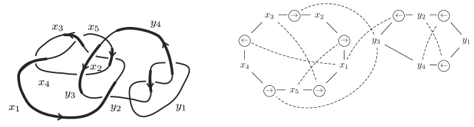
Figure 8. A Gauß diagram and corresponding Reidemeister diagram.

$\text{Reidemeister }\Leftrightarrow\text{ Rosemeister}$:

Begin by constructing a local model for a single interaction, consisting of a single over-strand $A$ with $k$ strands passing up through it and $l$ strands passing down through it. Consider a $2$–disc in Euclidean $\mathds{R}^{4}$:

(10) $$D\stackrel{{\scriptstyle\textup{\tiny def}}}{{=}}\left\{\left.\rule{0.0pt}{11.0pt}(x,0,z,0)\in\mathds{R^{4}}\right|\,\sqrt{x^{2}+z^{2}}=1\right\}.$$

Orient the boundary of $D$ counterclockwise. The disk $D$ represents the over-strand (the agent) $A$. We usually draw $D$ pointy at the ends for aesthetic reasons.

Pass through $D$ parameterized intervals $l_{j}^{t}$ with $t\in[-2,2]$ so that:

(11) $$l_{j}^{t}\stackrel{{\scriptstyle\textup{\tiny def}}}{{=}}\left\{\begin{array}[]{ll}(\frac{j+1}{l+k+2},t,0,1),&\hbox{for $0<j\leq k$;}\\ (\frac{j+1}{l+k+2},-t,0,1)\rule{0.0pt}{12.0pt},&\hbox{for $k<j\leq l+k$.}\end{array}\right.$$

Thus, an under-strand passing “up” through $A$ corresponds to an interval passing up through $D$, and vice versa. Finally, adjoin two parameterized intervals $l_{A}^{+}\stackrel{{\scriptstyle\textup{\tiny def}}}{{=}}(0,0,1+t,0)$ and $l_{A}^{-}\stackrel{{\scriptstyle\textup{\tiny def}}}{{=}}(0,0,-2+t,0)$ of length $1$.

Concatenate as dictated by the graph. At this point, the $4$–dimensional figure that we have constructed, which consists of disks $D_{1},D_{2},\ldots,D_{N}$ and of intervals, lies inside a collection of $4\times 4\times 4\times 4$ cubes $B_{1},B_{2},\ldots,B_{N}$. We index these so that $D_{i}$ lies inside $B_{i}$ for all $1\leq i\leq N$., and embed the cubes disjointedly in $\mathds{R}^{4}$. Concatenate by connecting endpoints of intervals on the boundaries of the cubes (these are endpoints of $l_{j}$ intervals and of $l_{A}$ intervals) to one another, corresponding to how the registers which represent them connect with one another in $M$. The embedding should be chosen so that the concatenation of two smooth embedded intervals is again a smooth embedded interval. Line segments added for the purpose of concatenation should lie entirely outside $B_{1},B_{2},\ldots,B_{k}$, and should not intersect.

Finally, for each intersection $p$ of one of the intervals $l_{j}$ or $l_{A}^{\pm}$ with the boundary $\partial B$ of a cube $B$, endpoints of $l_{j}$ intervals or of $l_{A}$ intervals which have not been used for concatenation embed a ray into $\mathds{R}^{4}$ so that its endpoint maps to $p$ and its open end gets sent to $\infty$, requiring again that it not intersect any of the other geometric objects which we have placed.

The indeterminacy in choosing concatenation lines is covered by the move which allows us to pass one interval through another in the $3$–dimensional Rosemeister diagram. Reidemeister moves on Reidemeister diagrams and Reidemeister moves on Rosemeister diagrams correspond.

$\text{Rosemeister}\Rightarrow\text{ Roseman}$:

To obtain a Roseman diagram from a Reidemeister diagram, replace each disk $D$ by a sphere parameterized as:

(12) $$S\stackrel{{\scriptstyle\textup{\tiny def}}}{{=}}\left\{\left.\rule{0.0pt}{11.0pt}(\sigma(z)x,\sigma(z)y,z,0)\in\mathds{R^{4}}\right|\,-1\leq x\leq 1;\ \sqrt{y^{2}+z^{2}}=1\right\}.$$

where $\sigma\colon\,[-1,1]\to[0,1]$ is a modified logistic function $\frac{1}{2}+\frac{1}{2}\tanh\left(\tan(\frac{\pi}{2}z)\right)$ for $x\in(-1,1)$ and with $\sigma(\pm 1)\stackrel{{\scriptstyle\textup{\tiny def}}}{{=}}0$. We choose this parameterization so as to make a Roseman diagram into a $3$–dimensional projection of a stratified space in order for smooth ambient isotopy of such objects to be well-defined [12]. Thus, an interaction in the resulting Roseman diagram looks as in Figure 9.

Each local move on a Rosemeister diagram corresponds to a fixed finite sequence of Roseman moves on a Roseman diagram.

\psfrag{s}[c]{\small$S$}\psfrag{a}[c]{\small$l_{A}^{+}$}\psfrag{b}[c]{\small$l_{A}^{-}$}\includegraphics[width=130.08731pt]{kebaby1.eps}

Figure 9. A Roseman diagram corresponding to a single interaction.

$\text{Roseman}\Rightarrow\text{ Inca foam}$:

Replace intervals by narrow cylinder with a disc in it. More precisely, replace each interval component $l\colon\,[0,1]\to H$ by the boundary of a embedded cylinder $l_{c}\colon D^{2}\times[0,1]\to H$ together with the disc $l_{c}(D^{2}\times 1/2)$ as in Figure 10. The moves on Roseman diagrams of sphere and interval tangles are restrictions of the set of moves on Roseman diagrams of Inca foams.

Figure 10.

$\text{Inca foam}\Rightarrow\text{ Rosemeister}$:

Choose a $0$–cell $p$ inside balls $B$ of the Inca foam $K$. For two balls $B$ and $B^{\prime}$ which intersect at a disc $D$, join their points $p$ and $p^{\prime}$ by an embedded $1$–cell in $B\cup B^{\prime}$ which passes once transversely through $D$. Together, these points and intervals form a $1$–complex $G$ of embedded cycles one of which may pass through $\infty$. The union of balls of $K$ deformation retracts onto a union of intervals and small non-intersecting balls around the points $p_{1},p_{2},\ldots,p_{k}$. This retraction may be performed so that at each step we have either an Inca foam or a sphere-and-interval tangle (where an interval might have length $0$).

For concreteness we carry out the contraction via the following procedure. Choose a stratified Morse function $f$ for $\accentset{\circ}{I}\cap B$ [12]. By compactness, $\pi B$ contains images of a finite number of critical points of $f$. Inside a small neighbourhood, each critical point is of one of the forms in Figure 11.

Figure 11. Possible forms of critical points for a stratified Morse function of a sphere and interval tangle.

Projecting onto a hyperplane $H$ and replacing the balls by discs gives a Rosemeister diagram $D$ for $K$, and different choices of $H$ give Roseman diagrams related by Roseman moves by Roseman’s Theorem. Similarly, retracting the intersection discs between the balls to points and then extending them into small intervals gives a sphere and interval tangle, and the Roseman moves on a sphere and interval tangle are the restriction of the Roseman moves on a $2$–foam.

It remains to prove that different choices of $G$ give rise to equivalent Rosemeister diagrams. Let $p$ be the point in the projection $\pi$ to $H$ of $B$ with $x$–coordinate $x\in[x_{1},x_{2}]$ in the Roseman diagram. For sufficiently small $\epsilon>0$ there are no critical points of $f$ in $B^{1}\stackrel{{\scriptstyle\textup{\tiny def}}}{{=}}[x-\epsilon,x+\epsilon]\times[y_{1},y_{2}]\times[z_{1},z_{2}]\subseteq\pi(B)$. As we shrink $[x_{1},x_{2}]$ to $[x-\epsilon,x+\epsilon]$, the boundary of $\pi(B)$ will cross over critical points of the image of $f$. By induction and by general position, after shrinkage this ball contains only line segments between the planes $\{x-\epsilon\}\times[y_{1},y_{2}]\times[z_{1},z_{2}]$ and $\{x+\epsilon\}\times[y_{1},y_{2}]\times[z_{1},z_{2}]$ without critical points, and also $2$–dimensional components (parts of boundaries of other balls) without critical points. Next, cut out $\pi(B^{1})$, scale it to a ball $B^{2}$ of radius $\epsilon$ around $p$, and connect endpoints and end-lines on $\pi(\partial B^{1})$ to endpoints and end-lines on $\pi(\partial B^{2})$ with straight lines and broken surfaces without critical points. For sufficiently small epsilon, there will be no $2$–dimensional components intersecting $\partial B^{1}$. The embedded object which we obtain is independent of the order by which we shrink the balls (Diamond Lemma). We may now replace the balls by discs. Up to reparametrization this is a Rosemeister diagram.

Inside a $3$–ball, if the critical point is of a $1$–dimensional stratum and if $x\in[x_{1},x_{2}]$ lies below it, then the local move results in a sphere-and-interval tangle whose Reidemeister diagram differs from the original by an R2 move.

(13)

If the critical point is of a $2$–dimensional stratum and if $x\in[x_{1},x_{2}]$ lies below it, then the local move results in a sphere-and-interval tangle whose Reidemeister diagram differs from the original by an R3 move.

(14) \psfrag{r}[r]{\small\emph{R3}}\includegraphics[width=346.89731pt]{push_move.eps}

An R1 move parallels the corresponding move on Roseman diagrams of sphere and interval tangles. Finally, stabilization of Rosemeister diagrams corresponds to stabilization of Inca foams.

∎

5. Invariants

In this section we describe some simple characteristic quantities associated to equivalence classes of Inca foams. Such quantities are called invariants. An invariant is called stable if it is an invariant of stable equivalence classes.

Remark 5.1.

Category theory allows a precise definition: Invariants are functors out of a category of Inca foams whose morphisms are equivalences, or out of a closely related category.

5.1. Underlying graph

Given a Gauß diagram $M=(G,S,\phi)$, the pair $(G,S)$ is an Inca foam invariant called the underlying graph.

Define a vertex $r$ in $G$ to be a trivial agent if $M$ is equivalent to a Gauß diagram $M^{\prime}$ in which $r$ is not an agent. The number of nontrivial agents is a stable invariant, which can be seen in a corresponding sphere and interval tangle $T$ by choosing a decomposing sphere intersecting the $T$ at $2$ points and containing no spheres in $T$ besides the sphere corresponding to $r$.

The graph $G^{\text{reduced}}$ obtained from $G$ by contracting all trivial agents is a stable Inca foam invariant.

5.2. Underlying w-knotted object

A w-tangle is an algebraic object obtained as a concatenation of and in the plane. Two w-tangles are equivalent if they are related by a finite sequence of Reidemeister moves as shown in Figure 12 [11, 2].

The diagrammatic calculus of w-knots is similar to the diagrammatic calculus of Reidemeister diagrams, and indeed cutting up w-knots into w-knotted tangles has been represented by a ball and hoop model which is similar to our sphere-and-interval tangles, although different knotted objects in $4$–space are being described [1].

There is no well-defined map from a w-tangle to a sphere-and-interval tangle or vice versa. However, the space of equivalence classes of w-tangles is a quotient of the space of stable equivalence classes of Reidemeister diagrams by the following false stabilization move with no conditions imposed on $x$ and $y$ (if $x,y\in S$ then this move is not stabilization).

(15)

The difference between equivalence classes of w-tangles and of Reidemeister diagrams of Inca foams lies in how we treat the over-strands. True and false stabilization combine to suppress over-strands, so that Reidemeister moves for Reidemeister diagrams coincide, in the quotient, with Reidemeister moves for w-tangles. We thus have the following:

Proposition 5.2.

The space of equivalence classes of w-tangles is isomorphic to the quotient of the space of stable equivalence classes of Inca foams by false stabilization.

\psfrag{T}[r]{\small\emph{VR1}}\psfrag{R}[r]{\small\emph{VR2}}\psfrag{S}[r]{\small\emph{VR3}}\psfrag{Q}[r]{\small\emph{SV}}\psfrag{A}[r]{\small\emph{R2}}\psfrag{B}[r]{\small\emph{R3}}\psfrag{C}[r]{\small\emph{UC}}\psfrag{D}[r]{\small\emph{R1}}\includegraphics[width=390.25534pt]{local_moves_w.eps}

Figure 12. Reidemeister moves for w-tangles.

Definition 5.3.

If a w-tangle $K$ corresponds to a stable equivalence class of Inca foams to which $M$ belongs, then we say that $K$ is the underlying w-tangle of $M$.

Remark 5.4.

Satoh’s Conjecture is that equivalence classes of w-knots are in bijective correspondence with a certain class of knotted tori in $\mathds{R}^{4}$ known as ribbon torus knots [21]. If a connected Inca foam has $\infty$ outside it, then it is equal to such an embedded knotted torus with discs inside it, whose boundaries are meridians of the torus. The topological explanation of Proposition 5.2 is that false (de)stabilization is the operation of adding and taking away such discs (leaving at least one, so in particular Theorem 4.1 does imply Satoh’s Conjecture).

Remark 5.5.

Like Inca foams, ribbon torus knots objects also admit Rosemeister diagrams. See Figure 13.

Figure 13. A Reidemeister diagram, a Roseman diagram, and a Rosemeister diagram of a ribbon torus knot.

5.3. Fundamental quandle

Define a quandle to be a set $Q$ of colours equipped with a set $B$ of binary operations subject to the following three axioms:

Idempotence:

$x\triangleright x=x$ for all $x\in Q$ and for all $\triangleright\in B$.

Reversibility:

The map $\triangleright y\colon\,Q\to Q$, which maps each colour $x\in Q$ to a corresponding colour $x\triangleright y\in Q$, is a bijection for all $(y,\triangleright)\in(Q,B)$. In particular, if $x\triangleright y=z\triangleright y$ for some $x,y,z\in Q$ and for some $\triangleright\in B$, then $x=z$.

Distributivity:

For all $x,y,z\in Q$ and for all $\triangleright,\blacktriangleright\in B$:

(16) $$(x\triangleright y)\blacktriangleright z=(x\blacktriangleright z)\triangleright(y\blacktriangleright z)\enspace.$$

Remark 5.6.

The usual definition of a quandle is the case that $B$ consists of only a single element $\triangleright$ and its inverse $\triangleleft\,$ (e.g. [15]). Our notion of quandle follows Przytycki [19] who named such a structure a multi-quandle.

A $(Q,B)$–colouring $\rho$ of a Gauß diagram $(G,S,\phi)$ is an assign an element of $B$ to element of $S$ and an element of $Q$ to each vertex of $G$ (in particular, elements of $S$ are coloured both by an element of $B$ and by an element of $Q$). The element of $Q$ by which a vertex is coloured is called its colour. The condition that must be satisfied is that for each edge $e\in\phi(v)$, if the colour of the tail of $e$ is $x$, the colour of $v$ is $y$, and the operation of $v$ is $\blacktriangleright$, then the colour of the head of $e$ must be $x\blacktriangleright y$. To simplify notation, we write the operation directly onto the Gauß diagram edge.

(17)

Given a Gauß diagram $(G,S,\phi)$ colour the vertices of $G$ by distinct formal symbols $c_{1},c_{2},\ldots,c_{N}$ and colour the agents in $S$ by distinct elements of $B$, and impose the relations given by (17). This procedure gives rise to a universal structure $(Q(M),B(M))$ for a Gauß diagram $M=(G,S,\phi)$, which is a stable invariant. The pair $(Q(M),B(M))$ is called the fundamental quandle of $M$.

Remark 5.7.

If $B$ is a single-element set then $(Q(M),B(M))$ descends to an invariant of the underlying w-knotted object of $M$.

5.4. Linking graph

Consider a Gauß diagram $M=(G,S,\phi)$, and let $P_{1},P_{2},\ldots,P_{\nu}$ denote the connected components of $G$. The linking number of vertex $r$ with connected component $j$ is the number of edges $e$ in component $j$ such that $e\in\phi(r)$ and the direction of $e$ is $\rightarrow$, minus the number of edges $e$ in process $j$ such that $e\in\phi(r)$ with direction $\leftarrow$. The linking graph $\mathrm{Link}(M)$ of $M$ is a labeling of each vertex in $G$ by a linking vector $v^{r}\stackrel{{\scriptstyle\textup{\tiny def}}}{{=}}\left(v^{r}_{1},v^{r}_{2}\ldots,v^{r}_{\nu}\right)$ whose $k$th entry is the linking number of $r$ with component $k$. The unframed linking graph $\mathrm{Link}_{0}(M)$ is the labeled graph obtained by setting to zero the entry in each linking vector $v^{r}$ which represents the interactions of $r$ with its own process $P$.

Both the linking graph and the unframed linking graph are Inca foam invariants. This is because an R2 move cancels or creates a pair of inverse interactions $\triangleright$ and $\triangleleft\,$ by the same agent, while an R3 move has no effect on any linking vector, and the effect of an R1 move is only on the ‘diagonal’ entries.

The reduced linking graph $\widetilde{\mathrm{Link}}(M)$ of a linking graph $\mathrm{Link}(M)$ is the labeled graph obtained from $\mathrm{Link}(M)$ by contracting all $2$–valent vertices with zero linking vector from the graph (contracting an edge incident to them). The reduced unframed linking graph $\widetilde{\mathrm{Link}_{0}}(M)$ is defined analogously. These reduced graphs are stable invariants.

Example 5.8.

Consider the following Gauß diagram of which the $j$th vertex in the $i$th component is labeled $x_{ij}$.

(18)

For this Gauß diagram, the linking graph, $\mathrm{Link}(M)$, and its corresponding stabilization, $\mathrm{Link}_{0}(M)$, (depicted below using squiggly arrows) are obtained as

(19)

Their unframed counterparts are

(20)

5.5. Shannon capacity

The intuition behind the following invariant comes from viewing an Inca foam as an information carrier. More formally, think of $M=(G,S,\phi)$ as a noisy communication channel through which colours in the fundamental quandle $(Q(M),B(M))$ as well as interactions are transmitted from (A)lice to (B)ob [22]. When $M$ is noisy and non-perfect, the messages on Bob’s end appear corrupted and missing. A natural question can then be raised: What is the amount of non-confusable information that can be received by Bob?

Alice has a Gauß diagram $M$ with fundamental quandle $(Q(M),B(M))$. Alice sends Bob a Gauß diagram equivalent to $M$ and $k$ colours for $k$ vertices in $G$ (not necessarily distinct). For an interaction:

(21)

we say that any pair of elements of the set $\{x,y,z\}$ can be confused. Messages which cannot be confused are called distinct. In general, if one message can uniquely be recovered from another by using the quandle axioms and an automorphism of $(Q(M),B(M))$, the two messages are said to be confused. This same notion was called a tangle machine computation in [7].

Let $\textrm{Cap}_{k}(M)$ denote the number of distinct messages of length $k$ which $M$ admits.

Definition 5.9 (Shannon capacity).

The Shannon capacity of Gauß diagram $M$ is:

(22) $$\mathrm{Cap}(M)\stackrel{{\scriptstyle\textup{\tiny def}}}{{=}}\sup_{k\in\mathds{N}}\sqrt[k]{\mathrm{Cap}_{k}(M)}$$

Example 5.10.

Consider the Gauß diagram:

(23)

Any two elements of $Q(M)$ are related by an automorphism of $(Q(M),B(M))$, therefore $\mathrm{Cap}_{1}(M)=1$. A maximal set of distinct messages of length $2$ is $\{xx,xy\}$ and so $\mathrm{Cap}_{2}(M)=2$. It seems therefore as though $\mathrm{Cap}(M)=\sqrt{2}$.

The definition of the Shannon capacity of a Gauß diagram mimics that of the Shannon capacity of a graph [22]. It is a stable invariant because essentially it is an invariant of the fundamental quandle.

Remark 5.11.

A generalization of the above definition would be for Alice to send Bob only partial information about $\phi$, and perhaps even no crossing information at all.

6. Prime decomposition

To simplify notation and exposition, all Inca foams in this section are taken to be connected. But all constructions and proofs should generalize along the lines of [13] for the multiple component case.

6.1. The connect sum operation

The definitions of this section are stated in terms of Gauß diagrams for convenience, but they apply equally to any of the other diagrammatic formalisms, and indeed to Inca foams, by Theorem 4.1.

A Gauss diagram $M\stackrel{{\scriptstyle\textup{\tiny def}}}{{=}}(G,S,\phi)$ is a connect sum of $M_{1}\stackrel{{\scriptstyle\textup{\tiny def}}}{{=}}(G,S_{1},\phi_{1})$ and $M_{2}\stackrel{{\scriptstyle\textup{\tiny def}}}{{=}}(G,S_{2},\phi_{2})$ if $S_{1}\cap S_{2}=\emptyset$ and $\rho|_{S_{1,2}}=\rho_{1,2}$. In this case we write $M\stackrel{{\scriptstyle\textup{\tiny def}}}{{=}}M_{1}\begin{minipage}{8.0pt}\includegraphics[width=8.0pt]{Hash}\end{minipage}M_{2}$.

(24)

The set of Gauss diagrams with fixed underlying graph $G$ forms a commutative monoid under the connect sum operation. The identity element is the trivial Gauss diagram $(G,\emptyset,\phi_{\emptyset})$, where $\phi_{\emptyset}$ denotes the empty function.

In the language of Inca foams, $T=T_{1}\begin{minipage}{8.0pt}\includegraphics[width=8.0pt]{Hash}\end{minipage}T_{2}$ signifies the existence of a Conway sphere in $\mathds{R}^{4}$ which intersects $T$ only at disks at which its spheres meet, which admits a cross-section in a Rosemeister diagram of $T$ which intersects $T$ at two points with all interactions of $T_{1}$ in the inside and all interactions of $T_{2}$ on the outside, or vice versa. These spheres can be chosen to project to circles in a corresponding Reidemeister diagram. See Figure 14.

Figure 14. The Roseman diagram for the sphere-and-interval tangle above is represented by a Reidemeister diagram appearing as the ‘shadow’ on the plane underneath. A collection of decomposing spheres projects to a collection of decomposing circles on the Reidemeister diagram below.

A nontrivial Gauß diagram $M$ is prime if for any decomposition $M=M_{1}\begin{minipage}{8.0pt}\includegraphics[width=8.0pt]{Hash}\end{minipage}M_{2}$ either $M_{1}$ or $M_{2}$ is trivial. By convention, trivial Gauß diagrams are not prime.

6.2. Invariant: Prime decomposition

Theorem 6.1.

Prime decomposition is an invariant of a connected nontrivial Inca foam up to permutation of prime factors.

Lemma 6.2.

Equivalence classes of connected Inca foams form a commutative monoid under connect-sum.

Proof.

Translating into Rosemeister diagrams, let $T=T_{1}\begin{minipage}{8.0pt}\includegraphics[width=8.0pt]{Hash}\end{minipage}T_{2}$ and $S$ be a Conway sphere in $H\simeq\mathds{R}^{3}$ which induces a given decomposition of an Inca foam in $S^{4}$. We first show that the connect-sum of trivial diagrams is trivial. If $T_{1}$ is trivial, then $T_{2}$ can be shrunk into a tiny ball and $T_{1}$ can be trivialized inside $T$, so that we see that $T$ is trivial if and only if $T_{2}$ is trivial. We now show that the connect-sum of a non-trivial diagram with anything else is non-trivial. If $T_{1}$ is non-trivial, then it has an interaction which cannot be trivialized by Reidemeister moves. This interaction corresponds to a sphere in the sphere-and-interval tangle which does not bound a ball in $\mathds{R}^{4}$ which is disjoint from the rest of $T$. Connect-summing with $T_{2}$ happens locally inside a small ball, so it cannot create such a ‘trivializing ball’ in $\mathds{R}^{4}$— the Conway sphere $S$ can be chosen to be disjoint from such a trivializing ball, so if it exists in $T$ then it also existed in $T_{1}$.

Commutativity is proven in the same way- shrink $T_{2}$ into a small ball, and move it all the way through $T_{1}$ by ambient isotopy. ∎

A prime factorization of a nontrivial Gauß diagram $M$ is an expression $M=M_{1}\begin{minipage}{8.0pt}\includegraphics[width=8.0pt]{Hash}\end{minipage}M_{2}\begin{minipage}{8.0pt}\includegraphics[width=8.0pt]{Hash}\end{minipage}\cdots\begin{minipage}{8.0pt}\includegraphics[width=8.0pt]{Hash}\end{minipage}M_{k}$ where $M_{1},\ldots M_{k}$ are prime.

Theorem 6.3 (Unique prime factorization).

Every Gauß diagram $M$ has a prime factorization $\mathcal{N}\stackrel{{\scriptstyle\textup{\tiny def}}}{{=}}N_{1}\begin{minipage}{8.0pt}\includegraphics[width=8.0pt]{Hash}\end{minipage}N_{2}\begin{minipage}{8.0pt}\includegraphics[width=8.0pt]{Hash}\end{minipage}\cdots\begin{minipage}{8.0pt}\includegraphics[width=8.0pt]{Hash}\end{minipage}N_{k}=M$, which is unique in the following sense: For any prime factorization $\mathcal{N}^{\prime}\stackrel{{\scriptstyle\textup{\tiny def}}}{{=}}N^{\prime}_{1}\begin{minipage}{8.0pt}\includegraphics[width=8.0pt]{Hash}\end{minipage}N^{\prime}_{2}\begin{minipage}{8.0pt}\includegraphics[width=8.0pt]{Hash}\end{minipage}\cdots\begin{minipage}{8.0pt}\includegraphics[width=8.0pt]{Hash}\end{minipage}N^{\prime}_{k}=M$ of $M$ that is topologically equivalent to $\mathcal{N}$, then there exists a permutation $\sigma$ on $k$ elements, and a set $\left\{T_{1},T_{2},\ldots,T_{k}\right\}$ of unit factors, such that $N_{i}=N_{\sigma(i)}^{\prime}\begin{minipage}{8.0pt}\includegraphics[width=8.0pt]{Hash}\end{minipage}\,T_{i}$ for all $i=1,2,\ldots,k$.

Theorem 6.3 follows from the Diamond Lemma, whose hypotheses are satisfied by the following lemma together with finiteness and invariance of the reduced underlying graph $G^{\text{reduced}}$ (Section 5.1) which guarantees that the number of prime factors of a Gauß diagram is finite.

To state the next lemma, define sub-factorization $\mathcal{N}^{\prime}$ of a factorization $\mathcal{N}\stackrel{{\scriptstyle\textup{\tiny def}}}{{=}}N_{1}\begin{minipage}{8.0pt}\includegraphics[width=8.0pt]{Hash}\end{minipage}N_{2}\begin{minipage}{8.0pt}\includegraphics[width=8.0pt]{Hash}\end{minipage}\cdots\begin{minipage}{8.0pt}\includegraphics[width=8.0pt]{Hash}\end{minipage}N_{k}$ of Gauß diagram $M$ to be a factorization of $M$ obtained from $\mathcal{N}$ by factorizing one of its factors $N_{i}^{\prime}\begin{minipage}{8.0pt}\includegraphics[width=8.0pt]{Hash}\end{minipage}N_{i}^{\prime\prime}=N_{i}\in\mathcal{N}$.

Lemma 6.4.

Any two sub-factorizations $\mathcal{N}^{\prime}$ and $\mathcal{N}^{\prime\prime}$ of the same factorization $\mathcal{N}$ share a common sub-factorization $\mathcal{N}^{\prime\prime\prime}$.

Proof.

We use the topology of sphere-and-interval tangles. Without the limitation of generality, Inca foams are assumed to be non-split (there do not exist two disjoint $4$–spheres each containing a nontrivial subtangle of our tangle). The proof is analogous to the proof of unique prime decomposition for knots in $3$–space (e.g [3]).

We first establish language.

The converse of connect sum is cancellation. To cancel a factor $N=(H,S_{H},\phi_{H})$ in $M=(G,S,\phi)$ is to replace $M$ by a Gauss diagram $M-N\stackrel{{\scriptstyle\textup{\tiny def}}}{{=}}(G,S\setminus S_{H},\phi|_{S\setminus S_{H}})$. Topologically, we cancel a factor by replacing each of its spheres in $H$ by an interval connecting its incident segments. For concreteness, parameterizing $S^{2}$ as the unit sphere on the $xyz$ hyperplane in $\mathds{R}^{4}$, we replace $S^{2}$ by $(\cos(t),0,\sin(t),0)$ with $t\in[0,\pi]$, smoothing corners as required. See Figure 15.

Figure 15. Cancelling a factor.

Fix a $3$–dimensional hyperplane $H$ with respect to which we take a Rosemeister diagram $D$ for $K$.

A system of decomposing spheres for a sphere-and-interval tangle $K$ is a set of disjoint Conway spheres $S_{1},S_{2},\ldots,S_{k}$ embedded in $S^{4}\simeq\mathds{R}^{4}\cup\{\infty\}$ bounding $2k$ $4$–balls $B^{\mathrm{in}}_{1},B^{\mathrm{in}}_{2},\ldots,B^{\mathrm{in}}_{k}$ and $B^{\mathrm{out}}_{1},B^{\mathrm{out}}_{2},\ldots,B^{\mathrm{out}}_{k}$ in $S^{4}$ correspondingly. If $B_{i}$ properly contains $4$–balls $B_{\ell(1)},B_{\ell(2)},\ldots,B_{\ell(s)}$ then the domain of $S_{i}$ is defined to be $B^{\mathrm{in}}_{i}$ minus the interiors of $B^{\mathrm{in}}_{\ell(1)},B^{\mathrm{in}}_{\ell(2)},\ldots,B^{\mathrm{in}}_{\ell(s)}$. We require that $K\cap\bigcup_{i=1}^{k}B^{\mathrm{out}}_{i}$ is trivial, so that all of the ‘action’ takes place inside the domains of $S_{1},S_{2},\ldots,S_{k}$.

To subdivide, bisect a decomposing sphere using a $3$–dimensional hyperplane $P\simeq\mathds{R}^{3}$, separating it into two spheres. For simplicity, we are ignoring the technical details of how to push off the resulting spheres relative to one another, smoothing corners, general position, etc.

Let $S_{1},S_{2},\ldots,S_{m-1}$ be a set of decomposing spheres inducing the factorization $\mathcal{N}$. Without the limitation of generality we may assume that $\mathcal{N}^{\prime}$ and $\mathcal{N}^{\prime\prime}$ both arise from $\mathcal{N}$ by a single subdivision. If the sub-factorizations $\mathcal{N}^{\prime}$ and $\mathcal{N}^{\prime\prime}$ arise from bisections of distinct balls $B_{i}^{\mathrm{in}}$ and $B_{j}^{\mathrm{in}}$, we can perform both bisections simultaneously to obtain a common refinement $\mathcal{N}^{\prime\prime\prime}$ for both $\mathcal{N}^{\prime}$ and $\mathcal{N}^{\prime\prime}$. If both sub-factorizations are bisections of the same ball $B_{m-1}^{\mathrm{in}}$, let us take $S_{1},S_{2},\ldots S_{m-2},S^{\prime}_{m-1},S^{\prime}_{m}$ as the system of decomposing spheres $\mathcal{N}^{\prime}$, and $S_{1},S_{2},\ldots S_{m-2},S^{\prime\prime}_{m-1},S^{\prime\prime}_{m}$ as the system of decomposing spheres $\mathcal{N}^{\prime\prime}$, where $(S_{m-1}^{\prime},S_{m}^{\prime})$ is induced by bisecting $S_{m-1}$ along a $3$–dimensional hyperplane $L^{\prime}$, and $(S_{m-1}^{\prime\prime},S_{m}^{\prime\prime})$ is induced by bisecting $S_{m-1}$ along a $3$–dimensional hyperplane $L^{\prime\prime}$. Assume general position, and cut along both $L^{\prime}$ and $L^{\prime\prime}$, pushing off and smoothing as required. Each of $L^{\prime}$ and $L^{\prime\prime}$ meet $K$ at zero, one, or two points, and in all cases we obtain a new set of decomposing spheres plus some spheres containing trivial factors. We are working modulo trivial factors, so these trivial factors created along the way may be ignored. We have thus constructed the requisite common refinement. ∎

Remark 6.5.

Neither w-knots nor virtual knots (w-knots without the UC move) have a good notion of prime decomposition [16, 18]. The classical counterexample for virtual knots is Kishino’s knot, which is a nontrivial virtual knot both of whose components are trivial (Figure 16). But, as we have shown, Inca foams suffer no such deficiency. We illustrate with an analogue of Kishino’s knot in Figure 17.

Figure 16. Kishino’s knot. A nontrivial connect sum of two trivial virtual knots.

Figure 17. An Inca foam analogue of Kishino’s knot is perfectly well-behaved with respect to connect sum.

References

- [1] D. Bar-Natan, Balloons and hoops and their universal finite type invariant, BF Theory, and an ultimate Alexander invariant. Acta Math. Vietnam. 40(2) (2015) 271–329. arXiv:1308.1721
- [2] D. Bar-Natan and S. Dancso, Finite type invariants of w-knotted objects: From Alexander to Kashiwara and Vergne (2013). arXiv:1309.7155
- [3] G. Burde and H. Zieschang, Knots, de Gruyter Stud. Math., Vol. 5 (Walter de Gruyter, 2003).
- [4] A.Y. Carmi and D. Moskovich, Low dimensional topology of information fusion, In BICT14: Proceedings of the 8th International Conference on Bio-inspired Information and Communications Technologies, ACM/EAI (2014), 251–258. arXiv:1409.5505
- [5] A.Y. Carmi and D. Moskovich, Tangle machines, Proc. R. Soc. A 471 (2015) 20150111. arXiv:1404.2862
- [6] A.Y. Carmi and D. Moskovich, Tangle machines II: Invariants (2014). arXiv:1404.2863
- [7] A.Y. Carmi and D. Moskovich, Computing with coloured tangles. Symmetry 7(3) (2015) 1289–1332. arXiv:1408.2685
- [8] J.S. Carter, Reidemeister/Roseman-type moves to embedded foams in –dimensional space. in New Ideas in Low Dimensional Topology (L.H. Kauffman and V.O. Manturov, Eds.) Series on Knots and Everything, Vol. 56 (World Scientific, Singapore, 2015) 1–30. arXiv:1210.3608
- [9] J.S. Carter, S. Kamada and M. Saito Surfaces in –Space. Encyclopoedia of Mathematical Sciences, Vol. 142 (Springer-Verlag, Berlin, 2004).
- [10] J.S. Carter and M. Saito, Reidemeister moves for surface isotopies and their interpretation as moves to movies, J. Knot Theory Ramifications 2(3) (1993) 251–284.
- [11] R. Fenn, R. Rimányi and C. Rourke, The braid-permutation group, Topology 36(1) (1997) 123–135.
- [12] R. Goresky and M. MacPherson, Stratified Morse Theory, Ergeb. Math. Grenzgeb. (3. Folge) Vol. 14 (Springer, Berlin, 1988).
- [13] Y. Hashizume, On the uniqueness of the decomposition of a link, Osaka Math. J. 10 (1958) 283–300.
- [14] T. Homma and T. Nagase, On elementary deformations of the maps of surfaces into –manifolds I, Yokohama Math. J. 33 (1985) 103–119.
- [15] D. Joyce, A classifying invariant of knots: The knot quandle, J. Pure Appl. Algebra 23 (1982) 37–65.
- [16] S.G. Kim, Virtual knot groups and their peripheral structure, J. Knot Theory Ramifications 9(6) (2000) 797–812.
- [17] R.C. Kirby, The Topology of –Manifolds, Lecture Notes in Mathematics, Vol. 1374 (Springer, Berlin, 1989).
- [18] T. Kishino and S. Satoh, A note on non-classical virtual knots, J. Knot Theory Ramifications 13(7) (2004) 845–856.
- [19] J.H. Przytycki, Distributivity versus associativity in the homology theory of algebraic structures., Demonstr. Math. 44(4) (2011) 823–869. arXiv:1109.4850
- [20] D. Roseman, Reidemeister-type moves for surfaces in four-dimensional space, Banach Center Publications 42 (1998) 347–380.
- [21] S. Satoh, Virtual knot presentation of ribbon torus-knots, J. Knot Theory Ramifications 9(4) (2000) 531–542.
- [22] C.E. Shannon, The zero-error capacity of a noisy channel, IRE Trans. Inform. Th. 2 (1956) 8–19. Reprinted in Key papers in the development of information theory (D. Slepian, Ed.), New York: IEEE Press, 1974, 112–123.
- [23] J. Siegel-Itzkovich (2015, July 12) BGU researchers communicate with Inca-style knots. The Jerusalem Post Retrieved from http://www.jpost.com