Long-lived states with well-defined spins in spin-$1/2$ homogeneous Bose gases

Abstract

Many-body eigenfunctions of the total spin operator can be constructed from the spin and spatial wavefunctions with non-trivial permutation symmetries. Spin-dependent interactions can lead to relaxation of the spin eigenstates to the thermal equilibrium. A mechanism that stabilizes the many-body entangled states is proposed here. Surprisingly, in spite coupling with the chaotic motion of the spatial degrees of freedom, the spin relaxation can be suppressed by destructive quantum interference due to spherical vector and tensor terms of the spin-dependent interactions. Tuning the scattering lengths by the method of Feshbach resonances, readily available in cold atomic labs, can enhance the relaxation timescales by several orders of magnitude.

Introduction

A non-degenerate gas of interacting particles far from critical points is generally regarded as one of the most pronounced representatives of chaotic systems. According to the eigenstate thermalization hypothesis Deutsch (1991); Srednicki (1994), expectation values of observables in the gas eigenstates coincide with microcanonical expectation values. The expectation values relax to the equilibrium after about 3 collisions, as demonstrated by numerical simulations and experiments Monroe et al. (1993); Wu and Foot (1996); Kinoshita et al. (2006).

Gases of spinor particles are attracting increasing attention starting from the first experimental Myatt et al. (1997); Stamper-Kurn et al. (1998) and theoretical Ho (1998); Ohmi and Machida (1998) works (see book Pitaevskii and Stringari (2003), reviews Stamper-Kurn and Ueda (2013); Guan et al. (2013) and references therein). Such gases can be described in two ways. In the first, conventional, description, each particle acquires an additional degree of freedom — the spin projection $s_{z}$, which can have values $\pm\frac{1}{2}$, for spin-$\frac{1}{2}$ particles. It can be either the projection of a real, physical, angular momentum, or it can be attributed to internal states of particles (e.g. hyperfine states of atoms). In the last case, the particles can be either bosons or fermions, with no relation to their spins. The sum of the particle spin projections, the total spin projection, is conserved in the absence of spin-changing collisions, being related to occupations of the spin states. Then the gas is a mixture of the gases of particles in the given spin state, which relax to the thermal equilibrium with the same temperature.

Another description of spinor gases is based on collective spin and spatial wavefunctions. It is a generalization of the well-known representation of a two-electron wavefunction as a product of permutation-symmetric spatial and antisymmetric spin wavefunctions for the singlet state or antisymmetric spatial and symmetric spin ones for the triplet state. The singlet and triplet states have different energies due to the coulombic interaction between electrons.

The symmetric and antisymmetric functions are examples of irreducible representations of the symmetric group Hamermesh (1989); Kaplan (1975); Pauncz (1995). Spatial and spin wavefunctions of $N$-body systems with $N>2$ can belong to multidimensional, non-Abelian, irreducible representations, when permutations transform a function to a superposition of the representation functions. In the case of spin- $\frac{1}{2}$ particles, the representations are associated with the total spin $S$. The total wavefunctions with the correct bosonic or fermionic permutation symmetry are expressed as a sum of products of the spin and spatial functions Kaplan (1975); Pauncz (1995). The only one-dimensional representations, the symmetric and antisymmetric functions, are associated with $S=N/2$ and $S=0$. Spin-independent interactions between particles split energies of states with different $S$, as shown by Heitler Heitler (1927). The states with well-defined total spin are used in quantum chemistry (see Kaplan (1975); Pauncz (1995)) and were applied to spinor gases Lieb and Mattis (1962); Yang (1967); Sutherland (1968); Guan et al. (2009); Yang (2009); Gorshkov et al. (2010); Fang et al. (2011); Daily et al. (2012); Harshman (2014); Yurovsky (2014, 2015a, 2015b); Harshman (2016a, b). Many-body entanglement of such states can by employed for quantum computing Jordan (2010). Another example of states with defined spins is the Dicke collective state of of two-level atoms or molecules coupled by a single mode of the electromagnetic field Dicke (1954) (see also the recent work Sela et al. (2014) and the references therein).

In the case of spin-independent interactions, the total spin is conserved, the gas can be created in a state with given $S$, and will not relax to the thermal equilibrium, which corresponds to a mixture of states with different $S$. The present work analyses the relaxation of such states due to spin-dependent interactions between particles. It demonstrates that, in spite of coupling to chaotic spatial motion, the spin-relaxation can be suppressed due to quantum interference tuned by a Feshbach resonance. The relaxation time-scales can be also enhanced in non-equilibrium ways Das (2010); Roy and Das (2015); Cem Keser et al. using time-dependent perturbations. Relaxation of the Dicke states can be suppressed due to interaction with cavity modes Sela et al. (2016).

The paper has the following structure. Section I describes spin-dependent interactions and permutation-symmetric wavefunctions. The Berry’s conjecture Berry (1977) and eigenstate thermalization Srednicki (1994) methods for description of the chaos in the spatial degrees of freedom are generalized in Sec. II to the states with well-defined spins. In Sec. III these methods are used for calculation of non-diagonal matrix elements and relaxation rates, in a combination with symmetric group methods and the sum rules Yurovsky (2015a, b).

I The Hamiltonian, wavefunctions, and permutation symmetry

A general interaction, which does not change the spin projection, is a sum of interactions of particles in each combination of the two spin states, $\uparrow$ and $\downarrow$,

$$\hat{V}_{\mathrm{spin}}=\frac{g_{Dd}^{\upuparrows}}{2}\hat{V}_{\upuparrows}+\frac{g_{Dd}^{\downdownarrows}}{2}\hat{V}_{\downdownarrows}+g_{Dd}^{\uparrow\downarrow}\hat{V}_{\uparrow\downarrow}.$$ (1)

Whenever the thermal wavelength for the temperature $T$

$$\lambda_{T}=[2\pi\hbar^{2}/(mT)]^{1/2}$$ (2)

substantially exceeds the interaction range, the interactions can be approximated by the zero-range ones

$$\hat{V}_{\upuparrows}=\sum_{j\neq j^{\prime}}\delta(\mathbf{r}_{j}-\mathbf{r}_{j^{\prime}})|\uparrow(j)\rangle|\uparrow(j^{\prime})\rangle\langle\uparrow(j)|\langle\uparrow(j^{\prime})|$$

$$\hat{V}_{\downdownarrows}=\sum_{j\neq j^{\prime}}\delta(\mathbf{r}_{j}-\mathbf{r}_{j^{\prime}})|\downarrow(j)\rangle|\downarrow(j^{\prime})\rangle\langle\downarrow(j)|\langle\downarrow(j^{\prime})|$$

$$\hat{V}_{\uparrow\downarrow}=\sum_{j\neq j^{\prime}}\delta(\mathbf{r}_{j}-\mathbf{r}_{j^{\prime}})|\uparrow(j)\rangle|\downarrow(j^{\prime})\rangle\langle\uparrow(j)|\langle\downarrow(j^{\prime})|$$

[note the double-counting the particle pairs in $\hat{V}_{\upuparrows}$ and $\hat{V}_{\downdownarrows}$, which is compensated by the factors $\frac{1}{2}$ in Eq. (1)]. The particle coordinates $\mathbf{r}_{j}$ are vectors in $D$-dimensional space ($D=2$ or 3). In the two-dimensional (2D) case, the motion in the third (axial) dimension is confined by a harmonic potential with the frequency $\omega_{\mathrm{conf}}$ and the two-dimensional gas can be formed at sufficiently low temperature $T<\hbar\omega_{\mathrm{conf}}$. In certain situations, the two- and three-dimensional $\delta$-functions should be renormalized in order to eliminate divergences. The interaction strengths

$$g_{3d}^{\sigma\sigma^{\prime}}=4\pi\hbar^{2}\frac{a_{\sigma\sigma^{\prime}}}{m},\quad g_{2d}^{\sigma\sigma^{\prime}}=\sqrt{\frac{m\omega_{\mathrm{conf}}}{2\pi\hbar}}g_{3d}^{\sigma\sigma^{\prime}},$$ (3)

where $m$ is the boson’s mass, are proportional to the elastic scattering lengths $a_{\sigma\sigma^{\prime}}$.

The interactions $\hat{V}_{\upuparrows}$, $\hat{V}_{\downdownarrows}$, $\hat{V}_{\uparrow\downarrow}$, and, therefore, $\hat{V}_{\mathrm{spin}}$ in Eq. (1) can be expanded in terms of irreducible spherical tensors Yurovsky (2015b)

$$\hat{V}_{\mathrm{spin}}=\frac{1}{2}\Bigl{[}g_{Dd}\hat{V}+(g_{Dd}^{\upuparrows}-g_{Dd}^{\downdownarrows})\hat{V}_{0}\\ +\sqrt{\frac{2}{3}}(g_{Dd}^{\upuparrows}+g_{Dd}^{\downdownarrows}-2g_{Dd}^{\uparrow\downarrow})\hat{V}_{0}^{(2)}\Bigr{]}.$$ (4)

The spherical scalar interaction

$$\frac{1}{2}g_{Dd}\hat{V}=\frac{1}{2}g_{Dd}\sum_{j\neq j^{\prime}}\delta(\mathbf{r}_{j}-\mathbf{r}_{j^{\prime}})$$

with the interaction strength $g_{Dd}=(g_{Dd}^{\upuparrows}+g_{Dd}^{\downdownarrows}+g_{Dd}^{\uparrow\downarrow})/3$ provides the spin-independent interaction between particles. If all scattering lengths have the same value, the spin-dependent parts of the interaction vanish and the Hamiltonian of $N$ indistinguishable spin-$\frac{1}{2}$ bosons has the form

$$\hat{H}=\hat{H}_{0}+\frac{1}{2}g_{Dd}\hat{V}$$

where

$$\hat{H}_{0}=\frac{1}{2m}\sum_{j}\mathbf{\hat{p}}_{j}^{2}$$

is the kinetic energy and $\mathbf{\hat{p}}_{j}$ are the momentum operators.

Since $\hat{H}$ is invariant over independent permutations of the particle spins and coordinates and commutes with the operators of the total spin $\hat{S}$ and its projection $\hat{S}_{z}$, the eigenfunctions can be expressed as Kaplan (1975); Pauncz (1995); Yurovsky (2015a)

$$\Psi_{nS_{z}}^{(S)}=f_{S}^{-1/2}\sum_{t}\Phi_{tn}^{(S)}\Xi_{tS_{z}}^{(S)},$$ (5)

where the spatial $\Phi_{tn}^{(S)}$ and spin $\Xi_{tS_{z}}^{(S)}$ wavefunctions form bases of irreducible representations of the symmetric group $\mathcal{S}_{N}$ of permutations of $N$ symbols Hamermesh (1989); Kaplan (1975); Pauncz (1995). The representations are associated with the two-row Young diagrams $\lambda=[N/2+S,N/2-S]$ and have dimensions

$$f_{S}=\frac{N!(2S+1)}{(N/2+S+1)!(N/2-S)!}.$$

The basis functions within the representations are labeled by the standard Young tableaux $t$ of the shape $\lambda$. A permutation $\mathcal{P}$ of the particles transforms each function to a linear combination of functions in the same representation,

$$\mathcal{P}\Phi_{tn}^{(S)}=\sum_{t^{\prime}}D_{t^{\prime}t}^{[\lambda]}(\mathcal{P})\Phi_{t^{\prime}n}^{(S)},\quad\mathcal{P}\Xi_{tS_{z}}^{(S)}=\sum_{t^{\prime}}D_{t^{\prime}t}^{[\lambda]}(\mathcal{P})\Xi_{t^{\prime}S_{z}}^{(S)}.$$ (6)

Here $D_{t^{\prime}t}^{[\lambda]}(\mathcal{P})$ are the Young orthogonal matrices. Their properties Hamermesh (1989); Kaplan (1975); Pauncz (1995) provide the correct bosonic transformation $\mathcal{P}\Psi_{nl}^{(S)}=\Psi_{nl}^{(S)}$ for the total wavefunction (5).

The explicit form of the spin wavefunctions Yurovsky (2013) is not used here. Their orthonormality

$$\left\langle\Xi_{t^{\prime}S^{\prime}_{z}}^{(S^{\prime})}|\Xi_{tS_{z}}^{(S)}\right\rangle=\delta_{S^{\prime}S}\delta_{t^{\prime}t}\delta_{S^{\prime}_{z}S_{z}}$$

leads to the Schrödinger equation for the spatial wavefunctions

$$\hat{H}\Phi_{tn}^{(S)}=E_{n}^{(S)}\Phi_{tn}^{(S)}$$ (7)

(all wavefunctions within an irreducible representation are energy-degenerate, according to the Wigner theorem).

II Quantum-chaotic wavefunctions with defined total spins

Consider $N$ spin-$\frac{1}{2}$ bosons in a periodic box with incommensurable dimensions. The box can be either three-dimensional (3D) of the volume $L^{3}$ or 2D of the square $L^{2}$ with tight confinement axial dimension. A tight confinement in two directions can lead to a homogeneous one-dimensional gas (see Yurovsky et al. (2008)), which is an integrable system and is not considered here. In contrast, homogeneous 2D and 3D gases can demonstrate chaotic behavior at the sufficiently high energy-density of states, as assumed in the first consideration of eigenstate thermalization by Deutsch Deutsch (1991). According to the quantitative criteria Altshuler et al. (1997); Jacquod and Shepelyansky (1997); Flambaum and Izrailev (1997), based on analyses of delocalization in the Fock space, many-body systems become chaotic when the interaction matrix elements exceed the energy spacing of directly-coupled many-body states. In the 3D case, the matrix elements are $g_{3d}/L^{3}$. The two-body interactions couple states with different momenta of any of $N(N-1)/2$ pairs of particles and conserved center-of-mass momentum. Then the energy density of coupled states will be $N(N-1)/2$ times the energy density of relative-motion states $L^{3}m^{3/2}T^{1/2}/(4\pi^{2}\hbar^{3})$. This leads to the criterion of chaos

$$a_{S}\equiv\frac{a_{\upuparrows}+a_{\downdownarrows}+a_{\uparrow\downarrow}}{3}>\frac{\sqrt{2\pi}\lambda_{T}}{N^{2}},$$ (8)

where the thermal wavelength $\lambda_{T}$ is given by Eq. (2). This criterion do not contradict to the sufficient condition Srednicki (1994) for the hard-sphere gas, based on calculations for chaotic billiards, that chaos appears when the particle radius exceeds the thermal wavelength. Compared to this condition, the present criterion reduces the threshold temperature by the factor $N^{4}$. In the 2D case, the energy density of relative-motion states is $mL^{2}/(4\pi\hbar^{2})$ and the matrix elements are $g_{2d}/L^{2}$. Then the condition of chaos will be

$$a_{S}>2\sqrt{2\pi\hbar/(m\omega_{\mathrm{conf}})}/N^{2},$$ (9)

where the square root is, up to a factor, the confinement range.

Under the conditions of chaos, the spatial wavefunction can be represented according to the Berry conjecture Berry (1977). In the Srednicki form Srednicki (1994), the non-normalized solution of Eq. (7), labeled by the index $n$, with the well-defined total spin $S$ is a superposition of plane waves

$$\Phi_{tn}^{(S)}\propto\sum_{\{\mathbf{p}\}}A_{n}^{(S)}(t,\{\mathbf{p}\})\tilde{\delta}(\{\mathbf{p}\}^{2}-2mE_{n}^{(S)})\\ \times\exp(i\sum_{j}\mathbf{p}_{j}\mathbf{r}_{j}/\hbar)$$ (10)

with the momenta $\mathbf{p}_{j}$ in the periodic box with incommensurable dimensions. Due to discrete spectrum of $\mathbf{p}_{j}$, the states with approximately fixed energies $E_{n}^{(S)}$ are selected by the function

$$\tilde{\delta}(x)=\Theta(\varDelta-|x|)/(2\varDelta),$$

where $\Theta(x)$ is the Heaviside step function. In the final calculations, when the summation over $\{\mathbf{p}\}$ is replaced by integration, $\tilde{\delta}(x)$ is replaced by the Dirac $\delta$-function. Then the total wavefunction (5) can be represented as (see Appendix A)

$$\Psi_{nS_{z}}^{(S)}=\mathcal{N}_{n}^{(S)}\sum_{r}{\sum_{\{\mathbf{p}\}}}^{\prime}A_{n}^{(S)}(r,\{\mathbf{p}\})\tilde{\delta}(\{\mathbf{p}\}^{2}-2mE_{n}^{(S)})\tilde{\Psi}_{r\{\mathbf{p}\}S_{z}}^{(S)}.$$ (11)

It is a superposition of symmetrized plane waves — wavefunctions $\tilde{\Psi}_{r\{\mathbf{p}\}S_{z}}^{(S)}$ of non-interacting particles (see Eq. (19) and Kaplan (1975); Pauncz (1995); Yurovsky (2015a)). Given $S$ and $S_{z}$, these wavefunctions are labeled by the Young tableau $r$ and the set of particle momenta $\{\mathbf{p}\}\equiv\{\mathbf{p}_{1},\ldots,\mathbf{p}_{N}\}$ ($\{\mathbf{p}\}^{2}\equiv\sum_{j}\mathbf{p}_{j}^{2}$). The summation over the simplex $\mathbf{p}_{1}<\mathbf{p}_{2}<\cdots<\mathbf{p}_{N}$ is denoted as $\sum^{\prime}$, where $\mathbf{p}<\mathbf{p^{\prime}}$ if $p_{x}<p^{\prime}_{x}$, or $p_{x}=p^{\prime}_{x}$ and $p_{y}<p^{\prime}_{y}$, or $p_{x}=p^{\prime}_{x}$, $p_{y}=p^{\prime}_{y}$, and $p_{z}<p^{\prime}_{z}$. Such summation, neglecting multiple occupations of the momentum states, is applicable to non-degenerate gases, when the difference between Bose-Einstein, Fermi-Dirac, and Boltzmann distributions is negligibly small. The normalization factor (see Appendix C) $\mathcal{N}_{n}^{(S)}$ provides $\langle\Psi_{nS_{z}}^{(S)}|\Psi_{nS_{z}}^{(S)}\rangle=1$.

According to the Berry’s conjecture Berry (1977); Srednicki (1994), the coefficients $A_{n}^{(S)}(r,\{\mathbf{p}\})$ are treated as Gaussian random variables with a two-point correlation function (see Appendix B), generalizing the one of Srednicki (1994) to the states with well-defined spins,

$$\left\langle{A_{n^{\prime}}^{(S^{\prime})}}^{*}(r^{\prime},\{\mathbf{p^{\prime}}\})A_{n}^{(S)}(r,\{\mathbf{p}\})\right\rangle_{\mathrm{EE}}=\frac{\delta_{S^{\prime}S}\delta_{n^{\prime}n}\delta_{r^{\prime}r}\delta_{\{\mathbf{p^{\prime}}\}\{\mathbf{p}\}}}{\tilde{\delta}(\{\mathbf{p^{\prime}}\}^{2}-\{\mathbf{p}\}^{2})}.$$ (12)

Here, as in Srednicki (1994), $\left\langle\right\rangle_{\mathrm{EE}}$ denotes average over a fictitious “eigenstate ensemble”, which describes properties of a typical eigenfunction. The Kronecker symbols appear here, as well as in the correlation function Srednicki (1994), since different $S$ and $n$ correspond to different (independent) eigenfunctions and different $\{\mathbf{p}\}$ in the same simplex correspond to different (independent) plane waves. In addition, Eq. (12) contains the Kronecker symbol of the Young tableaux $r$ and $r^{\prime}$, as proved in Appendix B.

III Decay rates

The rate of transitions from the state with the spin $S$ to the $S^{\prime}$ one is estimated by the Weisskopf-Wigner width (see Agarwal (1974))

$$\Gamma_{S_{z}}^{(S,S^{\prime})}=\frac{2\pi}{\hbar}|\langle\Psi_{n^{\prime}S^{\prime}_{z}}^{(S^{\prime})}|\hat{V}_{\mathrm{spin}}|\Psi_{nS_{z}}^{(S)}\rangle|^{2}\frac{dn^{(S^{\prime})}(E_{n^{\prime}}^{(S^{\prime})})}{dE}|_{E_{n^{\prime}}^{(S^{\prime})}=E_{n}^{(S)}},$$ (13)

where the density of states $dn^{(S)}/dE$ is evaluated in Appendix C. For a typical wavefunction (11), the squared modulus of the matrix element can be estimated by the eigenstate-ensemble average

$$\left\langle|\langle\Psi_{n^{\prime}S^{\prime}_{z}}^{(S^{\prime})}|\hat{V}_{\mathrm{spin}}|\Psi_{nS_{z}}^{(S)}\rangle|^{2}\right\rangle_{\mathrm{EE}}=(\mathcal{N}_{n}^{(S)}\mathcal{N}_{n^{\prime}}^{(S^{\prime})})^{2}\\ \times{\sum_{\{\mathbf{p}\}}}^{\prime}{\sum_{\{\mathbf{p^{\prime}}\}}}^{\prime}\tilde{\delta}(\{\mathbf{p}\}^{2}-2mE_{n}^{(S)})\tilde{\delta}(\{\mathbf{p^{\prime}}\}^{2}-2mE_{n^{\prime}}^{(S^{\prime})})\\ \times\sum_{r,r^{\prime}}|\langle\tilde{\Psi}_{r^{\prime}\{\mathbf{p}^{\prime}\}S^{\prime}_{z}}^{(S^{\prime})}|\hat{V}_{\mathrm{spin}}|\tilde{\Psi}_{r\{\mathbf{p}\}S_{z}}^{(S)}\rangle|^{2}.$$ (14)

Here $S^{\prime}\neq S$ and the product of four coefficients $A_{n}^{(S)}(r,\{\mathbf{p}\})$ leads to a four-point correlation function (25), which is represented by Eq. (24) in terms of two-point ones (12) for the Gaussian ensemble as in Srednicki (1994). This relation of matrix elements between wavefunctions of interacting and non-interacting particles is obtained since the correlation function (12) contains $\delta_{r^{\prime}r}$. The sum of squared moduli of the matrix elements between the wavefunctions of non-interacting particles in Eq. (14) is calculated with the sum rules Yurovsky (2015b).

The expansion (4) of the interactions $\hat{V}_{\mathrm{spin}}$ contains irreducible spherical scalar, vector, and tensor. According to the Wigner-Eckart theorem, the scalar interaction $\hat{V}$ conserves the total spin, while the spins $S$ and $S^{\prime}$ can be coupled by the vector component $\hat{V}_{0}$ if $|S-S^{\prime}|\leq 1$ and by the rank 2 tensor component $\hat{V}_{0}^{(2)}$ if $|S-S^{\prime}|\leq 2$. This leads to quantum interference of the vector and tensor contributions to the transitions between states with spins $S$ and $S^{\prime}=S\pm 1$. Equation (14) and the sum rules Yurovsky (2015b) lead (see Appendix D) to the transition rates

$$\Gamma_{S_{z}}^{(S,S-1)}=\frac{(S^{2}-S_{z}^{2})(N+2S+2)}{S(2S+1)N}\\ \times\left[\alpha_{+}^{2}\frac{S_{z}^{2}(N+2)}{S^{2}-1}+\alpha_{-}^{2}(N-2)+4\alpha_{+}\alpha_{-}S_{z}\right]\Gamma_{Dd}$$ (15a)

$$\Gamma_{S_{z}}^{(S,S+1)}=\frac{[(S+1)^{2}-S_{z}^{2}](N-2S)}{(S+1)(2S+1)N}\\ \times\left[\alpha_{+}^{2}\frac{S_{z}^{2}(N+2)}{S(S+2)}+\alpha_{-}^{2}(N-2)+4\alpha_{+}\alpha_{-}S_{z}\right]\Gamma_{Dd}$$ (15b)

$$\Gamma_{S_{z}}^{(S,S-2)}=\frac{[(S-1)^{2}-S_{z}^{2}](S^{2}-S_{z}^{2})}{2S(S-1)(2S-1)(2S+1)N}\\ \times(N+2S)(N+2S+2)\alpha_{+}^{2}\Gamma_{Dd}$$ (15c)

$$\Gamma_{S_{z}}^{(S,S+2)}=\frac{[(S+1)^{2}-S_{z}^{2}][(S+2)^{2}-S_{z}^{2}]}{2(S+1)(S+2)(2S+1)(2S+3)N}\\ \times(N-2S)(N-2S-2)\alpha_{+}^{2}\Gamma_{Dd}$$ (15d)

where $\alpha_{+}=(a_{\upuparrows}+a_{\downdownarrows}-2a_{\uparrow\downarrow})/a_{S}$, $\alpha_{-}=(a_{\upuparrows}-a_{\downdownarrows})/a_{S}$, $a_{S}$ is given by Eq. (8), and the interference terms are proportional to $\alpha_{+}\alpha_{-}$.

The rates are proportional to the factors (see Appendix D)

$$\Gamma_{3d}=2\sqrt{\pi T/m}a_{S}^{2}n_{3d},\quad\Gamma_{2d}=\frac{\pi}{2}a_{S}^{2}\omega_{\mathrm{conf}}n_{2d}$$ (16)

where $n_{Dd}$ is the $D$-dimensional gas density and the temperature is related to the eigenstate energy as $T=2E_{n}^{(S)}/(3N)$ Srednicki (1994). In the 3D case ($D=3$), $\Gamma_{3d}$, up to a numerical factor, is the frequency of elastic collisions per particle in the gas. In the 2D case, $\Gamma_{2d}$ is proportional to the rate of collisions per particle too, since the probability of collision during one axial oscillation is $8\pi a_{S}^{2}n_{2d}$, the oscillation frequency is $2\pi\omega_{\mathrm{conf}}$, and the oscillation velocity substantially exceeds the 2D motion one in the 2D regime ($T<\hbar\omega_{\mathrm{conf}}$). The present derivation is valid whenever $T$ substantially exceeds the degeneracy temperature $T_{\mathrm{deg}}=2\pi\hbar^{2}n_{3d}^{2/3}/m$ Pitaevskii and Stringari (2003).

For the two states of ⁸⁷Rb atoms , generally used in experiments, $|\downarrow\rangle=|F=1,m_{f}=1\rangle$ and $|\uparrow\rangle=|F=2,m_{f}=-1\rangle$, the scattering lengths are Egorov et al. (2011) $a_{\downdownarrows}\approx 100.4a_{B}$, $a_{\upuparrows}\approx 95.5a_{B}$, and $a_{\uparrow\downarrow}\approx 98.0a_{B}$, where $a_{B}$ is the Bohr radius. For $n_{3d}=10^{12}\mathrm{cm}^{-3}$ we have $T_{\mathrm{deg}}\approx 0.04\mathrm{\mu K}$. The zero-range approximation (3) is applicable whenever $T\ll 10^{4}\mu\mathrm{K}$ and, according to the criterion (8), the system of $N=10^{4}$ atoms becomes chaotic at $T>8\times 10^{-13}\mu\mathrm{K}$. Then for $T=1\mu\mathrm{K}$ we have $\Gamma_{3d}\approx 0.9\mathrm{s}^{-1}$.

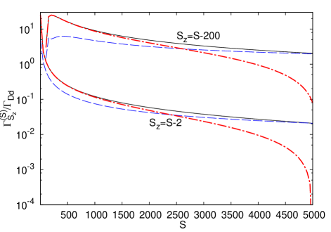
Figure 1: The total decay rates for the state with the total spin $S$ and its projection $S_{z}$ for two values of $S-S_{z}$. The solid black lines correspond to the background scattering lengths. The dashed blue and dot-dashed red lines show the decay rates minimized by tuning of $a_{\downdownarrows}$ and $a_{\uparrow\downarrow}$, respectively.

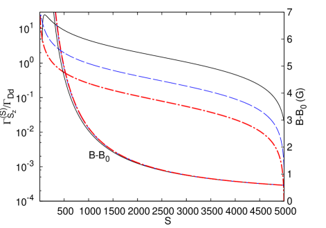
Figure 2: The total decay rates for the state with the total spin $S$ and its projection $S_{z}$ minimized by $a_{\uparrow\downarrow}$ tuning in the vicinity of the Feshbach resonance at $B_{0}\approx 9.13\mathrm{G}$ in ⁸⁷Rb. The solid black, dashed blue, and dot-dashed red lines correspond to $S-S_{z}=100$, 20, and 5, respectively. The plots of optimal detuning $B-B_{0}$ for different $S-S_{z}$ almost coincide.

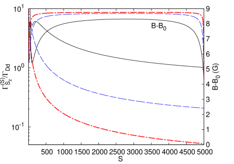
Figure 3: The total decay rates for the state of $N=10^{4}$ atoms of ⁸⁷Rb with the total spin $S$ and its projection $S_{z}$ minimized by $a_{\downdownarrows}$ tuning in the vicinity of the Feshbach resonance at $B_{0}\approx 1007.4\mathrm{G}$. The solid black, dashed blue, and dot-dashed red lines correspond to $S-S_{z}=100$, 20, and 5, respectively. The optimal detuning $B-B_{0}$ for different $S-S_{z}$ is presented by three upper plots.

The total decay rate $\Gamma_{S_{z}}^{(S)}=\sum_{S^{\prime}\neq S}\Gamma_{S_{z}}^{(S,S^{\prime})}$ is presented in Fig. 1. Even for $N=10^{4}$ atoms it does not exceed $\approx 60\Gamma_{Dd}$. The decay is suppressed at large values of $S$ and $S_{z}$.

The Feshbach resonance tuning of the elastic scattering length Chin et al. (2010) cannot eliminate the decay, as one tuning parameter — the magnetic field — cannot make vanish two combination of the scattering lengths — $\alpha_{+}$ and $\alpha_{-}$. However, the Feshbach tuning can minimize the decay due to the destructive interference of the contributions of the spherical vector and tensor interactions, mentioned above. These contributions are proportional to $\alpha_{-}$ and $\alpha_{+}$, respectively, in Eq. (15). In the case of ⁸⁷Rb, the resonance in $\uparrow\downarrow$ collision at $B_{0}\approx 9.13\mathrm{G}$ (with the width $\Delta\approx 15\mathrm{mG}$) is well separated from the resonances in $\downarrow\downarrow$ collisions at $B_{0}>400\mathrm{G}$ (the widest one at $B_{0}\approx 1007.4\mathrm{G}$ has $\Delta\approx 0.21\mathrm{G}$) Chin et al. (2010). No resonances are known in $\uparrow\uparrow$ collisions. Then either $a_{\uparrow\downarrow}$ or $a_{\downdownarrows}$ can be tuned without changing other scattering lengths. The resulting decay rates are presented in Fig. 1. Tuning of $a_{\downdownarrows}$ can reduce the decay rate at small $S$, while tuning of $a_{\uparrow\downarrow}$ can lead to the reduction by orders of magnitude at large $S$ and $S_{z}$. The magnetic field detunings, minimizing the decay rates, and the minimal rates are plotted in Figs. 2 and 3. Even the minimal detunings $0.5\mathrm{G}$ and $4\mathrm{G}$, respectively, substantially exceeds the resonance widths. Then the closed-channel effects can be neglected, although the resonances are closed-channel dominated Chin et al. (2010). The resonance-enhancement of three-body losses (see Yurovsky and Ben-Reuven (2003)) can be neglected at such detunings as well.

Approximate expressions can be obtained in the regions of maximal suppression, $S_{z}\approx\pm S$. Here the $a_{\uparrow\downarrow}$ tuning minimizes the decay rate when $\alpha_{+}\approx\mp\alpha_{-}$ and the minimal rate is approximated for $N\gg 1$ by

$$\Gamma_{S_{z}}^{(S)}\approx\frac{2\alpha_{+}^{2}\Gamma_{Dd}}{N(2S+3)}\biggl{\{}2(N-2S)(N-2S-2)\\ -\frac{S-|S_{z}|}{S+1}\left[2N^{2}-(N-2S)N(4S+5)\right]\biggr{\}}.$$

Then for $N/2-S=\mathrm{const}\ll N$, $S-|S_{z}|=\mathrm{const}$, and fixed density the decay rate is scaled as $1/N$. The desired scattering lengths, $a_{\uparrow\downarrow}\approx a_{\upuparrows}$ at $S_{z}\approx S$, or $a_{\uparrow\downarrow}\approx a_{\downdownarrows}$ at $S_{z}\approx-S$ , are obtained for ⁸⁷Rb at $B-B_{0}\approx 0.6G$ or $-0.6G$, respectively. The state with $S=S_{z}=N/2$ for even $N$ (or with $S=S_{z}=(N-1)/2$ for odd $N$ ) cannot decay to states with $S^{\prime}<S$ since $S^{\prime}$ cannot be less than $S_{z}$, nor to states with $S^{\prime}>S$ since $S^{\prime}$ cannot exceed $N/2$.

When the decay rates are substantially suppressed, the lifetime of the states with well-defined spins is restricted by the loss processes in the cold gas, such as spin-changing (dipolar relaxation) and three-body collisions, leading to high-energy atoms escaping the trap. The spin-changing collisions can also change many-body spin and its projection, leading to additional decay. However, this decay, having the rate comparable to the gas loss rate, does not lead to additional restriction of the lifetime of the states with well-defined spins. In real physical situations, dipolar relaxation becomes substantial only for Cs and atoms with high magnetic momenta Stamper-Kurn and Ueda (2013).

Conclusions

Spatially-chaotic many-body eigenstates of the total spin operator can be described, according to the Berry conjecture Berry (1977), within the Srednicki approach Srednicki (1994) [see Eq. (11)]. This description, in a combination with the sum rules Yurovsky (2015b), allows us to evaluate the matrix elements of spin-dependent two-body interactions, leading to transitions between states with different total spins. The transition rates, calculated within the Weisskopf-Wigner approach (15), are proportional to the elastic collision rate per particle (16). The decay rates can be suppressed due to destructive interference of the contributions the spherical vector and tensor terms in the spin-dependent interaction $\hat{V}_{\mathrm{spin}}$. The interference terms in Eq. (15) can be controlled by Feshbach resonances as they are proportional to $\alpha_{+}\alpha_{-}$. Another manifestation of quantum interference is the effect of dynamical localization. It can slow down relaxation due to periodic driving Das (2010); Roy and Das (2015); Cem Keser et al. , while the present mechanism pertains to time-independent systems. The long-lived entangled states can find applications in quantum computation and metrology.

Appendix A Wavefunctions with defined total spins of interacting and non-interacting particles

A permutation of coordinates in the wavefunction (10) can be represented as

$$\mathcal{P}\Phi_{tn}^{(S)}\propto\sum_{\{\mathbf{p}\}}A_{n}^{(S)}(t,\{\mathbf{p}\})\tilde{\delta}(\{\mathbf{p}\}^{2}-2mE_{n}^{(S)})\\ \times\exp(i\sum_{j}\mathbf{p}_{\mathcal{P}^{-1}j}\mathbf{r}_{j}/\hbar)\\ \propto\sum_{\{\mathbf{p}\}}A_{n}^{(S)}(t,\mathcal{P}\{\mathbf{p}\})\tilde{\delta}(\{\mathbf{p}\}^{2}-2mE_{n}^{(S)})\\ \times\exp(i\sum_{j}\mathbf{p}_{j}\mathbf{r}_{j}/\hbar),$$

where $\mathcal{P}\{\mathbf{p}\}\equiv\{\mathbf{p}_{\mathcal{P}1},\ldots,\mathbf{p}_{\mathcal{P}N}\}$. Then Eq. (6) leads to

$$A_{n}^{(S)}(t,\mathcal{P}\{\mathbf{p}\})=\sum_{r}D_{rt}^{[\lambda]}(\mathcal{P})A_{n}^{(S)}(r,\{\mathbf{p}\})$$ (17)

Let us represent the wavefunction $\Phi_{tn}^{(S)}$ in the form which explicitly shows its permutation properties. This can be done by summation in Eq. (10) over the simplex $\mathbf{p}_{1}<\mathbf{p}_{2}<\cdots<\mathbf{p}_{N}$. Momentum sets in other simplices are given by $\mathcal{P}\{\mathbf{p}\}$. Neglecting contributions of the sets $\{\mathbf{p}\}$ which contain equal momenta $\mathbf{p}_{j}=\mathbf{p}_{j^{\prime}}$, one gets

$$\Phi_{tn}^{(S)}\propto\sum_{\mathcal{P}}{\sum_{\{\mathbf{p}\}}}^{\prime}A_{n}^{(S)}(t,\mathcal{P}\{\mathbf{p}\})\tilde{\delta}(\{\mathbf{p}\}^{2}-2mE_{n}^{(S)})\\ \times\exp(i\sum_{j}\mathbf{p}_{\mathcal{P}j}\mathbf{r}_{j}/\hbar)\\ \propto{\sum_{\{\mathbf{p}\}}}^{\prime}\sum_{r}A_{n}^{(S)}(r,\{\mathbf{p}\})\tilde{\delta}(\{\mathbf{p}\}^{2}-2mE_{n}^{(S)})\sum_{\mathcal{P}}D_{rt}^{[\lambda]}(\mathcal{P})\\ \times\exp(i\sum_{j}\mathbf{p}_{j}\mathbf{r}_{\mathcal{P}^{-1}j}/\hbar)\\ \propto{\sum_{\{\mathbf{p}\}}}^{\prime}\sum_{r}A_{n}^{(S)}(r,\{\mathbf{p}\})\tilde{\delta}(\{\mathbf{p}\}^{2}-2mE_{n}^{(S)})\left(\frac{N!}{f_{S}}\right)^{1/2}\tilde{\Phi}_{tr\{\mathbf{p}\}}^{(S)}.$$ (18)

Here Eq. (17) and the identity for the orthogonal representation matrices $D_{rt}^{[\lambda]}(\mathcal{P}^{-1})=D_{tr}^{[\lambda]}(\mathcal{P})$ are used and

$$\tilde{\Phi}_{tr\{\mathbf{p}\}}^{(S)}=\left(\frac{f_{S}}{N!}\right)^{1/2}\sum_{\mathcal{P}}D_{tr}^{[\lambda]}(\mathcal{P})\exp(i\sum_{j}\mathbf{p}_{j}\mathbf{r}_{\mathcal{P}j}/\hbar)$$

are spatial wavefunctions of non-interacting particles Kaplan (1975); Pauncz (1995); Yurovsky (2015a). They satisfy relations (6), forming a basis of the irreducible representation associated with $\lambda$. The Young tableau $r$ labels different representations for the same $S$ and $\{\mathbf{p}\}$. The total wavefunction of non-interacting particles

$$\tilde{\Psi}_{r\{\mathbf{p}\}S_{z}}^{(S)}=f_{S}^{-1/2}\sum_{t}\tilde{\Phi}_{tr\{\mathbf{p}\}}^{(S)}\Xi_{tS_{z}}^{(S)}$$ (19)

is expressed similarly to $\Psi_{nS_{z}}^{(S)}$ [see Eq. (5)]. Then Eq. (18) leads to Eq. (11). The wavefunctions of non-interacting particles form an orthonormal basis

$$\left\langle\tilde{\Psi}_{r^{\prime}\{\mathbf{p^{\prime}}\}S^{\prime}_{z}}^{(S^{\prime})}|\tilde{\Psi}_{r\{\mathbf{p}\}S_{z}}^{(S)}\right\rangle=\delta_{S^{\prime}S}\delta_{S^{\prime}_{z}S_{z}}\delta_{r^{\prime}r}\delta_{\{\mathbf{p^{\prime}}\}\{\mathbf{p}\}}$$ (20)

and satisfy the Schrödinger equation

$$\hat{H}_{0}\tilde{\Psi}_{r\{\mathbf{p}\}S_{z}}^{(S)}=\frac{1}{2m}\{\mathbf{p}\}^{2}\tilde{\Psi}_{r\{\mathbf{p}\}S_{z}}^{(S)}.$$

Appendix B Two- and four-point correlation functions of the coefficients $A_{n}^{(S)}(r,\{\mathbf{p}\})$

According to the Berry conjecture Berry (1977), the coefficients $A_{n}^{(S)}(t,\{\mathbf{p}\})$ in Eqs. (10) and (11) can be treated as Gaussian random variables with a two-point correlation function Srednicki (1994)

$$\left\langle{A_{n^{\prime}}^{(S^{\prime})}}^{*}(t^{\prime},\{\mathbf{p^{\prime}}\})A_{n}^{(S)}(t,\{\mathbf{p}\})\right\rangle_{\mathrm{EE}}=\frac{\delta_{S^{\prime}S}\delta_{n^{\prime}n}\delta_{\{\mathbf{p^{\prime}}\}\{\mathbf{p}\}}f(t,t^{\prime})}{\tilde{\delta}(\{\mathbf{p^{\prime}}\}^{2}-\{\mathbf{p}\}^{2})},$$ (21)

where ${A_{n}^{(S)}}^{*}(t,\{\mathbf{p}\})=A_{n}^{(S)}(t,\{\mathbf{-p}\})$. The Kronecker symbols appear here since different $S$ and $n$ correspond to different (independent) eigenfunctions and different $\{\mathbf{p}\}$ within the given simplex correspond to different (independent) plane waves. (The correlation functions with $\{\mathbf{p}\}$ and $\{\mathbf{p^{\prime}}\}$ in different simplices do not appear within the present paper.) By now nothing can be told on $f(t,t^{\prime})$, since $\Phi_{tn}^{(S)}$ and $\Phi_{t^{\prime}n}^{(S)}$ are components of the same eigenfunction, related by Eq. (6). The factors $f(t,t^{\prime})$ are determined below.

Equation (17) leads to the following equality for an arbitrary permutation $\mathcal{P}$

$$A_{n}^{(S)}(t,\{\mathbf{p}\})=\sum_{r}D_{tr}^{[\lambda]}(\mathcal{P})A_{n}^{(S)}(r,\mathcal{P}\{\mathbf{p}\}).$$

It relates coefficients $A_{n}^{(S)}(r,\{\mathbf{p}\})$ in different simplices and leads to

$$\left\langle{A_{n}^{(S)}}^{*}(t^{\prime},\{\mathbf{p}\})A_{n}^{(S)}(t,\{\mathbf{p}\})\right\rangle_{\mathrm{EE}}\\ =\sum_{r,r^{\prime}}D_{t^{\prime}r^{\prime}}^{[\lambda]}(\mathcal{P})D_{tr}^{[\lambda]}(\mathcal{P})\left\langle{A_{n}^{(S)}}^{*}(r^{\prime},\mathcal{P}\{\mathbf{p}\})A_{n}^{(S)}(r,\mathcal{P}\{\mathbf{p}\})\right\rangle_{\mathrm{EE}}.$$

Applying Eq. (21) to all correlation functions, we get

$$f(t,t^{\prime})=\sum_{r,r^{\prime}}D_{t^{\prime}r^{\prime}}^{[\lambda]}(\mathcal{P})D_{tr}^{[\lambda]}(\mathcal{P})f(r,r^{\prime})$$ (22)

for any $\mathcal{P}$. Averaging the right hand side of this equation over all $\mathcal{P}$ and using the orthogonality relationKaplan (1975); Pauncz (1995)

$$\sum_{\mathcal{P}}D_{t^{\prime}r^{\prime}}^{[\lambda^{\prime}]}(\mathcal{P})D_{tr}^{[\lambda]}(\mathcal{P})=\frac{N!}{f_{S}}\delta_{tt^{\prime}}\delta_{rr^{\prime}}\delta_{\lambda\lambda^{\prime}},$$

one gets the equation

$$f(t,t^{\prime})=\frac{1}{f_{S}}\delta_{tt^{\prime}}\sum_{r}f(r,r).$$

Its solution is $f(t,t^{\prime})=\mathrm{const}\delta_{tt^{\prime}}$. Equation (12) is obtained if $\mathrm{const}=1$. Other choice of the constant factor can only change the normalization factor in Eq. (11). The function $f(t,t^{\prime})=\delta_{tt^{\prime}}$ satisfies Eq. (22), as can be easily proven using the identity

$$\sum_{r}D_{t^{\prime}r}^{[\lambda]}(\mathcal{P})D_{tr}^{[\lambda]}(\mathcal{P})=D_{t^{\prime}t}^{[\lambda]}(\mathcal{P}\mathcal{P}^{-1})=\delta_{t^{\prime}t}$$ (23)

for the Young orthogonal matrices (see Kaplan (1975); Pauncz (1995)).

The relation between four-point and two-point correlation functions

$$\left\langle A_{n^{\prime\prime\prime}}^{(S^{\prime\prime\prime})}(t^{\prime\prime\prime},\{\mathbf{p^{\prime\prime\prime}}\})A_{n^{\prime\prime}}^{(S^{\prime\prime})}(t^{\prime\prime},\{\mathbf{p^{\prime\prime}}\})A_{n^{\prime}}^{(S^{\prime})}(t^{\prime},\{\mathbf{p^{\prime}}\})A_{n}^{(S)}(t,\{\mathbf{p}\})\right\rangle_{\mathrm{EE}}\\ =\left\langle A_{n^{\prime\prime\prime}}^{(S^{\prime\prime\prime})}(t^{\prime\prime\prime},\{\mathbf{p^{\prime\prime\prime}}\})A_{n^{\prime\prime}}^{(S^{\prime\prime})}(t^{\prime\prime},\{\mathbf{p^{\prime\prime}}\})\right\rangle_{\mathrm{EE}}\left\langle A_{n^{\prime}}^{(S^{\prime})}(t^{\prime},\{\mathbf{p^{\prime}}\})A_{n}^{(S)}(t,\{\mathbf{p}\})\right\rangle_{\mathrm{EE}}\\ +\left\langle A_{n^{\prime\prime\prime}}^{(S^{\prime\prime\prime})}(t^{\prime\prime\prime},\{\mathbf{p^{\prime\prime\prime}}\})A_{n^{\prime}}^{(S^{\prime})}(t^{\prime},\{\mathbf{p^{\prime}}\})\right\rangle_{\mathrm{EE}}\left\langle A_{n^{\prime\prime}}^{(S^{\prime\prime})}(t^{\prime\prime},\{\mathbf{p^{\prime\prime}}\})A_{n}^{(S)}(t,\{\mathbf{p}\})\right\rangle_{\mathrm{EE}}\\ +\left\langle A_{n^{\prime\prime}}^{(S^{\prime\prime})}(t^{\prime\prime},\{\mathbf{p^{\prime\prime}}\})A_{n^{\prime}}^{(S^{\prime})}(t^{\prime},\{\mathbf{p^{\prime}}\})\right\rangle_{\mathrm{EE}}\left\langle A_{n^{\prime\prime\prime}}^{(S^{\prime\prime\prime})}(t^{\prime\prime\prime},\{\mathbf{p^{\prime\prime\prime}}\})A_{n}^{(S)}(t,\{\mathbf{p}\})\right\rangle_{\mathrm{EE}}$$ (24)

is a straightforward generalization of the similar relation in Srednicki (1994). For the product of four coefficients $A_{n}^{(S)}(r,\{\mathbf{p}\})$ in Eq. (14) it leads to

$$\left\langle{A_{n^{\prime}}^{(S^{\prime})}}^{*}(r^{\prime},\{\mathbf{p^{\prime}}\})A_{n}^{(S)}(r,\{\mathbf{p}\}){A_{n}^{(S)}}^{*}(r^{\prime\prime},\{\mathbf{p^{\prime\prime}}\})A_{n^{\prime}}^{(S^{\prime})}(r^{\prime\prime\prime},\{\mathbf{p^{\prime\prime\prime}}\})\right\rangle_{\mathrm{EE}}=\frac{\delta_{r^{\prime\prime}r}\delta_{\{\mathbf{p^{\prime\prime}}\}\{\mathbf{p}\}}\delta_{r^{\prime\prime\prime}r^{\prime}}\delta_{\{\mathbf{p^{\prime\prime\prime}}\}\{\mathbf{p^{\prime}}\}}}{\tilde{\delta}(\{\mathbf{p^{\prime\prime}}\}^{2}-\{\mathbf{p}\}^{2})\tilde{\delta}(\{\mathbf{p^{\prime\prime\prime}}\}^{2}-\{\mathbf{p^{\prime}}\}^{2})}$$ (25)

since $S^{\prime}\neq S$.

Appendix C Normalization factor and the density of states

Orthonormality of the non-interacting particle wavefunctions (20) leads, using the two-point correlation functions (12), to the following overlap of the wavefunctions of interacting particles (11)

$$\left\langle\left\langle\Psi_{n^{\prime}S^{\prime}_{z}}^{(S^{\prime})}|\Psi_{nS_{z}}^{(S)}\right\rangle\right\rangle_{\mathrm{EE}}=\left(\mathcal{N}_{n}^{(S)}\right)^{2}f_{S}\delta_{S^{\prime}_{z}S_{z}}\delta_{S^{\prime}S}\delta_{n^{\prime}n}\\ \times{\sum_{\{\mathbf{p}\}}}^{\prime}\tilde{\delta}(\{\mathbf{p}\}^{2}-2mE_{n}^{(S)}).$$ (26)

The summation over $\{\mathbf{p}\}$ in the simplex can be approximated by integration over whole momentum space with the replacement of $\tilde{\delta}$ by the Dirac $\delta$-function,

$${\sum_{\{\mathbf{p}\}}}^{\prime}\tilde{\delta}(\{\mathbf{p}\}^{2}-2mE_{n}^{(S)})\approx\frac{1}{N!}\left(\frac{L}{2\pi\hbar}\right)^{DN}\\ \times\int d^{DN}p\delta(\{\mathbf{p}\}^{2}-2mE_{n}^{(S)})$$ (27)

The integral

$$\int d^{DN}p\delta(\{\mathbf{p}\}^{2}-E)=\frac{(\pi E)^{DN/2}}{\Gamma(DN/2)E}$$ (28)

is calculated in Srednicki (1994). Then the normalization factor is given by

$$\left(\mathcal{N}_{n}^{(S)}\right)^{-2}=\frac{f_{S}L^{DN}(mE_{n}^{(S)})^{DN/2-1}}{2N!(2\pi)^{DN/2}\Gamma(DN/2)\hbar^{DN}}.$$ (29)

The density of states of interacting particles can be approximated by the one of non-interacting ones. Number of such states with the total spin $S$ below the energy $E$ is

$$n^{(S)}(E)=f_{S}{\sum_{\{\mathbf{p}\}}}^{\prime}\Theta(E-\{\mathbf{p}\}^{2}/(2m)).$$

Then the density of states is estimated as

$$\frac{dn^{(S)}(E)}{dE}\approx\frac{n^{(S)}(E+\varDelta)-n^{(S)}(E-\varDelta)}{2\varDelta}\\ =f_{S}{\sum_{\{\mathbf{p}\}}}^{\prime}\tilde{\delta}(E-\{\mathbf{p}\}^{2}/(2m))=2m\left(\mathcal{N}_{n}^{(S)}\right)^{-2}$$ (30)

[cf. Eq. (26)].

Appendix D Matrix elements and decay rates

If the scattering lengths $a_{\sigma\sigma^{\prime}}$ and interaction strengths $g_{Dd}^{\sigma\sigma^{\prime}}$ are spin-dependent, states with different total spins become coupled by the spherical vector $\hat{V}_{0}$ and tensor $\hat{V}_{0}^{(2)}$ interactions in Eq. (4). Matrix elements of the spherical vector and tensor are related to ones for the maximal allowed spin projections by the Wigner-Eckart theorem Yurovsky (2015a, b),

$$\langle\Psi_{n^{\prime}S_{z}}^{(S^{\prime})}|\hat{V}_{0}|\Psi_{nS_{z}}^{(S)}\rangle= X_{S_{z}0}^{(S,S^{\prime},1)}\langle\Psi_{n^{\prime}S^{\prime}}^{(S^{\prime})}|\hat{V}_{S^{\prime}-S}|\Psi_{nS}^{(S)}\rangle$$ (31)

$$\langle\Psi_{n^{\prime}S_{z}}^{(S^{\prime})}|\hat{V}_{0}^{(2)}|\Psi_{nS_{z}}^{(S)}\rangle= X_{S_{z}0}^{(S,S^{\prime},2)}\langle\Psi_{n^{\prime}S^{\prime}}^{(S^{\prime})}|\hat{V}_{S^{\prime}-S}^{(2)}|\Psi_{nS}^{(S)}\rangle,$$

and do not vanish for $|S-S^{\prime}|\leq 1$ and $|S-S^{\prime}|\leq 2$, respectively. Here the ratios of the $3j$ Wigner symbols $X_{S_{z}0}^{(S,S^{\prime},q)}$ are tabulated in Yurovsky (2015a, b). Matrix elements with $S^{\prime}>S$ are calculated using Hermitian conjugate in Eq. (31), taking into account that $(\hat{V}_{0})^{\dagger}=\hat{V}_{0}$, $(\hat{V}_{0}^{(2)})^{\dagger}=\hat{V}_{0}^{(2)}$, $\hat{V}_{-1}^{\dagger}=-\hat{V}_{+1}$, $(\hat{V}_{-1}^{(2)})^{\dagger}=-\hat{V}_{+1}^{(2)}$, and $(\hat{V}_{-2}^{(2)})^{\dagger}=\hat{V}_{+2}^{(2)}$ (see Yurovsky (2015b)).

Sums of the products of the matrix elements of the spherical tensors between the wavefunctions of non-interacting particles (19) can be represented for $S^{\prime}\leq S$ as Yurovsky (2015b)

$$\sum_{r,r^{\prime}}\langle\tilde{\Psi}_{r^{\prime}\{\mathbf{p}^{\prime}\}S^{\prime}}^{(S^{\prime})}|\hat{V}_{a}|\tilde{\Psi}_{r\{\mathbf{p}\}S}^{(S)}\rangle\langle\tilde{\Psi}_{r^{\prime}\{\mathbf{p}^{\prime}\}S^{\prime}}^{(S^{\prime})}|\hat{V}_{b}|\tilde{\Psi}_{r\{\mathbf{p}\}S}^{(S)}\rangle^{*}\\ =Y^{(S,2)}[\hat{V}_{a},\hat{V}_{b}]\frac{2f_{S^{\prime}}}{N(N-1)}\sum_{j<j^{\prime}}|\langle\mathbf{p}^{\prime}_{j}\mathbf{p}^{\prime}_{j^{\prime}}|\delta|\mathbf{p}_{j}\mathbf{p}_{j^{\prime}}\rangle|^{2}\\ \times\prod_{j^{\prime}\neq j^{\prime\prime}\neq j}\delta_{\mathbf{p}^{\prime}_{j^{\prime\prime}}\mathbf{p}_{j^{\prime\prime}}}$$ (32)

Here the universal factors $Y^{(S,2)}[\hat{V}_{a},\hat{V}_{b}]$ are independent of the occupied spatial modes, while the sum of matrix elements is independent of the total spin and its projection. The sum rule (32) is valid if the sets $\{\mathbf{p}\}$ and $\{\mathbf{p}^{\prime}\}$ are different by two momenta. Similar sum for $\{\mathbf{p}^{\prime}\}=\{\mathbf{p}\}$ is proportional to deviations of the matrix elements $\langle\mathbf{p}^{\prime}\mathbf{p}|\delta|\mathbf{p}\mathbf{p}^{\prime}\rangle$ from their average values Yurovsky (2015b) and vanish in the present case since

$$\langle\mathbf{p}^{\prime}_{j}\mathbf{p}^{\prime}_{j^{\prime}}|\delta|\mathbf{p}_{j}\mathbf{p}_{j^{\prime}}\rangle=L^{-D}\delta_{\mathbf{p}^{\prime}_{j}+\mathbf{p}^{\prime}_{j^{\prime}}\mathbf{p}_{j}+\mathbf{p}_{j^{\prime}}}$$

and the matrix elements $\langle\mathbf{p}^{\prime}\mathbf{p}|\delta|\mathbf{p}\mathbf{p}^{\prime}\rangle=L^{-D}$ are constant. The sets $\{\mathbf{p}\}$ and $\{\mathbf{p}^{\prime}\}$ different by single momentum are not coupled due to the momentum conservation.

The form (32) of the sum implies that the unchanged momenta are in the same positions in the sets $\{\mathbf{p}\}$ and $\{\mathbf{p}^{\prime}\}$. However, arbitrary permutations $\mathcal{P}$ and $\mathcal{P}^{\prime}$ of the momentum sets do not change the sum,

$$\sum_{r,r^{\prime}}\langle\tilde{\Psi}_{r^{\prime}\mathcal{P}^{\prime}\{\mathbf{p}^{\prime}\}S^{\prime}}^{(S^{\prime})}|\hat{V}_{a}|\tilde{\Psi}_{r\mathcal{P}\{\mathbf{p}\}S}^{(S)}\rangle\langle\tilde{\Psi}_{r^{\prime}\mathcal{P}^{\prime}\{\mathbf{p}^{\prime}\}S^{\prime}}^{(S^{\prime})}|\hat{V}_{b}|\tilde{\Psi}_{r\mathcal{P}\{\mathbf{p}\}S}^{(S)}\rangle^{*}\\ =\sum_{r,r^{\prime}}\langle\tilde{\Psi}_{r^{\prime}\{\mathbf{p}^{\prime}\}S^{\prime}}^{(S^{\prime})}|\hat{V}_{a}|\tilde{\Psi}_{r\{\mathbf{p}\}S}^{(S)}\rangle\langle\tilde{\Psi}_{r^{\prime}\{\mathbf{p}^{\prime}\}S^{\prime}}^{(S^{\prime})}|\hat{V}_{b}|\tilde{\Psi}_{r\{\mathbf{p}\}S}^{(S)}\rangle^{*}.$$ (33)

This equality is provided by the transformation of the non-interacting particle wavefunctions on permutation of the quantum numbers (see Kaplan (1975))

$$\tilde{\Psi}_{r\mathcal{P}\{\mathbf{p}\}S}^{(S)}=\sum_{r^{\prime}}D_{r^{\prime}r}^{[\lambda]}(\mathcal{P})\tilde{\Psi}_{r^{\prime}\{\mathbf{p}\}S}^{(S)}$$

and the identity (23). Then the sum rule (32) can be rewritten as

$$\sum_{r,r^{\prime}}\langle\tilde{\Psi}_{r^{\prime}\{\mathbf{p}^{\prime}\}S^{\prime}}^{(S^{\prime})}|\hat{V}_{a}|\tilde{\Psi}_{r\{\mathbf{p}\}S}^{(S)}\rangle\langle\tilde{\Psi}_{r^{\prime}\{\mathbf{p}^{\prime}\}S^{\prime}}^{(S^{\prime})}|\hat{V}_{b}|\tilde{\Psi}_{r\{\mathbf{p}\}S}^{(S)}\rangle^{*}\\ =Y^{(S,2)}[\hat{V}_{a},\hat{V}_{b}]\frac{f_{S^{\prime}}}{N(N-1)}\sum_{\mathcal{P}}\sum_{j<j^{\prime}}|\langle\mathbf{p}^{\prime}_{\mathcal{P}j}\mathbf{p}^{\prime}_{\mathcal{P}j^{\prime}}|\delta|\mathbf{p}_{j}\mathbf{p}_{j^{\prime}}\rangle|^{2}\\ \times\prod_{j^{\prime}\neq j^{\prime\prime}\neq j}\delta_{\mathbf{p}^{\prime}_{\mathcal{P}j^{\prime\prime}}\mathbf{p}_{j^{\prime\prime}}}.$$ (34)

The factor $2$ in Eq. (32) is absent here since the Kronecker symbols are satisfied by two permutations, $\mathcal{P}$ and $\mathcal{P}\mathcal{P}_{jj^{\prime}}$, when the momenta $\mathbf{p}_{j}$ and $\mathbf{p}_{j^{\prime}}$ are changed.

In the matrix element (14) between the wavefunctions of interacting particles, we can replace the sum over $\{\mathbf{p}\}$ in the simplex $\mathbf{p}_{1}<\mathbf{p}_{2}<\cdots<\mathbf{p}_{N}$ by average of sums over all simplices, $\mathbf{p}_{\mathcal{P}1}<\mathbf{p}_{\mathcal{P}2}<\cdots<\mathbf{p}_{\mathcal{P}N}$,

$${\sum_{\{\mathbf{p}\}}}^{\prime}F(\{\mathbf{p}\})=\frac{1}{N!}\sum_{\mathcal{P}}{\sum_{\mathcal{P}\{\mathbf{p}\}}}^{\prime}F(\mathcal{P}\{\mathbf{p}\}).$$

Since the sums of the matrix elements (34) and sums of squared momenta $\{\mathbf{p}\}^{2}$ are invariant over momentum permutations, Eq. (14) takes the form

$$\left\langle|\langle\Psi_{n^{\prime}S^{\prime}_{z}}^{(S^{\prime})}|\hat{V}_{\mathrm{spin}}|\Psi_{nS_{z}}^{(S)}\rangle|^{2}\right\rangle_{\mathrm{EE}}=\left(\frac{\mathcal{N}_{n}^{(S)}\mathcal{N}_{n^{\prime}}^{(S^{\prime})}}{N!}\right)^{2}\\ \times{\sum_{\{\mathbf{p}\}}}^{\prime\prime}{\sum_{\{\mathbf{p^{\prime}}\}}}^{\prime\prime}\tilde{\delta}(\{\mathbf{p}\}^{2}-2mE_{n}^{(S)})\tilde{\delta}(\{\mathbf{p^{\prime}}\}^{2}-2mE_{n^{\prime}}^{(S^{\prime})})\\ \times\sum_{r,r^{\prime}}|\langle\tilde{\Psi}_{r^{\prime}\{\mathbf{p}^{\prime}\}S^{\prime}_{z}}^{(S^{\prime})}|\hat{V}_{\mathrm{spin}}|\tilde{\Psi}_{r\{\mathbf{p}\}S_{z}}^{(S)}\rangle|^{2}.$$ (35)

where $\sum_{\{\mathbf{p}\}}^{\prime\prime}$ denotes summation over the sets $\{\mathbf{p}\}$ which do not contain equal momenta.

The Weisskopf-Wigner decay rates (13) for transitions from the $S$-multiplet to the $S^{\prime}$ one, $\Gamma_{S_{z}}^{(S,S^{\prime})}$, calculated with the matrix elements (35) of the operator (4), relations (31), and sum rules (34) attain the form

$$\Gamma_{S_{z}}^{(S,S-1)}=\biggl{[}\frac{2}{3}\left(\alpha_{+}X_{S_{z}0}^{(S,S-1,2)}\right)^{2}Y^{(S,2)}[\hat{V}_{-1}^{(2)},\hat{V}_{-1}^{(2)}]\\ +2\sqrt{\frac{2}{3}}\alpha_{+}\alpha_{-}X_{S_{z}0}^{(S,S-1,2)}X_{S_{z}0}^{(S,S-1,1)}Y^{(S,2)}[\hat{V}_{-1}^{(2)},\hat{V}_{-1}]\\ +\left(\alpha_{-}X_{S_{z}0}^{(S,S-1,1)}\right)^{2}Y^{(S,2)}[\hat{V}_{-1},\hat{V}_{-1}]\biggr{]}\frac{f_{S-1}}{Nf_{S}}\Gamma_{Dd}$$ (36a)

$$\Gamma_{S_{z}}^{(S,S+1)}=\biggl{[}\frac{2}{3}\left(\alpha_{+}X_{S_{z}0}^{(S+1,S,2)}\right)^{2}Y^{(S+1,2)}[\hat{V}_{-1}^{(2)},\hat{V}_{-1}^{(2)}]\\ +2\sqrt{\frac{2}{3}}\alpha_{+}\alpha_{-}X_{S_{z}0}^{(S+1,S,2)}X_{S_{z}0}^{(S+1,S,1)}Y^{(S+1,2)}[\hat{V}_{-1}^{(2)},\hat{V}_{-1}]\\ +\left(\alpha_{-}X_{S_{z}0}^{(S+1,S,1)}\right)^{2}Y^{(S+1,2)}[\hat{V}_{-1},\hat{V}_{-1}]\biggr{]}\frac{1}{N}\Gamma_{Dd}$$ (36b)

$$\Gamma_{S_{z}}^{(S,S-2)}=\frac{2}{3}\left(\alpha_{+}X_{S_{z}0}^{(S,S-2,2)}\right)^{2}Y^{(S,2)}[\hat{V}_{-2}^{(2)},\hat{V}_{-2}^{(2)}]\frac{f_{S-2}}{Nf_{S}}\Gamma_{Dd}$$ (36c)

$$\Gamma_{S_{z}}^{(S,S+2)}=\frac{2}{3}\left(\alpha_{+}X_{S_{z}0}^{(S+2,S,2)}\right)^{2}Y^{(S+2,2)}[\hat{V}_{-2}^{(2)},\hat{V}_{-2}^{(2)}]\frac{1}{N}\Gamma_{Dd}$$ (36d)

Here the factor $\Gamma_{Dd}$ is independent of $S$, $S^{\prime}$, and $S_{z}$, as will be explicitly seen below. It is obtained from Eqs. (13), (35), and (34) as

$$\Gamma_{Dd}=\frac{\pi f_{S}Ng_{Dd}^{2}}{2\hbar L^{2D}}\left(\frac{\mathcal{N}_{n}^{(S)}\mathcal{N}_{n^{\prime}}^{(S^{\prime})}}{N!}\right)^{2}\frac{dn^{(S^{\prime})}(E_{n^{\prime}}^{(S^{\prime})})}{dE}|_{E_{n^{\prime}}^{(S^{\prime})}=E_{n}^{(S)}}\\ \times{\sum_{\{\mathbf{p}\}\neq\{\mathbf{p^{\prime}}\}}}^{\prime\prime}\tilde{\delta}(\{\mathbf{p}\}^{2}-2mE_{n}^{(S)})\tilde{\delta}(\{\mathbf{p^{\prime}}\}^{2}-2mE_{n^{\prime}}^{(S^{\prime})})\\ \times\frac{1}{N(N-1)}\sum_{j<j^{\prime}}\sum_{\mathcal{P}}\delta_{\mathbf{p}^{\prime}_{\mathcal{P}j}+\mathbf{p}^{\prime}_{\mathcal{P}j^{\prime}}\mathbf{p}_{j}+\mathbf{p}_{j^{\prime}}}\prod_{j^{\prime}\neq j^{\prime\prime}\neq j}\delta_{\mathbf{p}^{\prime}_{\mathcal{P}j^{\prime\prime}}\mathbf{p}_{j^{\prime\prime}}}.$$

The Kronecker symbols here fix values of all $\mathbf{p^{\prime}}$, except for $\mathbf{p}^{\prime}_{j}-\mathbf{p}^{\prime}_{j^{\prime}}$. The relation (30) between the density of states and the normalization factor and replacement summation by interaction lead to

$$\Gamma_{Dd}=\frac{\pi mg_{Dd}^{2}}{2\hbar L^{2D}N!}\left(\frac{L}{2\pi\hbar}\right)^{D(N+1)}(\mathcal{N}_{n}^{(S)})^{2}Nf_{S}\\ \times\int d^{DN}p\delta(\{\mathbf{p}\}^{2}-2mE_{n}^{(S)})\int d^{D}p^{\prime}\delta\left(2{p^{\prime}}^{2}-\frac{(p_{1}-p_{2})^{2}}{2}\right).$$

Calculating the integrals over $\mathbf{p}_{3},\ldots,\mathbf{p}_{N}$ and $\mathbf{p}_{1}+\mathbf{p}_{2}$ with Eq. (28) and using Eq. (29) for the normalization factor, we get

$$\Gamma_{Dd}=\frac{N\Gamma(DN/2)mg_{Dd}^{2}}{2^{D+2}\pi^{3D/2-1}\Gamma(D(N-1)/2)\hbar^{D+1}L^{D}(mE_{n}^{(S)})^{DN/2-1}}\\ \times\int d^{D}p(mE_{n}^{(S)}-p^{2})^{D(N-1)/2-1}\int d^{D}p^{\prime}\delta\left({p^{\prime}}^{2}-p^{2}\right).$$

Since $\int d^{2}p^{\prime}\delta\left({p^{\prime}}^{2}-p^{2}\right)=\pi$ and $\int d^{3}p^{\prime}\delta\left({p^{\prime}}^{2}-p^{2}\right)=2\pi p$, integration over $p$ leads to Eq. (16).

Substitution the factors $X_{S_{z}0}^{(S,S^{\prime},q)}$ and $Y^{(S,2)}[\hat{V}_{a},\hat{V}_{b}]$ from Yurovsky (2015a, b) into Eqs. (36) leads to Eq. (15).