THE SPATIAL CLUSTERING OF ROSAT ALL-SKY SURVEY ACTIVE GALACTIC NUCLEI
IV. More massive black holes reside in more massive dark matter halos

Abstract

This is the fourth paper in a series that reports on our investigation of the clustering properties of active galactic nuclei (AGNs) identified in the ROSAT All-Sky Survey (RASS) and Sloan Digital Sky Survey (SDSS). In this paper we investigate the cause of the X-ray luminosity dependence of the clustering of broad-line, luminous AGNs at $0.16<z<0.36$. We fit the H$\alpha$ line profile in the SDSS spectra for all X-ray and optically selected broad-line AGNs, determine the mass of the supermassive black hole (SMBH), $M_{\rm BH}$, and infer the accretion rate relative to Eddington ($L/L_{\rm EDD}$). Since $M_{\rm BH}$ and $L/L_{\rm EDD}$ are correlated, we create AGN subsamples in one parameter while maintaining the same distribution in the other parameter. In both the X-ray and optically selected AGN samples, we detect a weak clustering dependence with $M_{\rm BH}$ and no statistically significant dependence on $L/L_{\rm EDD}$. We find a difference of up to 2.7$\sigma$ when comparing the objects that belong to the 30% least and 30% most massive $M_{\rm BH}$ subsamples, in that luminous broad-line AGNs with more massive black holes reside in more massive parent dark matter halos at these redshifts. These results provide evidence that higher accretion rates in AGNs do not necessarily require dense galaxy environments, in which more galaxy mergers and interactions are expected to channel large amounts of gas onto the SMBH. We also present semianalytic models that predict a positive $M_{\rm DMH}$ dependence on $M_{\rm BH}$, which is most prominent at $M_{\rm BH}\sim 10^{8-9}\,\rm{M}_{\odot}$.

1. Introduction

There has been increasing interest in large-scale clustering measurements of active galactic nucleus (AGNs) in recent years. Such measurements (see review by krumpe_miyaji_2014) not only allow one to study the distribution of matter in the Universe out to redshifts where it becomes very challenging and observationally expensive to detect galaxies in large numbers, but they also can be used to constrain theoretical models of AGN/galaxy coevolution, feedback mechanisms, AGN host-galaxy properties, the distribution of AGNs with dark matter halo (DMH) mass, and the fueling process(es) of supermassive black holes (SMBH) (e.g., porciani_magliocchetti_2004; gilli_daddi_2005; gilli_zamorani_2009; yang_mushotzky_2006; coil_georgakakis_2009; ross_shen_2009; cappelluti_ajello_2010; krumpe_miyaji_2010; krumpe_miyaji_2012; allevato_2011; miyaji_krumpe_2011; mountrichas_georgakakis_2012; koutoulidis_plionis_2013).

Spatial correlation measurements with several tens of thousands of galaxies yield significant clustering dependences on galaxy properties such as luminosity, morphological type, spectral type, and redshift (e.g., norberg_baugh_2002; madgwick_hawkins_2003; zehavi_zheng_2005; zehavi_zheng_2011; meneux_fevre_2006; meneux_guzzo_2009; coil_newman_2008). These findings confirm the hierarchical model of structure formation in which more massive, and hence more luminous, galaxies reside in more massive DMHs and are therefore clustered more strongly (e.g., zehavi_zheng_2005; zehavi_zheng_2011; coil_newman_2006). Whether this relation should also apply to AGN luminosity is not trivial. Since the AGN luminosity depends primarily on the mass of the SMBH ($M_{\rm BH}$), the accretion rate relative to Eddington ($L/L_{\rm EDD}$), and the radiative accretion efficiency, a relation between clustering and AGN luminosity should ultimately be due to a connection between DMH mass and one or more of these physical parameters.

Based on smoothed-particle hydrodynamic simulations using GADGET (springel_2005), booth_schaye_2010 explore the correlation between SMBH mass and the mass of the hosting DMH. In the simulations, the black holes grow either by the accretion of ambient gas or mergers. The black holes also inject a fixed fraction of the rest mass energy of the gas into the surrounding medium. A self-regulating black hole injects enough energy to displace gas from the host galaxy on longer timescales. The binding energy of the gas is determined by the DMH potential. Thus, booth_schaye_2010 conclude that the mass of the SMBH is regulated primarily by the DMH mass and not the stellar mass of the galaxy. fanidakis_baugh_2012 use the semianalytical galaxy-formation model GALFORM (cole_lacey_2000; more details on their simulations are given below in Sect. LABEL:simulations) and find a correlation between SMBH mass and DMH mass at almost all cosmic times ($z=0.0-6.2$). volonteri_natarajan_2011 use the measured black hole mass, velocity dispersion $\sigma$, and asymptotic circular velocity of 25 local galaxies from kormendy_bender_2011 to show that, although with some scatter, the black hole masses correlate well with the parent DMH masses.

AGN clustering studies can be used to observationally test such predictions. Several studies have measured the large-scale clustering dependence on AGN on properties such as X-ray luminosity, with varying results. coil_georgakakis_2009 find no correlation between the AGN X-ray luminosity and the clustering strength at $z=0.7-1.4$. At $z\sim 0.1$, mountrichas_georgakakis_2012 also detect no significant correlation in their sample of XMM-Newton-selected AGNs. yang_mushotzky_2006 reports a tentative ($\sim$1$\sigma$) dependence of the clustering signal, such that the brighter sample is more clustered than the fainter sample. cappelluti_ajello_2010 and koutoulidis_plionis_2013 verify this finding using different AGN samples at different redshifts. koutoulidis_plionis_2013 use a large sample of $\sim$1500 AGNs from the Chandra Deep Field (CDF) North and South, the extended CDF South, COSMOS, and AEGIS. The median redshifts of their low and high $L_{\rm X}$ AGN samples are $\langle z\rangle\sim 0.8-1.1$. Except for the CDF South survey, they find weak X-ray luminosity dependences at a level of up to $\sim$2$\sigma$.

One way to reduce the uncertainties involved in clustering measurements — beyond using larger AGN samples — is to compute the cross-correlation function (CCF) with a dense galaxy sample instead of computing the autocorrelation function (ACF) of the AGNs. Several studies (e.g., li_kauffmann_2006; coil_hennawi_2007; coil_georgakakis_2009; wake_croom_2008; hickox_jones_2009; mountrichas_georgakakis_2013; georgakakis_mountrichas_2014) demonstrate the potential of this approach and compute the CCF between AGNs and a large sample of galaxies to infer the ACF of the AGNs. The significant increase in the number of pairs at a given separation, used to measure the clustering strength, reduces the uncertainties in the spatial correlation function compared to the direct measurements of the AGN ACF.

In krumpe_miyaji_2010, we use the same technique as coil_georgakakis_2009 to measure the CCF between ROSAT All-Sky Survey (RASS) AGNs identified in the Sloan Digital Sky Survey (SDSS) and a large set of SDSS luminous red galaxies (LRGs) at $0.16<z<0.36$. The study is based on SDSS data release 4+ (DR4+). The unprecedented low uncertainties of the inferred broad-line AGN ACF allow us to split the sample into low and high X-ray luminosity subsamples and to report a $\sim$2.5$\sigma$ X-ray luminosity dependence of broad-line AGN clustering. We find that higher luminosity AGNs cluster more strongly than their lower luminosity counterparts. Consequently, higher luminosity X-ray AGNs reside, on average, in more massive DMHs than do lower luminosity X-ray AGN.

In the second paper of this series (miyaji_krumpe_2011, hereafter Paper II), we describe a novel method of applying the halo occupation distribution (HOD) modeling technique directly to the precise measured CCF between RASS/SDSS AGNs and SDSS LRGs to constrain the distribution of AGNs as a function of DMH mass. This method also allows us to derive the large-scale bias parameter of the AGN sample with much lower systematic uncertainties than using a phenomenological power-law fit, as is often done. As shown in Paper II, the X-ray luminosity dependence is more prominent in the one-halo term ($r_{p}<1$ $h^{-1}$ Mpc). The HOD-based typical DMH masses derived from the two-halo term for the high- and low-luminosity RASS/SDSS AGN subsamples differ by $\sim$1.8$\sigma$. In addition, we find that models where the AGN fraction among satellites decreases with DMH mass beyond $M_{\rm DMH}\sim 10^{12}$ $h^{-1}$ $M_{\odot}$ are preferred. This is in contrast to what is found for satellite galaxies without AGNs (zheng_zehavi_2009; zehavi_zheng_2011).

In the third paper (krumpe_miyaji_2012, hereafter Paper III), we extend the cross-correlation measurements to lower and higher redshifts, covering a redshift range of $z=0.07-0.50$. We show that the weak X-ray luminosity dependence of broad-line AGN clustering is also found if radio-detected AGNs are excluded. Furthermore, we compute the large-scale clustering for optically selected broad-line SDSS AGNs using the final SDSS DR7, but we detect no optical luminosity dependence on the clustering strength, although the optical broad-line SDSS AGN sample in $0.16<z<0.36$ contains more than twice as many objects as the RASS/SDSS AGN sample. We conclude that the most likely explanation for this result is the smaller dynamic range probed in optical luminosities compared to X-ray luminosities.

In this paper we focus on the redshift range $0.16<z<0.36$, where the CCF of RASS/SDSS AGNs and LRGs has the highest signal-to-noise ratio (S/N). We fit the H$\alpha$ line profile in the SDSS spectra of broad-line AGN to infer the $M_{\rm BH}$ and the $L/L_{\rm EDD}$. Dividing the AGN sample into low and high $M_{\rm BH}$ mass, as well as low and high $L/L_{\rm EDD}$, provides insights into the main physical driver of the weak detected X-ray luminosity dependence of broad-line AGN clustering.

This paper is organized as follows. In Section 2, we describe the properties of the LRG tracer set and the AGN samples. Section 3 provides details on how we fit the H$\alpha$ line profile in the optical SDSS AGN spectra, derive the $M_{\rm BH}$, estimate $L/L_{\rm EDD}$, and define our AGN subsamples. In Section 4, we briefly summarize the cross-correlation technique, how the AGN ACF is inferred from this, and how we derive the large-scale bias parameters using HOD modeling. Section 5 provides the results of our clustering measurements. The detailed results of the HOD modeling of the CCFs presented in this paper and in paper III will be included in a future paper (T. Miyaji et al. in preparation). Our results are discussed in Section 6, and we present our conclusions in Section 7. Throughout the paper, all distances are measured in comoving coordinates and given in units of $h^{-1}$ Mpc, where $h=H_{\rm 0}/100$ km s^-1 Mpc^-1, unless otherwise stated. We use a cosmology of $\Omega_{\rm m}=0.3$, $\Omega_{\rm\Lambda}=0.7$, and $\sigma_{8}(z=0)=0.8$, which is consistent with the WMAP data release 7 (Table 3 of larson_dunkley_2011). The same cosmology is used in Papers I–III. Luminosities and absolute magnitudes are calculated for $h=0.7$. We use AB magnitudes throughout the paper. All uncertainties represent 1$\sigma$ (68.3%) confidence intervals unless otherwise stated.

2. Data

The data sets used in this study are drawn from the SDSS, which consists of an imaging survey in five bands and an extensive spectroscopic follow-up survey with a fiber spectrograph. The selection of the optically selected AGN candidates is described in richards_fan_2002. LRGs are chosen by following eisenstein_annis_2001.

2.1. SDSS Luminous Red Galaxy Sample

The selection of SDSS LRGs follows the procedure described in Section 2.1 of Paper I and Section 2.2 of Paper III. Here we briefly summarize the sample selection. We extract LRGs from the web-based SDSS Catalog Archive Server Jobs System using the flag “galaxy_red,” which is based on the selection criteria defined in eisenstein_annis_2001. We verify that the extracted objects meet all LRG selection criteria and create a volume-limited sample with $0.16<z<0.36$ and $-23.2<M_{g}^{0.3}<-21.2$, where $M_{g}^{0.3}$ is based on the extinction-corrected $r^{*}_{\rm petro}$ magnitude, $k$-corrected and passively evolved to rest-frame $g^{*}_{\rm petro}$ magnitudes at $z=0.3$. We consider only LRGs that fall into the SDSS area with a DR7 spectroscopic completeness ratio of greater than 0.8 and that have a redshift confidence level of greater than 0.95. The SDSS geometry and completeness ratio are expressed in terms of spherical polygons (hamilton_tegmark_2004). The file is publicly available^, through the New York University Value-Added Galaxy Catalog (NYU-VAGC) website (blanton_schlegel_2005).

We correct for the SDSS fiber collision as described in detail in krumpe_miyaji_2010; krumpe_miyaji_2012. We have to assign to approximately 2% of all LRGs in our sample a redshift due to the fiber collision problem.

The construction of the random LRG sample is identical to the procedure described in Section 3.1 of Paper I. Our LRG random sample contains 200 times as many objects as the real LRG sample. We generate a set of random R.A. and decl. values within DR7 areas with spectroscopic completeness ratios of greater than 0.8, populate areas with higher completeness ratios more than ones with lower completeness ratios, and randomly assign redshifts to the objects in the sample by using the smoothed redshift profile of the observed redshift distribution.

2.2. RASS/SDSS AGN Samples

The ROSAT All-Sky Survey (RASS, voges_aschenbach_1999) is currently still the most sensitive all-sky survey in the soft (0.1–2.4 keV) X-ray regime. anderson_voges_2003; anderson_margon_2007 positionally cross-correlate RASS sources with SDSS spectroscopic objects and classify RASS- and SDSS-detected AGNs based on SDSS DR5. They find 6224 AGN with broad permitted emission lines in excess of 1000 km s^-1 FWHM and 515 narrow permitted emission line AGNs matching RASS sources within 1 arcmin. More details on the sample selection are given in Section 2.2 of Paper I and anderson_voges_2003; anderson_margon_2007. Since ROSAT observed the sky in the soft energy band (0.1-2.4 keV), the RASS/SDSS AGN sample is biased toward AGNs with little to no X-ray absorption. The vast majority of the optical counterparts are therefore AGNs with broad emission lines and UV excess. There is no overlap between the RASS/SDSS AGNs and the LRG sample.

To study the X-ray luminosity dependence of the clustering of these AGNs, we have to limit the SDSS footprint to the publicly available DR4+ geometry. We split our sample in the redshift range $0.16<z<0.36$ into subsamples according to X-ray luminosity. We use a 0.1–2.4 keV observed luminosity cut (assuming a photon index $\Gamma=2.5$, corrected for Galactic absorption) of log $(L_{\rm X}/[\rm{erg}\,\rm{s}^{-1}])=44.29$. The observed flux in the 0.1–2.4 keV band has a large soft-excess contribution that is not representative of the underlying intrinsic, hard power-law X-ray spectrum. Thus, we use the template XMM-Newton spectrum of powerful radio-quiet ROSAT QSOs from krumpe_lamer_2010 to estimate the corresponding flux in the 0.5–10 keV and 2–10 keV energy ranges. Using the median redshift of the sample ($z=0.27$), the cut at 0.1–2.4 keV corresponds to a cut at log $(L_{\rm 0.5-10\,keV}/[\rm{erg}\,\rm{s}^{-1}])=43.7$ and log $(L_{\rm 2-10\,keV}/[\rm{erg}\,\rm{s}^{-1}])=43.4$.

As an alternative estimate, we match our RASS AGN sample with the 3XMM-DR5 catalog (rosen_webb_2015). We fit a regression line between the RASS 0.1–2.4 keV fluxes and the XMM-Newton 2–12 keV fluxes. Using Xspec (arnaud_1996), we model the same ratio with a broken power law and determine the luminosity ratios in the ranges 0.1–2.4 keV, 0.5–10 keV, and 2–10 keV. We find somewhat smaller corrections: log $(L_{\rm X}/[\rm{erg}\,\rm{s}^{-1}])=44.29$ corresponds to log $(L_{\rm 0.5-10\,keV}/[\rm{erg}\,\rm{s}^{-1}])=43.9$ and log $(L_{\rm 2-10\,keV}/[\rm{erg}\,\rm{s}^{-1}])=43.7$. This approach has the disadvantage that the observations were taken over a decade apart, and temporal variation in the X-ray luminosity/flux of the objects will affect the estimate. However, one could argue that such variations are effectively averaged over in a large sample of X-ray objects as used here. Fits to the 0.5–10 keV XMM-Newton spectra verified that the vast majority ($\sim$95%) of the cross-matched RASS/XMM AGNs are unabsorbed in the X-rays ($N_{\rm H}<10^{21}$ cm^-2), while the remaining sources show absorption at a level of only a few 10²¹ cm^-2.

We calculate the comoving number densities as described in detail in Paper I. For a given R.A. and decl., we compute the limiting observable RASS count rate and infer the absorption-corrected flux limit versus survey area for RASS/SDSS AGNs. We then compute the comoving volume available to each object ($V_{\rm a}$) to be included in the sample (avni_bahcall_1980). The comoving number density follows by computing the sum of the available volume over each object, $n_{\rm AGN}=\sum_{i}1/V_{{\rm a},i}$. The comoving number densities for the total, high $L_{\rm X}$, and low $L_{\rm X}$ subsamples are 6.0, 0.12, and 5.8 $\times 10^{-5}$ $h^{3}$ Mpc^-3, respectively.

3. Deriving $M_{\rm BH}$ and $L/L_{\rm EDD}$ through H$\alpha$ line profile fits

The so-called virial method is routinely employed to estimate $M_{\mathrm{BH}}$ from single-epoch spectra based solely on the width of broad emission lines together with an appropriate continuum luminosity (kaspi_smith_2000; peterson_wandel2000; vestergaard_2002). The FWHM of H$\beta$ ($\mathrm{FWHM}_{\mathrm{H}\beta}$) and the rest-frame continuum luminosity at 5100 Å ($L_{5100}$) are most commonly used to compute $M_{\mathrm{BH}}$ for low-redshift AGNs, because the corresponding calibrations are the best-studied ones to date. On the other hand, the H$\alpha$ line offers a higher S/N than H$\beta$ and tight relations between $\mathrm{FWHM}_{\mathrm{H}\beta}$ and $\mathrm{FWHM}_{\mathrm{H}\alpha}$, as well as between $L_{5100}$ and $L_{\mathrm{H}\alpha}$, have been established (greene_ho_2005, schulze_wisotzki_2010). Consequently, accurate $M_{\mathrm{BH}}$ estimates can also be obtained from the broad H$\alpha$ line.

The simultaneous use of the broad H$\alpha$ line as a proxy for the velocity dispersion in the broad-line region (BLR) and for the AGN luminosity has two major advantages. First, we avoid any potential contamination of $L_{5100}$ by host galaxy light and the influence of the broad Fe II emission in type I AGNs on the broad H$\beta$ FWHM measurement (greene_ho_2005). Second, we obtain reliable BH mass estimates even for those objects where the S/N of $\mathrm{H}\beta$ would be too low.

3.1. Fitting the H$\alpha$ Line Profile

We retrieve the individual SDSS DR7 optical spectra for our entire RASS/SDSS AGN sample in order to measure the luminosity and FWHM of H$\alpha$ for each AGN. Although the FWHM and integrated flux of H$\alpha$ could in principle be measured directly from the spectra, the narrow H$\alpha$ and [N II] lines on top of the broad H$\alpha$ line have a significant impact on the estimated $M_{\rm BH}$ and $L/L_{\rm EDD}$ values (Fig. 1, left panels), as highlighted by denney_peterson_2009. The narrow H$\alpha$ originates from star formation in the host galaxy and the narrow-line region (NLR) photoionized by the AGN outside of the central. Deblending the broad and narrow emission lines is therefore essential to minimize systematic effects by separating the contribution from the BLR and the NLR/host in the H$\alpha$ line.

One major complication in modeling the AGN spectra is the commonly complex, non-Gaussian shape of the broad H$\alpha$ line. Previous studies have used multiple Gaussian components (e.g., brotherton_wills_1994; sulentic_marziani_2002; shen_greene_2008; schulze_wisotzki_2009) or high-order Gauss-Hermite polynomials (e.g., salviander_shields_2007; mcgill_woo_2008; stern_laor_2012) to describe the asymmetries of the line. We test both approaches to fit the SDSS spectra and conclude that the latter is more robust against the choice of initial parameter estimates.

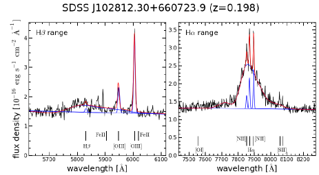
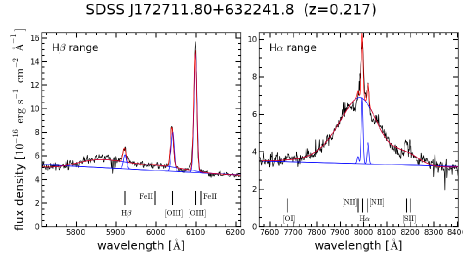
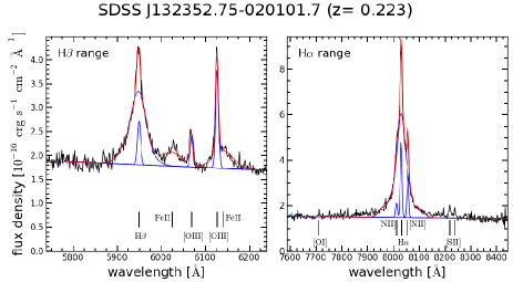
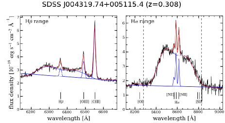
Figure 1.— Observed SDSS spectra (black solid lines) and the corresponding models (red solid lines) in the observed H$\beta$ (left panels) and H$\alpha$ (right panels) wavelength ranges. The fitted individual line components are indicated by blue solid lines (underlying continuum, narrow and broad lines). The most prominent line features are labeled.

We simultaneously model the broad H$\beta$ and H$\alpha$ lines together with the narrow H$\beta$, [O III] $\lambda 4960,\lambda 5007$, H$\alpha$, and [N II] $\lambda 6548,\lambda 6583$ emission lines. We briefly describe our algorithm of modeling the broad H$\alpha$ line below and follow an approach similar to stern_laor_2012. The model of the H$\beta$ region (left panels in Fig. 1) is only used to better constrain the parameters of narrow lines. The well-isolated narrow [O III] line in the H$\beta$ region gives parameter restrictions that are superior to the narrow-line profiles in the H$\alpha$ region, where the narrow and broad lines can be strongly blended.

As a first step, the approximate underlying continua are independently subtracted from the H$\beta$ and H$\alpha$ lines by linear interpolation between the adjacent rest-frame spectral regions 4720–4760 Å and 5070–5130 Å, as well as 6150–6230 Å and 6750–6950 Å, respectively. The fit requires initial guesses for the broad and narrow line components. The initial guesses for the FWHM and line flux of the broad lines are determined by a fourth-order Gauss-Hermite polynomial of the entire H$\alpha$ line and assuming standard H$\alpha$ and H$\beta$ ratios. The initial guesses of the narrow line components are based on the total flux of the observed [O III] line and typical narrow-line AGN ratios. An eighth-order Gauss-Hermite polynomial provides a good fit for the full model of complex broad H$\beta$ and H$\alpha$ line shapes in almost all cases. All narrow emission lines are assumed to have ordinary Gaussian profiles that are coupled in redshift, velocity dispersion, and line ratios for doublets. While [O III] can exhibit a blueshifted wing in cases with an outflow (e.g., mullaney_alexander_2013), the narrow component usually strongly dominates the line flux, and therefore a single-component line fit is generally robust when coupled to lower ionization lines like [N II]. In cases where the outflow component dominates, we decouple [O III] from the fit to other narrow lines, as described below. We also add the two dominant Fe II lines in the H$\beta$ wavelength range as Gaussians to our model. The best-fit model is determined by using a Levenberg–Marquardt minimization algorithm, where spectral regions of unconsidered weak narrow emission lines, e.g., [O I]$\lambda 6300$ and [S II]$\lambda 6718,\lambda 6732$, have been masked out along with pixels assigned as bad by the SDSS spectroscopic pipeline.

We deviate slightly from the scheme above in the following three cases: (1) the broad H$\beta$ line is too weak to be modeled, (2) the [O III] line exceeds a width of 600 km sec^-1, or (3) the narrow H$\alpha$ line flux is negative in the initial best-fit model. In the first case, we repeat the model without any broad H$\beta$ and Fe II components. In the second and third case, the [O III] line is likely to be affected by outflows and may not match the line profile of the other narrow lines. Therefore, we allow the [O III] line to have an independent redshift and velocity dispersion with respect to the other narrow lines.

One percent of the RASS/SDSS spectra do not allow such an analysis because significant parts of the spectral range around H$\alpha$ or [O III] are masked out. We do not expect any significant impact on our study, due to the low number of objects for which this is the case (see also Sect. LABEL:robustness below).

Examples of the best-fit models for typical S/N AGN spectra are shown in Figure 1. From those best-fit models we measure the FWHM and integrated flux of the broad-line H$\alpha$ component, as these are the parameters required to estimate $M_{\rm BH}$ and $L/L_{\rm EDD}$. Our model is not designed to provide a perfect fit to H$\alpha$ line profiles for the most complex cases. However, the model deviations concerning the H$\alpha$ width and flux are much smaller than the systematics of virial $M_{\rm BH}$ estimates (see discussion in denney_peterson_2009). To assess the uncertainties of the derived parameters and to identify unreliable models, we generate 100 realizations of the same spectrum by replacing each pixel within its 1$\sigma$ variance given by the SDSS error spectrum and analyze the artificial spectra in the same manner. The uncertainty for each quantity is then taken as the dispersion (1$\sigma$ error corresponding to 68.3%) in the best-fit value of all 100 measurements.

We compared our measurements with those of stern_laor_2012 to cross-check our results with a completely independent algorithm (Fig. 2) and to provide an estimate of the systematic uncertainties. In contrast to our study, their sample contains lower luminosity AGNs at a slightly different redshift range. Thus, the samples only overlap partially. For the broad H$\alpha$ FWHM and luminosity, we find relatively tight correlations around the unity relation. The measurements of the broad H$\alpha$ FWHM exhibit a larger scatter and are slightly skewed toward lower values using our method. We inspected those spectra and identify a common characteristic in these cases: the narrow lines are broader and weaker than for the other AGNs in the sample. Thus, deblending the narrow [NII]+H$\alpha$ from the broad H$\alpha$ line can be challenging. This is particularly true for broad H$\alpha$ lines with a FWHM less than $4000$ km s^-1. In summary, our line-profile fitting method provides robust estimates for the FWHM and line flux within their systematic uncertainties and without the need for human interaction.

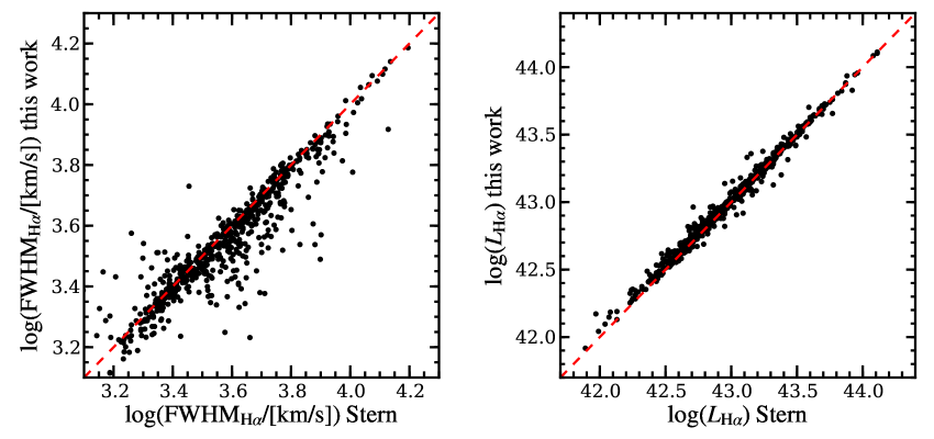
Figure 2.— Comparison of the fitted FWHM and luminosity of the broad H$\alpha$ line component between our work and stern_laor_2012, for sources in both studies. The dashed red lines show the unity correlations. The 1 $\sigma$ scatter about these lines is 0.08 dex (left) and 0.04 dex (right), respectively.

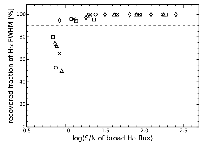
Figure 3.— Accuracy in recovering the FWHM value of the broad H$\alpha$ line as a function of the signal-to-noise ratio (S/N) of the integrated flux of the broad H$\alpha$ line. We use high S/N spectra to simulate 250 realizations at various degraded S/N levels. Within each S/N bin, we determine the fraction of spectra for which the FWHM is within 40% of the original high S/N spectrum (see text for details). We show the results for five different objects indicated by different symbols.

3.2. Estimating $M_{\rm BH}$

The virial black hole mass is estimated by combining the empirically calibrated BLR size-luminosity relation, derived from reverberation mapping monitoring of nearby AGNs, and assuming virialized BLR motions, $M_{\rm BH}=f_{\mathrm{vir}}v^{2}R_{\mathrm{BLR}}G^{-1}$, where $v$ is the FWHM of broad lines in the AGN spectrum and $f_{\mathrm{vir}}$ is the virial factor representing the BLR kinematics. Several different estimators for $M_{\rm BH}$ have independently been reported in the literature using different BLR size-luminosity relations and virial factors based on different assumptions. Here we employ two different calibrations to check their potential impact on our results. The first is from mclure_dunlop_2004:

$$\frac{M_{\mathrm{BH}}}{M_{\sun}}=4.7\left(\frac{L_{5100}}{10^{44}\mathrm{erg}\,\mathrm{s}^{-1}}\right)^{0.61}\left(\frac{\mathrm{FWHM}_{\mathrm{H}\beta}}{\mathrm{km}\,\mathrm{s}^{-1}}\right)^{2}$$ (1)

which is also used by shen_strauss_2009 to estimate $M_{\rm BH}$ for all unobscured, optically selected SDSS AGN. The second calibration is based on the most recent BLR size-luminosity relation of bentz_peterson_2009, assuming a virial factor of $f_{\mathrm{vir}}=5.5$, which is empirically determined by onken_ferrarese_2004:

$$\frac{M_{\mathrm{BH}}}{M_{\sun}}=8.13\left(\frac{L_{5100}}{10^{44}\mathrm{erg}\,\mathrm{s}^{-1}}\right)^{0.52}\left(\frac{\mathrm{FWHM}_{\mathrm{H}\beta}}{\mathrm{km}\,\mathrm{s}^{-1}}\right)^{2}.$$ (2)

Throughout the paper, we use the second calibration (bentz_peterson_2009) for the estimates of the black hole masses. In Sect. LABEL:robustness below we test the robustness of our clustering results if the first calibration method is used instead. As we demonstrate below, we find very similar results using either calibration.

In order to use our measurements from the H$\alpha$ line to estimate $M_{\mathrm{BH}}$, we have to replace $L_{5100}$ by $L_{\rm H\alpha}$ and $\mathrm{FWHM}_{\mathrm{H}\beta}$ by $\mathrm{FWHM}_{\mathrm{H}\alpha}$ in Equations (1) and (2), following greene_ho_2005 (their Equations 1 and 3).

denney_peterson_2009 point out that the inclusion of low S/N spectra adds a systematic offset in $M_{\rm BH}$ estimates because the line width is systematically underestimated. Therefore, we enforce a lower cutoff in the measured S/N level of the broad H$\alpha$ line flux. We determine the cutoff S/N by selecting the five AGN spectra with the highest S/N. Then, we artificially degrade the S/N gradually down to a continuum S/N of 1. For each S/N level, we generate 250 spectra and model these individual spectra with our line-profile fitting method.

At an H$\alpha$ FWHM uncertainty level of greater than 40%, the measurement uncertainties exceed the commonly assumed systematic uncertainties for virial $M_{\mathrm{BH}}$ estimates of $\sim$0.3 dex. More than 90% of all of our generated spectra have FWHM uncertainties of less than 40% if we restrict the H$\alpha$ S/N to values greater than 10 (Figure 3). Consequently, we adapt this S/N threshold as a limit for selecting objects that yield reliable $M_{\mathrm{BH}}$ estimates. This cutoff leads to a removal of 189 out of 1538 objects (12% of the sample). We apply this S/N cut and compare our measured FWHM values to the ones from stern_laor_2012. The observed scatter in FWHM between both methods is 0.08 dex, which corresponds to an $M_{\rm BH}$ error of 0.16. This can be interpreted as a simple estimate of the minimum systematic uncertainty in the $M_{\mathrm{BH}}$ determination, which is reflected in the commonly assumed total $\sim$0.3 dex systematic uncertainty of this method.

The main purpose of this paper is to study the clustering of AGN samples with low and high $M_{\mathrm{BH}}$ and $L/L_{\rm EDD}$, respectively. Any uncertainty in the calibration of $M_{\mathrm{BH}}$ will affect our entire sample similarly. Thus, our results will not depend on the absolute accuracy of the $M_{\mathrm{BH}}$ calibration because we are interested only in relative $M_{\mathrm{BH}}$ values such that we can divide the full sample into low and high $M_{\mathrm{BH}}$ subsamples.

3.3. Estimating $L/L_{\rm EDD}$

The Eddington ratio $L/L_{\rm EDD}$ is the ratio between the bolometric and the Eddington luminosity ($L_{\rm edd}=1.26\times 10^{38}\,M_{\rm BH}/\mathrm{M}_{\odot}$ erg s^-1). The quantity is commonly derived by using the inferred $M_{\rm BH}$ and the optical continuum luminosity at 5100 Å, adopting a certain bolometric correction factor. Different bolometric correction factors used to estimate the bolometric luminosity $L_{\rm bol}$ from $L_{5100}$ are quoted in the literature (kaspi_smith_2000; mclure_dunlop_2004; richards_lacy_2006). While these correction factors are subject to uncertainties, they are required to estimate the bolometric luminosity if only a single-epoch optical spectrum is available. We use a correction factor of $f=10.3$ (richards_lacy_2006), which is consistent with values used by other studies. Again, we use the relation from greene_ho_2005 to estimate $L_{5100}$ from $L_{\rm H\alpha}$ for the computation of $L_{\rm bol}$.

3.4. Defining X-ray Selected AGN Subsamples

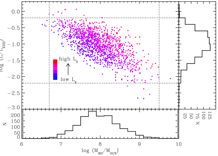
Figure 4.— $M_{\rm BH}$ vs. $L/L_{\rm EDD}$ for luminous, unabsorbed, broad-line, X-ray selected RASS/SDSS AGNs with a broad H$\alpha$ luminosity of $S/N>10$. The color of the symbols encodes the X-ray luminosity of the sources. The lower and right panels show histograms of $M_{\rm BH}$ and $L/L_{\rm EDD}$, respectively, for the full sample. The dotted lines mark the restriction of the parameter space in our analysis to remove extreme objects.

The RASS/SDSS AGNs in our sample do not uniformly populate the $M_{\rm BH}$ – $L/L_{\rm EDD}$ plane (Figure 4). Although there is substantial scatter, on average, higher $L/L_{\rm EDD}$ are found in AGNs with lower $M_{\rm BH}$. While the absence of objects in the upper right corner of this plane is not an observational bias, but reflects the nonexistence of (unabsorbed) RASS/SDSS AGNs with both high $M_{\rm BH}$ and high $L/L_{\rm EDD}$ in the redshift range studied here, the lack of objects in the lower left corner reflects an observational bias. AGNs with low $L/L_{\rm EDD}$ and low $M_{\rm BH}$ are too weak to produce a significant broad H$\alpha$ line relative to the host galaxy continuum. The H$\alpha$ flux S/N cutoff used here primarily removes objects with log ($M_{\rm BH}$/$M_{\odot}$) $\sim$ 7–8.

Since $M_{\rm BH}$ and $L/L_{\rm EDD}$ are correlated in our full sample, and we aim to reveal which of these quantities drives the observed X-ray luminosity dependence of AGN clustering, doing a simple cut of the full sample into low and high $M_{\rm BH}$ subsamples, as well as high and low $L/L_{\rm EDD}$ subsamples, will not be useful. When creating subsamples that depend on one parameter, the distribution of the second parameter in both subsamples must be the same. This “matching” of the subsamples is a commonly used method in clustering measurements (e.g., coil_georgakakis_2009). However, one has to test that the procedure of creating matched subsamples is not introducing a bias to the clustering results. We will do so below by testing different methods to produce matched subsamples (see Sect. LABEL:robustness).

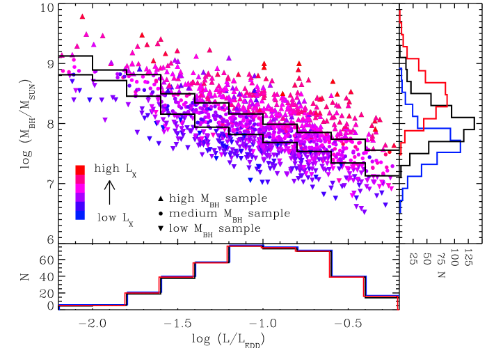
Figure 5.— Low (filled down-pointing triangles), medium (filled circles), and high (filled up-pointing triangles) $M_{\rm BH}$ RASS/SDSS AGN subsamples with matched $L/L_{\rm EDD}$ distributions. The top panel shows the $L/L_{\rm EDD}$–$M_{\rm BH}$ plane. The color of the points encodes the X-ray luminosity from lowest $L_{\rm X}$ (blue) to highest $L_{\rm X}$ (red). The solid lines are for visual guidance and mark the division of the full AGN sample into low, medium, and high $M_{\rm BH}$ subsamples. The bottom and right panels show the $L/L_{\rm EDD}$ and $M_{\rm BH}$ histograms of the low (blue), medium (black), and high (red) $M_{\rm BH}$ subsamples, respectively. Since the medium $M_{\rm BH}$ subsample contains more objects than the low and high subsamples, we normalized the total number of this sample in the $L/L_{\rm EDD}$ histogram to match the other samples. For clarity, we slightly shift the $x$ values of the low and high $M_{\rm BH}$ subsamples in the histograms.

Before creating low and high $M_{\rm BH}$ subsamples, objects that lie outside the range $-2.2<{\rm log}(L/L_{\rm EDD})<-0.2$ are removed. We then determine the number of objects in each $L/L_{\rm EDD}$ bin, using a bin width of 0.2 (logarithmic scale). In each $L/L_{\rm EDD}$ bin, we create three subsamples: 30% of objects with the lowest $M_{\rm BH}$, 40% with medium $M_{\rm BH}$, and 30% of objects with the highest $M_{\rm BH}$ (Figure 5). The procedure creates low, medium, and high $M_{\rm BH}$ AGN subsamples with extremely similar (“matched”) $L/L_{\rm EDD}$ distributions but different median $M_{\rm BH}$ (see Table 5). All $M_{\rm BH}$ AGN subsamples have median $\langle{\rm log}\,(L/L_{\rm EDD})\rangle=-1.00$.

The low (30%), medium (40%), and high (30%) $L/L_{\rm EDD}$ RASS/SDSS AGN subsamples with matched $M_{\rm BH}$ distributions are created by first applying a cut of $6.7<{\rm log}(M_{\rm BH}/M_{\odot})<9.5$ to remove extreme sources and then following the same approach as described above, using bins of $M_{\rm BH}$ with a bin width of 0.2 (logarithmic scale). All $L/L_{\rm EDD}$ AGN subsamples have median $\langle$log ($M_{\rm BM}$/$M_{\odot}$)$\rangle=7.92-7.93$.

Figures 4 and 5 show that divisions into low, medium, and high $M_{\rm BH}$ as well as $L/L_{\rm EDD}$ are very similar to divisions into low, medium, and high $L_{\rm X}$. Thus, one cannot anticipate if the X-ray luminosity clustering dependence is related to $L/L_{\rm EDD}$ or $M_{\rm BH}$, as we aim to test here.

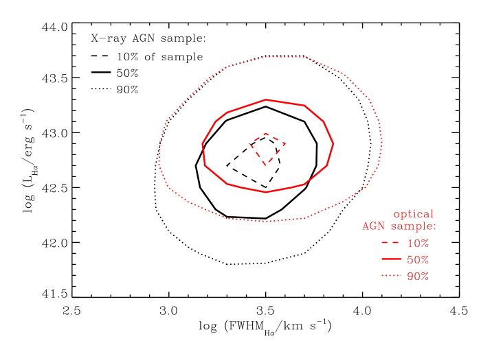
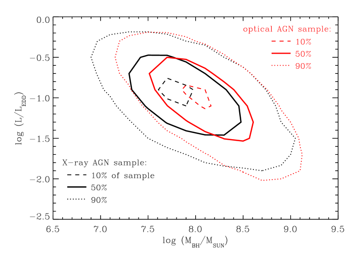
Figure 6.— Comparison between the X-ray-selected RASS/SDSS AGNs (black lines) and the optically selected SDSS AGN samples (red lines). The contours show the location of 10% (dashed lines), 50% (solid lines), and 90% (dotted line) of the full sample, respectively. The left figure shows the observed parameters, luminosity and FWHM of the H$\alpha$ line, while the right figure shows the derived parameters $L/L_{\rm EDD}$ and $M_{\rm BH}$. In both figures, a boxcar smoothing with a width of two has been applied.

The directly observed parameters FWHM and $L_{\rm H\alpha}$ do not correlate with each other as strongly as $M_{\rm BH}$ and $L/L_{\rm EDD}$ (see Fig. 6). However, we decide to use the same method to create subsamples defined by FWHM and $L_{\rm H\alpha}$ as well. Thus, we again split the full sample into three subsamples defined using one parameter, while maintaining the same distribution in the other parameter of interest. To create subsamples in FWHM, we first limit to objects with $41.7<{\rm log}(L_{\rm H\alpha}/[$erg s${}^{-1}])<44.1$ and then use a bin width of 0.2. All FWHM AGN subsamples have $\langle{\rm log}(L_{\rm H\alpha}/[$erg s${}^{-1}])\rangle=42.72-42.73$. To create subsamples in $L_{\rm H\alpha}$, we first limit to objects with $2.9<{\rm log}(\rm FWHM/[$km s${}^{-1}])<4.1$, and then use bins of width 0.1, using the logarithmic values of FWHM. This choice of bin width ensures a similar numbers of bins as compared to the subsamples defined in $L_{\rm H\alpha}$. The median FWHM of all $L_{\rm H\alpha}$ subsamples is $\langle{\rm FWHM}\rangle=2850-2960$ km s^-1.

As we have to exclude $\sim$13% of the RASS/SDSS AGN sample studied in Papers I–III to fulfill our S/N requirement of the broad H$\alpha$ line flux for reliable $M_{\rm BH}$ estimates, we create low and high X-ray luminosity subsamples of the reduced AGN sample used here. We use a simple 0.1-2.4 keV luminosity cut (with no matching of the distribution of another parameter) of log $(L_{\rm X}/[$erg s${}^{-1}])=44.29$, identical to that used in Papers I–III.

We also apply simple $M_{i}$ cuts at $M_{i}=-22.10$ mag and $M_{i}=-22.70$ mag to divide the X-ray-selected AGN sample into a faint (33% of all objects), medium (34%), and luminous (33%) $M_{i}$ subsamples. Finally, we compute from the SDSS optical spectra the rest-frame absolute magnitude in the band between 5500 and 6800 Å, which includes the H$\alpha$ line for all objects. We do this as the X-ray and optically selected sample covers a redshift range of $0.16<z<0.36$, while the H$\alpha$ line is redshifted outside the SDSS $i$-band filter above $z\sim 0.28$. The division into three subsamples of similar size is realized by applying cuts at $M_{5500-6800}^{\rm rest}=-21.72$ mag and $M_{5500-6800}^{\rm rest}=-22.33$ mag. We do not match the distribution of any other parameter for these subsamples. All samples used in this paper are presented in Table 5.

3.5. Defining the Optically Selected AGN Subsamples

The optically selected SDSS AGNs (called “quasars” in the SDSS literature) are drawn from the catalog provided by schneider_richards_2010. Instead of using the classic selection in the $B$-band, schneider_richards_2010 use the SDSS $i$-band, as it is less affected by Galactic absorption. However, this comes with the significant disadvantage that host-galaxy light might represent a significant fraction of the total flux in the $i$-filter. schneider_richards_2010 apply an apparent magnitude cut of $M_{\rm i}\leq-22$ and require that objects have at least one emission line exceeding an FWHM of 1000 km s^-1. Unlike our RASS/SDSS AGN sample, this sample of 3500 objects ($0.16\leq z\leq 0.36$) has the footprint of SDSS Data Release 7. The DR4+ and DR7 areas are 5468 deg² and 7670 deg², respectively, when we consider only the area that has a DR7 completeness ratio of $f_{\rm compl}>0.8$. Thus the area occupied by the optically selected AGN sample is 1.4 times larger than the area covered by the X-ray-selected AGN sample. Additionally, the number density (per square degree) of optically selected AGNs is 1.6 times higher than for the X-ray-selected AGNs.

We retrieve the individual SDSS spectra of the optically selected SDSS AGNs and derive the FWHM of the broad H$\alpha$ line and the $L_{\rm H\alpha}$ through spectral fits (see Sect. 3). This procedure is identical to the one used for the RASS/SDSS AGN sample (see Sect. 3.1). We select only objects with $S/N>10$ in the flux of the broad H$\alpha$ line. We derive the individual black hole masses and $L/L_{\rm EDD}$ for the remaining 2831 AGNs. The X-ray and optically selected AGN samples have 807 objects in common, which is 29% of the total optically selected AGN sample. Thus, there is substantial difference between the X-ray and optically selected AGN samples.

Figure 6 compares how the X-ray-selected RASS/SDSS AGN sample and the optically selected SDSS AGN sample span the observed parameter space of $L_{\rm H\alpha}$ and FWHM (left panel) and the derived parameter space of $L/L_{\rm EDD}$ and $M_{\rm BH}$ (right panel). In the observed parameter space, there are two obvious differences between these samples. First, the RASS/SDSS AGN sample extends to lower $L_{\rm H\alpha}$. This is likely a consequence of rejecting AGNs with $M_{\rm i}>-22$ in order to exclude objects with a strong starlight component from the host galaxy because an AGN has to have a certain luminosity to outshine its host galaxy. Clearly, X-ray selection of AGNs (RASS/SDSS) allows us to extend to fainter AGN luminosities, below the optical cut. Thus, at X-ray wavelengths we are able to detect AGNs that might not outshine their host galaxy in the optical (see, e.g., hopkins_hickox_2009). At log ($L_{\rm H\alpha}/[{\rm erg}\,{\rm s}^{-1}])\,>42.5$, both samples span a similar parameter space, and the dynamic range in FWHM is almost identical in both samples.

Differences in the observed parameter space naturally translate into differences in the derived $M_{\rm BH}$–$L/L_{\rm EDD}$ space (Fig. 6, right panel). Compared with the X-ray-selected AGN sample, the optical AGN sample has a deficiency of AGNs with low $M_{\rm BH}$. The optically selected sample also extends marginally to higher $M_{\rm BH}$ and lower $L/L_{\rm EDD}$.

We create optically selected AGN subsamples with respect to $M_{\rm BH}$, $L/L_{\rm EDD}$, FWHM, and $L_{\rm H\alpha}$ (with matched distribution in the other parameter of interest; see Sect. 3.4). We have to use slightly different limits for some of the parameters because the X-ray and optically selected AGN samples cover slightly different parameter spaces. Thus, when we create the low, medium, and high $M_{\rm BH}$ subsamples with matched $L/L_{\rm EDD}$ distributions, we use an $L/L_{\rm EDD}$ limit of $-2.3<{\rm log}(L/L_{\rm EDD})<0.1$. The optical $M_{\rm BH}$ subsamples have median $\langle{\rm log}\,(L/L_{\rm EDD})\rangle=-1.04$ to $-1.00$, while the $L/L_{\rm EDD}$ subsamples have $\langle$log ($M_{\rm BM}$/$M_{\odot}$)$\rangle=8.12-8.13$.

When we create three subsamples in FWHM, we limit $L_{\rm H\alpha}$ to $42.1<{\rm log}(L_{\rm H\alpha}/[$erg s${}^{-1}])<44.1$. The FWHM subsamples have $\langle{\rm log}(L_{\rm H\alpha}/[$erg s${}^{-1}])\rangle=42.88$. For the $L_{\rm H\alpha}$ subsamples, we apply a limit of $2.8<{\rm log}(\rm FWHM/[$km s${}^{-1}])<4.2$. We find $\langle{\rm FWHM}\rangle=3240-3280$ km s^-1 for the low, medium, and high $L_{\rm H\alpha}$ subsamples. All bin widths are identical to the ones used for defining the X-ray-selected AGN subsamples.

We produce optical AGN subsamples divided by $M_{\rm i}$. We use simple $M_{\rm i}$ cuts of $M_{\rm i}=-22.27$ and $M_{\rm i}=-22.67$ to construct faint, medium, and luminous $M_{\rm i}$ subsamples with similar numbers of sources. Finally, we create $M_{5500-6800}^{\rm rest}$ subsamples of the optically selected AGN. We use cuts at $M_{5500-6800}^{\rm rest}=-22.13$ mag and $M_{5500-6800}^{\rm rest}=-22.53$ mag. As with the X-ray-selected AGNs, we do not match the distribution of any other parameter when creating the subsamples defined by $M_{\rm i}$ and $M_{5500-6800}^{\rm rest}$. All samples are presented in Table 5.

4. Methodology

4.1. Clustering Measurements

We measure the two-point correlation function $\xi(r)$ (peebles_1980), which measures the excess probability $dP$ above a Poisson distribution of finding an object in a volume element $dV$ at a distance $r$ from another randomly chosen object. The ACF measures the spatial clustering of objects in the same sample, while the CCF measures the clustering of objects in two different samples. We use the same approach as described in detail in Section 3 of Paper I and Section 4 in Paper III. Here we explain the essential elements of our method.

We use the correlation estimator of davis_peebles_1983 in the form

$$\xi(r)=\frac{DD(r)}{DR(r)}-1\ ,$$ (3)

where $DD(r)$ is the number of data–data pairs with a separation $r$, and $DR(r)$ is the number of data–random pairs. Both pair counts have been normalized by the number density of data and random points. To separate the effect of redshift distortions, the correlation function is measured as a function of two components of the separation vector between two objects, that is, one perpendicular to ($r_{p}$) and the other along ($\pi$) the line of sight. The parameter $\xi(r_{p},\pi)$ is thus extracted by counting pairs on a two-dimensional grid of separations $r_{p}$ and $\pi$. We obtain the projected correlation function $w_{p}(r_{p})$ by integrating $\xi(r_{p},\pi)$ along the $\pi$ direction.

As in Paper I, we infer the AGN ACF from the CCF between AGN and the corresponding galaxy tracer set and the ACF of the tracer set following coil_georgakakis_2009:

$$w_{p}({\rm AGN}|{\rm AGN})=\frac{\left[w_{p}({\rm AGN}|{\rm trace})\right]^{2}}{w_{p}({\rm trace}|{\rm trace})}\,,$$ (4)

where $w_{p}({\rm AGN}|{\rm AGN})$ and $w_{p}({\rm trace}|{\rm trace})$ are the ACFs of the AGN and the corresponding tracer set, respectively, and $w_{p}({\rm AGN}|{\rm trace})$ is the CCF between the AGN and the tracer set (i.e., a galaxy sample).

The CCF is computed using

$$\xi_{\rm AGN-trace}=\frac{D_{\rm AGN}\,D_{\rm trace}}{D_{\rm AGN}\,R_{\rm trace}}-1.$$ (5)

For our purposes, the use of this simple estimator has several major advantages and results in only a marginal loss in the S/N when compared to more advanced estimators (e.g., landy_szalay_1993). The estimator in Equation (5) requires the generation of a random catalog only for the tracer set. Since the random catalog should exactly match all observational biases to minimize the systematic uncertainties, well-understood selection effects are key to creating proper random samples. The tracer sets have well-defined selection functions, while the AGN samples suffer from selection functions that are very complex and difficult to model.

4.2. Error Analysis

The measurements in the adjacent bins of the correlation function are not independent. Poisson errors will significantly underestimate the uncertainties and should not be used for error calculations. Instead, we use the jackknife resampling technique to estimate the measurement errors based on the covariance matrix $M_{ij}$, which reflects the degree to which bin $i$ is correlated with bin $j$.

In our jackknife resampling, we divide the survey area into $N_{\rm T}=100$ subsections for the DR4+ geometry (X-ray-selected AGN sample), each of which is $\sim$50–60 deg². Since the optically selected AGN sample uses the DR7 geometry, we divide this area into $N_{\rm T}=131$ subsections of roughly equal area. These $N_{\rm T}$ jackknife-resampled correlation functions define the covariance matrix:

$$M_{ij}=\frac{N_{\rm T}-1}{N_{\rm T}}\left[\sum_{k=1}^{N_{\rm T}}\bigg{(}w_{k}(r_{p,i})-<w(r_{p,i})>\bigg{)}\right.$$

$$\times\bigg{(}w_{k}(r_{p,j})-<w(r_{p,j})>\bigg{)}\bigg{]}\,$$ (6)

We calculate $w_{p}(r_{p})$ $N_{\rm T}$ times, where each jackknife sample excludes one section and $w_{k}(r_{p,i})$ and $w_{k}(r_{p,j})$ are from the $k$th jackknife samples of the AGN ACF and $<w(r_{p,i})>$, $<w(r_{p,j})>$ are the averages over all of the jackknife samples. The uncertainties represent 1$\sigma$ (68.3%) confidence intervals.

The generation of the covariance matrix for the inferred AGN ACF considers the $N_{\rm T}$ jackknife-resampled correlation functions of the CCF (AGN and corresponding tracer set) and the tracer set ACF. For each jackknife sample, we calculate the inferred AGN ACF by using Equation 4. The resulting $N_{\rm T}$ $w_{p}(r_{p})$ jackknife-resampled projected correlation functions of the inferred ACFs are then used to compute the covariance matrix of the inferred AGN ACF.

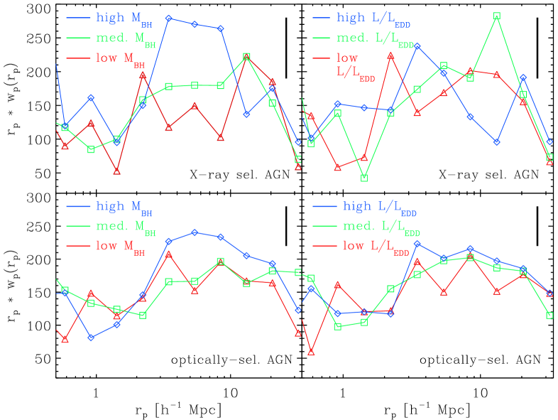
Figure 7.— Directly measured cross-correlation functions between AGN subsamples for different parameters with matched distributions in the other parameter of interest. In the top row we show the results for the X-ray-selected AGNs, while the bottom row shows results for the optically selected AGNs. In each panel, the color encodes the low (red), medium (green), and high (blue) subsample in the corresponding parameter. For the sake of clarity, we show only a typical error bar in each panel (black solid vertical line in right upper corner of each panel). Note that we show on the $y$ axis $r_{\rm p}\times w(r_{\rm p})$ instead of $w(r_{\rm p})$ to allow for an easier comparison between the different subsamples and to make the values easier to read in the figure.

5. Results

We measure high-accuracy CCFs of the different AGN samples with the LRG tracer set (see Fig. 7). In addition, we compute the high-precision ACF of the LRG sample. In both cases, we measure $r_{p}$ in the range 0.05–40 $h^{-1}$ Mpc in 15 logarithmic bins, identical to those used in Paper III. We compute $\pi$ in steps of 5 $h^{-1}$ Mpc in the range $\pi=0-200$ $h^{-1}$ Mpc.

To derive $\pi_{\rm max}$, we compute $w_{p}(r_{p})$ for a set of $\pi_{\rm max}$ ranging from 10 to 160 $h^{-1}$ Mpc in steps of 10 $h^{-1}$ Mpc. We then fit $w_{p}(r_{p})$ over an $r_{p}$ range of 0.3–40 $h^{-1}$ Mpc with a fixed $\gamma=1.9$ and determine the correlation length $r_{\rm 0}$ for the individual $\pi_{\rm max}$ measurements. As in Papers I–III, we find that the LRG ACF saturates at $\pi_{\rm max}=80$ $h^{-1}$ Mpc. All CCFs saturate at $\pi_{\rm max}=40$ $h^{-1}$ Mpc. Power-law fits for the ACFs and CCFs are based on

$$w_{p}(r_{p}) = r_{p}\left(\frac{r_{\rm 0}}{r_{p}}\right)^{\gamma}\,\frac{\Gamma(1/2)\Gamma((\gamma-1)/2)}{\Gamma(\gamma/2)},$$ (7)

where $\Gamma(x)$ is the Gamma function.

To derive the clustering properties of the AGN samples, we follow two different approaches:

(1) Power-law fits to the inferred AGN ACF:
We use Eq. 4 to infer the ACF for the individual AGN sample from the CCF of this sample with the LRG tracer set and the ACF of the LRG sample. We fit the data points of the inferred AGN ACFs with the expression given in Eq. 7 and derive best-fit $r_{\rm 0}$ and $\gamma$ values. The data are fitted over the range $r_{p}=0.3-15$ $h^{-1}$ Mpc to be consistent with Papers I–III. Since we measure the CCF to infer the ACF, the resulting effective redshift distribution for the clustering signal is determined by both the redshift distribution of the tracer set and the AGN sample: $N_{\rm CCF}(z)=N_{\rm tracer}(z)*N_{\rm AGN}(z)$.

In Table 5 we list the redshift range, the median effective redshift of $N_{\rm CCF}(z)$ for the corresponding AGN samples, the derived best $r_{\rm 0}$ and $\gamma$ values based on power-law fits, and $r_{\rm 0}$ for a power-law fit with a fixed slope of $\gamma=1.9$ (for ease of comparison).

(2) Bias from HOD modeling: In Paper II we develop a novel method to infer the HOD of RASS/SDSS AGNs directly from the well-constrained CCF of RASS/SDSS AGNs with LRGs. In performing the HOD modeling, we consider that galaxies and AGNs are associated with DMHs. A DMH may contain one or more galaxies or AGNs that are included in our samples. Using the HOD of the LRGs as a template, we constrain the HOD of the AGN by fitting the CCF between AGNs and LRGs. A few of the CCFs do not have enough pairs on small scales for applying $\chi^{2}$ statistics. Thus to derive consistent constraints for all CCF, we consider only bins with $r_{\rm p}>0.7$ $h^{-1}$ Mpc for all CCF fits (as in Paper III).

Table 1Properties of Inferred AGN ACFs and Derived Quantities

AGN Sample	Number	Median	10th,50th,90th	$r_{\rm 0}$	$\gamma$	$r_{\rm 0,\gamma=1.9}$	$b(z)$	log $M_{\rm DMH}^{\rm typ}$
Name	of Objects	$z_{\rm eff}$	Percentile	($h^{-1}$ Mpc)		($h^{-1}$ Mpc)	HOD	($h^{-1}$ $M_{\odot}$)
X-ray Selected AGN — RASS/SDSS AGN — SDSS Data Release 4+
total RASS AGN	1349	0.27	43.70,44.17,44.68	4.02${}^{+0.45}_{-0.57}$	1.62${}^{+0.15}_{-0.14}$	4.09${}^{+0.35}_{-0.39}$	1.32${}^{+0.11}_{-0.09}$	13.20${}^{+0.13}_{-0.13}$
low $L_{\rm X}$ RASS	858	0.25	43.63,43.99,44.23	3.12${}^{+0.57}_{-0.89}$	1.55${}^{+0.25}_{-0.21}$	3.28${}^{+0.41}_{-0.46}$	1.22${}^{+0.14}_{-0.12}$	13.08${}^{+0.19}_{-0.20}$
high $L_{\rm X}$ RASS	491	0.29	44.34,44.53,44.87	5.38${}^{+0.68}_{-0.87}$	1.88${}^{+0.18}_{-0.18}$	5.41${}^{+0.65}_{-0.73}$	1.53${}^{+0.15}_{-0.17}$	13.41${}^{+0.13}_{-0.18}$
low $M_{\rm BM}$ RASS	410	0.22	7.07,7.54,8.01	2.71${}^{+0.53}_{-1.11}$	2.07${}^{+1.46}_{-0.64}$	2.65${}^{+0.56}_{-0.71}$	0.96${}^{+0.24}_{-0.12}$	12.60${}^{+0.48}_{-0.39}$
medium $M_{\rm BM}$ RASS	525	0.27	7.55,7.92,8.36	4.34${}^{+0.64}_{-0.90}$	1.61${}^{+0.19}_{-0.18}$	4.32${}^{+0.52}_{-0.58}$	1.38${}^{+0.15}_{-0.17}$	13.27${}^{+0.16}_{-0.23}$
high $M_{\rm BM}$ RASS	400	0.29	7.92,8.38,8.91	4.60${}^{+0.82}_{-1.11}$	1.85${}^{+0.21}_{-0.22}$	4.67${}^{+0.78}_{-0.92}$	1.62${}^{+0.20}_{-0.16}$	13.49${}^{+0.16}_{-0.15}$
low $L/L_{\rm EDD}$ RASS	418	0.23	-1.79,-1.36,-0.98	3.00${}^{+0.78}_{-1.20}$	1.45${}^{+0.26}_{-0.21}$	3.17${}^{+0.54}_{-0.64}$	1.30${}^{+0.18}_{-0.18}$	13.21${}^{+0.21}_{-0.27}$
medium $L/L_{\rm EDD}$ RASS	522	0.27	-1.36,-1.00,-0.71	2.87${}^{+1.97}_{-1.50}$	1.59${}^{+0.40}_{-0.33}$	2.89${}^{+0.46}_{-0.54}$	1.29${}^{+0.13}_{-0.15}$	13.16${}^{+0.16}_{-0.23}$
high $L/L_{\rm EDD}$ RASS	404	0.29	-1.01,-0.68,-0.35	4.36${}^{+0.67}_{-0.79}$	2.14${}^{+0.22}_{-0.19}$	3.92${}^{+0.74}_{-0.89}$	1.18${}^{+0.15}_{-0.14}$	12.97${}^{+0.22}_{-0.26}$
low FWHM RASS	415	0.27	1280,1910,2470	2.69${}^{+0.61}_{-0.80}$	2.30${}^{+0.72}_{-0.40}$	$2.32^{+0.71}_{-1.01}$	1.09${}^{+0.12}_{-0.12}$	12.84${}^{+0.20}_{-0.27}$
medium FWHM RASS	525	0.26	2340,2890,3690	2.90${}^{+1.25}_{-2.35}$	1.35${}^{+0.24}_{-0.28}$	$3.70^{+0.64}_{-0.76}$	1.47${}^{+0.17}_{-0.18}$	13.38${}^{+0.16}_{-0.21}$
high FWHM RASS	404	0.27	3650,4840,7920	3.52${}^{+0.92}_{-1.57}$	1.53${}^{+0.25}_{-0.26}$	$3.82^{+0.65}_{-0.77}$	1.53${}^{+0.17}_{-0.18}$	13.43${}^{+0.15}_{-0.20}$
low $L_{\rm H\alpha}$ RASS	414	0.22	41.99,42.29,42.53	2.14${}^{+0.96}_{-1.72}$	1.39${}^{+0.56}_{-0.32}$	2.69${}^{+0.54}_{-0.66}$	1.21${}^{+0.18}_{-0.19}$	13.10${}^{+0.23}_{-0.35}$
medium $L_{\rm H\alpha}$ RASS	526	0.27	42.52,42.74,42.96	1.96${}^{+1.00}_{-1.97}$	1.83${}^{+1.32}_{-0.36}$	2.13${}^{+0.64}_{-0.71}$	1.31${}^{+0.16}_{-0.16}$	13.18${}^{+0.19}_{-0.24}$
high $L_{\rm H\alpha}$ RASS	403	0.29	42.93,43.22,43.63	3.52${}^{+0.92}_{-1.57}$	1.53${}^{+0.25}_{-0.26}$	3.82${}^{+0.65}_{-0.78}$	1.36${}^{+0.18}_{-0.16}$	13.23${}^{+0.19}_{-0.23}$
faint $M_{i}$ RASS	444	0.23	-21.26,-21.80,-22.04	3.21${}^{+0.69}_{-1.58}$	1.69${}^{+0.69}_{-0.42}$	$3.32^{+0.58}_{-0.70}$	1.10${}^{+0.26}_{-0.14}$	12.90${}^{+0.39}_{-0.31}$
medium $M_{i}$ RASS	460	0.27	-22.15,-22.39,-22.63	3.51${}^{+0.71}_{-1.16}$	1.71${}^{+0.36}_{-0.29}$	$3.65^{+0.61}_{-0.72}$	1.21${}^{+0.19}_{-0.16}$	13.04${}^{+0.25}_{-0.29}$
luminous $M_{i}$ RASS	445	0.29	-22.76,-23.13,-23.96	3.04${}^{+0.76}_{-1.12}$	1.47${}^{+0.17}_{-0.18}$	2.94${}^{+0.54}_{-0.65}$	1.48${}^{+0.17}_{-0.16}$	13.36${}^{+0.16}_{-0.19}$
faint $M_{5500-6800}^{\rm rest}$ RASS	444	0.22	-20.84,-21.39,-21.66	3.18${}^{+0.63}_{-1.12}$	1.79${}^{+0.56}_{-0.41}$	$3.19^{+0.59}_{-0.71}$	1.13${}^{+0.25}_{-0.19}$	12.97${}^{+0.35}_{-0.42}$
med. $M_{5500-6800}^{\rm rest}$ RASS	460	0.27	-21.79,-22.02,-22.27	2.44${}^{+1.15}_{-1.94}$	1.36${}^{+0.29}_{-0.28}$	$3.39^{+0.57}_{-0.67}$	1.25${}^{+0.16}_{-0.17}$	13.10${}^{+0.20}_{-0.28}$
lum. $M_{5500-6800}^{\rm rest}$ RASS	445	0.30	-22.42,-22.81,-23.67	4.23${}^{+0.76}_{-1.00}$	1.70${}^{+0.15}_{-0.16}$	4.20${}^{+0.67}_{-0.79}$	1.44${}^{+0.16}_{-0.17}$	13.31${}^{+0.15}_{-0.21}$
Optically Selected AGN — SDSS AGN — SDSS Data Release 7
total SDSS AGN	2831	0.29	-22.08,-22.45,-23.34	5.07${}^{+0.26}_{-0.28}$	1.80${}^{+0.09}_{-0.09}$	5.06${}^{+0.25}_{-0.26}$	1.32${}^{+0.07}_{-0.06}$	13.18${}^{+0.08}_{-0.09}$
faint $M_{i}$ SDSS	932	0.28	-22.03,-22.13,-22.24	5.34${}^{+0.42}_{-0.51}$	1.80${}^{+0.20}_{-0.19}$	5.34${}^{+0.40}_{-0.43}$	1.47${}^{+0.09}_{-0.14}$	13.36${}^{+0.09}_{-0.16}$
medium $M_{i}$ SDSS	966	0.29	-22.30,-22.45,-22.63	3.79${}^{+0.44}_{-0.59}$	1.73${}^{+0.16}_{-0.16}$	3.97${}^{+0.36}_{-0.39}$	1.20${}^{+0.09}_{-0.10}$	13.00${}^{+0.14}_{-0.17}$
luminous $M_{i}$ SDSS	933	0.30	-22.73,-23.06,-23.86	4.48${}^{+0.51}_{-0.64}$	1.63${}^{+0.12}_{-0.12}$	4.52${}^{+0.41}_{-0.45}$	1.40${}^{+0.12}_{-0.12}$	13.26${}^{+0.13}_{-0.15}$
low $M_{\rm BM}$ SDSS	857	0.27	7.37,7.82,8.35	4.24${}^{+0.46}_{-0.56}$	1.74${}^{+0.15}_{-0.15}$	4.26${}^{+0.41}_{-0.45}$	1.28${}^{+0.12}_{-0.13}$	13.14${}^{+0.15}_{-0.20}$
medium $M_{\rm BM}$ SDSS	1114	0.30	7.70,8.08,8.59	4.97${}^{+0.40}_{-0.48}$	1.98${}^{+0.17}_{-0.18}$	4.88${}^{+0.41}_{-0.44}$	1.18${}^{+0.13}_{-0.09}$	12.96${}^{+0.19}_{-0.16}$
high $M_{\rm BM}$ SDSS	845	0.31	8.04,8.45,8.97	4.72${}^{+0.63}_{-0.82}$	1.50${}^{+0.12}_{-0.12}$	4.76${}^{+0.43}_{-0.47}$	1.60${}^{+0.10}_{-0.08}$	13.45${}^{+0.09}_{-0.07}$
low $L/L_{\rm EDD}$ SDSS	859	0.28	-1.84,-1.31,-0.88	3.40${}^{+0.55}_{-0.77}$	1.58${}^{+0.14}_{-0.15}$	3.62${}^{+0.39}_{-0.44}$	1.21${}^{+0.11}_{-0.10}$	13.03${}^{+0.16}_{-0.17}$
medium $L/L_{\rm EDD}$ SDSS	1113	0.30	-1.53,-1.04,-0.67	4.68${}^{+0.58}_{-0.73}$	1.62${}^{+0.13}_{-0.13}$	4.89${}^{+0.43}_{-0.46}$	1.40${}^{+0.11}_{-0.11}$	13.26${}^{+0.12}_{-0.14}$
high $L/L_{\rm EDD}$ SDSS	845	0.31	-1.17,-0.74,-0.40	4.75${}^{+0.60}_{-0.78}$	1.64${}^{+0.14}_{-0.15}$	4.73${}^{+0.50}_{-0.55}$	1.49${}^{+0.15}_{-0.12}$	13.35${}^{+0.14}_{-0.13}$
low FWHM SDSS	857	0.30	1490,2110,2560	4.18${}^{+0.49}_{-0.56}$	1.92${}^{+0.19}_{-0.19}$	$4.17^{+0.49}_{-0.55}$	1.11${}^{+0.13}_{-0.08}$	12.84${}^{+0.21}_{-0.17}$
medium FWHM SDSS	1120	0.29	2680,3260,4040	5.03${}^{+0.43}_{-0.53}$	1.75${}^{+0.13}_{-0.13}$	$5.12^{+0.38}_{-0.40}$	1.41${}^{+0.10}_{-0.09}$	13.28${}^{+0.11}_{-0.11}$
high FWHM SDSS	847	0.29	4300,5500,8460	4.62${}^{+0.50}_{-0.63}$	1.68${}^{+0.14}_{-0.14}$	4.71${}^{+0.42}_{-0.46}$	1.44${}^{+0.10}_{-0.12}$	13.32${}^{+0.10}_{-0.15}$
low $L_{\rm H\alpha}$ SDSS	859	0.27	42.40,42.61,42.71	3.72${}^{+0.51}_{-0.72}$	1.63${}^{+0.16}_{-0.17}$	3.79${}^{+0.41}_{-0.45}$	1.25${}^{+0.13}_{-0.08}$	13.10${}^{+0.17}_{-0.12}$
medium $L_{\rm H\alpha}$ SDSS	1119	0.30	42.76,42.89,43.04	4.25${}^{+0.49}_{-0.68}$	1.69${}^{+0.15}_{-0.16}$	4.47${}^{+0.39}_{-0.42}$	1.32${}^{+0.12}_{-0.10}$	13.16${}^{+0.15}_{-0.14}$
high $L_{\rm H\alpha}$ SDSS	846	0.31	43.07,43.26,43.63	4.52${}^{+0.61}_{-0.80}$	1.56${}^{+0.14}_{-0.14}$	4.50${}^{+0.46}_{-0.51}$	1.52${}^{+0.13}_{-0.13}$	13.38${}^{+0.12}_{-0.14}$
faint $M_{5500-6800}^{\rm rest}$ SDSS	933	0.27	-21.70,-21.97,-22.10	5.96${}^{+0.41}_{-0.44}$	1.88${}^{+0.13}_{-0.14}$	$5.95^{+0.40}_{-0.43}$	1.50${}^{+0.09}_{-0.14}$	13.40${}^{+0.09}_{-0.15}$
med. $M_{5500-6800}^{\rm rest}$ SDSS	964	0.30	-22.17,-22.31,-22.49	3.36${}^{+0.71}_{-1.18}$	1.55${}^{+0.20}_{-0.22}$	$3.96^{+0.40}_{-0.45}$	1.14${}^{+0.10}_{-0.11}$	12.89${}^{+0.16}_{-0.22}$
lum. $M_{5500-6800}^{\rm rest}$ SDSS	934	0.31	-22.59,-22.89,-23.66	4.57${}^{+0.55}_{-0.66}$	1.69${}^{+0.13}_{-0.13}$	4.56${}^{+0.48}_{-0.53}$	1.46${}^{+0.12}_{-0.13}$