Numerical study of the optical nonlinearity of doped and gapped graphene: From weak to strong field excitation

Abstract

Numerically solving the semiconductor Bloch equations within a phenomenological relaxation time approximation, we extract both the linear and nonlinear optical conductivities of doped graphene and gapped graphene under excitation by a laser pulse. We discuss in detail the dependence of second harmonic generation, third harmonic generation, and the Kerr effects on the doping level, the gap, and the electric field amplitude. The numerical results for weak electric fields agree with those calculated from available analytic perturbation formulas. For strong electric fields when saturation effects are important, all the effective third order nonlinear response coefficients show a strong field dependence.

I introduction

The optical nonlinearity of graphene has been predicted Mikhailov (2007); Glazov and Ganichev (2014); Cheng et al. (2014a) and demonstrated Hendry et al. (2010) to be very strong, which makes graphene an exciting new candidate for enhancing nonlinear optical functionalities in optical devices Bonaccorso et al. (2010); Gu et al. (2012); Yamashita (2011); Bao and Loh (2012). To optimize the performance of these devices, one of the preliminary conditions is to fully understand the dependence of the optical nonlinearity of graphene on the chemical potential Horiuchi (2014), temperature, and the excitation frequency. At present, both experiments and theories are still at an early stage. Experiments have investigated parametric frequency conversion Hendry et al. (2010), third harmonic generation (THG) Säynätjoki et al. (2013); Kumar et al. (2013); Hong et al. (2013), Kerr effects and two-photon absorption Yang et al. (2011); Zhang et al. (2012); Gu et al. (2012); Wu et al. (2011), second harmonic generation (SHG) Dean and van Driel (2009, 2010); Bykov et al. (2012); An et al. (2013, 2014); Lin et al. (2014), and two-color coherent control Sun et al. (2010, 2012a, 2012b), and extracted some third order susceptibilities of graphene which are orders of magnitude higher than that of normal metal and semiconductor materials. However, the dependence of the nonlinearity on chemical potential, temperature, and the excitation frequency have not been systematically measured. Of the theoretical studies reported, most are still at the level of single particle approximations within different approaches, which include perturbative treatments based on Fermi’s golden rule Rioux et al. (2011, 2014), the quasiclassical Boltzmann kinetic approach Mikhailov (2007); Mikhailov and Ziegler (2008); arX ; Glazov and Ganichev (2014), and quantum treatments based on semiconductor Bloch equations (SBE) or equivalent strategies Zhang and Voss (2011); Jafari (2012); Avetissian et al. (2012a, b, 2013a, 2013b); Cheng et al. (2014a, b); Mikhailov (2014); Cheng et al. (2015); Mikhailov (2015). When optical transitions around the Dirac points dominate, analytic expressions for the third order conductivities can be obtained perturbatively by employing the linear dispersion approximation Cheng et al. (2014a, b); Mikhailov (2014); Cheng et al. (2015); Mikhailov (2015). The calculations show that third order conductivities depend strongly on the chemical potential.

However, there are discrepancies between experimental results and theoretical predictions. Using the appropriate experimental parameters, the susceptibility values obtained by present theories are orders of magnitude smaller than measured values Cheng et al. (2014a, 2015). Possible reasons for these discrepancies include: (1) the linear dispersion approximation may not be adequate for determining the third order nonlinearities; (2) a full band structure calculation beyond the two-band tight-binding model may be required; (3) the laser intensity used in experiments may be too strong for a perturbative approach, with saturation effects becoming important; (4) thermal effects induced by temperature change and gradients may play a role in the response, and (5) the inclusion of realistic scattering and many-body effects may be required even for qualitative agreement with experiment. At a simpler level, different single-particle theories, even based on equivalent starting equations at the Dirac cone level, have not reached agreement on the final expressions for third order conductivities Cheng et al. (2014a); Mikhailov (2014); Cheng et al. (2015); Mikhailov (2015), due to the complexity in the analytic calculation. In this work, by numerically solving SBE in gapped graphene and doped graphene, we address some of these issues by considering the dependence of the optical response on the chemical potential and band gap: For weak fields, we investigate whether or not the perturbative treatment in our previous work Cheng et al. (2015) is correct and adequate, while for strong fields the numerical results enable us to investigate how saturation can affect the nonlinearity.

We organize this paper as follows: in Sec. II, we present our model for a gapped graphene; in Sec. III, we present our numerical scheme in the calculation; in Sec. IV, we present our results, which include the comparison to the available perturbative formulas and the effects of saturation. We conclude and discuss in Sec. V.

II model

We describe the low energy electronic states by a tight binding model, employing $p_{z}$ orbitals $\phi_{\alpha}(\bm{r},z)$ with $\alpha=A,B$ for different lattice sites. The band Bloch wave function of the $s^{th}$ band can be expanded as

$$\psi_{s\bm{k}}(\bm{r},z)=\sum_{\alpha}c_{s\bm{k}}^{\alpha}\Phi_{\alpha\bm{k}}(\bm{r},z)\,,$$

where $s$ is the band index, $\bm{k}=k_{x}\hat{\bm{x}}+k_{y}\hat{\bm{y}}$ is the two dimensional wave vector, and the Bloch state based on site $\alpha$ is

$$\Phi_{\alpha\bm{k}}(\bm{r},z)=(2\pi)^{-1}\sqrt{\Omega}\sum_{nm}e^{i\bm{k}\cdot\bm{R}_{nm}}\phi_{\alpha}(\bm{r}-\bm{R}_{nm}-\bm{\tau}_{\alpha},z)\,.$$

Here $\bm{R}_{nm}=n\bm{a}_{1}+m\bm{a}_{2}$ is the lattice vector, $\Omega$ is the area of one unit cell, $\bm{\tau}_{A}=\bm{0}$ and $\bm{\tau}_{B}=(\bm{a}_{1}+\bm{a}_{2})/3$ are the site positions in one unit cell, and the primitive lattice vectors $\bm{a}_{i}$ are taken as $\bm{a}_{1}=a_{0}\left(\frac{\sqrt{3}}{2}\hat{\bm{x}}-\frac{1}{2}\hat{\bm{y}}\right)$ and $\bm{a}_{2}=a_{0}\left(\frac{\sqrt{3}}{2}\hat{\bm{x}}+\frac{1}{2}\hat{\bm{y}}\right)$, with the lattice constant $a_{0}=2.46$ Å . In our tight binding model, we set the on-site energies as $\Delta$ for A sites and $-\Delta$ for B sites, the nearest neighbor coupling as $\gamma_{0}=2.7$ eV, and the overlap of the $p_{z}$ orbitals between different sites as zero; the asymmetric on-site energies, resulting in a band gap, could be induced by a substrateZhou et al. (2007). Then the $c_{s\bm{k}}^{\alpha}$ satisfy the Schrödinger equation

$$\begin{pmatrix}\Delta&\gamma_{0}f_{\bm{k}}\\ \gamma_{0}f_{\bm{k}}^{\ast}&-\Delta\end{pmatrix}\begin{pmatrix}c_{s\bm{k}}^{A}\\ c_{s\bm{k}}^{B}\end{pmatrix}=\begin{pmatrix}c_{s\bm{k}}^{A}\\ c_{s\bm{k}}^{B}\end{pmatrix}\,.$$ (1)

Here $f_{\bm{k}}=1+e^{-i\bm{k}\cdot\bm{a}_{1}}+e^{-i\bm{k}\cdot\bm{a}_{2}}$ is the structure factor. The eigen energies and eigenstates are

$$\varepsilon_{s\bm{k}} = s\sqrt{\Delta^{2}+(\gamma_{0}|f_{\bm{k}}|)^{2}}\,,\quad s=\pm\,,$$

$$\begin{pmatrix}c_{+\bm{k}}^{A}\\ c_{+\bm{k}}^{B}\end{pmatrix} = \frac{1}{\sqrt{2}}\begin{pmatrix}\sqrt{1+{\cal N}_{\bm{k}}}\\ \sqrt{1-{\cal N}_{\bm{k}}}\frac{f_{\bm{k}}^{\ast}}{|f_{\bm{k}}|}\end{pmatrix}\,,$$

$$\begin{pmatrix}c_{-\bm{k}}^{A}\\ c_{-\bm{k}}^{B}\end{pmatrix} = \frac{1}{\sqrt{2}}\begin{pmatrix}-\sqrt{1-{\cal N}_{\bm{k}}}\frac{f_{\bm{k}}}{|f_{\bm{k}}|}\\ \sqrt{1+{\cal N}_{\bm{k}}}\end{pmatrix}\,,$$

with ${\cal N}_{\bm{k}}=\Delta/\varepsilon_{+\bm{k}}$. The band structures for $\Delta=0$ and $0.3$ eV are shown in Fig. 1. For nonzero $\Delta$, the band edges are located at the Dirac points $\bm{K}$ and $\bm{K}^{\prime}$, and the band gap is $2\Delta$. For $\Delta=0$, gapped graphene reduces to usual graphene, and the low energy dispersion relation is massless; for nonzero $\Delta$ the low energy dispersion relation is characterized by an effective mass. In the following we call $\Delta$ the gap parameter.

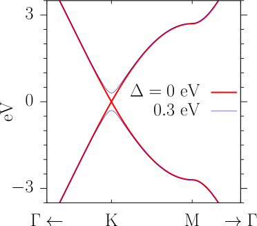
Figure 1: (Color online) Band structures of gapped graphene with different gap parameter $\Delta=0$ (red thick curves) and $0.3$ eV (blue thin curves) at $\Delta=0.3$ eV.

For later use in the discretization of the derivatives in Eq. (6), we introduce the matrix elements of $e^{-i\bm{q}\cdot\bm{r}}$ as

$$\int d\bm{r}dz\psi^{\ast}_{s_{1}\bm{k}_{1}}(\bm{r},z)e^{-i\bm{q}\cdot\bm{r}}\psi_{s_{2}\bm{k}_{2}}(\bm{r},z) = \delta(\bm{k}_{1}+\bm{q}-\bm{k}_{2})$$

$$\times U_{s_{1}\bm{k}_{1};s_{2}\bm{k}_{1}+\bm{q}}\,,$$

Here $U_{s_{1}\bm{k};s_{2}\bm{k}+\bm{q}}$ is calculated by

$$U_{s_{1}\bm{k};s_{2}\bm{k}+\bm{q}}=\sum_{\alpha_{1}\alpha_{2}}\left(c_{s_{1}\bm{k}}^{\alpha_{1}}\right)^{\ast}c_{s_{2}\bm{k}+\bm{q}}^{\alpha_{2}}W_{\alpha_{1}\bm{k};\alpha_{2}\bm{k}+\bm{q}}\,.$$

with

$$W_{\alpha_{1}\bm{k};\alpha_{2}\bm{k}+\bm{q}} = \sum_{nm}e^{-i\bm{k}\cdot\bm{R}_{nm}}\int_{\Omega}d\bm{r}dze^{-i\bm{q}\cdot\bm{r}}$$

$$\times \phi_{\alpha_{1}}^{\ast}(\bm{r}-\bm{R}_{nm}-\bm{\tau}_{\alpha_{1}},z)\phi_{\alpha_{2}}(\bm{r}-\bm{\tau}_{\alpha_{2}},z)\,.$$

For small $\bm{q}$, we approximate $W_{\alpha_{1}\bm{k};\alpha_{2}\bm{k}+\bm{q}}\approx e^{-i\bm{q}\cdot\bm{\tau}_{\alpha_{1}}}\delta_{\alpha_{1}\alpha_{2}}$ which gives

$$U_{s_{1}\bm{k};s_{2}\bm{k}+\bm{q}}=\sum_{\alpha}\left(c_{s_{1}\bm{k}}^{\alpha}\right)^{\ast}c_{s_{2}\bm{k}+\bm{q}}^{\alpha}e^{-i\bm{q}\cdot\bm{\tau}_{\alpha}}\,.$$ (2)

The Berry connections can be found from $U_{s_{1}\bm{k};s_{2}\bm{k}+\bm{q}}$ by

$$\bm{\xi}_{s_{1}s_{2}\bm{k}}=i\left.\left(\bm{\nabla}_{\bm{q}}U_{s_{1}\bm{k};s_{2}\bm{k}+\bm{q}}\right)\right|_{\bm{q}=0}\,,$$ (3)

and then the velocity matrix elements are given as $\bm{v}_{ss\bm{k}}=\hbar^{-1}\bm{\nabla}_{\bm{k}}\varepsilon_{s\bm{k}}$ and $\bm{v}_{s\bar{s}\bm{k}}=i\hbar^{-1}(\varepsilon_{s\bm{k}}-\varepsilon_{\bar{s}\bm{k}})\xi_{s\bar{s}\bm{k}}$, with $\bar{s}=+(-)$ when $s=-(+)$. After some algebra, we find

$$\bm{v}_{+-\bm{k}} = \left(c_{+\bm{k}}^{A}\right)^{\ast}c_{-\bm{k}}^{B}\bm{g}_{\bm{k}}+\left(c_{+\bm{k}}^{B}\right)^{\ast}c_{-\bm{k}}^{A}\bm{g}_{\bm{k}}^{\ast}$$ (4)

$$= \frac{1}{f_{\bm{k}}}\left\{i\text{Im}[f_{\bm{k}}\bm{g}_{\bm{k}}]+{\cal N}_{\bm{k}}\text{Re}[f_{\bm{k}}\bm{g}_{\bm{k}}]\right\}\,,$$

with $\bm{g}_{\bm{k}}=\hbar^{-1}\gamma_{0}\left[\bm{\nabla}_{\bm{k}}f_{\bm{k}}+i(\bm{\tau}_{B}-\bm{\tau}_{A})f_{\bm{k}}\right]$. We are interested in optical transitions around the Dirac points $\bm{K}=(\bm{b}_{1}+2\bm{b}_{2})/3$ and $\bm{K}^{\prime}=(2\bm{b}_{1}+\bm{b}_{2})/3$ with the primitive reciprocal lattice vectors $\bm{b}_{1}=\frac{2\pi}{a_{0}}\left(\frac{1}{\sqrt{3}}\hat{\bm{x}}-\hat{\bm{y}}\right)$ and $\bm{b}_{2}=\frac{2\pi}{a_{0}}\left(\frac{1}{\sqrt{3}}\hat{\bm{x}}+\hat{\bm{y}}\right)$. The usual approximated quantities around the Dirac points which we used are listed in Table 1.

Table 1: Lowest order approximations for $\bm{k}$ around the Dirac points. Here we use $v_{F}=\sqrt{3}a_{0}\gamma_{0}/(2\hbar)$, $\bm{\kappa}=\kappa\hat{\bm{\kappa}}$ with $\hat{\bm{\kappa}}=\cos\theta\hat{\bm{x}}+\sin\theta\hat{\bm{y}}$, $\alpha_{\kappa}={\hbar v_{F}\kappa}/{\sqrt{\Delta^{2}+(\hbar v_{F}\kappa)^{2}}}$, and $\beta_{\kappa}={\Delta}/{\sqrt{\Delta^{2}+(\hbar v_{F}\kappa)^{2}}}$

		$\bm{k}=\bm{K}+\bm{\kappa}$		$\bm{k}=\bm{K}^{\prime}+\bm{\kappa}$
$\gamma_{0}f_{\bm{k}}$		$i\hbar v_{F}\kappa e^{-i\theta}$		$i\hbar v_{F}\kappa e^{i\theta}$
$\varepsilon_{+\bm{k}}$		$\sqrt{(\hbar v_{F}\kappa)^{2}+\Delta^{2}}$,		$\sqrt{(\hbar v_{F}\kappa)^{2}+\Delta^{2}}$
$\bm{v}_{++\bm{k}}$		$\alpha_{\kappa}v_{F}\hat{\bm{\kappa}}$		$\alpha_{\kappa}v_{F}\hat{\bm{\kappa}}$
$\bm{g}_{\bm{k}}$		$v_{F}(i\hat{\bm{x}}+\hat{\bm{y}})$		$v_{F}(i\hat{\bm{x}}-\hat{\bm{y}})$
$v^{x}_{+-\bm{k}}$		$v_{F}e^{-i\theta}\left(i\beta_{\kappa}\cos\theta-\sin\theta\right)$		$v_{F}e^{i\theta}\left(i\beta_{\kappa}\cos\theta+\sin\theta\right)$
$v^{y}_{+-\bm{k}}$		$v_{F}e^{-i\theta}\left(i\beta_{\kappa}\sin\theta+\cos\theta\right)$		$v_{F}e^{i\theta}\left(i\beta_{\kappa}\sin\theta-\cos\theta\right)$

With the application of an external homogeneous electric field $\bm{E}(t)$, within the independent particle approximation the time evolution of the system can be described by SBE Cheng et al. (2015)

$$i\hbar\frac{\partial\rho_{\bm{k}}(t)}{\partial t} = [\mathcal{E}_{\bm{k}}-e\bm{E}(t)\cdot\bm{\xi}_{\bm{k}},\rho_{\bm{k}}(t)]-ie\bm{E}(t)\cdot\bm{\nabla}_{\bm{k}}\rho_{\bm{k}}(t)$$ (5)

$$+ i\hbar\left.\frac{\partial\rho_{\bm{k}}(t)}{\partial t}\right|_{\text{scat}}\,.$$

Here $\rho_{\bm{k}}$ is a single particle density matrix, for which the diagonal term $\rho_{ss\bm{k}}$ gives the occupation at state $\psi_{s\bm{k}}$ and the off-diagonal term $\rho_{+-\bm{k}}$ identifies the interband polarization between two bands; ${\cal E}_{\bm{k}}$ is the energy matrix with elements ${\cal E}_{s_{1}s_{2}\bm{k}}=\delta_{s_{1}s_{2}}\varepsilon_{s_{1}\bm{k}}$; and $e=-|e|$ is the electron charge. Although $\bm{\xi}_{\bm{k}}$ alone is a gauge dependent quantity, depending on the phases chosen for the Bloch functions, the combination with the derivative term $\bm{\nabla}_{\bm{k}}$ is gauge independent and can be written as

$$[-e\bm{E}(t)\cdot\bm{\xi}_{\bm{k}},\rho_{\bm{k}}]-ie\bm{E}(t)\cdot\bm{\nabla}_{\bm{k}}\rho_{\bm{k}}$$ (6)

$$= -ie\bm{E}(t)\cdot\left.\bm{\nabla}_{\bm{q}}\left(U_{\bm{k};\bm{k}+\bm{q}}\rho_{\bm{k}+\bm{q}}U_{\bm{k}+\bm{q};\bm{k}}\right)\right|_{\bm{q}=0}\,,$$

The term $\left.\frac{\partial\rho_{\bm{k}}(t)}{\partial t}\right|_{\text{scat}}$ describes the relaxation processes. In a phenomenological way we model the intraband (interband) relaxation process by a parameter $\Gamma_{i}$ ($\Gamma_{e}$), and then

$$\hbar\left.\frac{\partial\rho_{ss\bm{k}}(t)}{\partial t}\right|_{\text{scat}} = -\Gamma_{i}[\rho_{ss\bm{k}}(t)-\rho^{0}_{ss\bm{k}}]\,,$$

$$\hbar\left.\frac{\partial\rho_{s\bar{s}\bm{k}}(t)}{\partial t}\right|_{\text{scat}} = -\Gamma_{e}\rho_{s\bar{s}\bm{k}}(t)\,,$$ (7)

where the density matrix at equilibrium state is given by $\rho_{s_{1}s_{2}\bm{k}}^{0}=[1+e^{(\varepsilon_{s_{1}\bm{k}}-\mu)/(k_{B}T)}]^{-1}\delta_{s_{1}s_{2}}$ at temperature $T$ and chemical potential $\mu$. The current density is calculated as

$$\bm{J}(t)=e\sum_{s_{1}s_{2}}\int\frac{d\bm{k}}{(2\pi)^{2}}\bm{v}_{s_{2}s_{1}\bm{k}}\rho_{s_{1}s_{2}\bm{k}}(t)\,.$$ (8)

To focus on the nonlinear response, we separate the linear and nonlinear contributions to the perturbed density matrix by writing $\rho_{\bm{k}}(t)=\rho_{\bm{k}}^{0}+\rho_{\bm{k}}^{(1)}(t)+\rho_{\bm{k}}^{(nl)}(t)$ where $\rho_{\bm{k}}^{(1)}(t)$ is the perturbative linear contribution of the electric field and determined by

$$i\hbar\frac{\partial\rho^{(1)}_{\bm{k}}(t)}{\partial t} = [\mathcal{E}_{\bm{k}},\rho^{(1)}_{\bm{k}}(t)]-e\bm{E}(t)\cdot\{[\bm{\xi}_{\bm{k}},\rho^{0}_{\bm{k}}]+i\bm{\nabla}_{\bm{k}}\rho^{0}_{\bm{k}}\}$$ (9)

$$-i\begin{pmatrix}\Gamma_{i}\rho_{++\bm{k}}^{(1)}(t)&\Gamma_{e}\rho_{+-\bm{k}}^{(1)}(t)\\ \Gamma_{e}\rho_{-+\bm{k}}^{(1)}(t)&\Gamma_{i}\rho_{--\bm{k}}^{(1)}(t)\end{pmatrix}\,,$$

while $\rho_{\bm{k}}^{(nl)}(t)$ includes all higher order contributions and satisfies the equation

$$i\hbar\frac{\partial\rho^{(nl)}_{\bm{k}}(t)}{\partial t} = [\mathcal{E}_{\bm{k}},\rho^{(nl)}_{\bm{k}}(t)]-e\bm{E}(t)\cdot\Big{\{}[\bm{\xi}_{\bm{k}},\rho^{(1)}_{\bm{k}}(t)+\rho^{(nl)}_{\bm{k}}(t)]$$ (10)

$$+i\bm{\nabla}_{\bm{k}}[\rho^{(1)}_{\bm{k}}(t)+\rho^{(nl)}_{\bm{k}}(t)]\Big{\}}$$

$$-i\begin{pmatrix}\Gamma_{i}\rho_{++\bm{k}}^{(nl)}(t)&\Gamma_{e}\rho_{+-\bm{k}}^{(nl)}(t)\\ \Gamma_{e}\rho_{-+\bm{k}}^{(nl)}(t)&\Gamma_{i}\rho_{--\bm{k}}^{(nl)}(t)\end{pmatrix}\,,$$

The solution of Eqs. (9) and (10) completely determines the evolution of the single-particle density matrix, and the current can be written as $J^{d}(t)=J^{(1);d}(t)+J^{(nl);d}(t)$ where $J^{(1);d}(t)$ and $J^{(nl);d}(t)$ are induced by $\rho^{(1)}_{\bm{k}}(t)$ and $\rho^{(nl)}_{\bm{k}}(t)$ respectively, and describe the linear and nonlinear response.

III Numerical scheme and fitting procedure

We consider the response of the current to an applied electric field pulse with a Gaussian envelope function,

$$\bm{E}(t)=\hat{\bm{x}}E_{0}e^{-t^{2}/\Delta_{c}^{2}}e^{-i\omega_{c}t}+c.c.\,,$$ (11)

with a duration $\Delta_{c}$ and a center frequency $\omega_{c}$. In the frequency domain, this corresponds to a function with Gaussian peaks at $\pm\omega_{c}$

$$\bm{E}(\omega) = \int dte^{i\omega t}\bm{E}(t)$$

$$= \sqrt{\pi}\Delta_{c}E_{0}\left[e^{-(\omega-\omega_{c})^{2}\Delta_{c}^{2}/4}+e^{-(\omega+\omega_{c})^{2}\Delta_{c}^{2}/4}\right]\hat{\bm{x}}\,,$$

each with a spectral width $2/\Delta_{c}$.

In contrast to the numerical study by Zhang et al. Zhang and Voss (2011), where the $\bm{p}\cdot\bm{A}$ interaction is used and there is no coupling between different $\bm{k}$ points, our SBE, which is based on the $\bm{r}\cdot\bm{E}$ interaction, involve derivatives of the single-particle density matrix with respect to $\bm{k}$. In the numerical calculations, we divide the Brillouin zone (BZ) into an $M\times M$ homogeneous grid, and discretize the derivative in Eq. (6) as Marzari and Vanderbilt (1997)

$$\left.\bm{\nabla}_{\bm{q}}F(\bm{q})\right|_{\bm{q}=0}\approx\frac{a_{0}^{2}M^{2}}{16\pi^{2}}\sum_{i}\frac{\bm{q}_{i}}{M}F\left(\frac{\bm{q}_{i}}{M}\right)\,,$$ (12)

where $\bm{q}_{i}$ are chosen as six symmetric points of the honeycomb lattice

$$\{\bm{b}_{1},\bm{b}_{2},-\bm{b}_{1},-\bm{b}_{2},\bm{b}_{1}+\bm{b}_{2},-(\bm{b}_{1}+\bm{b}_{2})\}\,,$$

Throughout this work, we are interested in the optical response at different frequencies and its dependence on the electric field amplitude $E_{0}$, the chemical potential $\mu$ and the gap parameter $\Delta$. Other parameters used in the simulation are fixed as $T=300$ K, $\Delta_{c}=100$ fs, $\hbar\omega_{c}=0.6$ eV, and $\Gamma_{i}=\Gamma_{e}=33$ meV. The discrete $\bm{k}$ points are taken from a grid with $M=1500$, and included in the calculation if $\varepsilon_{+\bm{k}}<3.5$ eV; tests involving the inclusion of more $\bm{k}$ points confirm that such a restriction leads to converged numerical simulations. The time evolution of Eqs. (9) and (10) is solved by a fourth order Runge-Kutta method with a time step $\Delta t=0.05$ fs. The current in Eq. (8) is numerically calculated by summing all band indices and all the effective $\bm{k}$ points on the grid with an equal weight. After discretization, Eqs. (9) and (10) become linear differential equations for which the accuracy of the numerical solution is only limited by the time step. We point out that the density matrix $\rho_{\bm{k}}(t)$ acquires a phase dependence on $\bm{k}$ that changes with time. At long enough times $\rho_{\bm{k}}(t)$ can be strongly dependent on $\bm{k}$, and then an accurate calculation of the current from Eq. (8) requires a very dense grid, without which the nonlinear current is buried in numerical noise. Similarly, a dense grid is also required if the relaxation parameters $\Gamma_{i/e}$ are very small. However, when making calculations for the pulses and relaxation parameters we adopt here, we find that the nonlinear current can be determined reliably by the use of the moderate grid identified above.

Figure 2: (Color online) Linear optical current (a) $J^{(1);x}(t)$ (b) $J^{(1);x}(\omega)$. The parameters used in the calculation are $E_{0}=10^{6}$ V/m, $\Delta=0.10$ eV, and $\mu=0$. In (b), squares are numerical results, while the curves are fitted to $J^{(1);x}(\omega)=\sigma_{l}(\omega_{c})E^{x}(\omega)$.

We begin by illustrating the fitting procedure used in this work to extract the coefficients characterizing the optical response, and consider a weak incident optical pulse with $E_{0}=10^{6}$ V/m, $\Delta=0.10$ eV, and $\mu=0$. The linear response can be determined by solving Eq. (9) numerically, and using the result to construct $\bm{J}^{(1)}(t)$.  The result is shown in Fig. 2(a) for an incident field in the $\hat{\bm{x}}$ direction, and the Fourier transform,

$$J^{(1);x}(\omega)=\int e^{i\omega t}J^{(1);x}(t)dt$$

is numerically determined and shown in Fig. 2(b). Very generally the linear response is of the form

$$J^{(1);x}(\omega)=\sigma^{(1);xx}(\omega)E^{x}(\omega)\,,$$

and $\sigma^{(1);xx}(\omega)$ could be extracted directly for $\omega$ around $\omega_{c}$. Putting $\sigma_{l}(\omega_{c})\equiv\sigma^{(1);xx}(\omega_{c})$, the result is $\sigma_{l}(\omega_{c})=(1.11-0.05i)\sigma_{0}$, with the universal conductivity $\sigma_{0}=e^{2}/(4\hbar)$.

Figure 3: (Color online) Nonlinear optical current (a) $J^{(nl);x}(t)$, and $J^{(nl);x}(\omega)$ for $\omega$ around (b) $\omega_{c}$, (c) $2\omega_{c}$, (d) $3\omega_{c}$. The parameters used in the calculation are $E_{0}=10^{6}$ V/m, $\Delta=0.10$ eV, and $\mu=0$. In figures (b)-(d), squares are numerical results, while the curves are fitted to Eq. (15), and the fitting parameters are given in the text.

The situation is different for the nonlinear response. It can be determined by solving Eq. (10) numerically, and using the results to construct $\bm{J}^{(nl)}(t)$. The result is shown in Fig. 3(a); note that it is much smaller than the linear response, and the peak amplitude is shifted to a time slightly later than the peak of the linear response. The Fourier transform,

$$J^{(nl);x}(\omega)=\int e^{i\omega t}J^{(nl);x}(t)dt,$$

can then be numerically determined. Here we find a significant response for $\omega$ close to $\omega_{c}$ [corresponding generally to the Kerr effect and two-photon absorption, and shown in Fig. 3(b)], for $\omega$ close to $2\omega_{c}$ [corresponding to SHG, and shown in Fig. 3(c)], and for $\omega$ close to $3\omega_{c}$ [corresponding to THG, and shown in Fig. 3(d)], and of course for $\omega$ close to the associated negative frequencies. While Figs. 3(c) and 3(d) are essentially Gaussian in form, as was Fig. 2(b), Fig. 3(b) certainly is not. So the question arises as to how to characterize the nonlinear response and identify the relevant response coefficients.

In the perturbative regime, we can very generally expect a nonlinear response of the form

$$J^{(nl);x}(\omega) = \int\frac{d\omega_{1}}{2\pi}\sigma^{(2);xxx}(\omega_{1},\omega-\omega_{1})E^{x}(\omega_{1})E^{x}(\omega-\omega_{1})$$ (13)

$$+ \int\frac{d\omega_{1}d\omega_{2}}{(2\pi)^{2}}\sigma^{(3);xxxx}(\omega_{1},\omega_{2},\omega-\omega_{1}-\omega_{2})$$

$$\times E^{x}(\omega_{1})E^{x}(\omega_{2})E^{x}(\omega-\omega_{1}-\omega_{2})\,.$$

For $\omega_{i,j,k}=\pm\omega_{c}$ and small $\delta_{i,j,k}$, an approximate analytic perturbation calculation Cheng et al. (2015) leads to

$$\sigma^{(2);xxx}(\omega_{i}+\delta_{1} ,\omega_{j}+\delta_{2})\approx s_{1}^{(2)}+\frac{1\text{eV}}{\hbar(\delta_{1}+\delta_{2})+i\gamma}s_{2}^{(2)}\,,$$

$$\sigma^{(3);xxxx}(\omega_{i}+\delta_{1} ,\omega_{j}+\delta_{2},\omega_{k}+\delta_{3})\approx s_{1}^{(3)}$$ (14)

$$+\frac{1\text{eV}}{\hbar(\delta_{1}+\delta_{2}+\delta_{3})+i\gamma}s_{2}^{(3)}\,,$$

where $s_{l}^{(2)}$, $s_{l}^{(3)}$, and $\gamma$ are determined in the calculation, and take on different values for different choices of the $\omega_{i,j,k}$. Motivated by this, we fit the results of Fig. 3 by assuming the conductivity as the form of Eq. (14) with taking $s_{l}^{(2)}$, $s_{l}^{(3)}$, and $\gamma$ as free fitting parameters. This leads to a fit of the nonlinear current spectrum around $\Omega=\omega_{c},$ $2\omega_{c}$, and $3\omega_{c}$ of the form

$$J^{(n);x}(\Omega+\delta) = C_{\Omega}\left[s_{1}^{(n)}+\frac{1\text{eV}}{\hbar\delta+i\gamma}s_{2}^{(n)}\right]$$ (15)

$$\times e^{-(\delta\Delta_{c})^{2}/(4n)}\frac{\sqrt{\pi}\Delta_{c}}{\sqrt{n}}E_{0}^{n}\,.$$

Here $n=2$ is used for $\Omega=2\omega_{c}$, and $n=3$ for $\Omega=\omega_{c}$ or $3\omega_{c}$, with $C_{\Omega}$ describing the permutation factor relevant for the nonlinear process; $C_{\omega_{c}}=3$, and $C_{2\omega_{c}}=C_{3\omega_{c}}=1$. The result of this fitting is shown by the solid curves in Fig. 3(b)-3(d), and we can see that indeed a very good fit is provided. Once the fit of Eq. (15) is accepted, we can return to Eq. (14) and identify the nonlinear response coefficients $\sigma^{(2);xxx}(\omega_{c},\omega_{c})$ (associated with SHG for a fundamental at $\omega_{c}$), $\sigma^{(3);xxxx}(\omega_{c},\omega_{c},\omega_{c})$ (associated with THG for a fundamental at $\omega_{c}$), and $\sigma^{(3);xxxx}(-\omega_{c},\omega_{c},\omega_{c})$ (associated with the Kerr effect and two-photon absorption for a fundamental at $\omega_{c}$). For the results shown in Fig. 3, for example, we find $\sigma_{0}^{-1}\sigma^{(2);xxx}(\omega_{c},\omega_{c})=(-37.2+16.5i)$ pm/V, with $s_{2}^{(2)}\sim 0$; $\sigma_{0}^{-1}\sigma^{(3);xxxx}(\omega_{c},\omega_{c},\omega_{c})=(0.91+0.04i)\times 10^{-19}$ m²/V² with $s_{2}^{(3)}\sim 0$; and $\sigma_{0}^{-1}\sigma^{(3);xxxx}(-\omega_{c},\omega_{c},\omega_{c})=(-4.1+0.2i)\times$ $10^{-16}$ m²/V² with $\sigma_{0}^{-1}s_{1}^{(3)}=(1463.5+239.7i)\times 10^{-19}$m²V², $\sigma_{0}^{-1}s_{2}^{(3)}=(0.9-202.5i)\times 10^{-19}$ m²/V², and $\gamma=36.3$ meV.

For weak incident fields, we can use this strategy to extract coefficients $\sigma^{(2);xxx}(\omega_{c},\omega_{c})$, $\sigma^{(3);xxxx}(\omega_{c},\omega_{c},\omega_{c})$ and $\sigma^{(3);xxxx}(-\omega_{c},\omega_{c},\omega_{c})$ from our numerical calculations, confirm that they are independent of the amplitude $E_{0}$ of the incident field – as they should be in the perturbative regime – and compare them with the results of the approximate but analytic expressions for these response coefficients. For strong incident fields a strict perturbative response of the form in Eq. (14) is not expected to hold. Still, the nonlinear response can be expected to be characterized by SHG, THG, and terms that behave phenomenologically as Kerr and two-photon absorption effects. Thus from our numerical calculations we can extract an effective $\sigma^{(2);xxx}(\omega_{c},\omega_{c})$ [which we denote as $\sigma_{\text{SHG}}(\omega_{c})$], an effective $\sigma^{(3);xxxx}(\omega_{c},\omega_{c},\omega_{c})$ [which we denote as $\sigma_{\text{THG}}(\omega_{c})$] and an effective $\sigma^{(3);xxxx}(-\omega_{c},\omega_{c},\omega_{c})$ [which we denote as $\sigma_{nl}(\omega_{c})$]. Unlike the coefficients that govern the perturbative regime, we can expect the effective coefficients $\sigma_{\text{SHG}}(\omega_{c})$, $\sigma_{\text{THG}}(\omega_{c})$, and $\sigma_{nl}(\omega_{c})$ to depend on the amplitude of the electric field strength, containing renormalizations of the perturbative response coefficients in the presence of strong fields.

Using the fitting scheme described above, we study two examples of the dependence of the effective conductivities on the chemical potential $\mu$, the gap parameter $\Delta$, and the electric field amplitude $E_{0}$. In the first we consider the dependence on $\mu$ and $E_{0}$ with $\Delta=0$, which we refer to as doped graphene (DG). In the second we consider the dependence on $\Delta$ and $E_{0}$ with $\mu=0$, which we refer to as undoped gapped graphene (GG).

IV Results

IV.1 Comparing numerical calculations to analytic perturbation results

Figure 4: (Color online) The linear effective conductivities for DG (squares) and GG (dots) for $E_{0}=10^{6}$ V/m. The curves are calculated from Eq. (16) for DG and Eq. (17) for GG.

As a benchmark, we first compare the numerical effective conductivities at a weak electric field $E_{0}=10^{6}$ V/m with those available from analytic perturbation calculations. We begin with the linear response. For DG, in previous work Cheng et al. (2015) we presented the analytic expression for $\sigma^{(1);xx}(\omega)$ obtained perturbatively from the same SBE as Eq. (5), taking into account both interband and intraband relaxation coefficients $\Gamma_{e}$ and $\Gamma_{i}$ respectively, but using matrix elements and energies correct only around the Dirac points; our analytic result is

$$\sigma_{\text{DG}}^{(1)xx}(\omega;|\mu|)=\beta\int_{-\infty}^{\infty}\!\!\!F_{\mu}(x,T)[1-F_{\mu}(x,T)]\sigma_{\text{DG};0}^{(1)xx}(\omega;x)dx\,,$$ (16)

where $\beta=1/(k_{B}T)$ with $k_{B}$ Boltzmann’s constant, and $F_{\mu}(x,T)=[1+e^{\beta(x-\mu)}]^{-1}$. The conductivity at zero temperature is

$$\sigma_{\text{DG};0}^{(1);xx}(\omega;\mu)=\frac{i\sigma_{0}}{\pi}\left\{-{\cal G}_{|\mu|}(\hbar\omega+i\Gamma_{e})+\frac{4|\mu|}{\hbar\omega+i\Gamma_{i}}\right\}\,.$$

Here the function ${\cal G}_{|\mu|}(\theta)$ is given for $\theta=\theta_{r}+i\theta_{i}$ as

$${\cal G}_{|\mu|}(\theta) =\ln\left|\frac{2|\mu|+\theta}{2|\mu|-\theta}\right|+i\left(\pi+\arctan\frac{\theta_{r}-2|\mu|}{\theta_{i}}\right.$$

$$\left.-\arctan\frac{\theta_{r}+2|\mu|}{\theta_{i}}\right)\,.$$

For GG, because the chemical potential is taken as $0$ and the gap is nonzero, the net contribution to the linear conductivity from the intraband transitions (Drude term) vanishes at zero temperature; even at room temperature that contribution is negligible, so for GG we can restrict the expression for the linear conductivity to its interband component,

$$\sigma_{\text{GG};\text{inter}}^{(1);xx}(\omega) = e^{2}\sum_{s\bm{k}}\frac{v_{\bar{s}s\bm{k}}^{x}\xi^{x}_{s\bar{s}\bm{k}}(n_{s\bm{k}}-n_{\bar{s}\bm{k}})}{\hbar\omega-(\varepsilon_{{s}\bm{k}}-\varepsilon_{\bar{s}\bm{k}})+i\Gamma_{e}}$$ (17)

$$= \frac{i\sigma_{0}}{\pi}\left\{-{\cal G}_{\Delta}(\hbar\omega+i\Gamma_{e})+\frac{4\Delta}{\hbar\omega+i\Gamma_{e}}\right\}$$

$$-\frac{i\sigma_{0}}{\pi}\frac{(2\Delta)^{2}}{(\hbar\omega+i\Gamma_{e})^{2}}{\cal G}_{\Delta}(\hbar\omega+i\Gamma_{e})\,.$$

In Fig. 4 we plot the results extracted from our numerical simulations of Eq. (9), together with the analytic results in Eq. (16) and (17) as a function of $\mu$ (for DG) and $\Delta$ (for GG). The agreement is very good.

Figure 5: (Color online) Nonlinear response for DG and GG: the nonlinear conductivity $\sigma_{0}^{-1}\sigma_{nl}(\omega_{c})$ and $\sigma_{0}^{-1}\sigma_{\text{THG}}(\omega_{c})$ at (a), (b) $E_{0}=10^{6}$ V/m and (e), (f) $2\times 10^{7}$ V/m; $J^{(nl)}(\omega)$ of GG with $\Delta=0.20$, $0.25$, $0.30$, and $0.35$ eV for $\omega$ around (c) $\omega_{c}$ and (d) $3\omega_{c}$. The $y$-axis for the real (imaginary) parts of $J^{(nl)}(\omega)$ is at the left (right) hand side of (c) and (d). Solid curves are calculated from analytic perturbation results Cheng et al. (2015) for DG; dashed curves are drawn to guide the eye.

Turning next to the third order response, for the analytic expressions of $\sigma^{(3);xxxx}(-\omega_{c},\omega_{c},\omega_{c})$ and $\sigma^{(3);xxxx}(\omega_{c},\omega_{c},\omega_{c})$ relevant for DG we use our previous results Cheng et al. (2015), including both interband and intraband relaxation, and with matrix elements and energies taken to be those that characterize the regions about the Dirac points. For GG with a nonzero gap parameter, perturbative results for THG were obtained by Jafari Jafari (2012), but instead of using the SBE in Eq. (5) a Kubo formula based on the ${\bm{p}}\cdot{\bm{A}}$ interaction was used, without the inclusion of any relaxation. Thus while we present our numerical results for $\sigma_{nl}(\omega_{c})$ and $\sigma_{\text{THG}}(\omega_{c})$ for both DG and GG, we only compare with the relevant analytic results from perturbation theory obtained for DG. This is shown in Figs. 5(a) and 5(b) for $\sigma_{nl}(\omega_{c})$ and $\sigma_{\text{THG}}(\omega_{c})$ respectively at $E_{0}=10^{6}$ V/m. The numerical and analytic results for DG match very well for chemical potentials over the range shown. There is a noticeable difference between the numerical and analytically results for $\text{Re}[\sigma_{nl}(\omega_{c})]$, although it is less than $10\%$, for $\mu<0.3$ eV. We can attribute this to the singular behavior that $\text{Re}[\sigma_{nl}(\omega_{c})]$ exhibits in the perturbative calculation Cheng et al. (2015) for $|\mu|<\hbar\omega_{c}/2$, here $|\mu|<0.3$ eV. Associated with this, the nonlinear current in the numerical calculation shows a very strong dependence on the pulse duration and shape, and the strategy identified above for extracting $\sigma_{nl}(\omega_{c})$ from the pulse calculation is not completely successful.

The very good agreement at $E_{0}=10^{6}$ V/m between the effective conductivities of DG extracted from the numerical calculations, and the conductivities predicted by the analytic perturbation theory, suggests that Eqs. (14) and (15) provide a reasonable fitting procedure, and as well that for weak fields the perturbative results presented earlier Cheng et al. (2015) are reliable. It also indicates that the usual Dirac point approximations adopted in the perturbative calculation, involving the linear dispersion relation and the form of the matrix elements, do not introduce any significant errors in calculating the linear and nonlinear optical response of DG at incident photon energies around $\hbar\omega=0.6$ eV.

We also see from Figs. 5(a) and 5(b) that there is a similarity in the dependence of the DG results on $\mu$ with the dependence of the GG results on $\Delta$. Before turning to the response of both system at larger field strengths, we address such similarities in the following section.

IV.2 Comparing DG and GG

In investigations of the optical conductivities of doped graphene, $2|\mu|$ is often treated as an effective gap Cheng et al. (2014a, 2015). Since GG has a real gap of $2\Delta$, it is interesting to compare the dependence of the optical conductivities on the effective gap $2|\mu|$ induced by the chemical potential in DG with the real gap $2\Delta$ arising in GG. In linear response, some insight can be gleaned by comparing the analytic formulas in Eq. (16) and (17) for DG and GG. In Eq. (17) the interband velocity matrix elements $\bm{v}_{+-{\bm{k}}}$ depend on $\beta_{\bm{\kappa}}$, as shown in Table 1, and through that dependence they depend on $\Delta$. If $\beta_{\bm{\kappa}}$ were not present, only the first term in the bracket of Eq. (17) would survive, corresponding to the interband contribution to the conductivity of DG Cheng et al. (2015) with $|\mu|$ replaced by $\Delta$. The presence of $\beta_{\bm{\kappa}}$ leads to the appearance of the other two contributions. Interestingly, one has the same form as the Drude term in DG (with $|\mu|$ replaced by $\Delta$), while the other is new.

The consequences of the second new term in GG are apparent in the results shown in Fig. 4; the main differences between the DG and GG results is that around $\hbar\omega_{c}\approx 2\Delta$ the latter show a deeper valley in the imaginary part of the conductivity, and a larger peak in the real part of the conductivity. The real part of the conductivity is associated with absorption, and through Fermi’s Golden Rule it is determined by both the joint density of states and the velocity matrix elements. Now for GG the joint density of states for energies around the Dirac points is given by

$${\cal D}(\epsilon)=2\sum_{\bm{k}}\delta(\epsilon-(\varepsilon_{+\bm{k}}+\varepsilon_{-\bm{k}}))=\frac{\epsilon}{2\pi(\hbar v_{F})^{2}}\theta(\epsilon-2\Delta)\,,$$

where the factor $2$ comes from the spin degeneracy. Comparing with DG, the joint density of states is the same for $\epsilon>2|\mu|$ in DG as it is for $\epsilon>2\Delta$ in GG, and so at such energies the differences in the linear conductivity should be associated with the velocity matrix elements; and indeed, they can be linked to the last term in Eq. (17).

Turning to the nonlinear response, we first compare the DG and GG results for $\sigma_{nl}(\omega_{c})$, shown in Fig. 5(a). The result for GG shows fine structure as $\Delta$ is close to $\hbar\omega_{c}/2$. For $\Delta<\hbar\omega_{c}/2$ both one- and two-photon absorption are present, and $\text{Re}[\sigma_{nl}(\omega_{c})]$ is negative and increases in magnitude with increasing $\Delta$. In a manner similar to what is shown by the results of perturbative calculations Cheng et al. (2014a, 2015) at $|\mu|<\hbar\omega_{c}/2$ for DG, we expect that at $\Delta<\hbar\omega_{c}/2$ for GG the two-photon absorption is associated with saturation as described at the level of the third-order nonlinearity; it would diverge when relaxation effects are not included. For $\Delta>\hbar\omega_{c}/2$, where only two-photon absorption exists, the negative value of $\text{Re}[\sigma_{nl}(\omega_{c})]$ is induced by the inclusion of the relaxation Cheng et al. (2015). Maximum absolute values of the imaginary and real parts of $\sigma_{nl}(\omega_{c})$ occur for GG around $\Delta=\hbar\omega_{c}/2$, and the differences between the results for GG and DG can again be attributed to the velocity matrix elements.

We turn to the results for $\sigma_{\text{THG}}(\omega_{c})$ shown in Fig. 5(b). The expected similarity of the results for GG and DG, respectively as a function of $\Delta$ and $|\mu|$, fails mainly for $\Delta,\mu>0.25$ eV. Here $\text{Re}\left[\sigma_{\text{THG}}(\omega_{c})\right]$ for GG increases faster than that of DG, as functions of $\Delta$ and $|\mu|$ respectively, while the dependences of $\text{Im}[\sigma_{\text{THG}}(\omega_{c})]$ for GG and DG are analogous, but with larger absolute values for GG. Again these differences can be traced back to the different velocity matrix elements.

Here we shortly discuss the relation between the fitted effective conductivity at $\omega_{c}$ and the amplitude of the optical current calculated from a laser pulse. As in Eq. (14), the conductivity shows a strong frequency dependence, and thus the value of the conductivity $\sigma_{nl}(\omega_{c})$ at the center frequency of a light pulse is generally not a good indication of the amplitude of the optical response $J^{(nl);x}(\omega)$ if an exciting pulse of light is actually used. The numerical results for $J^{(nl);x}(\omega)$ are shown for GG at $\omega$ close to $\omega_{c}$ in Fig. 5(c), and for $\omega$ close to $3\omega_{c}$ in Fig. 5(d), for $\Delta=0.20$, $0.25$, $0.30$, and $0.35$ eV. At $\Delta=\hbar\omega_{c}/2=0.30$ eV, both the real and imaginary parts of the nonlinear optical current [black curves in Fig. 5(c)] show a different shape than those at other $\Delta$, although they do not really exceed them in amplitude. In contrast, there is no obvious shape distortion in the spectrum shown in Fig. 5(d). As such, the values of $\sigma_{\text{THG}}(\omega_{c})$ are consistent with the magnitude of the optical current of the THG components.

The results for $\sigma_{nl}(\omega_{c})$ and $\sigma_{\text{THG}}(\omega_{c})$ extracted from the numerical results for a larger $E_{0}=2\times 10^{7}$ V/m are shown for both GG and DG in Fig. 5(e) and 5(f). Note that the dependence of the effective coefficients of DG on $\left|\mu\right|$, and those of GG on $\Delta$, are similar in nature to the dependence of those effective coefficients at $E_{0}=10^{6}$ V/m, but they take on different values. Hence we are now beyond the perturbative regime, and cannot link the effective coefficients $\sigma_{nl}(\omega_{c})$ and $\sigma_{\text{THG}}(\omega_{c})$ with the perturbative results for $\sigma^{(3);xxxx}(-\omega_{c},\omega_{c},\omega_{c})$ and $\sigma^{(3);xxxx}(\omega_{c},\omega_{c},\omega_{c})$ respectively. For $\sigma_{nl}(\omega_{c})$ there are significant differences between the values at $E_{0}=10^{6}$ V/m and at $E_{0}=2\times 10^{7}$ V/m at all values of $|\mu|$ (or $\Delta$), while for $\sigma_{\text{THG}}(\omega_{c})$ the differences are substantial only for $\Delta,|\mu|<0.3$ eV. We attribute these differences to saturation effects, which we discuss in the next section.

IV.3 Saturation effects

We now turn to the dependence of the effective coefficients $\sigma_{nl}(\omega_{c})$ and $\sigma_{\text{THG}}(\omega_{c})$ on field strength. We begin with $\sigma_{nl}(\omega_{c})$, and note that there are two different regimes that we can identify for both DG and GG:

(i) $2|\mu|<\hbar\omega_{c}$ for DG, or $2\Delta<\hbar\omega_{c}$ for GG. Here one photon absorption exists and carriers can be injected from the “$-$” band to the “$+$” band. Stronger electric fields inject more carriers. If the electrons have a finite lifetime in the states into which they are injected, their injection prevents the effectiveness of further absorption. Phenomenologically, the effect of the injected carriers on the total absorption $\alpha$ is often characterized by introducing a saturation field strength $E_{\text{sat}}$,

$$\alpha=\frac{\alpha_{0}}{1+\left({E}/{E_{\text{sat}}}\right)^{2}}$$ (18)

with $\alpha_{0}$ the linear absorption and $E$ the electric field amplitude in an assumed continuous wave excitation at frequency $\omega$. For isolated graphene, the absorption of normally incident light is proportional to $\text{Re}[\sigma_{\text{eff}}^{xx}(\omega)]$, where $\sigma_{\text{eff}}^{xx}(\omega)$ is a field dependent effective conductivity, and we would expect

$$\text{Re}[\sigma_{\text{eff}}^{xx}(\omega)]=\frac{\text{Re}[\sigma^{(1);xx}(\omega)]}{1+\left({E}/{E_{\text{sat}}}\right)^{2}}\,.$$ (19)

However, at weak fields we have Boyd (2008)

$$\sigma_{\text{eff}}^{xx}(\omega)=\sigma^{(1);xx}(\omega)+3\sigma^{(3);xxxx}(\omega,\omega,-\omega)E^{2}\,,$$ (20)

where $\sigma^{(3);xxxx}(\omega,\omega,-\omega)$ is the third order conductivity resulting from a perturbative calculation. Comparing with the weak field expansion of Eq. (19) we find

$$E_{\text{sat}}=\sqrt{-\frac{\text{Re}[\sigma^{(1);xx}(\omega)]}{3\text{Re}[\sigma^{(3);xxxx}(-\omega,\omega,\omega)]}}\,.$$ (21)

For strong electric fields, we assume that Eqs. (19) and (20) work for a field dependent conductivity $\sigma_{nl}(\omega_{c})$; further, since we extract $\sigma_{nl}(\omega_{c})$ from a numerical calculation with the incident field in Eq. (11) we can identify

$$\sigma_{\text{eff}}^{xx}(\omega_{c})=\sigma^{(1);xx}(\omega_{c})+3\sigma_{nl}(\omega_{c})E_{0}^{2}\,,$$

for $\Delta_{c}>\hbar/\Gamma_{i,e}$ where the pulsed excitation approaches continuous wave excitation, and we can replace $E$ by $E_{0}$ in Eq. (19); then we find

$$\text{Re}[\sigma_{nl}(\omega)]=-\frac{\text{Re}[\sigma^{(1);xx}(\omega)]}{3E_{\text{sat}}^{2}}\frac{1}{1+\left({E_{0}}/{E_{\text{sat}}}\right)^{2}}\,.$$ (22)

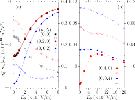
Figure 6: (Color online) Electric field dependence of the nonlinear conductivities $\sigma_{nl}(\omega_{c})$ for different $(\mu,\Delta)$. (a) $(0,0)$ (squares), $(0.2,0)$ eV (circles), and $(0,0.2)$ eV (diamonds). (b) $(0.4,0)$ (squares) and $(0,0.4)$ eV (diamonds). The real and imaginary parts are given by filled and hollow symbols, and their scales are at the left and right $y$ axis, respectively. The solid curves in (a) are fitted by functions $-\frac{\sigma_{f}}{3E_{\text{sat}}^{2}}\frac{1}{1+(E_{0}/E_{\text{sat}})^{2}}$ with two fitting parameters $\sigma_{f}$ and $E_{\text{sat}}$, while the dashed curves are drawn to guide the eye.

In Fig. 6(a) we plot the dependence of the numerically determined $\sigma_{nl}(\omega_{c})$ as a function of $E_{0}$ for three different parameter sets $(\mu,\Delta)=(0,0)$, $(0.2,0)$, and $(0,0.2)$ eV. The real part of $\sigma_{nl}(\omega_{c})$ is fitted to an expression $-{\sigma_{f}}/{[3(E_{\text{sat}}^{2}+E_{0}^{2})]}$ with two parameters $\sigma_{f}$ and $E_{\text{sat}}$. We find that the fittings (shown as solid curves) are very good for $\text{Re}[\sigma_{f}]/\sigma_{0}\approx-1$, $-1$, and $-1.53$ respectively, with the saturation fields the same in all cases as $E_{\text{sat}}\approx 3\times 10^{7}$ V/m. Comparing the fitted form with Eq. (22), and noting that the linear conductivities are given by $\sigma^{(1);xx}(\omega_{c})/\sigma_{0}=1$, $0.96-0.11i$, and $1.38-0.36i$ respectively for our parameter sets, the closeness of the fitted $\sigma_{f}$ with these linear conductivity $\sigma^{(1);xx}(\omega_{c})$ indicates that the saturation can indeed be attributed to linear absorption. Further, by using the numerical values of $\sigma_{nl}(\omega_{c})/\sigma_{0}$ at a weak field value $E_{0}=10^{6}$ V/m, which for our three parameter sets are $-3.7\times 10^{-16}$, $-3.7\times 10^{-16}$, and $-5.7\times 10^{-16}$ m²/V² respectively, Eq. (21) leads to saturation fields of $3\times 10^{7}$, $3\times 10^{7}$, and $2.8\times 10^{7}$ V/m, which are very close to the fitted values. The field dependence of $\text{Im}[\sigma_{nl}(\omega_{c})]$, which at least in the weak field limit can be related to the real part of the nonlinear response via nonlinear Kramers-Kronig relations, varies in a more complicated way.

The saturation field can also be estimated from only the linear absorption coefficients. Physically, the saturation effect occurs when the injected electron density from one-photon absorption is comparable to the density of states in the region of $\bm{k}$ space where the electrons are injected. The injected electron density is $\hbar/\Gamma_{i}\xi^{xx}(\omega_{c})E_{m}^{2}$ with the one-photon absorption coefficients Cheng et al. (2014a) $\xi^{xx}(\omega_{c})=2\text{Re}[\sigma^{(1);xx}(\omega_{c})]/(\hbar\omega_{c})$ and the critical field amplitude $E_{m}$, while the total available states are estimated as those satisfying $-\Gamma_{e}\leq\varepsilon_{+\bm{k}}-\varepsilon_{-\bm{k}}-\hbar\omega_{c}\leq\Gamma_{e}$, which has a density $\int_{\hbar\omega_{c}-\Gamma_{e}}^{\hbar\omega_{c}+\Gamma_{e}}{\cal D}(\epsilon)d\epsilon$. Then the critical field amplitude $E_{m}$ is estimated as

$$E_{m}\approx\sqrt{\frac{2\Gamma_{i}\Gamma_{e}}{\pi}\frac{\sigma_{0}}{\text{Re}[\sigma^{(1);xx}(\omega_{c})]}}\frac{\hbar\omega_{c}}{\hbar|e|v_{F}}\,.$$ (23)

This can be used to find approximate values of $E_{m}\sim 2.8\times 10^{7}$ V/m for those two parameter sets considered for DG, and $E_{m}\sim 2.4\times 10^{7}$ V/m for the parameter set considered for GG. Both values are close to the fitted saturation field.

(ii) $2|\mu|>\hbar\omega_{c}$ for DG, or $2\Delta>\hbar\omega_{c}$ for GG. Here we focus on the frequency regimes $2|\mu|>\hbar\omega_{c}>|\mu|$ or $2\Delta>\hbar\omega_{c}>\Delta$ where two photon absorption exists. Two photon absorption can inject carriers, but it is less efficient than one photon absorption. Thus saturation requires higher electric fields, and Eq. (19) does not correctly describe the physics, as shown in Fig. 6(b) for two parameter sets $(\mu,\Delta)=(0.4,0)$ and $(0,0.4)$ eV, which has different tendencies compared to the curves in Fig. 6(a). For the electric field up to $E_{0}=2\times 10^{8}$ V/m, the imaginary part of $\sigma_{nl}(\omega_{c})$ does not change much for either of these examples. The real part of $\sigma_{nl}(\omega_{c})$ of DG changes from negative values to positive values around $E_{0}\sim 4\times 10^{7}$ V/m; while that of GG remains positive and decreases. For photon energies where even two photon absorption is absent, we believe that saturation can only occur for much higher electric fields.

Figure 7: (Color online) Electric field dependence of the nonlinear conductivities $\sigma_{\text{THG}}(\omega_{c})$ for different $(\mu,\Delta)$. (a) $(0,0)$ (squares), $(0.2,0)$ eV (circles), and $(0,0.2)$ eV (diamonds). (b) $(0.4,0)$ (squares) and $(0,0.4)$ eV (diamonds). The real and imaginary parts are given by filled and hollow symbols, and their scales are at the left and right $y$ axis, respectively. The dashed curves are drawn to guide the eye.

We now turn from $\sigma_{nl}(\omega_{c})$ to $\sigma_{\text{THG}}(\omega_{c})$. We find that saturation can significantly affect THG, as shown in Figs. 7(a) and 7(b). Here again the regimes (i) and (ii) identified above are relevant. For the results shown in Fig. 7(a) we are in regime (i), where both one- and two-photon absorption are present. Here both the real and imaginary parts of $\sigma_{\text{THG}}(\omega_{c})$ depend strongly on the electric field. The imaginary part even changes its sign from positive to negative values with increasing the electric field, while the real part shows peaks around $E_{0}=5\times 10^{7}$ V/m. Compared to the values at $E_{0}=10^{6}$ V/m, these peak absolute values are about 5 times larger. In the measurement of THGSäynätjoki et al. (2013); Kumar et al. (2013); Hong et al. (2013) the procedure used to prepare the samples would indicate the chemical potentials should be very low; thus saturation may well occur and the effective THG coefficients $\sigma_{\text{THG}}(\omega_{c})$ may be above their perturbative values. For the results shown in Fig. 7(b) we are in regime (ii), where one-photon absorption is absent but two-photon absorption is still present. Here the real parts of the $\sigma_{\text{THG}}(\omega_{c})$ weakly depend on the electric field; however, their imaginary parts still strongly depend on the electric field and change the sign at about $E_{0}=10^{8}$ V/m.

Figure 8: (Color online) ${\cal S}(\epsilon)$ at $\hbar\omega_{c}=0.6$ eV, $T=300$ K, and $\Gamma_{i}=\Gamma_{e}=33$ meV. Those two vertical dashed lines are at $\epsilon=0.3$ and $0.6$ eV respectively.

To qualitatively understand how the saturation affects THG, we construct a function

$${\cal S}(\epsilon)=\sigma_{0}^{-1}\frac{d}{d\epsilon}\sigma^{(3);xxxx}(\omega_{c},\omega_{c},\omega_{c};|\epsilon|)\,,$$ (24)

Here $\sigma^{(3);xxxx}(\omega_{c},\omega_{c},\omega_{c};|\mu|)$ is the analytic perturbative third order conductivity of DGCheng et al. (2015) at zero temperature, with the chemical potential dependence explicitly shown; ${\cal S}(\epsilon)$ describes the contribution of the electron states at energy $\epsilon$ to the THG. For our calculation parameters, $\hbar\omega_{c}=0.6$ eV, $T=300$ K, and $\Gamma_{i}=\Gamma_{e}=33$ meV, the $\epsilon$ dependence of ${\cal S}(\epsilon)$ is shown in Fig. 8. For a given $\epsilon$, $\int_{\epsilon-\delta}^{\epsilon+\delta}{\cal S}(E)dE$ is the contribution to the THG of the electrons distributed in the energy range $[\epsilon-\delta,\epsilon+\delta]$. When the saturation is induced by the one-photon absorption, the electrons are injected into states with energy around $\hbar\omega_{c}/2$ from states with energy around $-\hbar\omega_{c}/2$. The contribution of the population changes to the THG is approximately $\propto\left[{\cal S}(\hbar\omega_{c}/2)-{\cal S}(-\hbar\omega_{c}/2)\right]E_{0}^{2}$, with $E_{0}^{2}$ originating from the one-photon injection carrier density. Similarly, the carriers injected by two-photon absorption contribute $\propto\left[{\cal S}(\hbar\omega_{c})-{\cal S}(-\hbar\omega_{c})\right]E_{0}^{4}$, with $E_{0}^{4}$ originating from the two-photon injection carrier density. Figure 8 shows the real parts of these two terms are positive and negative respectively. Thus they give competing contributions. For the results in Fig. 7(a), at small $E_{0}$, one-photon absorption dominates, and $\text{Re}[\sigma_{\text{THG}}(\omega_{c})]$ increases with $E_{0}$; at high $E_{0}$, two-photon absorption starts to play a role, and the appearance of a peak of $\text{Re}[\sigma_{\text{THG}}(\omega_{c})]$ is possible. The imaginary part and the results shown in Fig. 7(b) can also be understood in the same way.

IV.4 Second harmonic generation

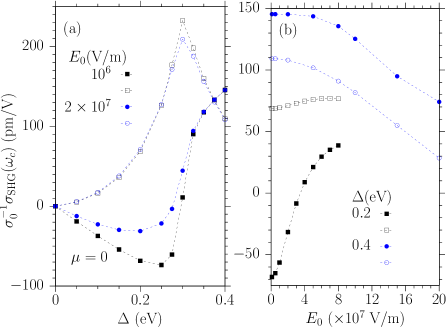
Figure 9: (Color online) (a) $\Delta$ dependence of $\sigma_{\text{SHG}}(\omega_{c})$ in GG at different electric fields $E_{0}=10^{6}$ V/m (squares) and $2\times 10^{7}$ V/m (circles), (b) electric field dependence of $\sigma_{\text{SHG}}(\omega_{c})$ at different $\Delta=0.2$ eV (squares) and $\Delta=0.4$ eV (circles). The real and imaginary parts are given by filled and hollow symbols respectively. The dashed lines are drawn to guide the eye.

Finally, we consider the dependence of SHG in GG on the band gap and electric field amplitude. In parallel with our strategy for the third order response, we introduce an effective second-order nonlinear conductivity $\sigma_{\text{SHG}}(\omega_{c})$ which is given by $\sigma^{(2);xxx}(\omega_{c},\omega_{c})$ in the weak field limit, and extracted for larger fields from the numerical calculations as sketched in section III. Our results are shown in Fig. 9(a) and 9(b). As expected, a nonzero $\Delta$, associated with the lack of centre-of-inversion symmetry, leads to a nonzero SHG response. As $\Delta$ is increased from $0$ to $0.4$ eV, the real part of $\sigma_{0}^{-1}\sigma_{\text{SHG}}(\omega_{c})$ decreases from $0$ to a negative minimum value (about $-70$ pm/V for $E_{0}=10^{6}$ V/m and $-30$ pm/V for $E_{0}=2\times 10^{7}$ V/m) around $\Delta=0.25$ eV, then changes sign around $\Delta=0.3$ eV and reaches a value about $140$ pm/V at $\Delta=0.4$ eV; they show a strong electric field dependence around the minimum values. The imaginary part of $\sigma_{0}^{-1}\sigma_{\text{SHG}}(\omega_{c})$ has positive values with a peak $\sim 200$ pm/V around $\Delta=0.3$ eV for both electric field amplitudes considered. Physically, $\sigma_{\text{SHG}}(\omega_{c})$ vanishes as $\Delta=0$, where the centre-of-inversion symmetry is present, and as $\Delta\to\infty$; for large $\Delta$ it vanishes as Boyd (2008) $\propto\Delta^{-4}$. Therefore the existence of a maximum of the magnitude of $\sigma_{\text{SHG}}(\omega_{c})$ as $\Delta$ is increased is not surprising.

To focus on the electric field dependence of $\sigma_{\text{SHG}}(\omega_{c})$, we plot that dependence in Fig. 9(b) for two gap parameters, $\Delta=0.2$ eV and $\Delta=0.4$ eV. The real part of $\sigma_{\text{SHG}}(\omega_{c})$ at $\Delta=0.2$ eV shows a strong dependence. It changes its sign from negative to positive as the electric field increases from $0$ to $8\times 10^{7}$ V/m. The reason is similar to the electric field dependence of the third order conductivities, and is induced by the saturation effects. However, the imaginary part changes little over the same range of the electric field. For $\Delta=0.4$ eV, where the saturation effects can be ignored, both the real and imaginary parts show minor changes up to a electric field $20\times 10^{7}$ V/m.

Similar to the estimation for the effective third order susceptibilitiesCheng et al. (2014a, 2015), we calculate the magnitude of the susceptibility of SHG in GG, by employing the conversion of $\chi^{(2)}(\omega_{c})\approx\sigma_{\text{SHG}}(\omega_{c})/(-2i\omega_{c}\epsilon_{0}d_{\text{gr}})$ with the effective thickness of graphene $d_{\text{gr}}=3.3$ Å. For maximum values of $|\sigma_{0}^{-1}\sigma_{\text{SHG}}|\sim 200$ pm/V around $\Delta=0.3$ eV, we get $\chi^{(2)}\sim 2300$ pm/V. This value is about 30 times higher than the widely used AgGaSe₂ crystal value $68$ pm/V at the same photon energyWu et al. (2012), or a few times larger than that of monolayer BN, which has a much larger band gap Guo and Lin (2005); Grüning and Attaccalite (2014).

V Conclusion and discussion

In this work, we numerically solved the semiconductor Bloch equations, including phenomenological relaxation times, for the excitation of both doped and gapped graphene excited by a pump pulse, and extracted the effective optical nonlinear conductivities for second harmonic generation, the Kerr effects, and third harmonic generation for a given fundamental photon energy $\hbar\omega_{c}=0.6$ eV. We focused on the dependence of these nonlinear coefficients on the chemical potential $\mu$ for doped graphene, the gap parameter $\Delta$ for gapped graphene, and the electric field amplitude for both. We obtained the following results.

(1) For doped graphene: At weak electric fields, all extracted conductivities (both linear and nonlinear) are in good agreement with the perturbation results, which is a strong evidence of the correctness of both the numerical and perturbation calculations. The numerical results also confirm that both the linear dispersion approximation and the consideration of only optical transitions around the Dirac points are physically appropriate in the perturbation calculation with using the standard $\bm{r}\cdot\bm{E}$ interaction. With an increase in the electric field amplitude, the effective Kerr coefficient shows a dependence on the field strength, which can be attributed to saturation effects. For $\hbar\omega_{c}>2|\mu|$ where one-photon absorption exists, the saturation effects can be characterized by a saturation field, which for our relaxation parameters takes a value of about $3\times 10^{7}$ V/m. The amplitude of the effective third harmonic generation coefficient can increase up to 5 times as the electric field changes from $10^{6}$ V/m to $8\times 10^{7}$ V/m. However, compared to the two orders of magnitude difference between the values from the perturbation calculation and experiments Cheng et al. (2014a, 2015), this small increment indicates that other effects, such as the consequences of including more realistic scattering and many-body phenomena, may be important.

(2) For gapped graphene: The third-order optical conductivity for both Kerr effect and third harmonic generation in gapped graphene shows obvious peaks or valleys in its $\Delta$ dependence, which is different from the $|\mu|$ dependence in doped graphene due to the nature of the velocity matrix elements. The susceptibility of second harmonic generation in gapped graphene is of the order of $10^{3}$ pm/V, and shows a complicated dependence on the gap parameter $\Delta$. Compared to the current induced second harmonic generation in doped graphene, which could be as high as $10^{4}$ pm/V at similar photon energies under appropriate conditionsCheng et al. (2014b), the second harmonic generation coefficients obtained here are smaller but not that much. Therefore gapped graphene may also be useful in providing a second harmonic generation functionality in optical devices.