Underlying SU(3) Symmetry of the Standard Model of Electroweak Interactions

Abstract

The Standard Model for electroweak interactions derives four vector gauge boson from an SU(2)xU(1) symmetry. A doublet of complex scalar (Higgs) bosons is added to generate masses by spontaneous symmetry breaking. Both, the four vector bosons and four scalar bosons corresponding to the Higgs bosons of the Standard Model are shown to emerge as gauge bosons from an underlying SU(3) symmetry of electroweak lepton interactions. For the known leptons, the latter symmetry implies purely axial coupling of the Z boson to charged leptons, if the photon is required to have purely vector coupling. The corresponding Weinberg angle is determined by sin${}^{2}\theta=1/4$. The same SU(3) symmetry holds for quarks as well, if the observed fractional electric quark charges are averages of integer charges, according to the Han-Nambu scheme.

1 Introduction

The Standard Model (SM) [1, 2] of electroweak interactions based on SU(2) x U(1) symmetry describes the electroweak interactions of all observed elementary fermions, leptons and quarks, with all observed elementary bosons, vector and scalar fields. There are three (presently known) generations of fermions. They are distinct by flavor quantum numbers. The mixing of generations is an important issue of present particle physics. However, for the following considerations it suffices to consider one generation of leptons and quarks. The three lepton states are, for the first generation: A left handed neutrino, a left handed electron and a right handed electron. For each of these the corresponding antiparticle state exists: Right handed antineutrino and positron and left handed antineutrino. The short names to be used for the members of the triplets are:

leptons: ($\nu_{L},e_{L},e_{R}$) and antileptons: ($\overline{\nu_{L}},\overline{e_{L}},\overline{\nu_{R}}$)
The right-handed antineutrino $\nu_{R}$ is not included in the SM. It is ’sterile’ with respect to electroweak interactions. In the present work $\nu_{R}$ will be ignored, too. Yet, recent findings of neutrino oscillation experiments suggest it has to be included in a theory of all interactions of leptons.

The above triplets of lepton and antilepton states will be considered as fundamental representations of an electroweak SU(3) symmetry. In addition to the three leptons, the four quark states of the first generation shall be dealt with, two up (u) and two down (d) quarks and their antiparticles:

quarks: ($u_{L},d_{L},u_{R},d_{R}$) and antiquarks: ($\overline{u_{L}},\overline{d_{L}},\overline{u_{R}},\overline{d_{R}}$)
Before constructing a Lagrange density which is gauge invariant under SU(3), a heuristic consideration is suggested. Assume a global SU(3) symmetry combining the triplet of leptons with that of antileptons to obtain a regular octet and singlet representation. These combinations are considered to constitute (or to transmute into, or to be the decay products of) corresponding fields.

In analogy to flavour-SU(3) [2, 3, 4, 5] and in concordance with the SM, the following quantum numbers are assigned to the three leptons (see Table 1): A weak isospin $I=1/2$ to the doublet of lefthanded leptons and no weak isospin, $I=0$, and -if one wants- a weak strangeness to the righthanded electron. Thus the triplet ($\nu_{L},e_{L},e_{R}$) corrresponds to the triplet of up, down and strange quark, ($u,d,s$), the basic representation of flavour SU(3) symmetry of light quarks. A weak hypercharge $Y=2(Q-I_{3})$ can be defined based on the conserved charge $Q$ and weak isospin z- component $I_{3}$.

SM-fermion	$Q$	$I_{3}$	$Y=2(Q-I_{3})$	$Q\cdot I_{3}$	$\sum Q_{i}I^{i}_{3}/\sum Q^{2}_{i}$
$\nu_{L}$	$\;\;0$	$+1/2$	$-1$	$\;\;0$
$e_{L}$	$-1$	$-1/2$	$-1$	$+1/2$
$e_{R}$	$-1$	$\;\;0$	$-2$	$\;\;0$	$1/4$
$\nu_{R}$	$\;\;0$	$\;\;0$	$\;\;0$	$\;\;0$
$u_{L}$	$+2/3$	$+1/2$	$+1/3$	$+1/3$
$d_{L}$	$-1/3$	$-1/2$	$+1/3$	$+1/6$
$u_{R}$	$+2/3$	$\;\;0$	$+4/3$	$\;\;0$	$9/20$
$d_{R}$	$-1/3$	$\;\;0$	$-2/3$	$\;\;0$

Table 1: SM electroweak quantum numbers of the first generation of leptons. Electric charge $Q$ in units of $e$, weak isospin z-component $I_{3}$ and weak hypercharge $Y=2(Q-I_{3})$. The products $Q\cdot I_{3}$ (one before last column) and the ratios (last column) are relevant for the determination of the Weinberg angle.

The peculiar feature of the basic triplet is that internal quantum numbers ($I_{3},Y)$ are coupled to an external property, the chirality. As a result, within multiplets of higher dimensional representations there are particles with different spin.

Combining the three leptons and their antileptons a nonet of bosons is obtained, see Figure 1. It contains a weak isospin triplet of fields with $I_{3}=-1,0,1$. The spins of these fields are bound to be $S=1$ since the ’constituents’ or decay products have opposite chiralities. (The same symbol has been used here for the antiparticles as will be used for the adjoint bispinors lateron. Thus, if $\nu_{L}$ designates the annihilation of an (incoming) lefthanded neutrino, $\overline{\nu_{L}}$ designates the creation of an (outgoing) lefthanded neutrino, equivalent to an incoming righthanded antineutrino $\overline{\nu}_{R}$.)

These vector fields are obvious candidates for the triplet of weakly interacting vector bosons:

$W^{-}=\overline{\nu_{L}}e_{L},\;\;\;\;W^{0}=(\overline{\nu_{L}}\nu_{L}-\overline{e_{L}}e_{L})/\sqrt{2},\;\;\;\;W^{+}=\overline{e_{L}}\nu_{L}$

Two weak isospin doublets with $I_{3}=-1/2,+1/2$ emerge from the combination of leptons and antileptons with the same chirality. Thus, the spins of the ’constituents’ are opposite and their sum, the spins of the fields, is $S=0$. They have to be scalar or pseudoscalar fields.

$H^{-}=\overline{\nu_{L}}e_{R},\;\;\;\;H^{+}=\overline{e_{R}}\nu_{L},\;\;\;\;H^{0}=\overline{e_{R}}e_{L},\;\;\;\;\overline{H^{0}}=\overline{e_{L}}e_{R}$

It is suggestive to associate them with the weak isospin doublet of complex scalar Higgs fields assumed in the SM.

Finally, two more weak isoscalar $I=0$ vector fields are obtained. One of them is the isoscalar member of the octet, the other one the singlet representation.

$B_{8}=(\overline{\nu_{L}}\nu_{L}+\overline{e_{L}}e_{L}-2\overline{e_{R}}e_{R})/\sqrt{6}$

$S=(\overline{\nu_{L}}\nu_{L}+\overline{e_{L}}e_{L}+\overline{e_{R}}e_{R})/\sqrt{3}$

The $B_{8}$ resembles the $B$ field associated with U(1) of the SM which couples to the electroweak hypercharge. However, the relative signs are different. The different signs can be traced back to the different signs of the strong hypercharges within the flavour nonet as compared to the weak hypercharges within the electroweak nonet. As familiar from flavour-SU(3), the strange basic triplet member has twice the hypercharge with opposite sign as compared to the hypercharges of the isospin doublet members up, down, $(Y_{d},Y_{u},Y_{s})=(1,1,-2)/3$. However, the weak hypercharges of the leptons all have the same sign, see Table 1, $(Y_{\nu_{L}},Y_{e_{L}},Y_{e_{R}})=(-1,-1,-2)$.

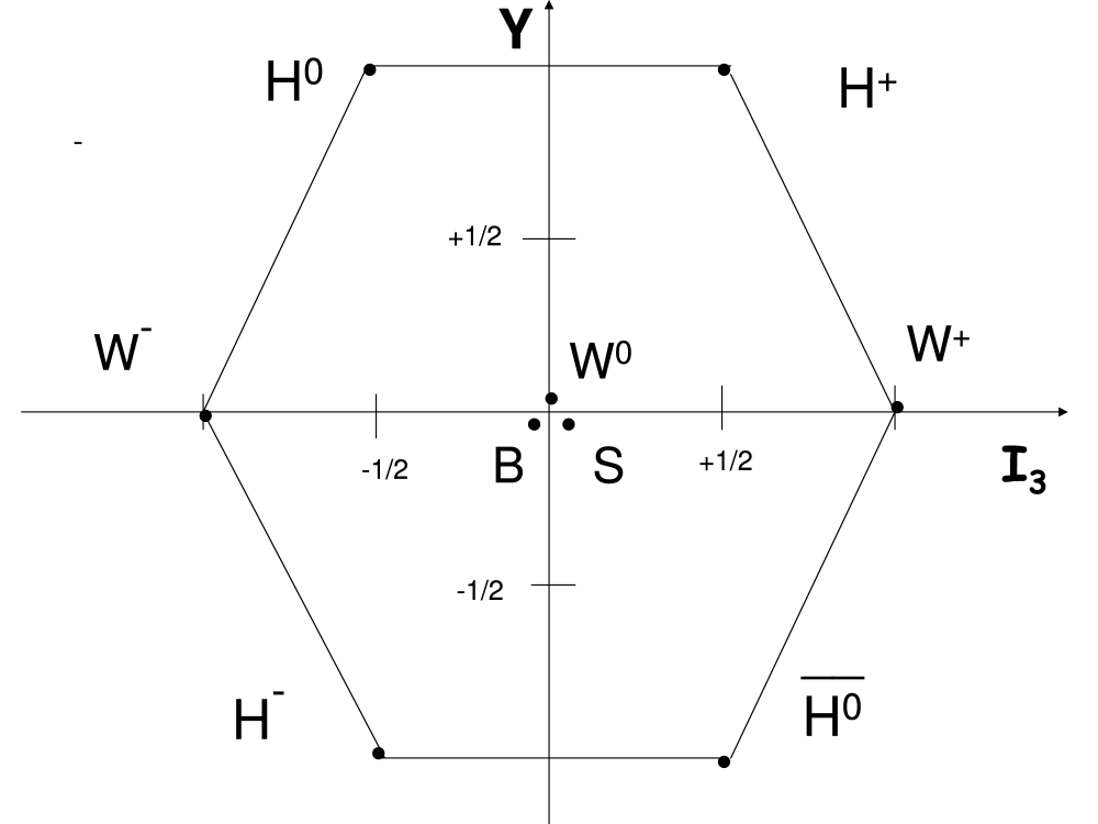
Figure 1: Fields to be associated with the regular octet and singlet representation of electroweak SU(3). $Y$ and $I_{3}$ are the electroweak quantum numbers of the fields derived from those of their ’constituents’, see Table 1.

The same signs for the hypercharge currents interacting with the $B$- field shall be needed in order to obtain the correct signs for the electric charge currents interacting with the $A$-field, i.e. the photon, as will be shown below. This can be achieved mixing (by field rotation) the isoscalar octet member $B_{8}$ with the singlet $S$ as a first step. Thus, the singlet field and corresponding current play a role in the present approach whereas it is discarded in the SM of electroweak interactions as it is in the Standard Model of the strong interaction, QCD.

The next step after this rotation from $B_{8}$ and $S$ to $B$ and $S^{\prime}$ corresponds to the familiar standard mixing, i.e. rotation by the Weinberg angle of the resulting $B$ field and of the $W^{0}$-field in order to obtain the $A$- and $Z$-boson.

In the following, firstly the case of leptons is considered. An attempt is made to derive both vector and scalar fields from a common local gauge symmetry. This will require a somewhat different formulation of the Dirac equation. The assumed SU(3) symmetry determines the Weinberg angle. It is shown, that the same value of the Weinberg angle emerges in the SM, too, if the world would consist only of the known leptons. This is a consequence of the choice of the hypercharge current attached to the U(1) symmetry of the SM.

Subsequently, the SU(3) symmetry is extended to quarks. It turns out that the Han-Nambu scheme [6] explaining the fractional charges of quarks as averages of three integer quark charges allows a straight-forward extension of the SU(3) symmetry to electroweak quark interactions.

2 SU(3) Invariant Lagrangian for Leptons

The basic Dirac field operators describing the leptons are 4-component bispinors, $\psi$ and expressed as column vector: The adjoint bispinors are defined as $\bar{\psi}=\psi^{\dagger}\gamma^{0}$ and row vectors.

The following covariant bilinear products, of the bispinors and their adjoints, with 4x4 Dirac matrices, $\gamma^{\mu}$, where $\mu=0,1,2,3$ and their product $\gamma^{5}=i\gamma^{0}\gamma^{1}\gamma^{2}\gamma^{3}$, have specific behaviour (scalar, vector etc) under Lorentz transformations (boosts), rotations and space inversion:

$\bar{\psi}\cdot\psi\;\;\;\;\;\;$ scalar

$\bar{\psi}\cdot\gamma^{5}\cdot\psi\;\;\;\;\;\;$ pseudoscalar

$\bar{\psi}\cdot\gamma^{\mu}\cdot\psi\;\;\;\;\;\;$ vector

$\bar{\psi}\cdot\gamma^{\mu}\cdot\gamma^{5}\cdot\psi\;\;\;\;\;\;$ axial vector

The chirality projections, right (R) and left (L) handed bispinors, are obtained by multiplication of the bispinor with the corresponding projection operators:

$\psi_{R}=\tfrac{1}{2}(1+\gamma^{5})\cdot\psi\;\;\;\;\;\;$ and $\;\;\;\;\;\;\psi_{L}=\tfrac{1}{2}(1-\gamma^{5})\cdot\psi$

Some properties of covariant bilinear products of chiral projections, which are relevant for the present approach are summarized here:

$\overline{\psi}\cdot\psi_{R}=\overline{\psi_{L}}\cdot\psi_{R},\;\;\;\;$ $\overline{\psi}\cdot\psi_{L}=\overline{\psi_{R}}\cdot\psi_{L},\;\;\;\;$ $\overline{\psi}\cdot\gamma^{5}\cdot\psi_{R}=\overline{\psi_{L}}\cdot\gamma^{5}\cdot\psi_{R}\;\;\;\;$ $\overline{\psi}\cdot\gamma^{5}\cdot\psi_{L}=\overline{\psi_{R}}\cdot\gamma^{5}\cdot\psi_{L}$

$\overline{\psi}\cdot\gamma^{\mu}(\cdot\gamma^{5})\cdot\psi_{R}=\overline{\psi_{R}}\cdot\gamma^{\mu}(\cdot\gamma^{5})\cdot\psi_{R}\;\;\;$ and $\overline{\psi}\cdot\gamma^{\mu}(\cdot\gamma^{5})\cdot\psi_{L}=\overline{\psi_{L}}\cdot\gamma^{\mu}(\cdot\gamma^{5})\cdot\psi_{L}$

In particular, the chiral projections turn out to be orthogonal to their own adjoints in the scalar and pseudoscalar product, i.e. the scalar ($1$) and pseudoscalar ($\gamma^{5}$) operators flip the chirality, whereas in case of the vector and axial vector currents the chirality is conserved and opposite chiralities are orthogonal:

$\overline{\psi_{R}}\cdot{\psi_{R}}=\overline{\psi_{L}}\cdot\psi_{L}=\overline{\psi_{R}}\cdot\gamma^{5}\cdot\psi_{R}=\overline{\psi_{L}}\cdot\gamma^{5}\cdot\psi_{L}=0\;\;\;\;\;\;\;\;\;\;\;\;\;\;\;\;\;\;\;\;\;\;\;\;\;\;\;\;\;\;\;\;\;\;\;\;\;\;\;\;$ (1)

$\overline{\psi_{R}}\cdot\gamma^{\mu}\cdot\psi_{L}=\overline{\psi_{L}}\cdot\gamma^{\mu}\cdot\psi_{R}=\overline{\psi_{R}}\cdot\gamma^{\mu}\cdot\gamma^{5}\cdot\psi_{L}=\overline{\psi_{L}}\cdot\gamma^{\mu}\cdot\gamma^{5}\cdot\psi_{R}=0\;\;\;\;\;\;\;\;\;\;\;\;\;\;$ (2)

The heuristic approach towards an SU(3) based electroweak interaction model for leptons outlined in the introduction has shown that scalar fields and vector fields play a complementary role in the nine fields coupling to the basic triplet of leptons. Thus a major challenge for the present approach has been to justify the emergence of scalar fields in addition to vector fields. The solution is as follows and first explained for the simpler case of U(1) and SU(2) symmetries if one considers a world of electrons only. The Lagrangian leading to the free Dirac equation via the Euler Lagrange equation is

$$\mathcal{L}=i\bar{\psi}\partial_{\mu}\gamma^{\mu}\psi-\bar{\psi}m\psi\;\;\;\;\;\;\;\;\;\;\;\;\;\;\;\;\;\;\;\;\;\;\;\;\;\;\;\;\;\;\;\;\;\;\;\;\;\;\;\;\;\;\;\;\;\;\;\;\;\;\;\;\;\;\;\;\;\;\;\;\;\;\;\;\;\;\;\;\;\;\;\;\;\;\;\;$$

Gauge symmetry under the U(1) transformations

$U=e^{ie\alpha(x)}\;\;\;\;\;\;$ so that $\;\;\;\psi(x)\rightarrow e^{ie\alpha(x)}\psi(x)\;\;\;\;\;\;$ and $\;\;\;\overline{\psi(x)}\rightarrow e^{-ie\alpha(x)}\overline{\psi(x)}$

requires the existence of a vector field potential $A_{\mu}$ (naturally to be associated with the photon). This field must transform under U(1) transformations as:

$A_{\mu}\rightarrow A_{\mu}+\partial_{\mu}\alpha(x)$

It is proposed to rewrite the free Dirac Lagrangian in the following way:

$$\mathcal{L}=i\bar{\psi}\partial_{\mu}\gamma^{\mu}\psi-i\bar{\psi}d_{\tau}\psi\;\;\;\;\;\;\;\;\;\;\;\;\;\;\;\;\;\;\;\;\;\;\;\;\;\;\;\;\;\;\;\;\;\;\;\;\;\;\;\;\;\;\;\;\;\;\;\;\;\;\;\;\;\;\;\;\;\;\;\;\;\;\;\;\;\;\;\;\;\;\;\;\;\;\;\;\;\;\;\;\;\;\;\;\;\;\;\;\;(3)$$

where the derivative replacing the mass m in the standard Lagrangian, $id_{\tau}=id/d\tau=iu^{\mu}\partial_{\mu}$, is taken with respect to the eigentime $\tau$ of the lepton and $u^{\mu}$ is the four-velocity of the lepton. It implements the correspondence between classic particle 4-momentum and quantum operators $p_{\mu}\rightarrow i\partial_{\mu}$ by

$m\rightarrow id_{\tau}:=iu^{\mu}\partial_{\mu}$

With this modification, invariance under the above unitary transformation U requires the addition of the scalar product of the vector field potential to the lepton 4-velocity $A=u^{\mu}A_{\mu}$. This may be interpreted as an effectively scalar field. The Lagrangian becomes, with the standard definition and coupling of the photon field $A_{\mu}$ and the standard replacement of the covariant derivative $\partial_{\mu}$ by $D_{\mu}=\partial_{\mu}-ieA_{\mu}$:

$$\mathcal{L}=\bar{\psi}\gamma^{\mu}(i\partial_{\mu}+eA_{\mu})\psi-\bar{\psi}u^{\mu}(i\partial_{\mu}+eA_{\mu})\psi\;\;\;\;\;\;\;\;\;\;\;\;\;\;\;\;\;\;\;\;\;\;\;\;\;\;\;\;\;\;\;\;\;\;\;\;\;\;\;\;\;\;\;\;\;\;\;\;\;\;\;\;\;\;\;\;\;\;\;\;\;\;(4)$$

This Lagrangian is invariant under the U(1) transformation defined above.

An instructive intermediate step is to extend the U(1) symmetry to SU(2), taking as a basis the two chiral projections $(e_{R},e_{L})$ of the electron defined above. This is one of the subgroups of the SU(3) considered in the present approach. Gauge symmetry with respect to the unitary transformations

$U=e^{ie\alpha_{0}(x)\cdot 1+ie\overrightarrow{\alpha}(x)\cdot\vec{\tau}}$

where $\vec{\tau}$ contains the three Pauli matrices and the $1$ behind $\alpha_{0}(x)$ is the 2x2 unity matrix, leads to two vector and two scalar fields and the covariant derivative including minimal coupling is $D_{\mu}=\partial_{\mu}-ieA^{0}_{\mu}-ie\vec{\tau}\overrightarrow{A}$. Note that here, for SU(2), the singlet representation is included by means of the first term, as it shall be done further below for SU(3). The corresponding vector potential $A^{0}_{\mu}$ can be interpreted as being the photon, since it turns out to have a purely vector coupling to the electron, i.e. couples to the vector current $\sim(\overline{e_{L}}\gamma^{\mu}e_{L}+\overline{e_{R}}\gamma^{\mu}e_{R})$. An other one associated with the phase transformations $\alpha_{3}(x)\cdot\tau_{3}$ couples to the electron like an axial vector field, i.e. to the axial current $\sim(\overline{e_{L}}\gamma^{\mu}e_{L}-\overline{e_{R}}\gamma^{\mu}e_{R})$. It is suggestive to associate it with the Z-boson. The two scalar fields emerging from the two phase changes $\alpha_{1}(x)\tau_{1}$ and $\alpha_{2}(x)\tau_{2}$ connect the left handed electron with the adjoint of the right handed electron and vice versa. These two scalar fields are the candidates to be responsible for the mass of the electron. Define the operator and its adjoint for the doublet of lepton fields by

$$\phi=\begin{pmatrix}e_{L}\\ e_{R}\end{pmatrix}\;\;\;\;\;\;\;\;\;\;\;\;\bar{\phi}=(\overline{e_{L}},\overline{e_{R}})\;\;\;\;\;\;\;\;\;\;\;\;\;\;\;\;\;\;\;\;\;\;\;\;\;\;\;\;\;\;\;\;\;\;\;\;$$

And note that the ’mass’ term of the free Lagrangian drops out: $-i\bar{\phi}d_{\tau}\phi=-i\overline{e_{R}}d_{\tau}e_{R}-i\overline{e_{L}}d_{\tau}e_{L}=0$ owing to the orthogonality of the chirality eigenstates with their adjoints, see equation (1). But the mass term is replaced by the two interaction terms with the scalar fields: $-e\bar{\phi}u^{\mu}(\tau_{1}A_{\mu}^{1}+\tau_{2}A_{\mu}^{2})\phi$. The effectively scalar fields may serve for the mass generation by spontaneous symmetry breaking.

The SU(2) symmetry of the SM corresponds to another subgroup of SU(3). The basic leptons are the two left handed particles, $\nu_{L},e_{L}$. Four vector fields -and no scalar field emerge if one includes phase transformation $\alpha_{0}(x)$ as for the SU(2) above. The corresponding current corresponding to the singlet representation is $J^{\mu}_{0}\;\sim\;(\bar{\nu_{L}}\gamma^{\mu}\nu_{L}+\bar{e_{L}}\gamma^{\mu}e_{L})$, which is part of the current introduced through U(1) of the SM. In other words, the Standard Model does not directly include this term but the separate U(1) symmetry with respect to the hypercharge current $J^{\mu}_{Y}\sim(J^{\mu}_{0}+2\bar{e_{R}}\gamma^{\mu}e_{R})$ contains part of it. The three vector fields required by SU(2) of the SM and SU(2) subgroup of the presented SU(3) model are the $W$ bosons. The vector field associated with the U(1) symmetry and the current $J^{\mu}_{Y}$ of the SM is the $B$ boson.

In the present work the basic triplet of SU(3) consists of the leptons. They are contained in the column three vector called $\phi$ and its adjoint:

$$\phi=\begin{pmatrix}\nu_{L}\\ e_{L}\\ e_{R}\end{pmatrix}\;\;\;\;\;\;\;\;\;\;\;\;\bar{\phi}=(\overline{\nu_{L}},\overline{e_{L}},\overline{e_{R}})\;\;\;\;\;\;\;\;\;\;\;\;\;\;\;\;\;\;\;\;\;\;\;\;\;\;\;\;\;\;\;\;\;\;\;\;$$

The free Lagrangian is obtained from the Lagrangian, see equation (3), replacing the single Dirac field operator $\psi$ by the 3- vector of Dirac field operators $\phi$. SU(3) gauge symmetry is assumed, i.e. invariance of the Lagrangian with respect to the special unitary transformation

$\;\;\;\;\;\;\;\;U=e^{ig\overrightarrow{\alpha}(x)\cdot\vec{\lambda}}\;\;\;\;\;\;\;\;\;\;\;\;\;\;\;\;\;\;\;\;\;\;\;\;\;\;\;\;\;\;\;\;\;\;\;\;\;\;\;\;\;\;\;\;\;\;\;\;\;\;\;\;\;\;\;\;\;\;\;\;\;\;\;\;\;\;\;\;\;\;\;\;\;\;\;\;\;\;\;\;\;\;\;\;\;\;\;\;\;\;\;\;\;\;\;\;(5)$

The 9-vector $\vec{\lambda}=(\lambda_{0},\lambda_{1},...,\lambda_{8})$ contains the standard Gell-Mann matrices ($\lambda_{1},...,\lambda_{8}$) implemented by the unity matrix $\lambda_{0}=1\cdot\sqrt{2/3}$ needed for the SU(3) singlet term. (The factor $\sqrt{2/3}$ has to be applied in order to have the same normalisation as the other matrices.) Requiring gauge symmetry with respect to U and minimal coupling will lead to interaction terms with vector and scalar fields, depending on the combination of left and right handed leptons as dictated by the $\lambda$ matrices. The initial names to be used for the nine fields to be expected are $X_{\mu}^{0},...,X_{\mu}^{8}$. The Lagrangian implemented by the interaction term (but not yet including the field energy density terms) is now:

$$\mathcal{L}=\bar{\phi}\gamma^{\mu}(i\partial_{\mu}+g\vec{\lambda}\vec{X}_{\mu})\phi-\bar{\phi}u^{\mu}(i\partial_{\mu}+g\vec{\lambda}\vec{X}_{\mu})\phi=\bar{\phi}\gamma^{\mu}i\partial_{\mu}\phi+g\bar{\phi}(\gamma^{\mu}-u^{\mu})\vec{\lambda}\vec{X}_{\mu}\phi\;\;\;\;\;\;\;\;\;\;(6)$$

This Lagrangian is invariant under the SU(3) transformations (5). Due to the orthogonality properties, see equations (2), of the chiral projections, the term $-\bar{\phi}u^{\mu}(i\partial_{\mu})\phi$ of the free Lagrangian has dropped out for the present choice of the basic triplet- as it already did for the extensions to SU(2). Thus the masses have to arise from the interaction of the leptons with the effectively scalar fields $u^{\mu}\vec{\lambda}\vec{X}_{\mu}$.

The interaction term written as an explicit sum is

$g\bar{\phi}(\gamma^{\mu}-u^{\mu})\vec{\lambda}\overrightarrow{X_{\mu}}\phi=\sum_{i=0,.,9}g\bar{\phi}(\gamma^{\mu}-u^{\mu})\lambda_{i}X_{\mu}^{i}\phi=:\sum_{i=0,.,9}\Lambda_{i}\;\;\;\;\;\;\;\;\;\;\;\;\;\;\;\;\;\;\;\;\;\;\;\;\;\;\;(7)$

Considering the vector current interaction terms, $\Lambda_{i}=g\cdot\bar{\phi}\cdot\gamma^{\mu}\cdot\lambda_{i}\cdot X_{\mu}^{i}\cdot\phi$, it is obvious from the orthogonality relations (2) that only five of them survive, namely those with chirality conserving currents. For the scalar interaction terms, $\Lambda_{i}=g\cdot\bar{\phi}\cdot u^{\mu}\cdot\lambda_{i}\cdot X_{\mu}^{i}\cdot\phi$, the other four with chirality changing currents survive. The complete list is:

$\Lambda_{0}=g\cdot(\overline{\nu_{L}}\gamma^{\mu}\nu_{L}+\overline{e_{L}}\gamma^{\mu}e_{L}+\overline{e_{R}}\gamma^{\mu}e_{R})\cdot X_{\mu}^{0}\cdot\sqrt{2/3}$
$\Lambda_{1}=g\cdot(\overline{\nu_{L}}\gamma^{\mu}e_{L}+\overline{e_{L}}\gamma^{\mu}\nu_{L})\cdot X_{\mu}^{1}$
$\Lambda_{2}=g\cdot(-i\overline{\nu_{L}}\gamma^{\mu}e_{L}+i\overline{e_{L}}\gamma^{\mu}\nu_{L})\cdot X_{\mu}^{2}$
$\Lambda_{3}=g\cdot(\overline{\nu_{L}}\gamma^{\mu}\nu_{L}-\overline{e_{L}}\gamma^{\mu}e_{L})\cdot X_{\mu}^{3}$
$\Lambda_{4}=g\cdot(\overline{\nu_{L}}u^{\mu}e_{R}+\overline{e_{R}}u^{\mu}\nu_{L})\cdot X_{\mu}^{4}\;\;\;\;\;\;\;\;\;\;\;\;\;\;\;\;\;\;\;\;\;\;\;\;\;\;\;\;\;\;\;\;\;\;\;\;\;\;\;\;\;\;\;\;\;\;\;\;\;\;\;\;\;\;\;\;\;\;\;\;\;\;\;\;\;\;\;\;\;\;\;\;\;\;\;\;\;\;\;\;(8)$
$\Lambda_{5}=g\cdot(-i\overline{\nu_{L}}u^{\mu}e_{R}+i\overline{e_{R}}u^{\mu}\nu_{L})\cdot X_{\mu}^{5}$
$\Lambda_{6}=g\cdot(\overline{e_{L}}u^{\mu}e_{R}+\overline{e_{R}}u^{\mu}e_{L})\cdot X_{\mu}^{6}$
$\Lambda_{7}=g\cdot(-i\overline{e_{L}}u^{\mu}e_{R}+i\overline{e_{R}}u^{\mu}e_{L})\cdot X_{\mu}^{7}$
$\Lambda_{8}=g\cdot(\overline{\nu_{L}}\gamma^{\mu}\nu_{L}+\overline{e_{L}}\gamma^{\mu}e_{L}-2\overline{e_{R}}\gamma^{\mu}e_{R})\cdot X_{\mu}^{8}/\sqrt{3}$

The interaction terms will be discussed in the following with a focus on the comparison with the SM and on the determination of the Weinberg angle.

3 Comparison of Interaction Terms

Recomposing the first two terms by replacement of $\lambda_{1},\lambda_{2}$ and $X_{\mu}^{1},X_{\mu}^{2}$ with $\lambda_{1\pm 2}=\lambda_{1}\pm i\lambda_{2}$ and $X_{\mu}^{1\pm 2}=(X_{\mu}^{1}\pm iX_{\mu}^{2})/\sqrt{2}$ the sum of the first two terms $\Lambda_{1},\Lambda_{2}$ is transformed into a new sum $\Lambda_{1+2}+\Lambda_{1-2}=\Lambda_{1}+\Lambda_{2}$ with:

$\Lambda_{1+2}=(g/\sqrt{2})\cdot\bar{\phi}\cdot\lambda_{1+2}\cdot\gamma^{\mu}\cdot\phi\cdot X_{\mu}^{1-2}=(\sqrt{2}g)\cdot\overline{\nu_{L}}\gamma^{\mu}e_{L}\cdot X_{\mu}^{1-2}$
$\Lambda_{1-2}=(g/\sqrt{2})\cdot\bar{\phi}\cdot\lambda_{1-2}\cdot\gamma^{\mu}\cdot\phi\cdot X_{\mu}^{1+2}=(\sqrt{2}g)\cdot\overline{e_{L}}\gamma^{\mu}\nu_{L}\cdot X_{\mu}^{1+2}$

Next, it is shown that the three terms $\Lambda_{1+2},\Lambda_{1-2},\Lambda_{3}$ are proportional to the interaction terms of the weak charged and neutral currents with the W- bosons of the SU(2) part of the Standard Model (SM). This is to be expected since the matrices $\lambda_{1},\lambda_{2},\lambda_{3}$ project the electroweak lefthanded lepton doublet out of the present triplet and their effective part is a copy of the Pauli matrices $\tau_{1},\tau_{2},\tau_{3}$.

The interaction term of the SM Lagrangian for the SU(2) symmetric part is, before the rotation by the Weinberg angle,

$\Lambda_{SU(2)}^{SM}=g_{SM}\cdot\overline{\chi_{L}}\cdot\gamma^{\mu}\cdot\vec{T}\cdot\overrightarrow{W_{\mu}}\cdot\chi_{L}$ $=g_{SM}\overrightarrow{J^{\mu}}\overrightarrow{W_{\mu}}$

Here, $\chi_{L}$ is the column vector of the (weak isospin) doublet of the two left-handed bispinors associated with $\nu_{L}$ and $e_{L}$ and $\overline{\chi_{L}}$ is the row vector adjoint to $\chi_{L}$:

$$\chi_{L}=\begin{pmatrix}\nu_{L}\\ e_{L}\end{pmatrix}\;\;\;\;\;\;\;\;\;\;\;\;\overline{\chi_{L}}=(\overline{\nu_{L}},\overline{e_{L}})$$

The 3-component vector $\vec{T}=\vec{\tau}/2$ contains the three generators of weak isospin. The vector $\overrightarrow{W_{\mu}}$ represents the three associated vector fields. The three weak isospin currents $\overrightarrow{J^{\mu}}$ contained in the SU(2) interaction term above are:

$[J^{\mu}_{1},J^{\mu}_{2},J^{\mu}_{3}]=\tfrac{1}{2}[(\overline{\nu_{L}}\gamma^{\mu}e_{L}+\overline{e_{L}}\gamma^{\mu}\nu_{L}),(-i\overline{\nu_{L}}\gamma^{\mu}e_{L}+i\overline{e_{L}}\gamma^{\mu}\nu_{L}),(\overline{\nu_{L}}\gamma^{\mu}\nu_{L}-\overline{e_{L}}\gamma^{\mu}e_{L})]$

In the SM, the first two interaction terms are recomposed into two charged current interactions, as in the present approach, which was guided by the SM. The two charged currents are:

$J^{\mu}_{+}:=J^{\mu}_{1}+iJ^{\mu}_{2}=\overline{\nu_{L}}\gamma^{\mu}e_{L}\;\;\;\;\;\;\;\;\;\;\;\;\;\;$ and $\;\;\;\;\;\;\;\;\;\;\;\;\;\;\;\;\;\;\;\;J^{\mu}_{-}:=J^{\mu}_{1}-iJ^{\mu}_{2}=\overline{e_{L}}\gamma^{\mu}\nu_{L}$

The two associated charged fields are defined as were the fields $X_{\mu}^{1-2},X_{\mu}^{1+2}$:

$W_{\mu}^{+}=\tfrac{1}{\sqrt{2}}(W_{\mu}^{1}-iW_{\mu}^{2})\;\;\;\;\;\;\;\;\;\;\;\;\;\;\;\;\;\;\;\;$ and $\;\;\;\;\;\;\;\;\;\;\;\;\;\;\;\;\;\;\;\;W_{\mu}^{-}=\tfrac{1}{\sqrt{2}}(W_{\mu}^{1}+iW_{\mu}^{2})$

Now, it is obvious that the three interaction terms of SU(2) of the SM:

$[\Lambda_{-}^{SM},\;\Lambda_{+}^{SM},\;\Lambda_{3}^{SM}]$ $=g_{SM}[\tfrac{1}{\sqrt{2}}\overline{\nu_{L}}\gamma^{\mu}e_{L}W_{\mu}^{+},\;\tfrac{1}{\sqrt{2}}\overline{e_{L}}\gamma^{\mu}\nu_{L}W_{\mu}^{-},\;\tfrac{1}{2}(\overline{\nu_{L}}\gamma^{\mu}\nu_{L}-\overline{e_{L}}\gamma^{\mu}e_{L})W_{\mu}^{0}]$

and those of the present SU(3) approach, $\Lambda_{1+2},\Lambda_{1-2},\Lambda_{3}$, are consistent, apart from the fact that the coupling constants are differently defined in the SM. (There is a factor 2 between the two definitions. This can be traced back to the different normalisations of the $T$ used in the SM and of the $\lambda$ matrices used here for SU(3) transformations, equation (5).)

The interaction term for the U(1) part of the SM describes the interaction of a weak hypercharge current with a vector field called $B_{\mu}$. The hypercharge current of the SM is due to the weak hypercharge $Y=2(Q-I_{3})$ and is therefore defined as:

$J^{\mu}_{Y}=2J^{\mu}_{e.m.}-2J^{\mu}_{3}=(-2)(\overline{e_{L}}\gamma^{\mu}e_{L}+\overline{e_{R}}\gamma^{\mu}e_{R})-2\cdot\tfrac{1}{2}(\overline{\nu_{L}}\gamma^{\mu}\nu_{L}-\overline{e_{L}}\gamma^{\mu}e_{L})$

The corresponding interaction term is:

$\Lambda_{U(1)}^{SM}=\tfrac{g^{\prime}_{SM}}{2}J_{Y}^{\mu}B_{\mu}=\tfrac{g^{\prime}_{SM}}{2}(-\overline{\nu_{L}}\gamma^{\mu}\nu_{L}-\overline{e_{L}}\gamma^{\mu}e_{L}-2\overline{e_{R}}\gamma^{\mu}e_{R})B_{\mu}$

The term $\Lambda_{U(1)}^{SM}$ resembles the term $\Lambda_{8}$. However, as already mentioned, the relative signs in $\Lambda_{8}$ do not correspond to those in $\Lambda_{U(1)}^{SM}$. An unavoidable consequence is that after mixing of the hypercharge candidate vector field $X_{\mu}^{8}$ with $X_{\mu}^{3}=W_{\mu}^{0}$ in order to obtain the photon field (coupling only to the electron), the left handed and right handed electron currents have opposite sign instead of the same signs as needed for a pure vector interaction.

(One may try to cure the problem of the signs of terms in the SU(3) hypercharge current by choosing as third member of the fundamental triplet instead of the $e_{R}$ the charge conjugate of the right-handed electron, a left handed positron. This solves the problem of signs. But causes other problems difficult to solve. Thus another path has been chosen to obtain the correct signs for the terms in the hypercharge current.)

So far, the singlet combination $\Lambda_{0}$ of the nonet, see above, has been left aside. It shall be mixed with the interaction $\Lambda_{8}$ in order to obtain the weak hypercharge interaction, where the new field $X_{\mu}^{8^{\prime}}$ corresponds to the $B_{\mu}$- field of the SM so that the interaction becomes:

$\Lambda_{8}^{\prime}=\tfrac{g}{\sqrt{3}}(-\overline{\nu_{L}}\gamma^{\mu}\nu_{L}-\overline{e_{L}}\gamma^{\mu}e_{L}-2\overline{e_{R}}\gamma^{\mu}e_{R})\cdot X_{\mu}^{8^{\prime}}$

This implies rotating the fields and currents by an angle $\alpha$.

$$\begin{pmatrix}X_{\mu}^{8}\\ X_{\mu}^{0}\end{pmatrix}=\begin{pmatrix}cos\alpha&sin\alpha\\ -sin\alpha&cos\alpha\end{pmatrix}\cdot\begin{pmatrix}X_{\mu}^{8^{\prime}}\\ X_{\mu}^{0^{\prime}}\end{pmatrix}$$

In order to obtain the wanted interaction term $\Lambda_{8}^{\prime}$ the equation to be solved is

$\Lambda_{0}+\Lambda_{8}=$

$=\tfrac{\sqrt{2}g}{\sqrt{3}}(\overline{\nu_{L}}\gamma^{\mu}\nu_{L}+\overline{e_{L}}\gamma^{\mu}e_{L}+\overline{e_{R}}\gamma^{\mu}e_{R})\cdot(cos\alpha\cdot X_{\mu}^{0^{\prime}}-sin\alpha\cdot X_{\mu}^{8^{\prime}}$

$+\tfrac{g}{\sqrt{3}}(\overline{\nu_{L}}\gamma^{\mu}\nu_{L}+\overline{e_{L}}\gamma^{\mu}e_{L}-2\overline{e_{R}}\gamma^{\mu}e_{R})\cdot(cos\alpha\cdot X_{\mu}^{8^{\prime}}+sin\alpha\cdot X_{\mu}^{0^{\prime}})\;\;\;\;\;\;\;\;\;\;\;\;\;\;\;\;\;\;\;\;\;\;\;\;(9)$
$=\Lambda_{0}^{\prime}+\Lambda_{8}^{\prime}=$

$=\tfrac{\sqrt{2}g}{\sqrt{3}}J^{\mu}_{0^{\prime}}\cdot X_{\mu}^{0^{\prime}}+\tfrac{g}{\sqrt{3}}(-\overline{\nu_{L}}\gamma^{\mu}\nu_{L}-\overline{e_{L}}\gamma^{\mu}e_{L}-2\overline{e_{R}}\gamma^{\mu}e_{R})\cdot X_{\mu}^{8^{\prime}}$

The solution of equation (9) is given by $cos\alpha=1/3$ and $sin\alpha=\sqrt{8/9}$.

The new interaction terms are:

$\Lambda_{8}^{\prime}=\tfrac{g}{\sqrt{3}}(-\overline{\nu_{L}}\gamma^{\mu}\nu_{L}-\overline{e_{L}}\gamma^{\mu}e_{L}-2\overline{e_{R}}\gamma^{\mu}e_{R})\cdot X_{\mu}^{8^{\prime}}$

$\Lambda_{0}^{\prime}=\tfrac{\sqrt{2}g}{\sqrt{3}}(\overline{\nu_{L}}\gamma^{\mu}\nu_{L}+\overline{e_{L}}\gamma^{\mu}e_{L}-\overline{e_{R}}\gamma^{\mu}e_{R})\cdot X_{\mu}^{{}^{\prime}0}\;\;\;\;\;\;\;\;\;\;\;\;\;\;\;\;\;\;\;\;\;\;\;\;\;\;\;\;\;\;\;\;\;\;\;\;\;\;\;\;\;\;\;\;\;\;\;\;(10)$

Thus, $\Lambda_{8}^{\prime}$ becomes proportional to $\Lambda_{U(1)}^{SM}$. The field $X_{\mu}^{8^{\prime}}$ can be identified with $B_{\mu}$- field of $\Lambda_{U(1)}^{SM}$.

Four of the nine independent boson fields entering the sum of interaction terms, equation (8), enter as projections onto the four-velocity of the leptons ($u^{\mu}\cdot X_{mu}^{i},\;\;i=4-7$). These projections behave effectively like scalar fields. In the following, they shall be treated like scalar fields with the names $X^{4},X^{5},X^{6},X^{7}$, in order to show their relation to the scalar fields of the SM.

Firstly, the four interaction terms $\Lambda_{4}$ to $\Lambda_{7}$ shall be recomposed as it was done for the terms $\Lambda_{1},\Lambda_{2}$. Defining $\lambda_{4\pm 5}=\lambda_{4}\pm i\lambda_{5}$ and $X^{4\pm 5}=(X^{4}\pm iX^{5})/\sqrt{2}$ and correspondingly for the indices 6,7 one obtains:

$\Lambda_{4+5}=(g/\sqrt{2})\cdot\bar{\phi}\cdot\lambda_{4+5}\cdot\phi\cdot X^{4-5}=(\sqrt{2}g)\cdot\overline{\nu_{L}}e_{R}\cdot X^{4-5}$
$\Lambda_{4-5}=(g/\sqrt{2})\cdot\bar{\phi}\cdot\lambda_{4-5}\cdot\phi\cdot X^{4+5}=(\sqrt{2}g)\cdot\overline{e_{R}}\nu_{L}\cdot X^{4+5}$
$\Lambda_{6+7}=(g/\sqrt{2})\cdot\bar{\phi}\cdot\lambda_{6+7}\cdot\phi\cdot X^{6-7}=(\sqrt{2}g)\cdot\overline{e_{L}}e_{R}\cdot X^{6-7}$
$\Lambda_{6-7}=(g/\sqrt{2})\cdot\bar{\phi}\cdot\lambda_{6-7}\cdot\phi\cdot X^{6+7}=(\sqrt{2}g)\cdot\overline{e_{R}}e_{L}\cdot X^{6+7}$

The four resulting fields can be identified with the four independent fields associated with the complex isospin doublet of the SM: With

$$\Phi=\begin{pmatrix}\Phi^{+}\\ \Phi^{0}\end{pmatrix}\;\;\;\;\;\;\;\;\;\;\;\;\Phi^{{\dagger}}=(\Phi^{+*},\Phi^{0*})$$

the four corresponding interaction terms of the SM are

$f_{e}(\overline{\chi_{L}}e_{R}\Phi+\overline{e_{R}}\chi_{L}\Phi^{{\dagger}})=f_{e}(\overline{\nu_{L}}e_{R}\cdot\Phi^{+}+\overline{e_{L}}e_{R}\cdot\Phi^{0}+\overline{e_{R}}\nu_{L}\cdot\Phi^{+*}+\overline{e_{R}}e_{L}\cdot\Phi^{0*})$

Thus, the identifications $X^{4-5}=\Phi^{+}$, $X^{4+5}=\Phi^{+*}$, $X^{6-7}=\Phi^{0}$ and $X^{6+7}=\Phi^{0*}$ are obvious. The coupling constant $f_{e}$ is another independent constant of the SM. In the present approach these coupling constants are determined by the SU(3) symmetry.

4 Rotation towards Light

After having obtained an interaction term corresponding to that of the Standard Model (SM) for the hypercharge current interaction with the $B$ field, the next rotation aims to obtain the field $A_{\mu}$ corresponding to the photon which couples only to the charged leptons $e_{R},e_{L}$, more precisley to $J^{\mu}_{e.m.}=-(\overline{e_{L}}\gamma^{\mu}e_{L}+\overline{e_{R}}\gamma^{\mu}e_{R})$ and the new Z boson field $Z_{\mu}$, by mixing $B_{\mu}$ and $W_{\mu}^{0}$. This rotation is described by the Weinberg angle.

For the considerations in the following section it is useful to define ’bare’ currents, where no quantum number factors are included. In particular, the three possible bare neutral currents are:

$\overrightarrow{j^{\mu}}=(j^{\mu}_{1},j^{\mu}_{2},j^{\mu}_{3})=(\overline{\nu_{L}}\gamma^{\mu}\nu_{L},\;\;\overline{e_{L}}\gamma^{\mu}e_{L},\;\;\overline{e_{R}}\gamma^{\mu}e_{R}$ )

The neutral currents of the SM can then be rewritten as products of a 3-vector of quantum numbers with the three- vector of these bare currents:

$J^{\mu}_{3}=\sum I_{3_{i}}j^{\mu}_{i}=\overrightarrow{I_{3}}\cdot\overrightarrow{j^{\mu}}$ with $\overrightarrow{I_{3}}=(\tfrac{1}{2},-\tfrac{1}{2},0)$

$J^{\mu}_{Y}=\sum Y_{i}j^{\mu}_{i}=\overrightarrow{Y}\cdot\overrightarrow{j^{\mu}}$ with $\overrightarrow{Y}=(-1,-1,-2)$

$J^{\mu}_{e.m.}=\sum Q_{i}j^{\mu}_{i}=\overrightarrow{Q}\cdot\overrightarrow{j^{\mu}}$ with $\overrightarrow{Q}=(0,-1,-1)$

The vectors $\overrightarrow{I_{3}}$ and $\overrightarrow{Y}$, as they have been derived based on SU(3), are, of course, identical to the vectors of diagonal elements of the generators $\lambda_{3}$ and $\lambda^{\prime}_{8}$ of the group SU(3), apart from a normalization factor. These 3-vectors are orthogonal:

$\overrightarrow{I_{3}}\cdot\overrightarrow{Y}=0$

They are also orthogonal to the vector of quantum numbers of the third neutral current corresponding to the singlet interaction $\Lambda^{\prime}_{0}$. The currents $J^{\mu}_{3}$ and $J^{\mu}_{Y}$ are orthogonal in the SM, too. There, it is due to the choice of the hypercharge currents for the U(1) part of the SU(2)xU(1) symmetry.

For a more general approach and in order to facilitate the comparison with the SM, an SU(3) symmetry breaking shall be introduced, or in other words, an additional freedom by allowing the $X_{\mu}^{8^{\prime}}$ field to have a different coupling constant ($g^{\prime}$) from the coupling ($g$) of $X_{\mu}^{3}$. Thus the two interaction terms are now, identifying $X_{\mu}^{8^{\prime}}$ with $B_{\mu}$ and $X_{\mu}^{3}$ with $W_{\mu}^{0}$ of the SM:

$\Lambda_{3}=g(\overline{\nu_{L}}\gamma^{\mu}\nu_{L}-\overline{e_{L}}\gamma^{\mu}e_{L})W_{\mu}^{0}=2g\overrightarrow{I_{3}}\cdot\overrightarrow{j^{\mu}}W_{\mu}^{0}$

$\Lambda^{\prime}_{8}=\tfrac{g^{\prime}}{\sqrt{3}}(-\overline{\nu_{L}}\gamma^{\mu}\nu_{L}-\overline{e_{L}}\gamma^{\mu}e_{L}-2\overline{e_{R}}\gamma^{\mu}e_{R})B_{\mu}=\tfrac{g^{\prime}}{\sqrt{3}}\overrightarrow{Y}\cdot\overrightarrow{j^{\mu}}B_{\mu}$

which are identical to the two interaction terms ($\Lambda_{3},\Lambda^{\prime}_{8}$) obtained above, except of the different coupling $g^{\prime}$ assumed for the second term. They coincide with the neutral interaction terms of the Standard Model, apart from the already mentioned factor 2 owing to different definitions of currents or couplings. The goal of rotating the above fields and currents is to obtain the correct photon $A$ interaction with the charged lepton, the electron: a purely vector interaction. The remaining, orthogonal part of the currents will couple to the other field ($Z$) orthogonal to $A$ obtained after rotation:

$\Lambda_{A}:=-e\cdot(\overline{e_{L}}\gamma^{\mu}e_{L}+\overline{e_{R}}\gamma^{\mu}e_{R})\cdot A_{\mu}=eJ_{e.m.}^{\mu}A_{\mu}=e\cdot\overrightarrow{Q}\cdot\overrightarrow{j^{\mu}}$

$\Lambda_{Z}=g_{Z}J_{Z}^{\mu}Z_{\mu}$

where e is the absolute electric charge of the electron, $e=1.6....\cdot 10^{-19}C$, and $g_{Z}$ and $J_{Z}^{\mu}$ will be determined together with the correct photon interaction. The (inverse) rotation is defined by:

$$\begin{pmatrix}B_{\mu}\\ W_{\mu}^{0}\end{pmatrix}=\begin{pmatrix}cos\theta&-sin\theta\\ +sin\theta&cos\theta\end{pmatrix}\cdot\begin{pmatrix}A_{\mu}\\ Z_{\mu}\end{pmatrix}$$

Thus, the following equation for the sum of interaction terms before and after the rotation has to be solved:

$\Lambda_{3}+\Lambda_{8}^{\prime}=g(\overline{\nu_{L}}\gamma^{\mu}\nu_{L}-\overline{e_{L}}\gamma^{\mu}e_{L})(cos\theta\cdot Z_{\mu}+sin\theta\cdot A_{\mu})$

$\;\;\;\;\;\;\;\;\;\;\;\;\;\;\;\;\;\;+\tfrac{g^{\prime}}{\sqrt{3}}(-\overline{\nu_{L}}\gamma^{\mu}\nu_{L}-\overline{e_{L}}\gamma^{\mu}e_{L}-2\overline{e_{R}}\gamma^{\mu}e_{R})(cos\theta\cdot A_{\mu}-sin\theta\cdot Z_{\mu})$

$=:-e\cdot(\overline{e_{L}}\gamma^{\mu}e_{L}+\overline{e_{R}}\gamma^{\mu}e_{R})\cdot A_{\mu}+g_{Z}\cdot J_{Z}^{\mu}\cdot Z_{\mu}=:\Lambda_{A}+\Lambda_{Z}$

The above equation leads to three constraints:

$\overline{\nu_{L}}\gamma^{\mu}\nu_{L}\cdot A_{\mu}\cdot(-cos\theta\cdot\tfrac{g^{\prime}}{\sqrt{3}}+sin\theta\cdot g)=0\;\;\;\ \;\;\;\;\;\;\ \;\;\;\;\;\;\ \;\;\;\rightarrow g^{\prime}=\sqrt{3}g\cdot tan\theta\;\;\;\;\;\;\;\;(11)$

$-2\overline{e_{R}}\gamma^{\mu}e_{R}\cdot A_{\mu}\cdot cos\theta\cdot\tfrac{g^{\prime}}{\sqrt{3}}=-e\cdot\overline{e_{R}}\gamma^{\mu}e_{R}A_{\mu}\;\;\;\;\;\;\;\;\;\;\;\;\;\;\;\rightarrow e=\tfrac{2g^{\prime}cos\theta}{\sqrt{3}}=2g\cdot sin\theta$

$\overline{e_{L}}\gamma^{\mu}e_{L}\cdot A_{\mu}(-cos\theta\cdot\tfrac{g^{\prime}}{\sqrt{3}}-sin\theta\cdot g)=-e\cdot\overline{e_{L}}\gamma^{\mu}e_{L}A_{\mu}\rightarrow e=g\cdot sin\theta+\tfrac{g^{\prime}\cdot cos\theta}{\sqrt{3}}=2g\cdot sin\theta\;$

Note, the ratios of all three coupling constants are fixed by the same angle. The new interaction terms for the photon A and the Z boson are:

$\Lambda_{A}=e(-\overline{e_{L}}\gamma^{\mu}e_{L}-\overline{e_{R}}\gamma^{\mu}e_{R})A_{\mu}=eJ_{e.m.}^{\mu}A_{\mu}\;\;\;\;\;\;\;\;\;\;\;\;\;\;\;$
$\Lambda_{Z}=g(\overline{\nu_{L}}\gamma^{\mu}\nu_{L}-\overline{e_{L}}\gamma^{\mu}e_{L})Z_{\mu}cos\theta$

$\;\;\;\;\;\;\ +\tfrac{g^{\prime}}{\sqrt{3}}(-\overline{\nu_{L}}\gamma^{\mu}\nu_{L}-\overline{e_{L}}\gamma^{\mu}e_{L}-2\overline{e_{R}}\gamma^{\mu}e_{R})(-sin\theta\cdot Z_{\mu})$

$=\tfrac{e}{2sin\theta cos\theta}[(\overline{\nu_{L}}\gamma^{\mu}\nu_{L}-\overline{e_{L}}\gamma^{\mu}e_{L})]+2sin^{2}\theta(\overline{e_{L}}\gamma^{\mu}e_{L}+\overline{e_{R}}\gamma^{\mu}e_{R})]Z_{\mu}$

$=\tfrac{e}{sin\theta cos\theta}(J^{\mu}_{3}-sin^{2}\theta J^{\mu}_{e.m.})Z_{\mu}$

They are identical to the interaction terms of the SM. If one now requires in addition that the currents coupling to the photon $A$ and to the $Z$ boson are orthogonal as were the two currents $J^{\mu}_{3}$ and $J^{\mu}_{Y}$ before the rotation for both, the SM and the present SU(3) symmetry approach, the three-vectors of corresponding quantum numbers have to be orthogonal:

$(\overrightarrow{I_{3}}-sin^{2}\theta\overrightarrow{Q})\cdot\overrightarrow{Q}=0\;\;\;\;\;\;\rightarrow sin^{2}\theta=\overrightarrow{I_{3}}\cdot\overrightarrow{Q}/\overrightarrow{Q}^{2}$.

The immediate consequence is that

$sin\theta=\tfrac{1}{2}$ and $cos\theta=\sqrt{3/4}$

and the above three coupling constants which were introduced at the beginning turn out to be equal:

$e=g=g^{\prime}$

The Z boson then couples in a purely axial -vector interaction to the electron:

$\Lambda_{Z}=\tfrac{e}{2sin\theta cos\theta}(\overline{\nu_{L}}\gamma^{\mu}\nu_{L}-\overline{e_{L}}\gamma^{\mu}e_{L}+\tfrac{1}{2}\overline{e_{R}}\gamma^{\mu}e_{R}+\tfrac{1}{2}\overline{e_{L}}\gamma^{\mu}e_{L})Z_{\mu}$

$=\tfrac{e}{\sqrt{3}}(2\overline{\nu_{L}}\gamma^{\mu}\nu_{L}-\overline{e_{L}}\gamma^{\mu}e_{L}+\overline{e_{R}}\gamma^{\mu}e_{R})Z_{\mu}$

This consequence applies to the SM and a fortiori to the SU(3) symmetric interaction. However, the tacit condition determining the Weinberg angle was that the world consists only of the three leptons. It is easy to see, how the more general orthogonality relation used in grand unified theories to predict the Weinberg angle, emerges from a generalized orthogonality of currents and corresponding vectors of quantum numbers:

$sin^{2}\theta=\sum(Q_{i}\cdot(I_{3})_{i})/\sum Q_{i}^{2}$

where the sum over i includes all neutral currents. (See Table 1, last column.)

5 SU(3) Extended to Quarks

The Standard Models of particle physics (see [2] and [11]) assume that quarks have fractional charges. In units of e the charges are +2/3 for up, charm and top quarks and -1/3 for down, strange and bottom quarks independent of their colour, as proposed by Gell-Mann [3] and Zweig [4] in the framework of flavor-SU(3) and later adopted by Fritzsch, Gell-Mann and Leutwyler in the framework of color-SU(3) and QuantumChromoDynamics [5], see Table 1.

Obviously, the quarks with fractional charges do not fit into an electroweak SU(3) symmetry. There are 4 particles and the corresponding currents which have to be included in the interaction. Proceeding as in the previous chapter for quarks alone and requiring, at the end, othogonaliy between various neutral quark currents would lead to a different Weinberg angle of $sin^{2}\theta=9/20$, see Table 1. Assuming that the generations of leptons and quarks which we know are complete, the Weinberg angle obtained for 3 triplets of leptons and 3x3 quadruplets of quarks is $sin^{2}\theta=3/8$. This is the value obtained in some grand unification models [12].

However, following the proposal of Han-Nambu [6], which assumes that fractional charges with values of $\pm 1/3$ and $\pm 2/3$ are the result of averaging over the three colours of quarks which have integer electric charges $\pm 1$ or 0, the world appears to be simpler. Yet, the extensive discussion of this model in the past [2, 7, 8, 9, 10, 13, 14] has not led to its acceptance by particle physics. Certainly oversimplified one may summarize the present situation as follows: One cannot distinguish between the fractional quark charges of the Standard Model and the integer charges of the Han-Nambu scheme as long as quarks are confined. This holds if processes are examined where the transition amplitude is proportional to the quark charge. However, for processes where the squares of charges enter, one may well distinguish. This latter argument is pursued by the few advocates of the Han-Nambu scheme, like Ferreira [14]. The consequences of the Han-Nambu assumption of integer quark charges for the Weinberg angle have already been examined in a previous unpublished letter [15].

Table 2 shows the tentative assignments of electroweak quantum numbers to the quarks of the Han-Nambu scheme.

quarks, color b,g,r	$Q$	$I_{3}$	$Y=2(Q-I_{3})$	$Q\cdot I_{3}$	$\sum Q_{i}I^{i}_{3}/\sum Q^{2}_{i}$
$(u_{L})_{b}$	1	+1/2	1	+1/2
$(d_{L})_{b}$	0	$\;-1/2$	1	$\;\;0$
$(u_{R})_{b}$	1	$\;\;0$	2	$\;\;0$	$1/4$
$(d_{R})_{b}$	0	$\;\;0$	0	$\;\;0$
$(u_{L})_{g}$	1	+1/2	1	+1/2
$(d_{L})_{g}$	0	$\;-1/2$	1	$\;\;0$
$(u_{R})_{g}$	1	$\;\;0$	2	$\;\;0$	$1/4$
$(d_{R})_{g}$	0	$\;\;0$	0	$\;\;0$
$(u_{L})_{r}$	0	+1/2	-1	$\;\;0$
$(d_{L})_{r}$	-1	$\;-1/2$	-1	+1/2
$(u_{R})_{r}$	0	$\;\;0$	$\;\;0$	$\;\;0$	$1/4$
$(d_{R})_{r}$	-1	$\;\;0$	-2	$\;\;0$

Table 2: Electroweak quantum numbers of Han-Nambu quarks with integer electric charges. For the colour r (lowest 4 lines) three quarks have the same electric charges and weak hypercharges as the three leptons and the sterile quark is the $(u_{R})_{r}$. For the other two colours, b and g, charges and weak hypercharges have opposite signs to those of the leptons and the sterile quarks are the $(d_{R})_{b}$ and $(d_{R})_{g}$.

One of the four quarks for each colour is ’sterile’ with respect to electroweak interactions, like the $\nu_{R}$ is amongst the leptons. It is invisible at least to the same extent as the right handed neutrino, since all the values of its electroweak quantums numbers ($Q,Y,I_{3}$) coupling to the fields are 0.

Thus, as for leptons, only a triplet of quarks has to be considered for a given colour of the 3 assumed colours, in the framework of electroweak interactions.

The last triplet, that for the colour r, [($u_{L})_{r},(d_{L})_{r},d_{R})_{r}]$ has the same electroweak quantum numbers as the lepton triplet, see Table 1. So, obviously the equation (11) of the previous section leads to the same relations between coupling constants and Weinberg angle. The other two quark triplets have different quantum numbers. So it has to be shown, that the same Weinberg angle results in these cases. For that purpose, the three constraints listed in equations (11) are written in a more general form, so that it is seen, how the quantum numbers to be multiplied to the three corresponding bare currents $(j^{\mu}_{1},j^{\mu}_{2},j^{\mu}_{3})$ enter in that equation.

Comparing the factors in front of the photon field $A_{\mu}$, as it was done to obtain equation (11), one obtains three equations of the same form, one for each of the three bare neutral currents $j^{\mu}_{i}$:

$2g\cdot sin\theta\cdot I_{3}^{i}+\tfrac{g^{\prime}}{\sqrt{3}}cos\theta\cdot Y_{i}=Q_{i}$

or in terms of $I_{3}^{i}$ and $Q_{i}$ only:

$2I_{3}^{i}\cdot(g\cdot sin\theta-\tfrac{g^{\prime}}{\sqrt{3}}cos\theta)=Q_{i}\cdot(e-\tfrac{2g^{\prime}}{\sqrt{3}}cos\theta)$

Since for all the fermion triplets there is one fermion with $Q_{i}=0$ and another one with $I_{3}^{j}=0$, one obtains from the remaining single equation, where both $Q_{k}$ and $I_{3}^{k}$ are non-zero, the two relations already obtained before:

$e=\tfrac{2g^{\prime}}{\sqrt{3}}cos\theta\;\;\;\;\;\;\;$ and $\;\;\;\;\;\;\;g\cdot sin\theta=\tfrac{g^{\prime}}{\sqrt{3}}cos\theta$

The third condition is then automatically satisfied.

To determine the Weinberg angle, the additional requirement was to assume that all the fermions participating in the electroweak interaction follow the same scheme as the known first three generations. The orthogonality of the currents coupling to the photon and to the Z boson then determines the Weinberg angle. For the case of Han-Nambu quarks with integer charges and the above assignments of weak isospin and hypercharges the same Weinberg angle, $sin\theta=\tfrac{1}{2}$, results as for the lepton triplet. And the three coupling constants turn out to be equal, $g^{\prime}=g=e$, starting from SU(2)xU(1) and of course a fortiori, starting from SU(3).

6 Field Energy Density Terms

In the preceding sections, the Lagrangian $\mathcal{L}$ for the three basic fermions has been implemented by the interaction terms of the fermions with the 8+1 fields required by local gauge invariance. The energy density terms corresponding to the 5 free vector and 4 effective scalar fields have yet to be added explicitely to $\mathcal{L}$.

It has been a major challenge for the present work to find a formulation of these terms for the case where both vector and scalar fields are required by the same local gauge symmetry and to show the similarity with the corresponding terms introduced in the Standard Model (SM).

The term for the field energy density in a Lagrangian $\mathcal{L}$, which is invariant under local SU(N) gauge transformations, for the $N^{2}-1$ fields is:

$-\tfrac{1}{4}F^{a}_{\mu\nu}F_{a}^{\mu\nu}\;\;\;$ where $\;\;\;F^{a}_{\mu\nu}=\partial_{\mu}X^{a}_{\nu}-\partial_{\nu}X^{a}_{\mu}+2gf_{abc}X^{b}_{\mu}X^{c}_{\nu}\;\;\;$ and $a=1$ to $N^{2}-1\;\;\;(12)$

The three fields of the SU(2) part of the SM are, with $a=1$ to $3$

$\;\;\;\;\;F^{a}_{\mu\nu}=\partial_{\mu}W^{a}_{\nu}-\partial_{\nu}W^{a}_{\mu}+2gf_{abc}W^{b}_{\mu}W^{c}_{\nu}$
with the SU(2) structure constants $f_{abc}=\epsilon_{abc}$. The field tensor for the U(1) associated $B$ vector potential of the SM is $F_{\mu\nu}=\partial_{\mu}B_{\nu}-\partial_{\nu}B_{\mu}$. The scalar field energy density terms for the two complex scalar fields introduced in the SM for the purpose of mass generation seems to have no resemblance to the SU(N) expression (12). It is written as: $(D_{\mu}\Phi)^{*}(D^{\mu}\Phi)\;$ with the covariant derivative including minimal coupling: $D_{\mu}=\partial_{\mu}-ig\tau^{a}A^{a}_{\mu}-ig^{\prime}B_{\mu}$.

For the present SU(3) invariant $\mathcal{L}$ the ansatz (12) will be the basis for all fields, the true vector fields and the effectively scalar fields. Consider first the vector fields found for $a=1,2,3,8$, which were identified with the four vector fields of the SM. At first sight, the extension to 8 fields appears to have the problem that through the terms $2gf_{abc}X^{b}_{\mu}X^{c}_{\nu}$ for some combinations of $abc$ the fields enter, which have been identified as effectively scalar fields. To deal with them, the following redefinition of field components has been applied: Since the vector components of these fields entered the interaction terms only in the form of the invariant scalar product $\;\;\;\;\;\;X^{a}=X^{a}_{\mu}u^{\mu}$ and are not observable, the new, redefined vector components of these scalar fields are taken as

$X^{a}_{\mu}=X^{a}u_{\mu}$
Obviously, this definition leads to the same scalar product $X^{a}=(X^{a}u_{\mu})u^{\mu}$ since the four-velocity is a unit vector. Summing the non-zero terms $2gf_{abc}X^{b}_{\mu}X^{c}_{\nu}$ it is then easy to show that all combinations cancel, where scalar fields possibly enter. They happen to enter only as pairs. All what remains are the terms considered also in the SM SU(2) Lagrangian. Take for example the vector field $X^{1}_{\mu}$. The terms $2gf_{1bc}X^{b}_{\mu}X^{c}_{\nu}$ are only fed by the combinations with $f_{123},f_{132},f_{147},f_{174},f_{165},f_{156}$. The first two terms yield the SM terms. All the other combinations where scalar field would mix in, cancel each other, since $u_{\mu}u_{\nu}=u_{\nu}u_{\mu}$. (The above redefinition of vector components associated with the effectively scalar fields simply produces parallel effective vector potentials. Hence the cross product term is zero). Similar results are obtained for the fields $X^{2}_{\mu}$ and $X^{3}_{\mu}$. The field $X^{8}_{\mu}$ coupling to the weak hypercharge current remains celebatarian (as is the U(1) field $B_{\mu}$ of the SM and the field $X^{0}_{\mu}$ of SU(3) associated with the singlet current) since only terms with $f_{845},f_{854},f_{867},f_{876}$ are non-zero and cancel each other, all of them being associated with scalar fields.

Thus, for the four fields found in the present SU(3) model to be effective vector fields and to couple to the same currents as the corresponding SM fields, the field energy density terms in $\mathcal{L}$ also coincide with the terms of the SM. The role of the fifth vector field which couples to the modified SU(3) singlet current has yet to be clarified. This task is beyond the scope of the present paper.

Using the same ansatz (12) for the field energy densities for the effectively scalar field potentials $X^{a}_{\mu}$ with the index $a=4,5,6,7$ the similarity with the ansatz $\;\;(D_{\mu}\Phi)^{*}(D^{\mu}\Phi)\;\;$ of the SM was not obvious at all, at first sight. All of the field tensors $F^{a}_{\mu\nu}=\partial_{\mu}X^{a}_{\nu}-\partial_{\nu}X^{a}_{\mu}+2gf_{abc}X^{b}_{\mu}X^{c}_{\nu}$ contain 8 terms with non-zero $f_{abc}$. Take for instance $a=4$. The non-zero terms are $f_{471},f_{417},f_{462},f_{426},f_{453},f_{435},f_{458},f_{485}$. All these terms imply mixtures of effectively scalar with vector fields which do not cancel. Moreover, the connection between the antisymmetrical field tensor for the vector potential $F^{a}_{\mu\nu}=\partial_{\mu}X^{a}_{\nu}-\partial_{\nu}X^{a}_{\mu}$ and the field vector $\partial_{\mu}X^{a}$ for the effectively scalar potential is not obvious. However, first consider the Abelian part:

$F^{a}_{\mu\nu}F_{a}^{\mu\nu}=(\partial_{\mu}X^{a}_{\nu}-\partial_{\nu}X^{a}_{\mu})\cdot(\partial^{\mu}X_{a}^{\nu}-\partial^{\nu}X_{a}^{\mu})$
for the ’effectively scalar’ potential where again the vector components for the scalar fields are redefined as above: $X^{a}_{\mu}=X^{a}u_{\mu}$. Inserting this definition, the above field energy density term in $\mathcal{L}$ can be shown to result in:

$-\tfrac{1}{4}F^{a}_{\mu\nu}F_{a}^{\mu\nu}=-\tfrac{1}{2}\partial_{\mu}X^{a}\partial^{\mu}X_{a}u_{\nu}u^{\nu}+\tfrac{1}{2}\partial_{\mu}X^{a}\partial^{\nu}X_{a}u_{\nu}u^{\mu}=-\tfrac{1}{2}\partial_{\mu}X^{a}\partial^{\mu}X_{a}+\tfrac{1}{2}d_{\tau}X^{a}d^{\tau}X_{a}$

The first term turns out to be identical to the energy density of scalar fields in the SM. There is an additional term on the right hand side of the above equation. It appears like the squared mass given by the field projected to the lepton 4-velocity and may be related to the mass term of the SM Higgs fields. Moreover, the addition of the non-Abelian terms in the product $F^{a}_{\mu\nu}F_{a}^{\mu\nu}$, with $F^{a}_{\mu\nu}=\partial_{\mu}X^{a}_{\nu}-\partial_{\nu}X^{a}_{\mu}+2gf_{abc}X^{b}_{\mu}X^{c}_{\nu}$ leads to couplings between the derivatives of the scalar field and the vector fields which are very similar to those introduced by the SM. Thus, next to the free field term $\sim\partial_{\mu}X^{a}\partial^{\mu}X_{a}$ there are terms proportional to $g$, like $\sim g\partial_{\mu}X^{a}X_{b}^{\mu}X_{c}$ and $\sim gd_{\tau}X^{a}u_{\mu}X_{b}^{\mu}X_{c}$. The latter term shows that here also projections $u_{\mu}X_{b}^{\mu}X_{c}$ of the vector fields for $b=1,2,3,8$ enter. The terms $\sim g^{2}$ contain products like $\sim g^{2}X_{a}X_{b}X_{c}^{\mu}X^{d}_{\mu}$. A detailed comparison of all terms with those of the SM is beyond the scope of the present paper. However, an important feature of the ’unified’ ansatz for scalar and vector field energy densities presented here and compared with the SM is that it leaves room for the generation of masses by spontaneous symmetry breaking. In the SM, the scalar fields are introduced ’by hand’ for this purpose. Here, in the present approach, they follow as natural gauge bosons.

7 Summary and Conclusion

The SU(2) symmetry of the Standard Model for electroweak interactions has been extended to SU(3). Only four of the octet of vector gauge fields couple to the standard lepton currents which conserve chirality. They can be identified with the four vector bosons of the Standard Model: The three W - bosons of the Standard Model are directly related to the bosons associated with the first three generators $\lambda_{1},\lambda_{2},\lambda_{3}$ of present SU(3). The fourth SU(3) current, associated with the SU(3) hypercharge generator $\lambda_{8}$, differs from the weak hypercharge current of U(1) of the SM by the sign of one term. Mixing with the singlet neutral current is needed in order to reproduce the correct weak hypercharge current. The correct signs of weak hypercharges are needed in order to be able to subsequently rotate the neutral (hypercharge $Y$ and $I_{3}=0$) currents and corresponding vector fields ($B$ and $W^{0}$) such, that the photon couples to a purely vector current of charged leptons. The need of the singlet vector gauge field is somewhat peculiar. It is not considered in the Standard Models, neither for electroweak nor strong interactions. The question, which role the interaction term ($\Lambda_{0}^{\prime}$) plays, is open.

In order to introduce gauge fields, which are effectively scalar and couple to currents, which do not conserve chirality, it is proposed to replace the mass in the mass term of the Dirac equation by the derivative with respect to the eigentime of the lepton. Then four formerly ’inactive’ vector gauge fields couple to chirality changing currents in the form of effectively scalar projections of the four-potentials of fields to the four-velocity of the lepton. They can be identified with the four scalar fields introduced in the Standard Model by a complex weak isospin doublet for the purpose of mass generation by spontaneous symmetry breaking. In this sense the scalar fields, which are introduced ’ad hoc’ in the Standard Model, are derived from the SU(3) symmetry of the present approach.

The rotation of the neutral vector fields $B$ and $W^{0}$ and corresponding neutral currents such, that one of the fields can be identified with the photon ($A$) and the other one with $Z$, is described by the Weinberg angle. This angle is determined by sin${}^{2}\theta=0.25$ in the present SU(3) symmetric model. Whilst the photon $A$ is required to have a purely vector coupling to the charged lepton current, the resulting $Z$ has a purely axial coupling to them, for this angle. However, it is shown that the same angle emerges also from the Standard Model, assuming different coupling constants for the currents of SU(2) and of U(1), if one assumes in addition, that the world consists only of the known leptons. Even the coupling constants for the SU(2) and U(1) interaction emerge to be identical under this assumption. It is mainly this result, which suggests the notion of an underlying SU(3) of the electroweak Standard Model, for the case of leptons.

It is shown that this SU(3) symmetry can be extended to the known quarks, if the Han-Nambu scheme is adopted, which assumes integer or zero charges for quarks, depending on their colour. The observed fractional charges 1/3 or or 2/3 are naturally explained as averages over three colours. Averaging is imposed in the Standard Model for strong interactions, QCD, by the axiom that only colour singlets are observed in nature as long as quarks are confined. Despite of the existence of Ockhams principle, the Han-Nambu scheme is not the preferred one of present particle physics. The present result may add one more stone in favour of integer quark charges without affecting QCD, apart from abandoning the idea, that SU(3)_colour is an exact symmetry.

The Weinberg angle given by sin${}^{2}\theta=0.25$ is many standard deviations away from the presently best values. These are obtained mainly from $Z$-pole observables and neutral-current processes, for varying renormalization and other prescriptions, see the chapter ’Electroweak Model and Constraints of New Physics’ in [11]. The values are in the range sin${}^{2}\theta=0.22333$ to sin${}^{2}\theta=0.23864$ at the Z mass. However, the value sin${}^{2}\theta=0.25$ is much closer to the PDG values than predictions from grand unified models. The present finding suggests that the SU(3) symmetry for electroweak interactions is valid at energis not too far above the $Z$ mass.

Acknowledgment
The support of my colleagues at the Cluster ’Origin and Structure of the Universe’, Munich, and at CERN, Geneva, is gratefully acknowledged. In particular, I thank Dorothee Schaile and Stephan Paul. And I thank my colleagues Otmar Biebel, Gerhard Buchalla, Andrzej Buras and Harald Fritzsch for friendly and helpful conversations.

References

• [1] S.Weinberg, Phys. Rev. Lett. 19 (1967) 1264; A.Salam, p. 367 of Elementary Particles Theory, ed. N.Svartholm, Almquist and Wiksells, Stockholm (1969); S.L.Glashaw, J.Iliopoulos, and L.Maiani, Phys. Rev. D2 (1970) 1285
• [2] F.E.Close, An Introduction to Quarks and Partons, Academic Press, London NewYork SanFrancisco (1979)
R.Devenish and A.Cooper-Sarkar, Deep Inelastic Scattering, Oxford University Press (2004)
D.Griffith, Elementarteilchenphysik, Akademie Verlag, Berlin (1996)
F.Halzen and A.D.Martin, Quarks and Leptons, An Introductory Course in Modern Particle Physics, John Wiley and Sons, NewYork Singapore (1984)
B.R.Martin and G.Shaw, Particle Physics, John Wiley and Sons, Chichester (1997)
L.B.Okun, Leptons and Quarks, North-Holland, Amsterdam-NewYork-Oxford (1982);
D.H.Perkins, Hochenergiephysik, Addison-Wesley, Bonn (1990);
B.Povh et al., Particles and Nuclei, Springer Verlag, Berlin-Heidelberg (1999)
A.W.Thomas and W.Weise, The Structure of the Nucleon, Wiley-VCH, Berlin (2001)
A.Zee, Quantum Field Theory in a Nut Shell, Princeton University Press (2003)
• [3] M.Gell-Mann, Phys.Lett. 8 (1964) 214
• [4] G.Zweig, CERN Reports Nos.TH401, TH 412 (1964)
• [5] H.Fritzsch and M.Gell-Mann in Proceedings of the Int. Conference on High Energy Physics, Chicago (1972); H.Fritzsch, M.Gell-Mann and H.Leutwyler, Phys. Lett. 47B (1973) 365.
• [6] M.Han and Y.Nambu, Phys. Rev. 139 (1965) 1006; Y.Nambu and M.Han, Phys. Rev. D 10 (1974) 674; Y.Nambu and M.Han, Phys. Rev. D 14 (1976) 1459
• [7] J.C.Pati and A.Salam, Phys. Rev. D8 (1973) 1240
• [8] T.P.Cheng and F.Wilczek, Phys. Lett. B 53 (1974) 269
• [9] H.J.Lipkin and H.R.Rubinstein, Phys. Lett. 76B (1978) 324; H.J.Lipkin, Phys. Lett. 85B (1979) 236; H.J.Lipkin, Nucl. Phys. B155 (1979) 104
• [10] B.Iijima and R.L.Jaffe, Phys.Rev. D 24 (1981) 177
• [11] K.A.Olive et al. (Particle Data Group), Chin.Phys.C 38 (2014) 090001
• [12] H.Georgi and S.L.Glashow, Phys.Rev.Lett., 32 (1974) 438
• [13] E.Witten, Nucl. Phys. B120 (1977) 189
• [14] P.M.Ferreira, hep-ph/0209156 (Updated July 23, 2013)
• [15] M.A.Faessler, Weinberg Angle and Integer Electric Charges of Quarks, arXiv:1308.5900v1 [hep-ph] (2013)