Model Based Reinforcement Learning with Final Time Horizon Optimization

Abstract

We present one of the first algorithms on model based reinforcement learning and trajectory optimization with free final time horizon. Grounded on the optimal control theory and Dynamic Programming, we derive a set of backward differential equations that propagate the value function and provide the optimal control policy and the optimal time horizon. The resulting policy generalizes previous results in model based trajectory optimization. Our analysis shows that the proposed algorithm recovers the theoretical optimal solution on linear low dimensional problem. Finally we provide application results on nonlinear systems.

1 Introduction

Trajectory optimization is one of the most active areas of research in machine learning and control theory with a plethora of applications in robotics, autonomous systems and computational neuroscience. Among the different methodologies, Differential Dynamic Programming (DDP) is a model based reinforcement learning algorithm that relies on linear approximation of dynamics and quadratic approximations of cost functions along nominal trajectories. Even though there has been almost 45 years since the fundamental work by Jacobson and Mayne on Differential Dynamic Programming [1], it is a fact that research on trajectory optimization and model based reinforcement learning is performed nowadays by having a main ingredient DDP. In the NIPS community, recently published state of art methods on trajectory optimization use DDP to perform guided policy search [2] and data-efficient probabilistic trajectory optimization [3]. Earlier work on DDP includes min-max [4], control limited [5], receding horizon [6, 7], and stochastic optimal control formulations [8, 9].

Despite all of this research on trajectory optimization using model based reinforcement learning methods such as DDP, there has not been any effort towards the development of model based trajectory optimization algorithms in which the time horizon is not a-priori specified. The time horizon is one of the important free tuning parameters in trajectory optimization algorithms and in most case is manually tuned based on the experience of the engineer.

In this paper we present a new algorithm on model based reinforcement learning in which optimization is performed with respect to control and the time horizon. While free time horizon DDP has been initially derived by Jacobson and Mayne in [1], the resulting algorithm is not implementable and it relies on the assumption that the initialization of the algorithm starts close to the optimal control solution. This will become more clear in the next section as we present our analysis on free final time model based trajectory optimization.

2 Problem Formulation and Analysis

We consider model based reinforcement learning problems in which optimization occurs with respect to control and time horizon. In mathematical terms these problems are formulated as follows:

$$V({\bf x}(t_{0}),t_{0};{\bf\nu},t_{f})=\min_{{\bf u}(\cdot)}J({\bf x}(\cdot),{\bf u}(\cdot))=\min_{{\bf u}(\cdot)}\bigg{[}\Phi({\bf x}(t_{f}),{\bf\nu},t_{f})+\int_{t_{0}}^{t_{f}}{{L}}({\bf x}(t),{\bf u}(t),t)\textrm{d}t\bigg{]},$$ (1)

where the term $\Phi({\bf x}(t_{f}),{\bf\nu},t_{f})$ is defined as $\Phi({\bf x}(t_{f}),{\bf\nu},t_{f})=\phi({\bf x}(t_{f}),t_{f})+{\bf\nu}^{{}^{\mathsf{T}}}\psi({\bf x}(t_{f}),t_{f})$, $\phi({\bf x}(t_{f}),t_{f})$ is the terminal cost, $\psi({\bf x}(t_{f}),t_{f})$ is the terminal constraint and ${\bf\nu}$ is the corresponding Lagrange mulitplier. ${{L}}({\bf x}(t),{\bf u}(t),t)$ is the running cost accumulated along the time horizon $t_{f}$, which is not specified a-priori. The cost function $J({\bf x}(\cdot),{\bf u}(\cdot))$ in (1) is minimized subject to the dynamics:

$$\frac{\textrm{d}{\bf x}(t)}{\textrm{d}t}=F({\bf x}(t),{\bf u}(t),t),~{}~{}~{}{\bf x}_{0}={\bf x}(t_{0}).$$ (2)

where ${\bf x}\in\mathbb{R}^{n}$ is the state and the ${\bf u}\in\mathbb{R}^{m}$ is the control of the dynamics. Note that the value function $V({\bf x}(t_{0}),t_{0};{\bf\nu},t_{f})$ is now a function of the Lagrange multiplier $\nu$ and the terminal time $t_{f}$. This is important for the derivation of the free time horizon algorithm since expansions of the value function are computed not only with respect to nominal controls and state trajectories but also with respect to nominal $\bar{\nu}$ and $\bar{t}_{f}$.

2.1 Derivation of Differential Dynamic Programming (DDP) with Free Final Time

Our analysis and derivation of the free time horizon model based reinforcement learning is in continuous time. As it is shown, a set of backward ordinary differential equations is derived that back propagates the value function along the nominal trajectory. In particular, given a nominal trajectory $(\bar{{\bf x}}(\cdot),\bar{{\bf u}}(\cdot))$ with nominal Lagrange multiplier $\bar{{\bf\nu}}$ and terminal time $\bar{t}_{f}$, we start our analysis with the linearization of the dynamics as follows:

$$\frac{\textrm{d}{\bf x}(t)}{\textrm{d}t} =F(\bar{{\bf x}}(t)+\delta{\bf x}(t),\bar{{\bf u}}(t)+\delta{\bf u}(t),t)$$

$$\frac{\textrm{d}\delta{\bf x}(t)}{\textrm{d}t} =F_{{\bf x}}(\bar{{\bf x}}(t),\bar{{\bf u}}(t),t)\delta{\bf x}(t)+F_{{\bf u}}(\bar{{\bf x}}(t),\bar{{\bf u}}(t),t)\delta{\bf u}(t).$$ (3)

All the quantities in the derivation later are evaluated at $(\bar{{\bf x}}(t),\bar{{\bf u}}(t),\bar{{\bf\nu}},\bar{t}_{f})$ unless otherwise specified. Since our derivation is in continuous time, we consider the corresponding Hamilton-Jacobi-Bellman equation:

$$-\frac{\partial V({\bf x}(t),t;{\bf\nu},t_{f})}{\partial t}=\min_{{\bf u}(t)}\bigg{[}{\cal{H}}({\bf x}(t),t;{\bf\nu},t_{f})\bigg{]},$$ (4)

under the terminal condition $V({\bf x}(t_{f}),t_{f};{\bf\nu},t_{f})=\Phi({\bf x}(t_{f}),{\bf\nu},t_{f})$, and with the Hamiltonian function ${\cal{H}}({\bf x}(t),t;{\bf\nu},t_{f})$ defined as follows:

$${\cal{H}}({\bf x}(t),t;{\bf\nu},t_{f})={{L}}({\bf x}(t),{\bf u}(t),t)+V_{{\bf x}}({\bf x}(t),t;{\bf\nu},t_{f})^{{}^{\mathsf{T}}}F({\bf x}(t),{\bf u}(t),t).$$ (5)

We take expansions of the terms on both sides of 4 around $(\bar{{\bf x}},\bar{{\bf u}},\bar{{\bf\nu}},\bar{t_{f}})$. Notice that this is in contrast with the derivation of free final time DDP in [1] in which the expansion takes place around $({\bf x}^{*},{\bf u}^{*})$. Hence, the key assumption in [1] is that $\bar{{\bf u}}$ is close to the optimal control ${\bf u}^{*}$, which makes the algorithm hard to implement, especially when the optimal $t_{f}$ is not known a-priori. Moreover, expansion of the Hamiltonian $\cal{H}$ around ${\bf u}^{*}$ yields $\frac{\partial\cal{H}}{\partial{\bf u}}|_{{\bf u}={\bf u}^{*}}=0$, which results in dropping terms from the derivation.

The left-hand side of (4) can be expanded as

$$\frac{\partial}{\partial t}V(\bar{{\bf x}}(t)+\delta{\bf x}(t),t;\bar{{\bf\nu}}+\delta{\bf\nu},\bar{t}_{f}+\delta t_{f}) \approx~{}\frac{\partial}{\partial t}\bigg{(}V(\bar{{\bf x}}(t),t;\bar{{\bf\nu}},\bar{t}_{f})+V_{{\bf x}}^{{}^{\mathsf{T}}}\delta{\bf x}(t)+V_{{\bf\nu}}^{{}^{\mathsf{T}}}\delta{\bf\nu}+V_{t_{f}}\delta t_{f}\bigg{)}$$

$$+\frac{\partial}{\partial t}\bigg{(}\frac{1}{2}\bigg{[}\delta{\bf x}(t)^{{}^{\mathsf{T}}}~{}\delta{\bf\nu}^{{}^{\mathsf{T}}}~{}\delta t_{f}\bigg{]}\begin{bmatrix}V_{{\bf x}{\bf x}}&V_{{\bf x}{\bf\nu}}&V_{{\bf x}t_{f}}\\ V_{{\bf\nu}{\bf x}}&V_{{\bf\nu}{\bf\nu}}&V_{{\bf\nu}t_{f}}\\ V_{t_{f}{\bf x}}&V_{t_{f}{\bf\nu}}&V_{t_{f}t_{f}}\end{bmatrix}\begin{bmatrix}\delta{\bf x}(t)\\ \delta{\bf\nu}\\ \delta t_{f}\end{bmatrix}\bigg{)}.$$ (6)

Next we make use of the fact that

$$\frac{\textrm{d}}{\textrm{d}t}(\cdot)=\frac{\partial}{\partial t}(\cdot)+\frac{\partial}{\partial x}(\cdot)^{{}^{\mathsf{T}}}F(\bar{{\bf x}}(t),\bar{{\bf u}}(t),t)\Rightarrow-\frac{\partial}{\partial t}(\cdot)=-\frac{\textrm{d}}{\textrm{d}t}(\cdot)+\frac{\partial}{\partial x}(\cdot)^{{}^{\mathsf{T}}}F(\bar{{\bf x}}(t),\bar{{\bf u}}(t),t).$$ (7)

Based on the equation above we have that

$$\begin{split}&-\frac{\partial}{\partial t}V(\bar{{\bf x}}(t)+\delta{\bf x}(t),t;\bar{{\bf\nu}}+\delta{\bf\nu},\bar{t}_{f}+\delta t_{f})\\ =&-\frac{\textrm{d}}{\textrm{d}t}\bigg{(}V(\bar{{\bf x}}(t),t;\bar{{\bf\nu}},\bar{t}_{f})+V_{{\bf x}}^{{}^{\mathsf{T}}}\delta{\bf x}(t)+V_{{\bf\nu}}^{{}^{\mathsf{T}}}\delta{\bf\nu}+V_{t_{f}}\delta t_{f}\bigg{)}\\ -&\frac{\textrm{d}}{\textrm{d}t}\bigg{(}\frac{1}{2}\bigg{[}\delta{\bf x}(t)^{{}^{\mathsf{T}}}~{}\delta{\bf\nu}^{{}^{\mathsf{T}}}~{}\delta t_{f}\bigg{]}\begin{bmatrix}V_{{\bf x}{\bf x}}&V_{{\bf x}{\bf\nu}}&V_{{\bf x}t_{f}}\\ V_{{\bf\nu}{\bf x}}&V_{{\bf\nu}{\bf\nu}}&V_{{\bf\nu}t_{f}}\\ V_{t_{f}{\bf x}}&V_{t_{f}{\bf\nu}}&V_{t_{f}t_{f}}\end{bmatrix}\begin{bmatrix}\delta{\bf x}(t)\\ \delta{\bf\nu}\\ \delta t_{f}\end{bmatrix}\bigg{)}\\ +&V_{{\bf x}}^{{}^{\mathsf{T}}}F+\delta{\bf x}(t)^{{}^{\mathsf{T}}}V_{{\bf x}{\bf x}}F+\delta{\bf\nu}^{{}^{\mathsf{T}}}V_{{\bf\nu}{\bf x}}F+\delta t_{f}V_{t_{f}{\bf x}}F\\ +&\frac{1}{2}\bigg{[}\delta{\bf x}(t)^{{}^{\mathsf{T}}}~{}\delta{\bf\nu}^{{}^{\mathsf{T}}}~{}\delta t_{f}\bigg{]}\begin{bmatrix}V_{{\bf x}{\bf x}{\bf x}}F&V_{{\bf x}{\bf\nu}{\bf x}}F&V_{{\bf x}t_{f}{\bf x}}F\\ V_{{\bf\nu}{\bf x}{\bf x}}F&V_{{\bf\nu}{\bf\nu}{\bf x}}F&V_{{\bf\nu}t_{f}{\bf x}}F\\ V_{t_{f}{\bf x}{\bf x}}F&V_{t_{f}{\bf\nu}{\bf x}}F&V_{t_{f}t_{f}{\bf x}}F\end{bmatrix}\begin{bmatrix}\delta{\bf x}(t)\\ \delta{\bf\nu}\\ \delta t_{f}\end{bmatrix}.\end{split}$$ (8)

The next step is to work with the expansion of the right-hand side of the HJB equation in (4). In particular, we have that

$$V_{{\bf x}}(\bar{{\bf x}}(t)+\delta{\bf x}(t),t;\bar{{\bf\nu}} +\delta{\bf\nu},\bar{t}_{f}+\delta t_{f})\approx~{}V_{{\bf x}}(\bar{{\bf x}}(t),t;\bar{{\bf\nu}},\bar{t}_{f})+V_{{\bf x}{\bf x}}\delta{\bf x}(t)+V_{{\bf x}{\bf\nu}}\delta{\bf\nu}+V_{{\bf x}t_{f}}\delta t_{f}$$

$$+\frac{1}{2}\bigg{[}\delta{\bf x}(t)^{{}^{\mathsf{T}}}~{}\delta{\bf\nu}^{{}^{\mathsf{T}}}~{}\delta t_{f}\bigg{]}\begin{bmatrix}V_{{\bf x}{\bf x}{\bf x}}&V_{{\bf x}{\bf x}{\bf\nu}}&V_{{\bf x}{\bf x}t_{f}}\\ V_{{\bf x}{\bf\nu}{\bf x}}&V_{{\bf x}{\bf\nu}{\bf\nu}}&V_{{\bf x}{\bf\nu}t_{f}}\\ V_{{\bf x}t_{f}{\bf x}}&V_{{\bf x}t_{f}{\bf\nu}}&V_{{\bf x}t_{f}t_{f}}\end{bmatrix}\begin{bmatrix}\delta{\bf x}(t)\\ \delta{\bf\nu}\\ \delta t_{f}\end{bmatrix}.$$ (9)

In addition, the running cost and the dynamics are expanded as follows:

$${{L}}({\bf x}(t),{\bf u}(t),t)=~{}{{L}}(\bar{{\bf x}}(t) +\delta{{\bf x}}(t),\bar{{\bf u}}(t)+\delta{{\bf u}}(t),t)\approx~{}{L}(\bar{{\bf x}}(t),\bar{{\bf u}}(t),t)+{L}_{{\bf x}}^{{}^{\mathsf{T}}}\delta{\bf x}(t)+{L}_{{\bf u}}^{{}^{\mathsf{T}}}\delta{\bf u}(t)$$

$$+\frac{1}{2}\bigg{[}\delta{\bf x}(t)^{{}^{\mathsf{T}}}~{}\delta{\bf u}(t)^{{}^{\mathsf{T}}}\bigg{]}\begin{bmatrix}{L}_{{\bf x}{\bf x}}&{L}_{{\bf x}{\bf u}}\\ {L}_{{\bf u}{\bf x}}&{L}_{{\bf u}{\bf u}}\end{bmatrix}\begin{bmatrix}\delta{\bf x}(t)\\ \delta{\bf u}(t)\end{bmatrix},$$ (10)

$$F({\bf x}(t),{\bf u}(t),t)=~{} F(\bar{{\bf x}}(t)+\delta{\bf x}(t),\bar{{\bf u}}(t)+\delta{\bf u}(t),t)\approx~{}F(\bar{{\bf x}}(t),\bar{{\bf u}}(t),t)+F_{{\bf x}}\delta{\bf x}(t)+F_{{\bf u}}\delta{\bf u}(t).$$ (11)

Therefore, the right hand side of (4) can be expressed as

$$\min_{\delta{\bf u}(t)}\bigg{\{}{L}(\bar{{\bf x}}(t),\bar{{\bf u}}(t),t)+{L}_{{\bf x}}^{{}^{\mathsf{T}}}\delta{\bf x}(t)+{L}_{{\bf u}}^{{}^{\mathsf{T}}}\delta{\bf u}(t)+\frac{1}{2}\bigg{[}\delta{\bf x}(t)^{{}^{\mathsf{T}}}~{}\delta{\bf u}(t)^{{}^{\mathsf{T}}}\bigg{]}\begin{bmatrix}{L}_{{\bf x}{\bf x}}&{L}_{{\bf x}{\bf u}}\\ {L}_{{\bf u}{\bf x}}&{L}_{{\bf u}{\bf u}}\end{bmatrix}\begin{bmatrix}\delta{\bf x}(t)\\ \delta{\bf u}(t)\end{bmatrix}$$

$$+~{}{\color[rgb]{0,0,0}V_{{\bf x}}^{{}^{\mathsf{T}}}F}+V_{{\bf x}}^{{}^{\mathsf{T}}}F_{{\bf x}}\delta{\bf x}(t)+V_{{\bf x}}^{{}^{\mathsf{T}}}F_{{\bf u}}\delta{\bf u}(t)+~{}{\color[rgb]{0,0,0}\delta{\bf x}(t)^{{}^{\mathsf{T}}}V_{{\bf x}{\bf x}}F}+\delta{\bf x}(t)^{{}^{\mathsf{T}}}V_{{\bf x}{\bf x}}F_{{\bf x}}\delta{\bf x}(t)+\delta{\bf x}(t)^{{}^{\mathsf{T}}}V_{{\bf x}{\bf x}}F_{{\bf u}}\delta{\bf u}(t)$$

$$+~{}{\color[rgb]{0,0,0}\delta{\bf\nu}^{{}^{\mathsf{T}}}V_{{\bf\nu}{\bf x}}F}+\delta{\bf\nu}^{{}^{\mathsf{T}}}V_{{\bf\nu}{\bf x}}F_{{\bf x}}\delta{\bf x}(t)+\delta{\bf\nu}^{{}^{\mathsf{T}}}V_{{\bf\nu}{\bf x}}F_{{\bf u}}\delta{\bf u}(t)+~{}{\color[rgb]{0,0,0}\delta t_{f}V_{t_{f}{\bf x}}F}+\delta t_{f}V_{t_{f}{\bf x}}F_{{\bf x}}\delta{\bf x}(t)+\delta t_{f}V_{t_{f}{\bf x}}F_{{\bf u}}\delta{\bf u}(t)$$

$$+~{}{\color[rgb]{0,0,0}\frac{1}{2}\bigg{[}\delta{\bf x}(t)^{{}^{\mathsf{T}}}~{}\delta{\bf\nu}^{{}^{\mathsf{T}}}~{}\delta t_{f}\bigg{]}\begin{bmatrix}V_{{\bf x}{\bf x}{\bf x}}F&V_{{\bf x}{\bf\nu}{\bf x}}F&V_{{\bf x}t_{f}{\bf x}}F\\ V_{{\bf\nu}{\bf x}{\bf x}}F&V_{{\bf\nu}{\bf\nu}{\bf x}}F&V_{{\bf\nu}t_{f}{\bf x}}F\\ V_{t_{f}{\bf x}{\bf x}}F&V_{t_{f}{\bf\nu}{\bf x}}F&V_{t_{f}t_{f}{\bf x}}F\end{bmatrix}\begin{bmatrix}\delta{\bf x}(t)\\ \delta{\bf\nu}\\ \delta t_{f}\end{bmatrix}}+H.O.T.\bigg{\}}.$$ (12)

Equating (8) with (12) and cancel like terms, we get

$$-\frac{\textrm{d}}{\textrm{d}t}\bigg{(}V+V_{{\bf x}}^{{}^{\mathsf{T}}}\delta{\bf x}(t)+V_{{\bf\nu}}^{{}^{\mathsf{T}}}\delta{\bf\nu}+V_{t_{f}}\delta t_{f}+\frac{1}{2}\bigg{[}\delta{\bf x}(t)^{{}^{\mathsf{T}}}~{}\delta{\bf\nu}^{{}^{\mathsf{T}}}~{}\delta t_{f}\bigg{]}\begin{bmatrix}V_{{\bf x}{\bf x}}&V_{{\bf x}{\bf\nu}}&V_{{\bf x}t_{f}}\\ V_{{\bf\nu}{\bf x}}&V_{{\bf\nu}{\bf\nu}}&V_{{\bf\nu}t_{f}}\\ V_{t_{f}{\bf x}}&V_{t_{f}{\bf\nu}}&V_{t_{f}t_{f}}\end{bmatrix}\begin{bmatrix}\delta{\bf x}(t)\\ \delta{\bf\nu}\\ \delta t_{f}\end{bmatrix}\bigg{)}=$$

$$\min_{\delta{\bf u}(t)}\bigg{\{}{L}+{L}_{{\bf x}}^{{}^{\mathsf{T}}}\delta{\bf x}(t)+{L}_{{\bf u}}^{{}^{\mathsf{T}}}\delta{\bf u}(t)+\frac{1}{2}\bigg{[}\delta{\bf x}(t)^{{}^{\mathsf{T}}}~{}\delta{\bf u}(t)^{{}^{\mathsf{T}}}\bigg{]}\begin{bmatrix}{L}_{{\bf x}{\bf x}}&{L}_{{\bf x}{\bf u}}\\ {L}_{{\bf u}{\bf x}}&{L}_{{\bf u}{\bf u}}\end{bmatrix}\begin{bmatrix}\delta{\bf x}(t)\\ \delta{\bf u}(t)\end{bmatrix}+V_{{\bf x}}^{{}^{\mathsf{T}}}F_{{\bf x}}\delta{\bf x}(t)+V_{{\bf x}}^{{}^{\mathsf{T}}}F_{{\bf u}}\delta{\bf u}(t)$$

$$+\delta{\bf x}(t)^{{}^{\mathsf{T}}}V_{{\bf x}{\bf x}}F_{{\bf x}}\delta{\bf x}(t)+\delta{\bf x}(t)^{{}^{\mathsf{T}}}V_{{\bf x}{\bf x}}F_{{\bf u}}\delta{\bf u}(t)+\delta{\bf\nu}^{{}^{\mathsf{T}}}V_{{\bf\nu}{\bf x}}F_{{\bf x}}\delta{\bf x}(t)+\delta{\bf\nu}^{{}^{\mathsf{T}}}V_{{\bf\nu}{\bf x}}F_{{\bf u}}\delta{\bf u}(t)$$

$$+\delta t_{f}V_{t_{f}{\bf x}}F_{{\bf x}}\delta{\bf x}(t)+\delta t_{f}V_{t_{f}{\bf x}}F_{{\bf u}}\delta{\bf u}(t)\bigg{\}}.$$ (13)

To find the $\delta{\bf u}(t)$ that minimize the equation, we take derivative of the right hand side of (13) and set it to $0$,

$$0={L}_{{\bf u}}+{L}_{{\bf u}{\bf u}}\delta{\bf u}(t)+(\frac{1}{2}{L}_{{\bf u}{\bf x}}+\frac{1}{2}{L}_{{\bf x}{\bf u}}^{{}^{\mathsf{T}}}+F_{{\bf u}}^{{}^{\mathsf{T}}}V_{{\bf x}{\bf x}})\delta{\bf x}(t)+F_{{\bf u}}^{{}^{\mathsf{T}}}V_{{\bf x}}+F_{{\bf u}}^{{}^{\mathsf{T}}}V_{{\bf x}{\bf\nu}}\delta{\bf\nu}+F_{{\bf u}}^{{}^{\mathsf{T}}}V_{{\bf x}t_{f}}\delta t_{f}.$$ (14)

The update law for the control is thus given by

$$\delta{\bf u}(t)={{\bf l}(t)}+{{\bf K}_{{\bf x}}(t)}\delta{\bf x}(t)+{{\bf K}_{{\bf\nu}}(t)}\delta{\bf\nu}+{{\bf K}_{t_{f}}(t)}\delta t_{f}.$$ (15)

where the terms ${\bf l}(t),{\bf K}_{{\bf x}}(t),{\bf K}_{{\bf\nu}}(t)$ and ${\bf K}_{t_{f}}(t)$ are defined as follows

$${\bf l}(t)=-{L}_{{\bf u}{\bf u}}^{-1}({L}_{{\bf u}}+F_{{\bf u}}^{{}^{\mathsf{T}}}V_{{\bf x}}), \quad{\bf K}_{{\bf x}}(t)=-{L}_{{\bf u}{\bf u}}^{-1}(\frac{1}{2}{L}_{{\bf u}{\bf x}}+\frac{1}{2}{L}_{{\bf x}{\bf u}}^{{}^{\mathsf{T}}}+F_{{\bf u}}^{{}^{\mathsf{T}}}V_{{\bf x}{\bf x}}),$$

$${\bf K}_{{\bf\nu}}(t)=-{L}_{{\bf u}{\bf u}}^{-1}F_{{\bf u}}^{{}^{\mathsf{T}}}V_{{\bf x}{\bf\nu}}, \quad{\bf K}_{t_{f}}(t)=-{L}_{{\bf u}{\bf u}}^{-1}F_{{\bf u}}^{{}^{\mathsf{T}}}V_{{\bf x}t_{f}}.$$ (16)

Note that ${L}_{{\bf u}{\bf u}}$ is guaranteed to be invertible if the running cost ${L}=g({\bf x})+{\bf u}^{{}^{\mathsf{T}}}R{\bf u}$, where $R>0$. This type of cost is normal for a mechanical system where we would like to minimize the energy cost of the control.

Substitution of the optimal policy variation $\delta{\bf u}$ back to the HJB equation results in a set of backward ordinary differential equations that propagate the expansion of the value function which consists of the terms $V,V_{{\bf\nu}},V_{{\bf x}{\bf x}},V_{{\bf\nu}{\bf\nu}},V_{{\bf x}{\bf\nu}},V_{{\bf x}t_{f}}$ and $V_{{\bf\nu}t_{f}}$. These backward differential equations are given as follows

$$\begin{split}-\frac{\textrm{d}}{\textrm{d}t}V&={L}-\frac{1}{2}{\bf l}^{{}^{\mathsf{T}}}{L}_{{\bf u}{\bf u}}{\bf l},\\ -\frac{\textrm{d}}{\textrm{d}t}V_{{\bf x}}&={L}_{{\bf x}}-{\bf K}_{{\bf x}}^{{}^{\mathsf{T}}}{L}_{{\bf u}{\bf u}}{\bf l}+F_{{\bf x}}^{{}^{\mathsf{T}}}V_{{\bf x}},\\ -\frac{\textrm{d}}{\textrm{d}t}V_{{\bf\nu}}&={\bf K}_{{\bf\nu}}^{{}^{\mathsf{T}}}{L}_{{\bf u}},\\ -\frac{\textrm{d}}{\textrm{d}t}V_{t_{f}}&={\bf K}_{t_{f}}^{{}^{\mathsf{T}}}{L}_{{\bf u}},\\ -\frac{\textrm{d}}{\textrm{d}t}V_{{\bf x}{\bf x}}&={L}_{{\bf x}{\bf x}}-{\bf K}_{{\bf x}}^{{}^{\mathsf{T}}}{L}_{{\bf u}{\bf u}}{\bf K}_{{\bf x}}+2F_{{\bf x}}^{{}^{\mathsf{T}}}V_{{\bf x}{\bf x}},\\ -\frac{\textrm{d}}{\textrm{d}t}V_{{\bf\nu}{\bf\nu}}&=-{\bf K}_{{\bf\nu}}^{{}^{\mathsf{T}}}{L}_{{\bf u}{\bf u}}{\bf K}_{{\bf\nu}},\\ -\frac{\textrm{d}}{\textrm{d}t}V_{t_{f}t_{f}}&=-{\bf K}_{t_{f}}^{{}^{\mathsf{T}}}{L}_{{\bf u}{\bf u}}{\bf K}_{t_{f}},\\ -\frac{\textrm{d}}{\textrm{d}t}V_{{\bf x}{\bf\nu}}&={L}_{{\bf x}{\bf u}}{\bf K}_{{\bf\nu}}+F_{{\bf x}}^{{}^{\mathsf{T}}}V_{{\bf x}{\bf\nu}}+V_{{\bf x}{\bf x}}F_{{\bf u}}{\bf K}_{{\bf\nu}},\\ -\frac{\textrm{d}}{\textrm{d}t}V_{{\bf x}t_{f}}&={L}_{{\bf x}{\bf u}}{\bf K}_{t_{f}}+F_{{\bf x}}^{{}^{\mathsf{T}}}V_{{\bf x}t_{f}}+V_{{\bf x}{\bf x}}F_{{\bf u}}{\bf K}_{t_{f}},\\ -\frac{\textrm{d}}{\textrm{d}t}V_{{\bf\nu}t_{f}}&={\bf K}_{{\bf\nu}}^{{}^{\mathsf{T}}}F_{{\bf u}}^{{}^{\mathsf{T}}}V_{{\bf x}t_{f}},\end{split}$$ (17)

where all the quantities are evaluated at $(\bar{{\bf x}}(t),\bar{{\bf u}}(t),\bar{{\bf\nu}},\bar{t}_{f})$. To numerically solve the equations in (17) one has to compute the terminal conditions. In the next section we present the derivation for the terminal condition and provide an overview of the algorithm.

2.2 Terminal Conditions

The terminal conditions can be determined by the following procedure.

From

$$V({\bf x}(t_{0}),t_{0};{\bf\nu},t_{f})=\min_{{\bf u}(\cdot)}J({\bf x}(\cdot),{\bf u}(\cdot))=\min_{{\bf u}(\cdot)}\bigg{\{}\int_{t_{0}}^{t_{f}}{{L}}({\bf x}(t),{\bf u}(t))\textrm{d}t+\Phi(x(t_{f}),{\bf\nu},t_{f})\bigg{\}},$$ (18)

we have that for any $t\in[t_{0},t_{f}]$,

$$V({\bf x}(t),t;{\bf\nu},t_{f})=\min_{{\bf u}(\cdot)}J({\bf x}(\cdot),{\bf u}(\cdot))=\min_{{\bf u}(\cdot)}\bigg{\{}\int_{t}^{t_{f}}{{L}}({\bf x}(s),{\bf u}(s))\textrm{d}s+\Phi(x(t_{f}),{\bf\nu},t_{f})\bigg{\}}.$$ (19)

Therefore,

$$V(\bar{{\bf x}}(\bar{t}_{f})+\delta{\bf x}(\bar{t}_{f}),\bar{t}_{f};\bar{{\bf\nu}}+\delta{\bf\nu},\bar{t}_{f}+\delta t_{f})$$

$$= \min_{{\bf u}(\cdot)}\bigg{\{}\int_{\bar{t}_{f}}^{\bar{t}_{f}+\delta t_{f}}{L}({\bf x}(t),{\bf u}(t),t)\textrm{d}t+\Phi({\bf x}(\bar{t}_{f}+\delta t_{f}),\bar{{\bf\nu}}+\delta{\bf\nu},\bar{t}_{f}+\delta t_{f})\bigg{\}}$$

$${L}(\bar{{\bf x}}(\bar{t}_{f}),\bar{{\bf u}}(\bar{t}_{f}),t)\delta t_{f}+\Phi(\bar{{\bf x}}(\bar{t}_{f})+\delta{\bf x}(\bar{t}_{f})+\dot{\bar{{\bf x}}}(\bar{t}_{f})\delta t_{f},\bar{{\bf\nu}}+\delta{\bf\nu},\bar{t}_{f}+\delta t_{f})$$

$$\approx~{}{L}(\bar{{\bf x}}(\bar{t}_{f}),\bar{{\bf u}}(\bar{t}_{f}),t)\delta t_{f}+\Phi(\bar{{\bf x}}(\bar{t}_{f}),\bar{{\bf\nu}},\bar{t}_{f})+\Phi_{{\bf x}}^{{}^{\mathsf{T}}}(\delta{\bf x}(\bar{t}_{f})+F(\bar{{\bf x}}(\bar{t}_{f}),\bar{{\bf u}}(\bar{t}_{f}),\bar{t}_{f})\delta t_{f})$$

$$+\Phi_{{\bf\nu}}(\bar{{\bf x}}(\bar{t}_{f}),\bar{{\bf u}}(\bar{t}_{f}),\bar{t}_{f})^{{}^{\mathsf{T}}}\delta{\bf\nu}+\Phi_{t_{f}}(\bar{{\bf x}}(\bar{t}_{f}),\bar{{\bf u}}(\bar{t}_{f}),\bar{t}_{f})\delta t_{f}$$

$$+\frac{1}{2}\begin{bmatrix}\delta{\bf x}+F\delta t_{f}\\ \delta{\bf\nu}\\ \delta t_{f}\end{bmatrix}^{{}^{\mathsf{T}}}\begin{bmatrix}\Phi_{{\bf x}{\bf x}}&\Phi_{{\bf x}{\bf\nu}}&\Phi_{{\bf x}t_{f}}\\ \Phi_{{\bf\nu}{\bf x}}&\Phi_{{\bf\nu}{\bf\nu}}&\Phi_{{\bf\nu}t_{f}}\\ \Phi_{t_{f}{\bf x}}&\Phi_{t_{f}{\bf\nu}}&\Phi_{t_{f}t_{f}}\end{bmatrix}\begin{bmatrix}\delta{\bf x}+F\delta t_{f}\\ \delta{\bf\nu}\\ \delta t_{f}\end{bmatrix}$$ (21)

$$V(\bar{{\bf x}}(\bar{t}_{f})+\delta{\bf x}(\bar{t}_{f}),\bar{t}_{f};\bar{{\bf\nu}}+\delta{\bf\nu},\bar{t}_{f}+\delta t_{f})=~{}\Phi+\Phi_{{\bf x}}^{{}^{\mathsf{T}}}\delta{\bf x}+\Phi_{{\bf\nu}}^{{}^{\mathsf{T}}}\delta{\bf\nu}+({L}+\Phi_{{\bf x}}^{{}^{\mathsf{T}}}F+\Phi_{t_{f}})\delta t_{f}$$

$$+\frac{1}{2}\bigg{[}\delta{\bf x}(t)^{{}^{\mathsf{T}}}~{}\delta{\bf\nu}^{{}^{\mathsf{T}}}~{}\delta t_{f}\bigg{]}\begin{bmatrix}\Phi_{{\bf x}{\bf x}}&\Phi_{{\bf x}{\bf\nu}}&\Phi_{{\bf x}t_{f}}+\Phi_{{\bf x}{\bf x}}F\\ \Phi_{{\bf\nu}{\bf x}}&\Phi_{{\bf\nu}{\bf\nu}}&\Phi_{{\bf\nu}t_{f}}+\Phi_{{\bf\nu}{\bf x}}F\\ \Phi_{t_{f}{\bf x}}+F^{{}^{\mathsf{T}}}\Phi_{{\bf x}{\bf x}}&\Phi_{t_{f}{\bf\nu}}+F^{{}^{\mathsf{T}}}\Phi_{{\bf x}{\bf\nu}}&\Phi_{t_{f}t_{f}}+2\Phi_{t_{f}{\bf x}}F+F^{{}^{\mathsf{T}}}\Phi_{{\bf x}{\bf x}}F\end{bmatrix}\begin{bmatrix}\delta{\bf x}(t)\\ \delta{\bf\nu}\\ \delta t_{f}\end{bmatrix},$$ (22)

where ${\bf x}(\bar{t}_{f}+\delta t_{f})$ is evaluated by $\bar{{\bf x}}(\bar{t}_{f})+\delta{\bf x}(\bar{t}_{f})+\dot{\bar{{\bf x}}}(\bar{t}_{f})\delta t_{f}$ and $\dot{\bar{{\bf x}}}(\bar{t}_{f})=F(\bar{{\bf x}}(\bar{t}_{f}),\bar{{\bf u}}(\bar{t}_{f}),\bar{t}_{f}).$ The arguments of the functions in the last line of equations are the same as those in the previous equations and are thus omitted. The minimization with respect to ${\bf u}$ is dropped on the third line of equations because $\int_{\bar{t}_{f}}^{\bar{t}_{f}+\delta t_{f}}{L}({\bf x}(t),{\bf u}(t))\textrm{d}t$ is evaluated by ${L}(\bar{{\bf x}}(\bar{t}_{f}),\bar{{\bf u}}(\bar{t}_{f}))\delta t_{f}$ and the latter is only a function of the nominal control. Note that this approximation is relatively rough, since we approximate $\int_{\bar{t}_{f}}^{\bar{t}_{f}+\delta t_{f}}{L}({\bf x}(t),{\bf u}(t))\textrm{d}t$ by ${L}(\bar{{\bf x}}(\bar{t}_{f}),\bar{{\bf u}}(\bar{t}_{f}))\delta t_{f}$ instead of ${L}({{\bf x}}(\bar{t}_{f}),{{\bf u}}(\bar{t}_{f}))\delta t_{f}$ and follow up with an expansion on ${{\bf x}}(\bar{t}_{f})$ and ${{\bf u}}(\bar{t}_{f})$. But the simulation results suggest that such level of approximation is good enough.

Hence, at $t=\bar{t}_{f}$, the terminal conditions are

$$\begin{split}V(\bar{{\bf x}}(\bar{t}_{f}),\bar{t}_{f};\bar{{\bf\nu}},\bar{t}_{f})&=\Phi(\bar{{\bf x}}(\bar{t}_{f}),\bar{{\bf\nu}},\bar{t}_{f}),\\ V_{{\bf x}}(\bar{{\bf x}}(\bar{t}_{f}),\bar{t}_{f};\bar{{\bf\nu}},\bar{t}_{f})&=\Phi_{{\bf x}}(\bar{{\bf x}}(\bar{t}_{f}),\bar{{\bf\nu}},\bar{t}_{f}),\\ V_{{\bf\nu}}(\bar{{\bf x}}(\bar{t}_{f}),\bar{t}_{f};\bar{{\bf\nu}},\bar{t}_{f})&=\Phi_{{\bf\nu}}(\bar{{\bf x}}(\bar{t}_{f}),\bar{{\bf\nu}},\bar{t}_{f}),\\ V_{t_{f}}(\bar{{\bf x}}(\bar{t}_{f}),\bar{t}_{f};\bar{{\bf\nu}},\bar{t}_{f})&={L}(\bar{{\bf x}}(\bar{t}_{f}),\bar{{\bf u}}(\bar{t}_{f}))+\Phi_{{\bf x}}(\bar{{\bf x}}(\bar{t}_{f}),\bar{{\bf\nu}},\bar{t}_{f})^{{}^{\mathsf{T}}}F(\bar{{\bf x}}(\bar{t}_{f}),\bar{{\bf u}}(\bar{t}_{f}))+\Phi_{t_{f}}(\bar{{\bf x}}(\bar{t}_{f}),\bar{{\bf\nu}},\bar{t}_{f}),\\ V_{{\bf x}{\bf x}}(\bar{{\bf x}}(\bar{t}_{f}),\bar{t}_{f};\bar{{\bf\nu}},\bar{t}_{f})&=\Phi_{{\bf x}{\bf x}}(\bar{{\bf x}}(\bar{t}_{f}),\bar{{\bf\nu}},\bar{t}_{f}),\\ V_{{\bf\nu}{\bf\nu}}(\bar{{\bf x}}(\bar{t}_{f}),\bar{t}_{f};\bar{{\bf\nu}},\bar{t}_{f})&=\Phi_{{\bf\nu}{\bf\nu}}(\bar{{\bf x}}(\bar{t}_{f}),\bar{{\bf\nu}},\bar{t}_{f}),\\ V_{t_{f}t_{f}}(\bar{{\bf x}}(\bar{t}_{f}),\bar{t}_{f};\bar{{\bf\nu}},\bar{t}_{f})&=\Phi_{t_{f}t_{f}}(\bar{{\bf x}}(\bar{t}_{f}),\bar{{\bf\nu}},\bar{t}_{f})+2\Phi_{t_{f}{\bf x}}(\bar{{\bf x}}(\bar{t}_{f}),\bar{{\bf\nu}},\bar{t}_{f})F(\bar{{\bf x}}(\bar{t}_{f}),\bar{{\bf u}}(\bar{t}_{f}))\\ &+F(\bar{{\bf x}}(\bar{t}_{f}),\bar{{\bf u}}(\bar{t}_{f}))^{{}^{\mathsf{T}}}\Phi_{{\bf x}{\bf x}}(\bar{{\bf x}}(\bar{t}_{f}),\bar{{\bf\nu}},\bar{t}_{f})F(\bar{{\bf x}}(\bar{t}_{f}),\bar{{\bf u}}(\bar{t}_{f})),\\ V_{{\bf x}{\bf\nu}}(\bar{{\bf x}}(\bar{t}_{f}),\bar{t}_{f};\bar{{\bf\nu}},\bar{t}_{f})&=\Phi_{{\bf x}{\bf\nu}}(\bar{{\bf x}}(\bar{t}_{f}),\bar{{\bf\nu}},\bar{t}_{f}),\\ V_{{\bf x}t_{f}}(\bar{{\bf x}}(\bar{t}_{f}),\bar{t}_{f};\bar{{\bf\nu}},\bar{t}_{f})&=\Phi_{{\bf x}t_{f}}(\bar{{\bf x}}(\bar{t}_{f}),\bar{{\bf\nu}},\bar{t}_{f})+\Phi_{{\bf x}{\bf x}}(\bar{{\bf x}}(\bar{t}_{f}),\bar{{\bf\nu}},\bar{t}_{f})F(\bar{{\bf x}}(\bar{t}_{f}),\bar{{\bf u}}(\bar{t}_{f})),\\ V_{{\bf\nu}t_{f}}(\bar{{\bf x}}(\bar{t}_{f}),\bar{t}_{f};\bar{{\bf\nu}},\bar{t}_{f})&=\Phi_{{\bf\nu}t_{f}}(\bar{{\bf x}}(\bar{t}_{f}),\bar{{\bf\nu}},\bar{t}_{f})+\Phi_{{\bf\nu}{\bf x}}(\bar{{\bf x}}(\bar{t}_{f}),\bar{{\bf\nu}},\bar{t}_{f})F(\bar{{\bf x}}(\bar{t}_{f}),\bar{{\bf u}}(\bar{t}_{f})).\end{split}$$ (23)

Given the boundary conditions of the value function and its derivatives, we can back-propagate the differential equations we derived earlier to find their values. Our next step is to update the control through (15), and in order to do so, we need to find the update law of $\delta{\bf\nu}$ and $\delta t_{f}$.

We follow the derivation in [1] and set

$$\begin{bmatrix}\delta{\bf\nu}\\ \delta t_{f}\end{bmatrix}=-\zeta\begin{bmatrix}V_{{\bf\nu}{\bf\nu}}(\bar{{\bf x}}(t_{0}),t_{0};\bar{{\bf\nu}},\bar{t}_{f})&V_{{\bf\nu}t_{f}}(\bar{{\bf x}}(t_{0}),t_{0};\bar{{\bf\nu}},\bar{t}_{f})\\ V_{t_{f}{\bf\nu}}(\bar{{\bf x}}(t_{0}),t_{0};\bar{{\bf\nu}},\bar{t}_{f})&V_{t_{f}t_{f}}(\bar{{\bf x}}(t_{0}),t_{0};\bar{{\bf\nu}},\bar{t}_{f})\end{bmatrix}^{-1}\begin{bmatrix}V_{{\bf\nu}}(\bar{{\bf x}}(\bar{t}_{f}),\bar{t}_{f};\bar{{\bf\nu}},\bar{t}_{f})\\ V_{t_{f}}(\bar{{\bf x}}(\bar{t}_{f}),\bar{t}_{f};\bar{{\bf\nu}},\bar{t}_{f})\end{bmatrix},$$ (24)

where $\zeta\in[0,1]$ is introduced to ensure that the update of $\delta{\bf\nu}$ and $\delta t_{f}$ are not too large.

3 Simulation Results

3.1 Double Integrator

We first apply the algorithm on a simple system, namely, the double integrator. We compare our numerical result with the analytical solution to verify the algorithm. The dynamics is given by $\dot{x}_{1}=x_{2},$ and $\dot{x}_{2}={\bf u}.$ Initial condition is ${\bf x}(0)=[x_{1}(0);x_{2}(0)]=[0;0]$. The cost $J=\int_{0}^{t_{f}}(1+R{\bf u}^{2})\textrm{d}t.$ Terminal constraint is $x_{1}-1=0$. Introducing the Lagrange multiplier ${\bf\nu}$, the cost can be reformulated as $J={\bf\nu}(x_{1}-1)+\int_{0}^{t_{f}}(1+\frac{1}{2}R{\bf u}^{2})\textrm{d}t.$ Given different values of $R$, we can find different optimal cost and terminal time. In particular, let $R=0.1,1,10$, the corresponding terminal times are $0.819,1.456,2.590$, respectively. Optimal control and $t_{f}$ per iteration when $R=0.1,1,10$ are shown in Figure 1.

Now we solve this problem analytically to verify the simulation results. Denote the co-states by $\lambda=[\lambda_{1};\lambda_{2}]$, the Hamiltonian is given by

$$H=1+\frac{1}{2}R{\bf u}^{2}+\lambda_{1}x_{2}+\lambda_{2}u.$$ (25)

The co-states satisfy the adjoint equations

$$\dot{\lambda}_{1}=-\frac{\partial H}{\partial x_{1}}=0,$$ (26)

$$\dot{\lambda}_{2}=-\frac{\partial H}{\partial x_{2}}=-\lambda_{1}.$$ (27)

Utilizing the Pontryagin’s minimum principle, the optimal control ${\bf u}^{*}$ can be calculated from $0=\frac{\partial H}{\partial u}=R{\bf u}+\lambda_{2}.$ Hence, ${\bf u}^{*}=-\lambda_{2}/R$. Transversality conditions are such that $\lambda_{1}(t_{f})=\nu$, $\lambda_{2}(t_{f})=0$, $H(t_{f})=0$. Given the previous information, we are ready to solve the problem. From $\dot{\lambda}_{1}=0$ and $\lambda_{1}(t_{f})=\nu$, we get

$$\lambda_{1}(t)\equiv\nu,t\in[0,t_{f}].$$

Then from $\dot{\lambda}_{2}=-\lambda_{1}$ and $\lambda_{2}(t_{f})=0$, we have $\lambda_{2}(t)=\nu(t_{f}-t).$ Therefore,

$${\bf u}^{*}=-\lambda_{2}/R=\frac{\nu}{R}(t-t_{f}).$$ (28)

Note that the optimal control is a linear function of $t$. Furthermore, boundary conditions yields $t_{f}^{*}=(\frac{9}{2}R)^{\frac{1}{4}}$ and $\nu^{*}=-\frac{2}{3}t_{f}^{*}=-\frac{2}{3}(\frac{9}{2}R)^{\frac{1}{4}}.$ When $R=0.1,1,10$, $t_{f}^{*}=0.8190,1.4565,2.5900$, respectively, which is consistent with the numerical simulation results presented in the control plots in Figure 1.

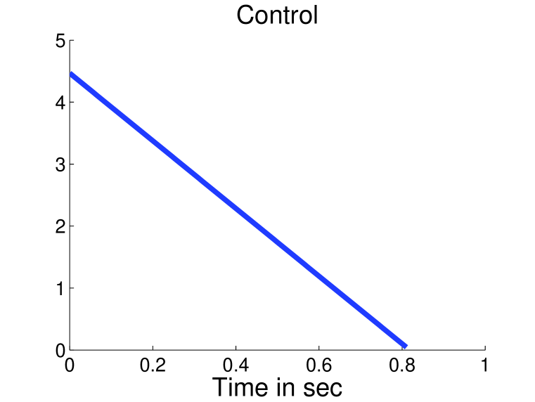
(a) R=0.1

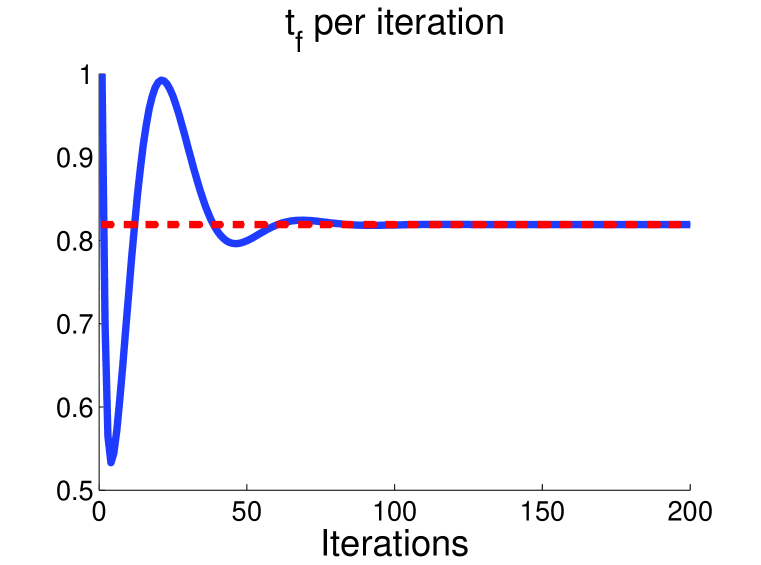
(b) R=0.1

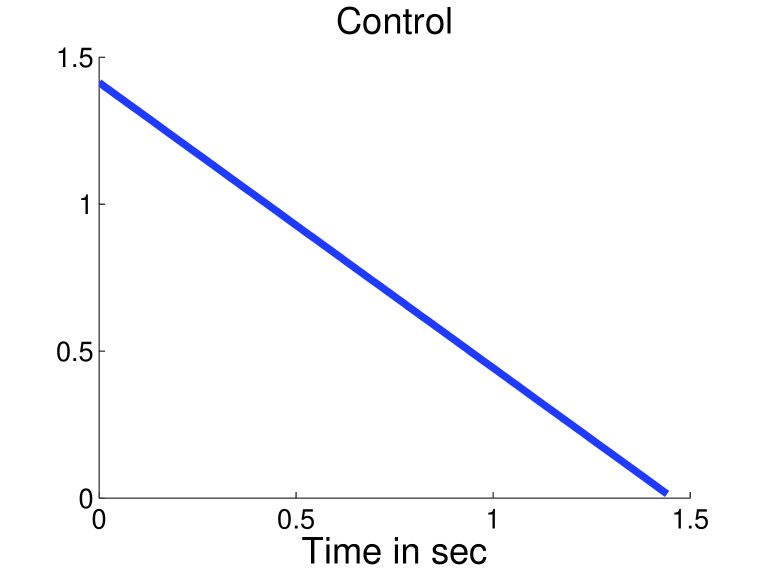
(c) R=1

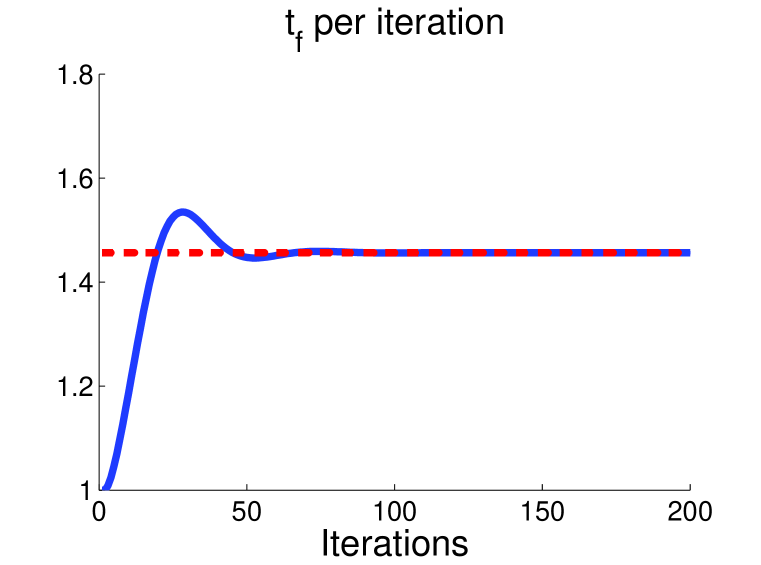
(d) R=1

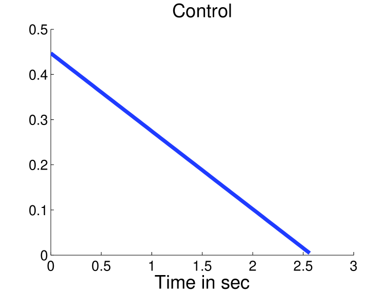
(e) R=10

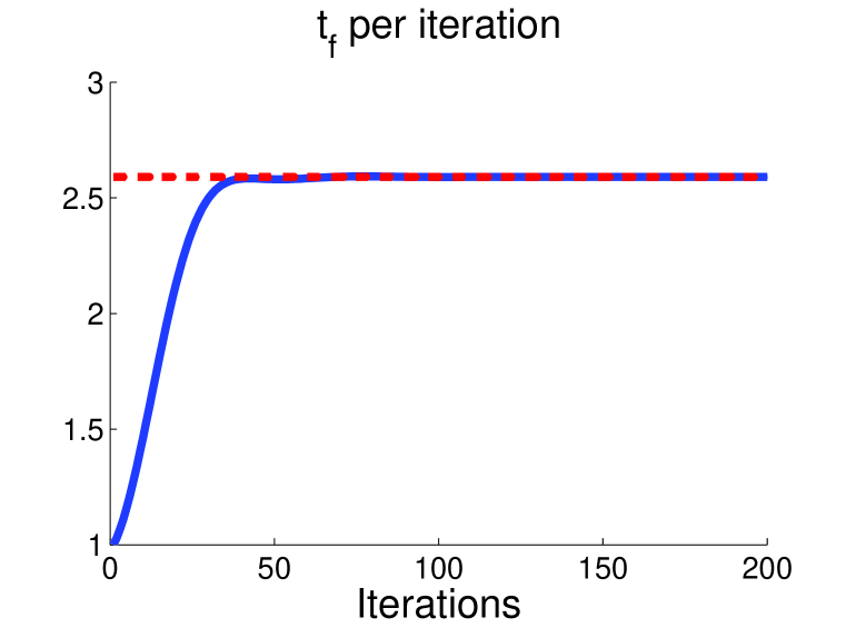
(f) R=10

Figure 1: Figure 1(a), 1(c), 1(e) show the numerical optimal control for the cases when $R=0.1,1,10$, respectively. Figure 1(b), 1(d), 1(f) present the $t_{f}$ per iteration for the cases when $R=0.1,1,10$, respectively. Dashed red lines represents the according analytical optimal $t_{f}$.

3.2 Cart Pole

In this subsection, we apply our algorithm on the inverted pendulum on a cart, as known as the cart pole problem, with $M=10$ the mass of the cart, $m=1$ and $l=0.5$ are the mass and length of the pendulum, $g=9.8$ the gravitational acceleration and $u$ the force applied to the cart. The state ${\bf x}=[x,\dot{x},\theta,\dot{\theta}]$. The goal is to bring the state from ${\bf x}(0)=[0,0,\pi,0]$ to $p=[0,0,0,0]$, which represents the case where the pendulum is pointing strait up. The cost function is given by

$$J=\frac{1}{2}\int_{0}^{t_{f}}[c_{t}+({\bf x}-p)^{{}^{\mathsf{T}}}Q({\bf x}-p)+{\bf u}^{{}^{\mathsf{T}}}R_{{\bf u}}{\bf u}]+\lambda^{{}^{\mathsf{T}}}([{\bf x}_{3}(t_{f});{\bf x}_{4}(t_{f})]-[p_{3};p_{4}]),$$

where $Q=\text{diag}\{0,0,1,1\}$ and $R_{{\bf u}}=0.01$. Initial values are given as $t_{f}=1$, $\lambda=[0,0]^{{}^{\mathsf{T}}}$. The multipliers $\gamma=0.05$ and $\epsilon=0.05$. We run the algorithm for 300 iterations and the convergence is achieved at around 200th iteration. Figure 3(a) presents the optimal control ${\bf u}^{*}$. The corresponding optimal trajectories of the states are depicted in Figure 2. Cost and $t_{f}$ per iteration are shown in Figure 3(b) and 3(c), respectively.

Figure 2: Optimal trajectories of the states in blue. Red lines represent the desired terminal states.

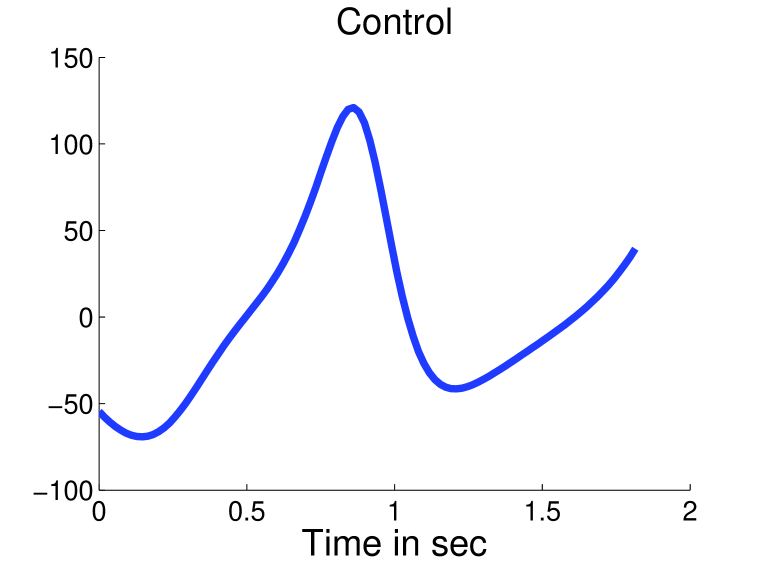
(a) Optimal control of the cart pole system.

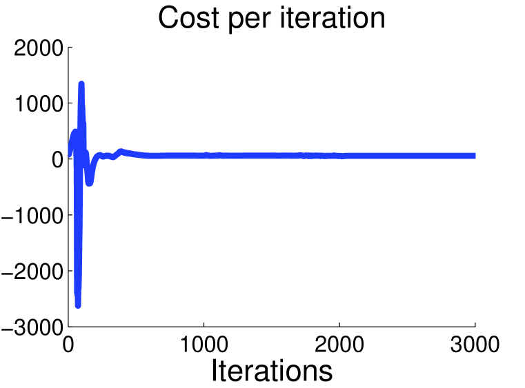
(b) Cost per iteration.

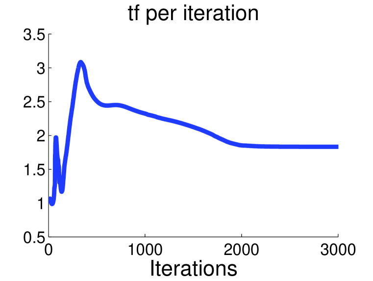
(c) $t_{f}$ per iteration.

Figure 3: Cost and $t_{f}$ per iteration for the cart pole system.

3.3 Quadrotor

The dynamic model of the quadrotor includes 16 states: 3 for the position (${\bf r}=(x,y,z)^{{}^{\mathsf{T}}}$), 3 for the Euler angles ($\Phi=(\phi,\theta,\psi)^{{}^{\mathsf{T}}}$), 3 for the velocity ($\dot{{\bf r}}=(\dot{x},\dot{y},\dot{z})^{{}^{\mathsf{T}}}$), 3 for the body angular rates ($\dot{\Phi}=(p,q,r)^{{}^{\mathsf{T}}}$) and 4 for the motor speeds ($\Omega=(\omega_{1},\omega_{2},\omega_{3},\omega_{4})^{{}^{\mathsf{T}}}$). The corresponding dynamics of the quadrotor is given as follows:

$$\frac{\textrm{d}{\bf x}}{\textrm{d}t}=f({\bf x})+G{\bf u},$$ (29)

where ${\bf x}=[{\bf r},\Phi,\dot{{\bf r}},\dot{\Phi},\Omega]^{{}^{\mathsf{T}}}\in\mathbb{R}^{16}$, and ${\bf u}=(u_{1},u_{2},u_{3},u_{4})^{{}^{\mathsf{T}}}\in\mathbb{R}^{4}$ is the control vector, where $u_{1}$ represents the thrust force, and $u_{2},u_{3},u_{4}$ represent the pitching, rolling, yawing moments, respectively. The corresponding cost function is defined as $J=\frac{1}{2}\int_{0}^{t_{f}}[c_{t}+({\bf x}-p)^{{}^{\mathsf{T}}}Q({\bf x}-p)+{\bf u}^{{}^{\mathsf{T}}}R_{{\bf u}}{\bf u}]+\frac{1}{2}({\bf x}(t_{f})-p)^{{}^{\mathsf{T}}}Q_{f}({\bf x}(t_{f})-p)+\lambda^{{}^{\mathsf{T}}}([{\bf x}_{1}(t_{f});\dots;{\bf x}_{6}(t_{f})]-[p_{1};\dots;p_{6}]),$ where $p=[p_{1};\dots;p_{16}]\in\mathbb{R}^{16}$ denotes the desired terminal states. In the simulation, we set

$$p(i)=\begin{cases}1,i=3;\\ 0,\text{otherwise},\end{cases}\quad\text{and}\quad Q_{f}(i,i)=\begin{cases}10^{7},i=1,2,3;\\ 10^{6},i=4,\dots,9;\\ 10^{5},i=10,11,12;\\ 0,\text{otherwise},\end{cases}$$ (30)

and all the off-diagonal terms are assigned to $0$. $Q=0.01Q_{f}.$ $R_{{\bf u}}=0.0001I$. $\gamma=0.02$ and $\epsilon=0.02$. The desired terminal state $p$ is chosen for the quadrotor to execute the take-off maneuver. $50$ iterations are included to ensure the convergence and the cost per iteration is presented in Figure 5(b). The corresponding optimal state trajectories are shown in Figure 4. Optimal control ${\bf u}$ is illustrated in Figure 5(a). $t_{f}$ per iteration is presented in Figure 5(c).

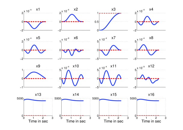
Figure 4: Optimal trajectories of the states of the quadrotor in blue. Dashed red lines represent the desired terminal states.

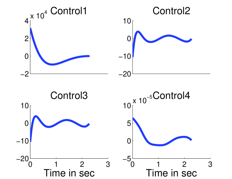
(a) Optimal controls.

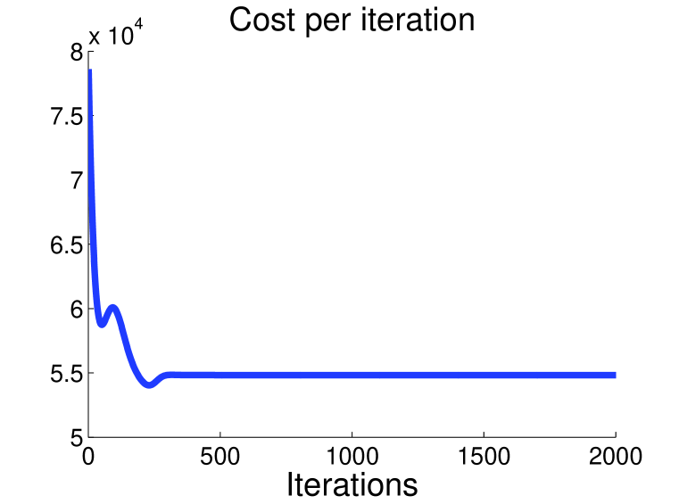
(b) Cost per iteration.

(c) $t_{f}$ per iteration.

Figure 5: Cost and $t_{f}$ per iteration for the quadrotor.

Acknowledgments

References

- [1] D.H. Jacobson and D.Q Mayne. Differential dynamic programming. Elsevier Sci. Publ., 1970.
- [2] Sergey Levine and Pieter Abbeel. Learning neural network policies with guided policy search under unknown dynamics. In Z. Ghahramani, M. Welling, C. Cortes, N.D. Lawrence, and K.Q. Weinberger, editors, Advances in Neural Information Processing Systems 27, pages 1071–1079. Curran Associates, Inc., 2014.
- [3] Y. Pan and E. Theodorou. Probabilistic differential dynamic programming. In Advances in Neural Information Processing Systems (NIPS), pages 1907–1915, 2014.
- [4] J. Morimoto, G. Zeglin, and C. G Atkeson. Minimax differential dynamic programming: Application to a biped walking robot. In Proceedings of 2003 IEEE/RSJ International Conference on Intelligent Robots and Systems (IROS 2003)., volume 2, pages 1927–1932. IEEE, 2003.
- [5] Y. Tassa, N. Mansard, and E. Todorov. Control-limited differential dynamic programming. In 2014 IEEE International Conference on Robotics and Automation (ICRA),, pages 1168–1175. IEEE, 2014.
- [6] Y. Tassa, T. Erez, and W. D. Smart. Receding horizon differential dynamic programming. In NIPS, 2007.
- [7] P. Abbeel, A. Coates, M. Quigley, and A. Y Ng. An application of reinforcement learning to aerobatic helicopter flight. Advances in Neural Information Processing Systems (NIPS), 19:1, 2007.
- [8] E. Todorov and W. Li. A generalized iterative lqg method for locally-optimal feedback control of constrained nonlinear stochastic systems. In American Control Conference, 2005, pages 300–306. IEEE, 2005.
- [9] E. Theodorou, Y. Tassa, and E. Todorov. Stochastic differential dynamic programming. In American Control Conference (ACC), 2010, pages 1125–1132. IEEE, 2010.