Thermal transport in disordered one-dimensional spin chains

Abstract

We study one-dimensional anisotropic XY-Heisenberg spin-$\frac{1}{2}$ chain with weak random fields $h_{i}^{z}S^{z}_{i}$ by means of Jordan-Wigner transformation to spinless Luttinger liquid with disorder and bosonization technique. First we investigate phase diagram of the system in terms of dimensionless disorder $\gamma=\left<h^{2}\right>/J^{2}\ll 1$ and anisotropy parameter $\Delta=J_{z}/J_{xy}$ and find the range of these parameters where disorder is irrelevant in the infrared limit and spin-spin correlations are described by power laws. Then we use the diagram technique in terms of plasmon excitations to study low-temperature behavior of heat conductivity $\kappa$ and spin conductivity $\sigma$ in this power-law phase. The obtained Lorentz number $L\equiv\kappa/\sigma T$ differs from the value derived earlier by means of memory function method. We argue also that in the studied region inelastic scattering is strong enough to suppress quantum interference in the low-temperature limit.

I Introduction

One-dimensional disordered spin chain is an excellent example of strongly correlated quantum system that is well suited to study basic properties of such systems. In particular, studies of disordered spin chains become one of the major playgrounds in the field of Many Body Localization (MBL)  BAA ; Mirlin05 ; HuseReview ; mblpalhuse ; Serbyn1 ; Serbyn2 ; Berkovits14 ; BarLev14 . From the experimental viewpoint, quasi-one-dimensional antiferromagnets exp1 ; exp2 ; exp3 attract considerable attention due to very high thermal conductance, that is believed to be related with integrability of the clean Heisenberg spin-$\frac{1}{2}$ chain Moore1 ; Moore2 . It is known since seminal paperrggiamarchishulz that in 1D competition between interaction and disorder may lead to delocalization and formation of a ground state that is nearly-free from the effects of disorder, see also giamarchibook ; bosons2012 . Numerical studies 1dchainNumerical confirm that qualitative conclusion. In order to provide delocalization, interaction should be sufficiently strong and attractive, so this problem bears some resemblance with a model of superconductor-insulator transition in higher-dimensional systems FIM10 . Looking from that perspective, it seems useful to develop a quantitative theory of the delocalized phase of one-dimensional quantum system with a bare disorder that is ”screened” by interactions. In particular, it is important to study heat transport in such a system, that is expected to be dominated by the remains of the disorder potential.

Here we will study the properties of anisotropic XXZ spin chain in a random transverse magnetic field, which is described by the Hamiltonian (we assume $J>0$):

$$\hat{H}=-J\sum_{n}\left(\hat{S}_{n}^{x}\hat{S}_{n+1}^{x}+\hat{S}_{n}^{y}\hat{S}_{n+1}^{y}+\Delta\hat{S}_{n}^{z}\hat{S}_{n+1}^{z}+\frac{h_{n}}{J}\hat{S}_{n}^{z}\right)$$ (1)

By means of the Jordan-Wigner (JW) transformation the Hamiltonian (1) can be reduced to the Hamiltonian of interacting spinless fermions (here $\rho_{n}=c_{n}^{\dagger}c_{n}-\frac{1}{2}$):

$$\hat{H}=-J\sum_{n}\left(\frac{1}{2}c_{n}^{\dagger}c_{n+1}+h.c+\Delta\rho_{n}\rho_{n+1}+\frac{h_{n}}{J}\rho_{n}\right)$$ (2)

The anisotropy parameter $\Delta$ can be both positive and negative, which corresponds to the effective attraction or repulsion between JW fermions, respectively.

We will consider random fields to be relatively small so that $\gamma=\left<h^{2}\right>/J^{2}\ll 1$, and with zero average $\left<h\right>=0$. Thus our system is, on average, symmetric with respect to $z\mapsto-z$ reflection, which translates into the particle-hole symmetry in terms of JW fermions. It ensures that in the quasiparticle spectrum $\varepsilon(k)$ only odd powers of $k$ survive.

The goal of this paper is to study low-temperature transport properties, spin and heat conductivity, in the range of parameters $\left(\Delta,\gamma\right)$ where $T=0$ spin-spin correlations decay as a power law with a distance. The rest of the paper is organized as follows: in Sec.II we study the phase diagram by means of Renormalization Group approach formulated in rggiamarchishulz . Sec.III is devoted to formulation and application of the Keldysh approach to the transport properties of disordered Luttinger liquid model that is an appropriate low-energy approximation for the lattice fermion model (2); in Sec.III A, spin and heat conductivities ($\sigma$ and $\kappa$) are studied within the region $\frac{1}{2}\leq\Delta\leq 1$ where disorder is irrelevant in the RG sense; next, in Sec.III B we discuss specific behavior of $\sigma$ and $\kappa$ near the critical point $\Delta=\frac{1}{2}$; the role of quantum interference corrections and decoherence is discussed in Sec. III C, and the role of spectrum nonlinearity is considered in Sec.III D. Finally, we present our Conclusions in Sec. IV.

II Luttinger liquid description and phase diagram

In the clean limit $h_{n}=0$ and in the region $-1<\Delta<1$ excitation spectrum of the interacting one-dimensional fermion system (2) is gapless; then low-energy and long-distance properties of the system are known to be described by the Luttinger liquid (LL) model giamarchibook . It allows to rewrite the Hamiltonian in terms of fermion density excitations — plasmons. LL model is formulated in terms of canonically conjugated plasmon fields $\left[\phi(x),\Pi(y)\right]=i\delta(x-y)$; in the linear approximation for the quasiparticle spectrum, the Hamiltonian of the LL model reads

$$\hat{H}_{LL}=\frac{1}{2\pi}\int dx\left(\frac{u}{K}(\partial_{x}\phi)^{2}+uK(\pi\Pi)^{2}\right).$$ (3)

Here $u$ is plasmon velocity and $K$ is dimensionless Luttinger parameter; these parameters are determined, via the Bethe Ansatz solution for XXZ model, by the values of $J$ and $\Delta$, see (giamarchibook, , p.167):

$$\Delta=\cos\frac{\pi}{2K},\quad u=\frac{Ja}{2}\frac{\sin(\pi/2K)}{1-1/2K}$$ (4)

where $a$ is the lattice constant.

In our model (2) disorder couples to the fermion density $\rho_{n}$; in the LL continuum limit it reads as $\rho(x)=-\frac{1}{\pi}\partial_{x}\phi+\frac{1}{\pi a}\cos(2k_{F}x-2\phi)$. First and second terms in the above expression correspond to the slow ($q\sim 0$) and fast oscillating ($q\sim 2k_{F}$) parts. Thus there are two types of scattering of one-dimensional fermions by disorder: forward and backward. Forward scattering is irrelevant within the linear approximation for the spectrum, since the corresponding term in the LL Hamiltonian can be eliminated completely by the redefinition of phase $\phi(x)$. Backward fermion scattering with momentum transfer $q\sim 2k_{F}$ is the only effect one should take into account then. Thus we need only $q\sim 2k_{F}$ part of original random potential, this part is described by the random Gaussian complex field $\xi(x)$ with $\left<\xi(x)\xi^{*}(y)\right>=D\delta(x-y)$ and $D=\left<h^{2}\right>a$. Disorder contribution to the Hamiltonian reads as follows:

$$\hat{H}_{dis}=-\frac{1}{2\pi\alpha}\int dx(\xi(x)e^{-2i\phi}+\xi^{*}(x)e^{2i\phi})$$ (5)

Renormalization Group approach to disordered Luttinger liquid was formulated in rggiamarchishulz . It is convenient to introduce dimensionless disorder parameter

$$g=\frac{2Da}{\pi u^{2}}=\frac{8(1-1/2K)^{2}}{\pi\sin^{2}(\pi/2K)}\gamma$$ (6)

In terms of this parameter and logarithmic scaling parameter $\xi=\ln\frac{\widetilde{a}}{a}$ (with $\widetilde{a}$ being running ultraviolet cutoff), RG equations reads as follows:

$$\begin{cases}\frac{du}{d\xi}&=-\frac{uK}{2}g\\ \frac{dK}{d\xi}&=-\frac{K^{2}}{2}g\\ \frac{dg}{d\xi}&=(3-2K)g.\end{cases}$$ (7)

These equations can be solved analytically exploiting its first integral $I(K,g)=\frac{9}{8}(\frac{6}{K}+4\ln K-g)$. This solution yields phase diagram shown in Fig. 1. ”Delocalized” region lies, in the limit of very weak disorder, in the range $\frac{1}{2}<\Delta<1$. Upon increase of $\gamma$, delocalized region shrinks and eventually disappears already at $\gamma\approx 0.1$. Everywhere in the delocalized phase effective disorder $g(\xi)$ decreases with $\xi$. Actually the derivation of the RG equations (7) as it was performed in rggiamarchishulz is valid quantitatively in the vicinity of the point $K=3/2$ only, where disorder-induced corrections to the parameter $K$ are logarithmic; for large $K$ these equations can be used for qualitative analysis only. Note that the drop of the critical disorder $\gamma$ near the point $\Delta=1$ is trivially related to the decrease of the effective Luttinger velocity $u$, see Eqs.(4).

Phase diagram obtained by the analysis of RG equations can be compared with the numeric phase diagram from Ref.1dchainNumerical (its boundary is shown by the dashed line in Fig. 1). According to these numerical data, the delocalized region covers much smaller part of the phase diagram than the RG calculations predict. We expect that the major source of this discrepancy is due to inapplicability of the RG equations (7) at large $K$ values. Another reason could be related with the effects of spectrum nonlinearity that becomes important close to $\Delta=1$. On the other hand, near the point $K=3/2$ numerical data 1dchainNumerical suggest delocalization at the values of $\gamma$ which are above our critical line; we believe that this discrepancy comes from limited accuracy of the numerical data, due to finite size effects which becomes most prominent at very weak disorder.

’

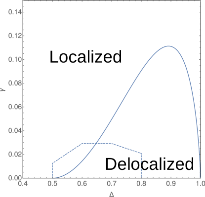
Figure 1: Approximate phase diagram found from the RG calculations for the Luttinger liquid model with linear spectrum. Dashed line corresponds to phase boundary obtained in Ref. 1dchainNumerical .

Equal-time spin-spin correlation function $\langle S^{+}(0)S^{-}(x)\rangle$ decays as a power law at $\Delta>\frac{1}{2}$, as one can read of Ref. bosons2012 where two-loop RG calculation was performed. At smaller $\Delta<\frac{1}{2}$ renormalized disorder parameter $g(\xi)$ grows with $\xi$, and one expects exponential decay of $\langle S^{+}(0)S^{-}(x)\rangle$ at $x\geq L_{c}$, where correlation length $L_{c}\propto\gamma^{1/(2K-3)}$, see rggiamarchishulz .

Note that for the case of XY model with random transverse fields (i.e. $\Delta=0$) exponential decay of $\langle S^{+}(0)S^{-}(x)\rangle$ follows directly from single-particle localization in 1D, as proven rigorously in Ref. Klein . However, at general $\Delta<\frac{1}{2}$ the relation between growth of effective disorder upon RG and Anderson localization is far from being obvious, since the RG calculation  rggiamarchishulz does not contain any multiple-impurity interference effects, see mirlintransport ; mirlincdw .

Below we will focus on delocalized phase $\frac{1}{2}<\Delta<1$, that corresponds to the range of $\frac{3}{2}<K<\infty$, where renormalized disorder constant $g$ is small, and one can obtain transport properties using perturbation theory for bosonic LL model with renormalized parameters.

III Transport properties

Here we proceed from the Hamiltonian description defined by Eqs.(3,5) to the Keldysh action for the LL model with disorder. Total Keldysh action $S_{tot}$ consists of trivial free boson part $S_{0}$ and disorder-related part coming directly from Eq.(5):

$$S_{dis}=\frac{1}{2\pi\alpha}\int_{C}dtdx(\xi(x)e^{-2i\phi}+\xi^{*}(x)e^{2i\phi})$$ (8)

We integrate $\exp(iS_{tot})$ over random Gaussian field $\xi(x)$ and perform Keldysh rotation introducing classical $\phi_{cl}=\frac{1}{2}(\phi_{+}+\phi_{-})$ and quantum $\phi_{q}=\phi_{+}-\phi_{-}$ fields components, arriving finally at the effective disorder action

$$S_{dis}=\frac{iD}{\pi^{2}a^{2}}\int dt_{1}dt_{2}dx\cos 2(\phi_{1cl}-\phi_{2cl})\sin\phi_{1q}\sin\phi_{2q}$$ (9)

In order to obtain self-energy for retarded Green function in the lowest order over $S_{dis}$ we consider first order correction to it, which reads

$$i\delta G_{R}^{(1)}(\mathbf{y}-\mathbf{y}^{\prime})=\frac{iD}{\pi^{2}\alpha^{2}}\intop dt_{1}dt_{2}\int dx_{12}\times$$

$$\times\left\langle\phi_{cl}\phi_{q}^{\prime}\cos(2(\phi_{1cl}-\phi_{2cl}))\sin\phi_{1q}\sin\phi_{2q}\right\rangle_{0}$$ (10)

Here we used notation $\mathbf{y}=(y,t)$ and $\phi_{i}=\phi(y,t_{i})$. Performing Wick’s contraction, one finds two diagrams (see Fig. 2), from which we extract retarded bosonic self-energy $\Sigma_{R}(\omega)$; the corresponding analytical expression reads

$$\Sigma_{R}(\omega)=-\frac{4D}{\pi^{2}a^{2}}\int_{0}^{\infty}dt(1-e^{i\omega t})\times$$

$$\times e^{2i(G_{K}(t)-G_{K}(0))}\sin 2G_{R}(t)$$ (11)

where bare retarded and Keldysh components of the Green function are as follows

$$G_{R}^{(0)}(\omega,q)=\frac{\pi uK}{(\omega+i0)^{2}-u^{2}q^{2}}$$ (12)

$$G_{R}^{(0)}(t,x)=-\frac{\pi K}{2}\theta(t)\theta(ut-|x|)$$ (13)

$$G_{K}^{(0)}(\omega)=\coth\frac{\beta\omega}{2}(G_{R}^{(0)}(\omega)-G_{A}^{(0)}(\omega))$$ (14)

Inverse Fourier transformation of the Keldysh component $G_{K}^{(0)}(\omega)$ to the real space-time, $G_{K}^{(0)}(t,x)$, is infrared-divergent; it is sufficient to use the difference $G_{K}^{(0)}(t,x)-G_{K}^{(0)}(0,0)$ which is finite:

$$G_{K}^{(0)}(t,x)-G_{K}^{(0)}(0,0)=$$

$$=i\frac{K}{2}\ln\left(\frac{u^{2}\beta^{2}}{\pi^{2}\alpha^{2}}\left|\sinh\frac{\pi(x+ut)}{u\beta}\sinh\frac{\pi(x-ut)}{u\beta}\right|\right)$$ (15)

At low temperatures $T\ll J$ two different types of contributions to the disorder-induced self-energy can be separated: virtual transitions with $T\ll\omega\leq J$ and real (dissipative) transitions with $\omega\leq T$. First contribution lead to logarithmic renormalization of the model parameters yielding RG equations (7) described above; second contribution yields dissipative behavior of corresponding self-energy $\Sigma_{R}=-i\omega/u\pi K\tau$. Direct calculation yields the following expression for momentum relaxation rate:

$$\frac{1}{\tau(T)}=\frac{2DK}{u}\frac{\Gamma^{2}(K)}{\Gamma(2K)}\left(\frac{2\pi aT}{u}\right)^{2K-2}$$ (16)

According to Eq.(16), product $T\tau\propto T^{3-2K}$ diverges as $T\to 0$ in the delocalized phase. Full Green function then reads as follows:

$$G_{R}(q,\omega)=\frac{\pi uK}{\omega^{2}-u^{2}q^{2}+i\omega/\tau}.$$ (17)

(a)

(b)

Figure 2: Lowest order diagrams for the retarded self energy $\Sigma_{R}(\omega)$. Dashed lines correspond to disorder average $\left<\xi(x)\xi^{*}(y)\right>$ and wavy lines correspond to averaging of cosine or sine of boson fields

III.1 Spin and heat conductivities

To obtain transport properties, one can apply Kubo formulas. Expressions for spin and energy currents can be derived from corresponding continuity equation $\partial_{t}\rho_{\alpha}+\nabla j_{\alpha}=0$ (index $\alpha$ corresponds to either spin or energy), and using classical equations of motion. For the Hamiltonian of the form $\hat{H}=\int dx\rho_{E}(\phi(x),\nabla\phi(x),\Pi(x))$, equations of motion reads as follows:

$$\partial_{t}\phi=\frac{\partial\rho_{E}}{\partial\Pi},\quad\partial_{t}\Pi=-\frac{\partial\rho_{E}}{\partial\phi}+\nabla\frac{\partial\rho_{E}}{\partial(\nabla\phi)}$$ (18)

so energy density obeys the following continuity equation:

$$\partial_{t}\rho_{E}=\frac{\partial\rho_{E}}{\partial\phi}\partial_{t}\phi+\frac{\partial\rho_{E}}{\partial\nabla\phi}\partial_{t}\nabla\phi+\frac{\partial\rho_{E}}{\partial\Pi}\partial_{t}\Pi=\nabla\left(\frac{\partial\rho_{E}}{\partial\nabla\phi}\frac{\partial\rho_{E}}{\partial\Pi}\right)$$ (19)

and similarly for spin density. Considering total Hamiltonian consisting of two contributions (3) and (5), we arrive at the following expressions for currents:

$$j_{s}=\frac{1}{\pi}\partial_{t}\phi,\qquad j_{E}=-\frac{u}{\pi K}\partial_{t}\phi\nabla\phi.$$ (20)

We emphasize that Eqs.(20) provide exact (within Luttinger liquid approximation) expressions for both spin and thermal currents. Surprisingly, in the LL approximation the energy current does not contain any terms related to the presence of backscattering. In Appendix A we provide a detailed derivation of the energy current, starting from the lattice fermion model (1), and show that backscattering does produce additional terms for the energy current, but these terms vanish in the continuous LL limit, when $a\to 0$ at some fixed value of the product $Ja$.

Spin transport is governed by the single-plasmon Green function, while for energy transport we need to calculate correlation function of four $\phi$ fields. Applying Kubo formula for spin conductivity, we reproduce Drude-like result of Refs.mirlincdw ; orignac .

$$\sigma(\omega)=\frac{i\omega}{\pi^{2}}G_{R}(\omega,q=0)=\frac{uK}{\pi}\frac{\tau}{1-i\omega\tau}$$ (21)

valid at $\omega\ll T$.

Thermal conductivity $\kappa$ is expressed in terms of so-called “thermal susceptibility” $\chi_{E}(q,\omega)$ as $\kappa(\omega)=-\frac{i\beta}{\omega+i0}(\chi_{E}(0,\omega)-\chi_{E}(0,0))$. Introducing short notation $\textbf{x}=(x,t)$, and $\textbf{q}=(q,\omega)$, expression for thermal susceptibility in real space reads as follows:

$$\chi_{E}(\textbf{x}_{1}-\textbf{x}_{2})=i\frac{u^{2}}{\pi^{2}K^{2}}\left\langle(\partial_{t}\phi_{1}\nabla\phi_{1})_{cl}(\partial_{t}\phi_{2}\nabla\phi_{2})_{q}\right\rangle$$ (22)

and $\chi(\textbf{q})$ is the Fourier transform of this expression.

Figure 3: Loop diagram for “thermal susceptibility” $\chi_{E}$. Thermal current vertices act as the following combinations of derivatives: $(\partial_{t}\nabla^{\prime}+\partial^{\prime}_{t}\nabla)$, with derivatives $\partial_{t}$, $\nabla$ acting on one $\phi$ field in the vertex and $\partial_{t}^{\prime}$, $\nabla^{\prime}$ acting on another one.

In the dc limit $\omega\to 0$ one finds $\kappa=-i\beta\left.\frac{\partial\chi_{E}}{\partial\omega}\right|_{\omega=0}$. Applying Wick’s theorem, one finds:

$$\chi_{E}(\mathbf{q}^{\prime}) =-i\frac{u^{2}}{2\pi^{2}K^{2}}\int(d^{2}\mathbf{q})\left[2\omega q-\frac{\omega^{\prime}q^{\prime}}{2}\right]^{2}\times$$ (23)

$$\times G_{K}(\mathbf{q}+\frac{\mathbf{q}^{\prime}}{2})G_{A}(\mathbf{q}-\frac{\mathbf{q}^{\prime}}{2})$$

Calculating it in the $\omega\to 0$ limit with “dressed” Green functions, we arrive at:

$$\kappa=\frac{1}{4}u\beta^{2}\tau\int\frac{d\omega}{2\pi}\frac{\omega^{2}}{\sinh^{2}\frac{\beta\omega}{2}}=\frac{\pi}{3}uT\tau$$ (24)

Comparison between Eqs.(21,24) provides us with the value of the Lorentz number

$$L=\frac{\kappa}{\sigma T}=\frac{\pi^{2}}{3K}$$ (25)

which matches its standard Fermi liquid value $L_{FL}=\frac{\pi^{2}}{3}$ for $K=1$. Note that our result (25) differs from one obtained in orignac by means of memory function formalism. We believe that this discrepancy is due to limitations of the memory function formalism  orignac which is based on extrapolation from the large-$\omega$ region to the static limit. Indeed, frequency-dependent thermal conductance $\kappa(\omega)$ depends on two different frequency scales, $T$ and $1/\tau$; according to Eq.(16), in the region $K>3/2$ one always has $T\gg 1/\tau(T)$ in the low-temperature limit. In order to obtain static thermal conductivity, one should be able to compute $\kappa(\omega)$ at $\omega\tau\ll 1$, whereas memory function method is based upon the calculation of the high-frequency limit $\kappa(\omega\geq 1/T)$ and further extrapolation to zero frequency. We believe that the presence of two parametrically different frequency scales $1/\tau$ and $T$ makes such an extrapolation unreliable.

The above calculation leading to Eqs.(24) and (25) should be performed, in general, with the parameters $(g,K)$ renormalized (due to RG equations (7)) down to the temperature scale $\xi_{T}$. If bare parameters $(g,K)$ are in the bulk of delocalized phase (not too close to the transition line) one can neglect renormalization of $K$ and $u$ due to disorder, leading to the results for spin and thermal conductivities which depend on the scale $\xi_{T}$ via scattering time $\tau$ only, see (16). Then the result is given by Eqs. (21), (24) with bare parameters.

Near the transition line one should take renormalization of all the parameters simultaneously. Below we will see how it affects physical properties of the system.

III.2 Vicinity of the point $\Delta=\frac{1}{2}$

Expanding first integral of system (7) by $K-\frac{3}{2}$, or, equivalently, $\Delta-\frac{1}{2}$, one obtains:

$$I-I_{c}=\frac{27}{\pi^{2}}\left(\Delta-\frac{1}{2}\right)^{2}-\frac{16}{3\pi}\gamma$$ (26)

The equality $I=I_{c}$ yields the phase boundary of the delocalized state in the form $\left(\Delta-\frac{1}{2}\right)^{2}=\frac{16\pi}{81}\gamma$.

Solution of the equations (7) can be expressed in terms of vicinity to transition line $\alpha=\sqrt{I-I_{c}}\ll 1$:

$$\begin{cases}u(\xi)&=u\exp\left(\frac{2}{3}K(\xi)-1\right)\\ K(\xi)&=\alpha\coth\alpha(\xi+\xi_{0})\\ g(\xi)&=\frac{8\alpha^{2}}{9\sinh^{2}\alpha(\xi+\xi_{0})}\end{cases}$$ (27)

where $\xi_{0}$ depends on initial values of parameters. Considering temperature to be low enough (so $\xi_{T}\gg|\xi_{0}|,1/\alpha$), one obtains low-temperature behavior of renormalized parameters $g(\xi_{T})\simeq\alpha^{2}\exp(-2\alpha\xi)\simeq\alpha^{2}(T/J)^{2\alpha}$ and $K(\xi_{T})-\frac{3}{2}\simeq\alpha=\mathrm{const}$.

Now we repeat the above calculations leading to nonzero $\mathrm{Im}\Sigma(\omega)$ and obtain Drude-type formulae with corrected power-law exponent $\alpha$:

$$\sigma\simeq\alpha^{-2}a(T/J)^{-1-2\alpha}\,\qquad\kappa\simeq J\alpha^{-2}a(T/J)^{-2\alpha}$$ (28)

The Lorentz number is still given by Eq.(25) once renormalization $K\to K(\xi_{T})$ is taken into account. Modifications of $K$ and $\alpha$ are negligible if $g\ll(K-\frac{3}{2})^{2}$.

III.3 Smallness of the interference corrections.

Our result for the heat conductance, Eq. (24), was obtained within Drude-type approximation. Since our system is one-dimensional, some care should be exercised to check if the effects of quantum interference and Anderson localization could affect that result. To begin with, it is useful to employ the result of Ref.mirlintransport where the same issue was considered for disordered Luttinger liquid with a weak interaction, $|K-1|\ll 1$. Namely, it was found in mirlintransport that interference corrections are negligible at sufficiently high temperatures $T\geq\tau^{-1}(T)(K-1)^{-2}$. We are working at $K>3/2$ and the corresponding condition is just $T\gg 1/\tau(T)$ which is always fulfilled at low temperatures according to Eq.(16).

To estimate interference corrections more accurately, we examine expression for “thermal susceptibility” to higher order in $S_{dis}$ adding impurity lines connecting upper and lower Green functions drown in Fig.3. First order correction (with single impurity line) vanishes at zero external momentum due to gradient structure of energy current vertex. First non-trivial corrections are due to diagrams shown in Fig. 4; the corresponding analytical expressions yield:

$$\delta\chi_{E}(\mathbf{x}-\mathbf{x}^{\prime})=\frac{1}{2}\left(\frac{iD}{\pi^{2}\alpha^{2}}\right)^{2}\int dt_{1}dt_{2}dt_{3}dt_{4}\times$$

$$\times\int dx_{12}dx_{34}\Bigg{\langle}\partial_{t}\phi_{cl}(\mathbf{x})\nabla\phi_{cl}(\mathbf{x})\times$$

$$\times\left(\partial_{t}\phi_{cl}(\mathbf{x}^{\prime})\nabla\phi_{q}(\mathbf{x}^{\prime})+\partial_{t}\phi_{q}(\mathbf{x}^{\prime})\nabla\phi_{cl}(\mathbf{x}^{\prime})\right)\times$$

$$\times\cos(2\phi_{1cl}-2\phi_{2cl})\sin\phi_{1q}\sin\phi_{2q}\times$$

$$\times\cos(2\phi_{3cl}-2\phi_{4cl})\sin\phi_{3q}\sin\phi_{4q}\Bigg{\rangle}$$ (29)

Grayed box correspond to sine and cosine average and consists of infinite number of boson propagators connecting all the points. Generally speaking, such box depends on all the ingoing energies and momentums. However, direct calculation shows that it contains factors $e^{2i(G_{K}(t_{i}-t_{j})-G_{K}(0))}\propto 1/\sinh^{2K}\pi T(t_{i}-t_{j})$, which impose effective constraint for time differences: any such diagram is very small unless the condition $|t_{i}-t_{j}|\leq 1/T$ is fulfilled. On the other hand, typical time scale for the dressed “external” (w.r.t. to the ”grey area”) propagators is $\tau(T)\gg 1/T$; therefore, up to the leading order in $1/T\tau(T)\ll 1$ one can try to shrink all four space-time impurity points in Fig. 4 into single one (see Fig. 5). However, calculation of the remaining integrals result in a zero result, due to vector structure of the current vertex. Therefore, nonzero vertex corrections appear in the next order in $1/T\tau(T)\ll 1$ only, and are small at low $T$ in the whole “delocalized” phase $K>3/2$.

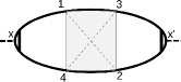
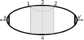
Figure 4: Non-trivial corrections to “thermal susceptibility”. Dashed lines correspond to same impurity, and grayed area correspond to average of cosine and sine of $\phi$ fields. See main text for the analytical expressions.

Figure 5: Effective form of the diagram for the vertex correction to thermal susceptibility, valid in the leading order of expansion over $1/T\tau(T)\ll 1$

III.4 Spectrum nonlinearity effects

At the Heisenberg isotropic point $\Delta=1$ in the clean system the spectrum of excitations is quadratic and system is no longer described by Luttinger liquid model. In the vicinity to this point plasmon velocity vanishes as $u=Ja\sqrt{(1-\Delta)/2}$; since dimensionless disorder strength $g$ depend on velocity $u$ and interaction parameter $K$, see Eq.(6), this narrows the region where perturbation theory in powers of small $g$ is applicable to $\left<h^{2}\right>/J^{2}\ll(1-\Delta)^{3/2}$.

However spectrum nonlinearity effects at finite temperatures might become relevant long before $\Delta=1$ critical point. Let us make some estimates. Due to particle-hole symmetry, only odd powers in quasiparticle spectrum survive; first non-vanishing contribution to dispersion relation will be $\delta\epsilon\sim\frac{u}{a}(ka)^{3}$. At finite temperatures this yield new energy scale $\delta\epsilon\sim T(Ta/u)^{2}$; such energy scale should be compared with scattering ratio $1/\tau\sim ug/a(T/J)^{2K-2}$. Therefore we conclude that spectrum nonlinearity will be important and should be taken into account when $\left(T/J\right)^{5-2K}\geq\left\langle h^{2}\right\rangle/J^{2}$.

For $K<5/2$ it leads to the threshold for the temperature, above which nonlinearity effects are expected to be important, $T_{*}\sim J(\left<h^{2}\right>/J^{2})^{1/(5K-2)}$; on the contrary, at $K>5/2$ nonlinearity is always important at low temperatures. In terms of the $\Delta$ parameter, the borderline at $K=5/2$ corresponds to $\Delta=\cos\pi/5=(1+\sqrt{5})/4\approx 0.81$.

IV Conclusions

We have analyzed spin and thermal conductance of XXZ spin chain with random-field disorder in the parameter region where major source of disorder (backscattering of Jordan-Wigner fermions) is suppressed by quantum fluctuations and irrelevant in the RG sense at low temperatures. Within the standard bosonization scheme the problem is reduced to the Luttinger liquid model with linear spectrum $\varepsilon(k)\simeq uk$ and Luttinger interaction parameter $K$ in the range $3/2<K<\infty$, which corresponds to $1/2<\Delta<1$ in terms of original anisotropy parameter $\Delta=J_{z}/J$ of the spin chain. We derive a phase boundary in terms of $\Delta$ and normalized disorder $\left<h^{2}\right>/J^{2}$ and compare it with the numerical result of Ref. 1dchainNumerical . Then we use diagrammatic Drude-like calculation of thermal and spin conductivities and found Lorentz number, (25), different from the previous result orignac . We also argue that quantum interference (the effects beyond Drude approximation) is irrelevant at low temperatures due to strong enough inelastic scattering at $1/2<\Delta<1$.

These results were obtained neglecting forward scattering of Jordan-Wigner fermions by disorder, which is allowed as long as the approximation of LL model with linear spectrum is employed. However, this approximation is not evidently correct everywhere in the delocalized phase. We estimated region where it might lead to qualitatively different low-temperature behavior as $\Delta>\cos\frac{\pi}{5}$. The effects of spectrum non-linearity will be considered in the separate publication.

We have not studied the region $\Delta<\frac{1}{2}$ where localization due to disorder is expected; here it is very interesting to consider the close vicinity of the transition point, $\frac{1}{2}-\Delta\ll 1$ and $\left<h^{2}\right>/J^{2}\ll 1$ and search for the existence of localization-delocalization threshold as function of excitation energy, like the one studied in FIM10 ; FI15 for the Bethe lattice model.

This research was supported by the Russian Foundation for Basic Research via grant # 13-02-91058 (general phase diagram, Fig.2) and by the Russian Science Foundation via grant # 14-42-00044 (all other results, presented in Eqs.(24,25,28)).

We are grateful to V. E. Kravtsov, K. Michaeli, L. B. Ioffe and K. S. Tikhonov for useful discussions.

Appendix A Derivation of the energy current starting from the lattice model.

For a general Hamiltonian which is a sum of local on-site energy operators $H=\sum_{n}h_{n,n+1}$, with on-site energies which satisfy continuity equation $\partial_{t}h_{n,n+1}+j_{E,n+1}-j_{E,n}=0$ with energy current $j_{E,n}=i\left[h_{n-1,n},h_{n,n+1}\right]$. For particular Hamiltonian (1) on-site energies has the form:

$$h_{n,n+1}=-J\left[\hat{S}_{n}^{x}\hat{S}_{n+1}^{x}+\hat{S}_{n}^{y}S_{n+1}^{y}+\Delta\hat{S}_{n}^{z}\hat{S}_{n+1}^{z}\right]+h_{n}\hat{S}_{n}^{z}$$ (30)

Substituting this expression into the expression for energy current yields two contributions. First contribution is of kinetic nature, it does not contain disorder and can be written in a compact form as a determinant:

$$j_{E,n}^{(kin)}=\mathrm{det}\left(\begin{array}[]{ccc}\hat{S}_{n-1}^{x}&\hat{S}_{n}^{x}&\hat{S}_{n+1}^{x}\\ \hat{S}_{n-1}^{y}&\hat{S}_{n}^{y}&\hat{S}_{n+1}^{y}\\ \Delta\hat{S}_{n-1}^{z}&\hat{S}_{n}^{z}&\Delta\hat{S}_{n+1}^{z}\end{array}\right)$$ (31)

Below we will focus only on the second term, which contains disorder. Corresponding expression in the original spin representation and in the Jordan-Wigner representation reads as follows:

$$j_{E,n}^{(dis)}=-i\frac{J}{2}h_{n}(S_{n-1}^{+}S_{n}^{-}-S_{n-1}^{-}S_{n}^{+})=$$

$$=-i\frac{J}{2}h_{n}(c_{n-1}^{\dagger}c_{n}-c_{n}^{\dagger}c_{n-1})$$ (32)

Next step is to take continuum limit by replacing lattice operators $c_{n}$ with continuous field $\psi(x=na)=c_{n}/\sqrt{a}$ and replacing fields $h_{n}$ with continuous potential $V(x=na)=h_{n}$. Corresponding expression for energy current density then reads as follows:

$$j_{E}^{(dis)}(x)=-i\frac{Ja}{2}V(x)(\psi^{\dagger}(x-a)\psi(x)-\psi^{\dagger}(x)\psi(x-a))$$ (33)

In order to separate forward and backward scattering, we introduce slowly varying in space left- and right-moving fermionic fields $\psi_{L,R}(x)$ with $\psi(x)=e^{ik_{F}x}\psi_{R}(x)+e^{-ik_{F}x}\psi_{L}(x)$. After splitting potential $V(x)$ onto “forward-scattering” part $\eta(x)$ with Fourier harmonics $q\sim 0$ and “backward-scattering” part $\xi(x)$ with $q\sim 2k_{F}$, one obtains contributions to energy current from forward- and backward-scattering processes:

$$j_{E}^{(f.s.)}=\frac{Ja}{2}\eta(x)(\psi_{R}^{\dagger}(x-a)\psi_{R}(x)-\psi_{L}^{\dagger}(x-a)\psi_{L}(x))+$$

$$+h.c.\approx Ja\eta(x)\left(\psi_{R}^{\dagger}(x)\psi_{R}(x)-\psi_{L}^{\dagger}(x)\psi_{L}(x)\right)$$ (34)

$$j_{E}^{(b.s.)}=\frac{Ja}{2}\xi^{*}(\psi_{R}^{\dagger}(x-a)\psi_{L}(x)-\psi_{R}^{\dagger}(x)\psi_{L}(x-a))+$$

$$+h.c.\approx\frac{Ja^{2}}{2}\xi^{*}(-\nabla\psi_{R}^{\dagger}\psi_{L}+\psi_{R}^{\dagger}(x)\nabla\psi_{L})+h.c.$$ (35)

One can see that backward-scattering contribution is of the next order in the small lattice constant $a$ and indeed vanishes in the continuum limit, that is $a\to 0$ keeping $u\propto Ja$ constant.

References

- (1) D.M. Basko, I.L. Aleiner and B.L. Altshuler, Ann. Phys.321, 1126 (2006)
- (2) I.V. Gornyi, A.D. Mirlin and D.G. Polyakov Phys. Rev. Lett. 95, 206603 (2005)
- (3) R. Nandkishore and D.A.Huse, Annual Review of Condensed Matter Physics, 6, 15 (2015).
- (4) A. Pal and D. A.Huse, Phys.Rev.B 82, 174411 (2010)
- (5) M. Serbyn, Z. Papić, and D. A. Abanin Phys. Rev. Lett. 111, 127201 (2013)
- (6) M. Serbyn, Z. Papić, and D. A. Abanin, Phys. Rev. Lett. 110, 260601 (2013).
- (7) R. Berkovits, Phys. Rev. B 89 205137 (2014).
- (8) Y. Bar Lev, G. Cohen, and D.R. Reichman, Phys. Rev. Lett. 114, 100601 (2015).
- (9) A.V. Sologubenko, K. Giannò, H. R. Ott, A. Vietkine, and A. Revcolevschi, Phys.Rev. B 64, 054412 (2001).
- (10) N. Hlubek, P.Ribeiro, R. Saint-Martin, A. Revcolevschi, G. Roth, G. Behr, B. Büchner, and C. Hess, Phys.Rev. B 81, 020405(R) (2010)
- (11) N. Hlubek, P. Ribeiro, R. Saint-Martin, S. Nishimoto, A. Revcolevschi, S.-L. Drechsler, G. Behr, J. Trinckauf, J. E. Hamann-Borrero, J. Geck, B. Büchner, and C. Hess Phys. Rev. B 84, 214419 (2011)
- (12) C. Karrasch, R. Ilan and J. E. Moore, Phys.Rev. B 88, 195129 (2013)
- (13) Y. Huang, C. Karrasch, and J. E. Moore, Phys.Rev. B 88, 115126 (2013)
- (14) T.Giamarchi and H.J.Shulz, Phys.Rev.B, 37, 325 (1988)
- (15) T.Giamarchi, Quantum Physics in One Dimension (Clarendon press, Oxford, 2003)
- (16) Z. Ristivojevic, A. Petkovic, P. Le Doussal, and T.Giamarchi Phys. Rev. Lett. 109, 026402 (2012)
- (17) P. Schmitteckert, T. Schulze, C. Schuster, P. Schwab, and U. Eckern, Phys. Rev. Lett. 80, 560 (1998)
- (18) M. V. Feigelman, L. B. Ioffe and M. Mezard, Phys Rev. B 82, 184534 (2010)
- (19) A. Klein and J. F. Perez, Commun. Math. Phys. 128, 99 (1990)
- (20) I.V.Gornyi, A.D.Mirlin, D.G.Polyakov, Phys.Rev.B, 75, 085421
- (21) A.D. Mirlin, D.G.Polyakov, V.M.Vinokur, Phys.Rev.Lett 99, 156405 (2007)
- (22) M.-R. Li and E.Orignac, Europhys.Lett., 60, 432-438 (2002)
- (23) M. V. Feigel’man and L. B. Ioffe, to be published.