An Ant Colonization Routing Algorithm to Minimize Network Power Consumption

Abstract

Rising energy consumption of IT infrastructure concerns have spurred the development of more power efficient networking equipment and algorithms. When old equipment just drew an almost constant amount of power regardless of the traffic load, there were some efforts to minimize the total energy usage by modifying routing decisions to aggregate traffic in a minimal set of links, creating the opportunity to power off some unused equipment during low traffic periods. New equipment, with power profile functions depending on the offered load, presents new challenges for optimal routing. The goal now is not just to power some links down, but to aggregate and/or spread the traffic so that devices operate in their sweet spot in regards to network usage. In this paper we present an algorithm that, making use of the ant colonization algorithm, computes, in a decentralized manner, the routing tables so as to minimize global energy consumption. Moreover, the resulting algorithm is also able to track changes in the offered load and react to them in real time.

© 2015 Elsevier Ltd. This manuscript version is made available under the CC-BY-NC-ND 4.0 license
DOI: 10.1016/j.jnca.2015.08.011.

1 Introduction

The current Internet infrastructure draws far more power than needed for its usual operation. At the same time, the network is still growing, so this inefficiency translates to ever increasing power demands with high monetary and environmental costs. For reference, the overall energy consumption of all networking equipment just in the USA in 2008 was estimated to be larger than $18\,$TWh [1] and the estimated energy usage for the year 2020 in Europe is more than $38\,$TWh [2].

These high energy demands have spurred successful research on all areas of networking, from the link level [3, 4, 5, 6, 7] to the networking layer adapting the routing decisions, as suggested in Gupta’s seminal paper [8]. However, these traffic engineering proposals were initially constrained to the mere aggregation of traffic during low activity periods to power off some devices, as that was the only way a non-power aware device could be made to draw less power. From there, many researches have followed this idea applying it to different scenarios. Just as an example, [9, 10, 11, 12] study centralized algorithms to minimize the number of active network resources to get significant power savings, assuming a simple on-off power model of networking equipment. Decentralized algorithms, as extensions to the ubiquitous OSPF protocol, were also explored in [13, 14].

Fortunately, newly produced networking equipment is increasingly becoming more power aware. For instance, old Ethernet interfaces drew a fixed amount of power regardless of the actual load. Since the arrival of the IEEE 802.3az standard [15], this is no longer the case as they can adapt their power demands to the traffic load. Thus, it is unnecessary to turn them off completely in order to save power [4]. This trend is not only limited to Ethernet devices. It also appears in optical networks [16, 17], switching modules [18], etc. The result is that new networking equipment exhibits non-flat power profiles [4], and thus presents an opportunity to regulate the traffic offered to each device, either spreading or concentrating it, to take advantage of the power profile of each device. These new capabilities are explored for instance in [19, 20, 21]. The idea is not to concentrate traffic in a few set of links and power off the rest, but to find the optimum share of traffic that minimizes energy costs according to the power profile of each device.

In this paper we present the first dynamic decentralized algorithm capable of adapting routing decisions to minimize energy usage when networking equipment has otherwise unrestricted power profiles. Although it is not the first proposal to make use of the ant colony optimization algorithm [22] for energy saving [23], it is the first that does not limit its routing decisions to decide the set of links to power off for a given traffic matrix. In fact, it takes advantage of links with non-flat power profiles and adjusts their traffic load in real time to minimize power consumption while keeping all the installed capacity available. This lets the network react better to unexpected spikes in the traffic load and, additionally, improves the network resilience in case of a link failure. The main difficulty in the adaptation of the original ant colony optimization algorithm comes from the fact that, for the problem at hand, the cost of a given route is not a simple linear function of its load and thus the protocol becomes more complex than in the original version of the algorithm [22]. We show in the next sections how this problem was solved.

The rest of the paper is organized as follows. In Section 2 we present the related work. Then, Section 3 defines the problem in detail. Our algorithm is described in Section 4. Then, an evaluation is carried out in Section 5 to finally present our conclusions in Section 6.

2 Related Work

Research on new routing procedures that save power on communication networks have been ongoing for a few years already. The first proposals focused on concentrating the traffic on a reduced set of network elements so that unused resources could be powered off during low load periods decreasing power consumption. [14] belongs to this first family of proposals. It tries to concentrate traffic flows on a reduced set of links to power off the rest. Another proposals in the same vein are [9] and [24]. The first formulates a minimization problem of the energy consumption considering that powered nodes and links need a constant amount of power, and the second treats the problem of maximizing the number of powered off links. As both problems are intractable (NP-complete) [14, 9, 23, 24], both articles provide some heuristics to approximate the solution. All these proposals, however, do not take into account the different power profiles that new power-aware networking equipment exhibits and may even cause more harm than good when these profiles are super-linear, as the increased power consumption caused by traffic aggregation can surpass any power savings obtained by the reduced consumption of the powered-down resources.

New proposals that take into account the different power profiles are also known in the literature. For instance, [25] considers super-linear energy costs functions in the analysis of the maximum power savings attainable by powering down part of the network. In [21] the authors formulate a minimization problem considering the links formed by IEEE 802.3az links. Similarly, the authors of [19] address a similar problem and compare the results obtained with both super and sub-linear power profiles. The same problem is also studied in [20, 26], this time considering bundle links between adjacent routers. The authors find out in [26] that traffic consolidation does not always lead to energy savings.

The main practical issue with all of these proposals is the complexity of the problem, which is NP-complete [23]. Finding the optimum solution in a real network is very hard and it cannot be usually solved in a short enough amount of time. NP-complete problems can be tackled employing search heuristics, usually inspired by elements of the nature, that trade some optimality in the found solution for execution time. In fact, such heuristics have already been used with success in other areas of networking [27]. So, there is a new line of research that applies search heuristics to the route optimization problem reducing its computational complexity. For instance, [28] presents an algorithm to save power in a restricted scenario of a multicast transmission using genetic algorithms to find the solution to the routing problem. In [29] the authors use the particle swarm optimization technique to study the trade-off between the number of power profiles in line cards and the energy savings realized. Finally, [23] uses the ant colony optimization algorithm to choose which links to power off to maximize energy savings during low usage periods. Regretfully, none of these works takes advantage of the energy savings capabilities present in current equipment, unlike our proposal that permits the links to stay up, but modulates their offered load to minimize energy consumption without affecting the network resiliency.

3 Problem Statement

We model the network as a directed graph $G=(N,\Lambda)$, with $N$ being the set of nodes (i.e. IP routers) and $\Lambda$ the set of directed links. Each link $\ell=(u,v)\in\Lambda,\,u,v\in N,$ with a nominal capacity $\mu_{\ell},$ has associated a dynamic cost function $c_{\ell}(\rho_{\ell})\in\mathbb{R}^{+},$ with $\rho_{\ell}$ being the normalized traffic load carried by the link. That is $\rho_{\ell}\triangleq\lambda_{\ell}/\mu_{\ell}$, where $\lambda_{\ell}$ is the amount of traffic carried over the link $\ell\in\Lambda$. Therefore, the cost of the links varies with the offered load. Furthermore, we assume $c_{\ell}\left(\rho_{\ell}\right)=\infty\text{ if }\rho_{\ell}>1$.

The cost function captures the power needed to run the links at a given load. Although most currently deployed links lack load-aware power profiles, new links, such as those implementing IEEE 802.3az, have non-flat power profiles that must be accounted for when implementing energy-aware routing protocols. In our analysis we will assume that the power profile function is monotonically increasing with link load. Also, for simplicity, the power needed by the engines of the routers is assumed to be almost constant and so it is absent from our analysis.

We will model the network traffic as a set of flows $\Phi$. Each flow $f\in\Phi$ is described by a triple $f=\left(o,d,\lambda_{f}\right)$, with $o,d\in N$ being the origin and the destination nodes respectively, and $\lambda_{f}$ the amount of traffic carried by the flow. Each flow $f$ follows a path $p_{\mathit{f}}$, defined as an ordered set of adjacent links going from the origin node $o$ to the destination node $d$. There is a list of symbols used in this article in Table 1.

Symbol	Definition
$N$	Set of nodes in the network
$E$	Set of network edges
$\Lambda$	Set of links in the network
$\mu_{\ell}$	Nominal capacity of link $\ell$
$c_{\ell}(\rho)$	Cost function of link $\ell\in\Lambda$ for load $\rho$
$\vec{c}^{f}$	Direct costs of flow $f$
$\vec{\gamma}^{f}$	Indirect cost caused by flow $f$
$\Phi$	Set of flows
$f(o,d,\lambda)$	Flow from node $o$ to $d$ carrying traffic $\lambda$
$p_{\mathit{f}}$	Path followed by flow $f$
$g_{i}^{f}(j)$	Goodness at node $i$ for taking $j$ as the next hop of flow $f$
$\Gamma$	Estimated network cost for the current agent
$\pi_{e}$	Threshold between random and goodness based next node selection

Table 1: Notation.

The total cost of the network, that is, the amount of power needed to operate it at any given time, can be computed as the sum of the costs of all the links in the network. As the link cost function is not necessarily linear, each link load must be obtained first. Let ${a(f,\ell)}$ be the route-link incidence matrix, defined such that

$$a(f,\ell)\triangleq\begin{cases}1,&\mbox{ if }\ell\in p_{\mathit{f}}\\ 0,&\mbox{ otherwise.}\end{cases}$$ (1)

Then, the load of a link is simply

$$\rho_{\ell}=\frac{1}{\mu_{\ell}}\sum_{f\in\Phi}\lambda_{f}a\left(f,\ell\right),$$ (2)

and the power cost of the whole network is

$$P=\sum_{\ell\in\Lambda}c_{\ell}\left(\rho_{\ell}\right).$$ (3)

Formally, our goal is to solve

$$\min P=\min\sum_{\ell\in\Lambda}c_{\ell}\left(\frac{1}{\mu_{\ell}}\sum_{f\in\Phi}\lambda_{f}a(f,\ell)\right),$$ (4)

that is, to minimize the overall power consumption $P$ subject to the usual topological constraints:

$$\sum_{\ell=(i,j)\in\Lambda}a(f,\ell)-\sum_{\ell=(j,i)\in\Lambda}a(f,\ell)\\ =\begin{cases}1,&\quad\text{if $i=o_{f}$}\\ -1,&\quad\text{if $j=d_{f}$}\\ 0,&\quad\text{otherwise.}\end{cases}\quad\forall f\in\Phi$$ (5a)

$$\sum_{f\in\Phi}\lambda_{f}a(f,\ell)\leq\mu_{\ell},\quad\forall\ell\in\Lambda$$ (5b)

$$a(f,\ell)\in\{0,1\}\quad\forall f\in\Phi,l\in\Lambda$$ (5c)

Equations (5a) are the flow-conservation constraints, and (5b) are the physical constraints of the network. The choice of integer values for the variables $a(f,\ell)$ means that the flows are unsplittable, i.e., each flow must follow a single path through the network.

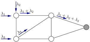
(a) Optimum forwarding for logarithmic cost function.

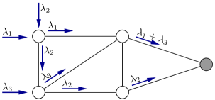
(b) Optimum forwarding for cubic cost function.

Energy Profile	Cost Function	Total Cost for Figure 1(a)	Total Cost for Figure 1(b)
Logarithmic	$c_{\ell}(\rho)=\log_{10}(1+\rho)$	0.65	0.85
Cubic	$c_{\ell}(\rho)=\rho^{3}$	1.33	0.48

Figure 1: Power saving routing example for three flows $\lambda_{1}=\lambda_{2}=\lambda_{3}=1$ with a common destination (the gray node). Every link has the same cost function (logarithmic or cubic) and $\mu_{\ell}=3\,\forall\ell\in\Lambda$.

There is an example in Figure 1 that shows feasible solutions to this problem for two different cost functions in a simple five nodes network. This elementary example illustrates how the different cost functions lead to distinct optimum forwarding strategies.

In the form above, the optimization problem is a generalization of the unsplittable multicommodity flow problem (UFP), where the generalization consists in allowing arbitrary cost functions $c_{\ell}(\cdot)$ for the links. With linear costs, (4)–(5c) is the classical UFP, which in specific instances is known to be NP-hard: for example, when the network $G$ has only one edge, the classical UFP specializes to the knapsack problem.

For general link-cost functions, the relaxation of the problem (4)–(5c) to $a(f,\ell)\in[0,1]$, namely to flows splitable over several routes, is generally a global minimization problem. The case when $c_{\ell}(\cdot)$ are concave functions is, for instance, NP-hard [30, 31]. Since we do not impose any prior assumption about the energy-consumption profiles, our problem can be regarded NP from a computational perspective.

Our final goal is to design a new routing algorithm that solves (4). The solution must be distributed and put low requirements on the network nodes. Additionally, it must be able to dynamically adapt to changing traffic demands and do so in a progressive manner, such that the changes in the set of network paths do not lead the network to a congested state nor cause undesired oscillations.

4 Routing Algorithm

As already stated in the introduction, we opt for a heuristic approach to solve the aforementioned NP-hard optimization problem. Among all the families of heuristic solvers available in the literature, the set of ant colony algorithms [22] maps almost directly to the problem at hand. Furthermore, their decentralized nature and time-adaptive characteristics are requisites for any deployable solution. Note that we do not propose how the routing decisions can be implemented in practice, although it is certainly feasible on a MPLS [32] network where RSVP-TE [33] takes the job of setting up the label switched paths (LSPs).

As in the seminal AntNet algorithm [22], our algorithm relies on autonomous agents (ants) that travel the network gathering enough information to form optimal paths. Agents travel the network from source to destination and back to the source. In their forward path, they explore different routes to the destination to measure their costs. In their return path, they update statistics at every node related to the fitness of the next-hop node chosen in the previous forward way. The per-flow routing table is finally calculated as the most appropriate next-hop for a given destination at every node.

While the original AntNet algorithm used path delay as the cost function, we use the power consumption. Moreover, AntNet only obtains a single path to a destination from a given core node, while our algorithm must be able to calculate different routes for every flow traversing each core node. This complicates the problem as now the cost of the links does not depend on the amount of traffic being carried by them in a linear way, and so it is important to consider individual routes for every flow, even when they share a common intermediate node and destination. Throughout the rest of this section, we detail how agents work and what information they collect to obtain the set of optimal paths for each flow that minimize global power consumption.

4.1 Information Gathering

A key part of the algorithm relies on obtaining enough information about the network state for updating the flow routes. It is the job of a forward agent to gather this information with the help of the network nodes.

For this, a forward agent departs periodically from the source node $o$ towards the flow destination $d$. This agent carries information about the current flow rate ($\lambda_{f}$) and the current flow path ($p_{\mathit{f}}$). The agent walks the network towards the flow destination in a non-deterministic manner to be detailed later. When the agent reaches a new node, it records the identity of the node in an internal list of visited nodes. At the same time, the agent calculates the marginal cost of carrying the flow traffic across the link used in the last hop and stores it internally as $\vec{c}^{f}[i]$, with $i$ the index of the previous node. This depends on the cost function of the link, the traffic already being carried by the link and whether the link is part of current flow path. The exact procedure to calculate the marginal cost is shown in Listing 1 (see function calcCost). Note that forward agents simply need that core nodes maintain statistics about aggregate traffic load in their outgoing links to calculate the marginal cost.

⬇

1calcCost = function($\ell$, $\lambda_{f}$, $p_{f}$, $\lambda_{\ell}$, $\mu_{\ell}$) {

2 if ($\ell\in$ $p_{f}$) { /* link belongs to the current path of flow $f$ */

3 /* Traffic in the link not from our flow */

4 $\lambda_{r}$ = $\lambda_{\ell}$ - $\lambda_{f}$;

5 } else {

6 /* No traffic is from our flow */

7 $\lambda_{r}$ = $\lambda_{\ell}$;

8 }

9 origCost = $c_{\ell}\left(\lambda_{r}/\mu_{\ell}\right)$;

10 newCost = $c_{\ell}\left((\lambda_{r}+\lambda_{f})/\mu_{\ell}\right)$;

11

12 return newCost - origCost;

13}

Listing 1: Procedure for the marginal cost calculation.

Before leaving the current node, forward agents need to decide which neighbor node to visit next. There is a trade-off in this selection, because agents should explore all the possible paths, but, at the same time, more resources should be used to explore good paths, where a good path is the one that the agent knows that demands less power than others. To achieve a balance in this selection, forward agents use two procedures to select the next visited node: one completely random using no previously obtained information, and the other one based on costs calculated by other agents. Which procedure to use is selected at random too. With some small probability $\pi_{e}$ the agent chooses the first procedure ensuring that eventually all possible routes are explored. With probability $1-\pi_{e}$ the next node is chosen according to its goodness relative to the flow $f$. There is a vector $\vec{G}_{i}(f)$ at every node $i$ that stores the goodness values for each flow $f$ to all neighboring nodes. That is, $\vec{G}_{i}(f)=\{g_{i}^{f}(j)\,\,\forall j\,|\,(i,j)\in\Lambda\}$. The goodness of each node is a probability related to the estimated power consumption of the flow should it select the neighbor node as part of its path. It must be stored in the nodes where it is updated by the backward agents.

Finally, if a cycle is detected after arriving to a new node, all the information about the nodes visited and the links traveled since the previous visit is deleted from the agent. A pseudo-code version of the algorithm governing forward agents is provided in Listing 2.

⬇

1for each $f(o,d,\lambda_{f})\in\Phi$ {

2 $F_{o\rightarrow d}$ = new ForwardAgent($f(o,d,\lambda_{f})$, $p_{f}$);

3 sendAgent($F_{o\rightarrow d}$);

4}

5

6sendAgent = function($F_{o\rightarrow d}$) {

7 i = o;

8 V = {}; // Set of visited nodes

9 $\vec{c}$ = []; // Vector holding the link costs

10

11 do {

12 j = nextNode($G_{i}(f)$);

13 $\ell$ = (i, j);

14 if (i $\in$ V)

15 purgeCycle(V, $\vec{c}\,$);

16 V = V $\cup$ i;

17 /* $\hat{\lambda}_{l}$ is the estimated amount of traffic carried by link $\ell$ */

18 $\vec{c}\,[\text{i}]$ = calcCost(l, $\lambda_{f}$, $p_{f}$, $\hat{\lambda}_{l}$, $\mu_{\ell}$);

19 i = j; // Visit the next node

20 } while (i != d);

21}

Listing 2: Forward agent algorithm.

4.2 Information Dissemination

The information gathered by the forward agent on its way to the destination node (the marginal costs and the path actually traversed) is used to update the goodness values at each of the intermediate nodes. The backward agent is in charge of this update process while it travels back to the origin node following exactly the reverse route recorded by the forward agent.

At an intermediate node $i\in N$ in the route of the backward agent from the destination $d$ toward the origin $o$, the goodness value is updated based on the cost of the partial path followed before by the forward agent from $i$ to $d$. In turn, this cost is the sum of two components: a direct cost that results from the addition of the flow’s traffic to the downstream links from $i$ on the path, and an indirect cost that measures the impact on the costs that the remaining flows would see should the current flow $f$ departs partially or totally from its current route.

1. The direct cost is computed directly from the measurements taken by the forward agent as

   $$C^{f}_{\text{direct}}(i)=\sum_{k=i}^{d}\vec{c}^{f}[k],$$ (6)

   where $d$ is the flow destination and $\vec{c}^{f}[k]$ is the vector of measures recorded by the forward agent at node $k$.

2. When a flow leaves or changes its route, this might actually induce an increase in the marginal costs of other flows that were sharing the same links, particularly if the energy profile in those links is sub-linear. This possible increment is thus regarded as the indirect cost of the partial route from $i$ to $d$ used by the forward agent. Specifically, the indirect cost is initialized at the destination $d$ when a backward agent is created, with value

   $$C_{\text{indirect}}^{f}(d)=\sum_{\ell\in p_{f}}\vec{\gamma}^{f}[\ell]$$ (7)

   where

   $$\vec{\gamma}^{f}[\ell]\triangleq\left(c_{\ell}(\lambda_{\ell}-\lambda_{f})+c_{\ell}(\lambda_{f})-c_{\ell}(\lambda_{\ell})\right)^{+}$$ (8)

   is the sum of the marginal increases in energy consumption of all other flows traversing the link if the flow $f$ were to leave link $\ell$, and $\lambda_{\ell}$ is the total traffic carried by link $\ell$. Writing $\lambda_{r}\triangleq\lambda_{\ell}-\lambda_{f}$ for the remaining traffic that stays in the link after the departure of flow $f$, the cost change (8) is simply the difference between the cost due to the remaining traffic $c_{\ell}(\lambda_{r})$ and the cost savings of shifting $\lambda_{f}$ units of traffic off its current operating point, i.e., $c_{\ell}(\lambda_{\ell})-c_{\ell}(\lambda_{f})$. The value of $\vec{\gamma}^{f}[\ell]$ is not allowed to be negative, as would happen for links with super-linear (convex) cost functions, in order to disincentivize that the flows change prematurely their paths. Such changes could lead to undesirable route flapping and network instability.

   The values of the vector $\vec{\gamma}^{f}$ are computed by the backward agent, for every visited link, as part of its reverse path. $\vec{\gamma}^{f}$ is stored at the source node of the flow, and it is carried by the forward agents to be used in the next round of the backward agents as follows: when the backward agent leaves node $j$ to visit node $i$, the indirect cost is updated

   $$C^{f}_{\text{indirect}}(i)=\begin{cases}C^{f}_{\text{indirect}}(j)-\vec{\gamma}^{f}[(i,j)],\quad&\text{if $(i,j)\in p_{f}$}\\ C^{f}_{\text{indirect}}(j),\qquad&\text{otherwise}.\end{cases}$$ (9)

   Therefore, the indirect cost decreases toward the source, and diminishes by an amount equal to the cost of leaving the links upstream from $i$ that flow $f$ really uses. As a result of this computation, the paths in which the departure of a flow $f$ would produce a larger cost to other concurrent flows are penalized in comparison to paths where this does not occur.

The sum of the direct and indirect costs is the raw goodness value computed by the backward agent before leaving its current node, and stored there

$$\Gamma^{f}(i)=C^{f}_{\text{direct}}(i)+C^{f}_{\text{indirect}}(i).$$ (10)

The goodness is used as a metric to select the best next-hop for every flow. To this end, it is essential that paths with less energy demands yield increasing goodness, but this condition is not guaranteed for the raw goodness for a number of reasons. The raw values are noisy due to the measurement process, and have to be normalized first for allowing the comparison with the values computed by other backward agents for the same flow, possibly after having explored different paths. Finally, some adjustment is needed to ensure that the metric is monotonically decreasing in $\Gamma^{f}[i]$. In this paper, we will apply the same mechanisms and problem-independent constants as [21] to derive the routing metric.

To simplify notation, we set $\Gamma=\Gamma^{f}(i)$ for the rest of this Section. First, $\Gamma$ is normalized by a scaled average of previous measurements

$$r^{\prime}=\min\{\frac{\Gamma}{\alpha\overline{\Gamma}},1\}$$ (11)

where $\alpha>1$ is a suitable attenuation constant and $\overline{\Gamma}$ denotes the average of past samples of $\Gamma$. Averaging smoothes the measurements and reduces the variance, but this variance can still be high and trigger instability in the routing decisions. Thus, $r^{\prime}$ is corrected according to

$$r^{\prime}_{a}=\begin{cases}r^{\prime}-\textrm{e}^{-\frac{a\sigma}{\overline{\Gamma}}}\quad&\text{if $r^{\prime}<0.5$}\\ r^{\prime}+\textrm{e}^{-\frac{a\sigma}{\overline{\Gamma}}}\quad&\text{otherwise}\end{cases}$$ (12)

where $\sigma$ stands for the standard deviation of $\Gamma$. This correction is enforced only if the average $\overline{\Gamma}$ is considered reliable, i.e., if the ratio $\sigma/\overline{\Gamma}<\epsilon\ll 1$. If the average is not stable, $\sigma/\overline{\Gamma}\geq\epsilon$ then a penalty factor is added

$$r^{\prime}_{a}=\begin{cases}r^{\prime}+1-\textrm{e}^{-\frac{b\sigma}{\overline{\Gamma}}}\quad&\text{if $r^{\prime}<0.5$}\\ r^{\prime}-1-\textrm{e}^{-\frac{b\sigma}{\overline{\Gamma}}}\quad&\text{otherwise}\end{cases}$$ (13)

where $b<a$. Finally, the metric $r^{\prime}_{a}$ is compressed via the power law $r^{\prime}_{a}\leftarrow(r^{\prime}_{a})^{h}$ and clipped to the interval $[0,1]$.

After these nonlinear recalibration steps, node $i$ computes the goodness routing metric to each of its neighbors $j\in N$, $(i,j)\in\Lambda$ as follows:

$$g_{i}^{f}(j)\leftarrow g_{i}^{f}(j)+\begin{cases}(1-r^{\prime}_{a})\bigl{(}1-g_{i}^{f}(j)\bigr{)}\quad\text{agent comes from $j$}\\ -(1-r^{\prime}_{a})g_{i}^{f}(j)\quad\text{otherwise}.\end{cases}$$ (14)

It is easy to check that if $\sum_{j\in N,(i,j)\in\Lambda}g_{i}^{f}(j)=1$ then the same condition holds after applying the update rule (14), so $g_{i}^{f}(j)$ can be conveniently interpreted as the likelihood of preferring neighbor $j$ as the next hop. A total goodness of $1$ is easily enforced by choosing as initial values $g_{i}^{f}(j)=1/n_{i}$ for every neighbor $j$ of node $i$, with $n_{i}$ adjacent nodes. Therefore, in absence of better a priori information, initially each neighbor receives the same goodness as a credit.

4.3 Obtaining the New Path

Once the new goodness values have been calculated, the backward agent selects the maximum as the next hop for the flow. This information is stored internally by the agent.

When the agent finally reaches the source node for the flow, the information about the next hops is employed to construct a new path. Because the backward agent follows the reverse path of the forward agent, and the newly constructed path is just the ordered collection of best next nodes, as determined by their respective goodness values, for the visited nodes, this new path is not necessarily connected. So before replacing the current path, the origin node performs a connectivity test on it. For this, it can either rely on an existing link state routing algorithm or send any kind of source routed probe packet.

Even if the recorded path is dismissed, the work done by the agents is not lost. Chances are high that a new forward agent eventually follows the best path, as it is the one with the highest goodness values at every node, and thus, the resulting backward agent will record the whole path.

4.4 Memory Requirements

It is important to characterize the memory requirements for storing all the information related to the state of the agents and any auxiliary information they may need. To this end, we detail the memory needs of edge nodes, regular nodes and agents. Obviously, since agents are not physical entities, they cannot really store any information, so they store it transiently in the nodes they visit. In any case, we account for this separately from the memory needs of regular nodes for clarity.

The forward agent carries the following information: a set of visited nodes, the cost of the traveled links, the flow rate, the current path, and the extra cost of leaving links in the current path. That is, information about the current path and the traveled one. All this information depends solely on the path lengths, and so it usually scales with the logarithm of the number of nodes.

The backward agent does not carry much more information than the forward one. It just stores the current path and, additionally, the extra cost values of those links traveled that are part of the current path. Finally, it also holds a copy of the path followed by the forward agent and it records the best next hop node for the visited nodes. Again, all this information is proportional to the path length, so it is independent of the number of flows.

The agents do use information stored in the nodes to communicate with other agents and to obtain some basic information for their calculations. Source nodes must store for every flow originating from them the current path of the flow, its rate and the extra cost incurred when the flow leaves any of the links currently traversed. The rate information scales linearly with the number of flows departing from the node, while the path information and extra costs scales with the product between the number of flows departing at the node and the logarithm of the network size. We consider as a single flow all traffic between a given pair of edge nodes, the total information stored at the edges is still manageable. In the worst case, it is $|E|\log(N)$, with $|E|$ the number of edge nodes.

Regular nodes, and edge nodes too, need to store additional information for the agents to do their calculations. They need an estimate of the traffic being sent across every outgoing link for the cost calculation. They also need to store the information for the best node selection: the goodness vector and the cost statistics for each flow. Each goodness vector has an entry for every outgoing link ($\frac{2|\Lambda|}{|N|}$ on average), so its size should remain relatively small. However, the node must store a goodness vector for every network flow. In the worst case, there can be as many as $|E|(|E|-1)$ flows in the network, so this is clearly the limiting factor of the algorithm. To lower this memory requirement, nodes could use some kind of eviction policy to free memory associated to flows without recent activity. All this information is summarized in Table 2.

Element	Needed storage
Forward agent	$O(\log(N))$
Backward agent	$O(\log(N))$
Source node	$O(|E|\log(N))$
Core node	$O\left(\frac{2|\Lambda|}{|N|}|E|^{2}\right)$

Table 2: Memory requirements.

5 Evaluation

In this section we will analyze the performance of our algorithm. We start with a set of simple experiments in a synthetic topology that highlights the behavior of the algorithm for different cost functions. Then, we show the results on more realistic network topologies.

All the results have been produced by an open source in-house simulator available at [34]. Our simulator abstracts packet level simulation details and considers the long time traffic averages known. This speeds up the simulations while, at the same time, let us employ publicly available traffic matrices that do not usually detail packet level details. The simulator reads two configuration files: one describes the network topology and link parameters and the second one controls the traffic characteristics. The simulated links are described by their maximum traffic capacity and their cost function. The cost function for a given link is reduced for simplicity to the set of coefficients $\{a_{0},\ldots,a_{n}\}$ in the general formula

$$c_{\ell}(\lambda)=a_{0}\log\lambda+\sum_{i=1}^{n}a_{i}\lambda^{i-1}.$$ (15)

This formula lets us represent the main power profiles links are expected to exhibit in the near future [19, 25]: sub-linear, like those of IEEE 802.3az links [4]; linear (although this is not expected to be found in links, it can be used to account for the power costs of the switch matrix of the routers), a constant component, although this does not have any effect on the routing decisions, and super-linear. These latter profiles, like cubic ones, have been found in Ethernet interfaces applying dynamic voltage and frequency scaling [36]. Finally, we do not consider an on-off power profile as we need all links to be active to be able to send and receive agents through them. In any case, with a suitable scaling factor, the logarithmic profile can be made similar to the on-off profile. For the algorithm configuration parameters, we used the constants provided in [22]: $\epsilon=0.25$, $a=10$, $b=9$ and $h=0.04,$ that are problem independent. In any case, it has been found that Ant Colonization algorithms are quite resilient to changes in the configuration parameters [37], so further tuning has not been deemed necessary.

Given the inherent random behavior of the algorithm, each simulation has been repeated 100 times, modifying the initial seed of the random generator of the simulator. All the provided results show the averaged measure of a given metric along with its 95 % confidence interval, except in those cases where the interval was too small.

5.1 Algorithm Behavior

The first set of results shows the behavior of the algorithm in a regular network. The topology consists of a simple switching matrix of $n$ steps connecting $n$ traffic sources to $n$ destinations. Every link has the same cost function and unlimited capacity. The goal is to check the results obtained by the algorithm in an otherwise unrestricted scenario. Traffic consists of $n$ identical flows going from each source to every destination, for a total of $n^{2}$ flows in the network.

Figure 2: Algorithm behavior in a lattice network with a logarithmic cost function. Line width represents the number of flows in a link, while dotted lines show unused links.

Figure 3: Algorithm behavior in a lattice network with a cubic cost function.

Figure 4: Algorithm behavior in a lattice network with a linear cost function.

Figures 2, 3 and 4 show a graphical representation of the network and the link occupations for $n=5$ and three different cost functions: logarithmic, cubic and linear, respectively. The number of flows in each link is proportional to the line width, with dotted lines representing unused links. After a close inspection of the graphics it can be seen that in the logarithmic scenario (Figure 2), routes tend to be short (vertical links are only used in the first and final steps) and shared among various flows. Note that line widths are quite wide and, at the same time, a lot of links remain unused. This is expected, as the marginal cost of adding traffic to a link decreases with its load.

In contrast, for the cubic cost function (Figure 3), most links are lightly used. In fact, almost all vertical links are employed to avoid sharing traffic on either horizontal or diagonal links. Again, this is the expected behavior, as in this case the marginal cost increases with load, so the algorithm must find the way to spread the traffic across the net as long as the added cost (it employs more links and longer routes) is not excessive.

In the linear scenario (Figure 4) the algorithm just searches for the shortest routes regardless of how the links are shared among flows. As in the logarithmic cost function scenario, there is almost no single vertical link used, but it can be also observed that the load is not so concentrated on a few links. In fact, the total number of empty links is smaller.

We repeated these simulations on a somewhat larger net with $n=8$.

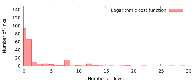
(a) Logarithmic cost function

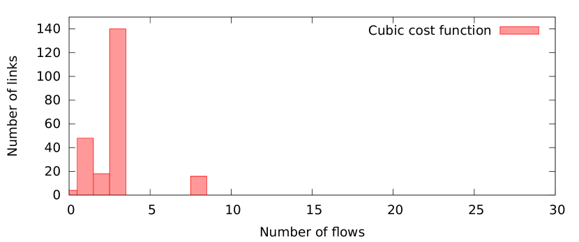
(b) Cubic cost function

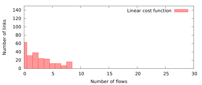
(c) Linear cost function

Figure 5: Link occupation for an 8-nodes regular topology for different cost functions.

Figure 5 shows how many links share a given number of flows. Results agree with the above discussion. The logarithmic scenario has the highest number of unused links (96) with some links carrying 27 or even 29 flows. On the contrary, for the cubic cost function most links carry just a few flows with almost no link sitting unused. The linear case, as before, fits in between those scenarios.

	Ant Colonization Algorithm			SPF
Cost Function	Log	Linear	Cubic	Any
Path Length	$9.9\pm 0.6$	$9$	$9.9\pm 0.1$	9
Energy Savings	$13.3\pm 1.3\,$%	$0\,$%	$69.9\pm 0.1\,$%	$0\,$%

Table 3: Energy savings and path lengths obtained for different cost functions in a regular switching network with $n=8$. $95\,$% confidence interval omitted for clarity when less than $0.1\,$%.

Finally, the results obtained after the algorithm is run are summarized in Table 3. It shows both the energy savings when compared to a power unaware shortest-path-first (SPF) routing algorithm and the average route lengths. As expected, for the linear cost function, the results are identical to those of the SPF algorithm, and thus our algorithm produces no energy savings, but keeps the optimum average path length of just nine hops. However, for non-linear cost functions it pays a small penalty in path lengths. This length increment is necessary to obtain more power efficient routes. In fact, the energy savings for the cubic cost function ($69.9\pm 0.1\,$%) are quite impressive in this topology.

5.2 Performance Results

We have also carried out experiments in more realistic network topologies, the first set inspired in the topology of the old NSFNet network and a second one in the nobel-eu topology from the Survivable Network Design Library (SNDlib) [38].

Figure 6 shows the NSFNet network. We have conducted several simulations with varying traffic matrices: a full-mesh matrix with traffic flowing from each source to every other destination; an intra-coast matrix, with traffic just between some nodes in the same “coast”; and finally a coast-to-coast matrix, with traffic flowing from nodes in each coast to the other and vice-versa.

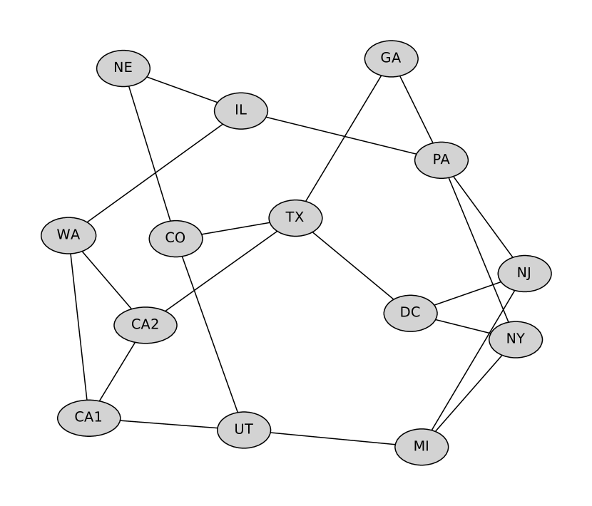
Figure 6: Network topology based on the original NSFNet. Node names correspond with their geographic location.

Although the traffic matrices can not be considered real by any means, they allow to bring some light to the behavior and performance of the algorithm in a wide range of representative scenarios.

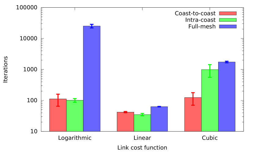
Figure 7: Number of iterations to reach 90% of the greatest power savings for different traffic matrices and different link cost functions. Error bars show 95 % confidence intervals.

The first performance characteristic we measured is the time needed by the algorithm to reach $90\,$% and $99\,$% of the long term energy savings it is able to achieve. We use the number of iterations, that is, the number of forward agents sent by a source, as a proxy for this time, as it eventually depends on the time separation between two consecutive agents. The results are plotted in Figures 7 and 8.

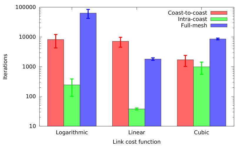
Figure 8: Number of iterations to reach 99% of the greatest power savings for different traffic matrices and different link cost functions. Error bars show 95 % confidence intervals.

The first conclusion is that the algorithm is usually able to reach the target of $90\,$% quite fast. There is also a relationship between the number of flows and the convergence speed. This can be observed in the full mesh simulations, which usually take the largest number of iterations. It can also be seen that the intra-coast scenario is resolved very fast for any cost function, as it takes almost the same number of iterations to reach $90\,$% of the final savings as to get to $99\,$%. We believe that this is a consequence of the optimal routes being quite short, and thus easy to come across by the agents. On the other hand, both the coast-to-coast and the full-mesh matrices need many more iterations to rise to the $99\,$% target. For the linear cost function this happens because the optimal routes are longer and thus the number of alternative routes with similar costs is higher, lowering the likelihood of a forward agent to follow them. The change for the logarithmic cost function is even sharper. The reason is that not only the routes are longer, like in the linear case. There is an additional complexity in the fact that the algorithm tries to pack several flows in the same links for maximum energy savings. As the agents take their routing decisions autonomously it takes some extra time for routes to converge to the same set of links. This also helps to explain why for the cubic cost function the complexity increase is less noticeable. For super-linear cost functions the greatest savings come from using disjoint routes, so there is no need for several flows to converge on the same set of links. So, it is easier for agents to choose links with low occupation.

We have also measured two additional performance characteristics: actual power savings and average path length increment. The power savings are compared to the power consumed by a network using SPF as the power-agnostic routing algorithm.

		Cost Function
		Log	Linear	Cubic
Length	Coast to coast	$20.1\pm 1.1\,$%	$0\,$%	$16.1\pm 1.2$ %
Increment	Intra coast	$23.3\pm 1.9\,$%	$0\,$%	$0\,$%
	Full mesh	$11.0\pm 0.6\,$%	$0\,$%	$0.8\pm 0.1\,$%
Relative	Coast to coast	$29.5\pm 1.2\,$%	$0\,$%	$17.6\pm 1.3\,$%
energy	Intra coast	$6.5\pm 1.4\,$%	$0\,$%	$0\,$%
savings	Full mesh	$29.9\pm 0.5\,$%	$0\,$%	$12.8\pm 0.06\,$%

Table 4: Performance improvement of the proposed algorithm for different traffic matrices in the network depicted in Figure 6 when compared against Shortest Path First. $95\,$% confidence intervals omitted for clarity when less than $0.1\,$%.

The results for the three traffic matrices and the three power profiles are summarized in Table 4. For the linear cost function, the algorithm is unable to save more energy with regards to SPF, but this is expected, as SPF discovers the optimal routes for these networks. In any case, the results of our algorithm are also optimal, with no additional energy demands nor increments in the path lengths.

In the logarithmic link cost networks, the algorithm obtains more than $20\,$% energy savings for the more complex traffic matrices. The route lengths also grow, although the increments are below $25\,$%.

Finally, the cubic cost function does not attain any savings for the intra-coast traffic matrix. This is because the shortest path routes are already optimal. In fact, the path lengths are identical for both the proposed algorithm and the SPF routing algorithm. For the rest of the traffic matrices it gets savings in the $10$–$20\,$% range by distributing flows in different links, at the cost of an obvious increment in the average path length.

In short, the proposed algorithm is able to trade some increment in route lengths to save energy in the network. When the routes computed by a shortest path first algorithm are already optimal, the routes computed by our proposal are never worse: both average path length and energy consumption remain identical.

As already stated at the beginning of the Section, we have also used a real topology both to assess the behavior of our algorithm and to compare it against the optimization shown in [20, 26] and to those power profile unaware algorithms that minimize the number of active links [14, 9, 23, 24]. We have employed the topology and average traffic matrix of the nobel-eu core network from the SNDlib archive used in those works. The nobel-eu network is a European network consisting on 28 nodes connected by 41 links and the traffic matrix consists on a total of 378 flows. For the sake of the comparison, we have simplified the network model proposed in [26] as we restrict the number of links between a given pair of nodes to one, albeit with unlimited capacity.

Figure 9 shows the normalized power consumption with a cubic cost function.

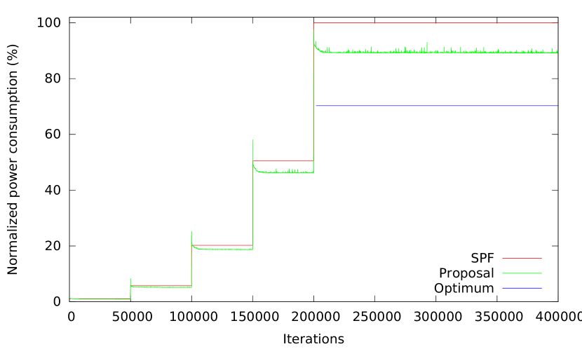
Figure 9: Comparison between our algorithm, SPF and the optimal result for the nobel-eu network with a cubic cost function.

Traffic was added to the network in several steps to show the dynamics of our algorithm. It can be seen that the consumption raises briefly above that of SPF when new traffic enters the network, but rapidly stabilizes below it after a few iterations. For completeness we have calculated with the help of the IBM CPLEX solver the optimum power consumption obtained considering our simplified model of [26]. As expected, the centralized calculation is able to obtain the best results, albeit it cannot adapt automatically to changing network conditions. We also performed the experiment with a logarithmic cost function. In this case, our algorithm just managed to save $3\pm 1\,\%$ of the power needed when using SPF routes, while the CPLEX solver managed to save 16% of the power, considering again a static scenario.

To simulate the results of the power profile unaware algorithms we eliminated all but the most used outgoing link for each node when using SPF routing. Then, we calculated the global power usage in the modified graph. We found that energy usage increases $9.5\,$% for links with logarithmic cost function when compared with the unmodified network using SPF as a routing algorithm. This is due to the increased average length of the routes, resulting in traffic consuming energy in more links. Results, however, are much worse for a cubic cost function. In this case, traffic should be spread over various links to minimize consumption, however, with a single path between each pair of nodes this is not feasible. Energy consumption is $8.8\,$ times higher than in the unmodified network. Although the results may seem counter intuitive, there are to be expected, as all these algorithms are designed for networks with fixed cost links.

6 Conclusions

In this paper we have presented a modified version of the AntNet [22] algorithm to calculate, in a decentralized way, optimal routes to reduce power consumption of network links. The presented solution does not put any restriction in the power profile functions of the networking equipment.

The proposal was tested in both synthetic and real scenarios with different power profiles. The obtained results show power savings in the 10–20% range for real networks and up to 70% in favorable, although unlikely, scenarios. Moreover, the convergence times are small, as the 90% of the savings are usually obtained in less than 1000 iterations. Thus the algorithm can be used continuously in background in the network, adapting the routing tables to the medium-term averages of the traffic load of the incoming flows.

Finally, the results also show that it is necessary to take into account the power profile of the links, as not doing so and blindly powering off less used links can even augment power usage.

References

- [1] S. Lanzisera, B. Nordman, R. E. Brown, Data network equipment energy use and savings potential in buildings, in: ACEEE Summer Study on Buildings, 2010.
-
[2]
The Climate Group,
SMART 2020.
Enabling the low carbon economy in the information age, Tech. rep., Global
e-Sustainibility Initiative (GeSI), accessed July 30 2014
(2008).
URL http://smart2020.org/_assets/files/02_Smart2020Report.pdf - [3] P. Reviriego Vasallo, J. A. Hernández, D. Larrabeiti, J. A. Maestro, Performance evaluation of Energy Efficient Ethernet, IEEE Communications Letters 13 (9) (2009) 697–699.
- [4] S. Herrería Alonso, M. Rodríguez Pérez, M. Fernández Veiga, C. López García, A GI/G/1 model for 10 Gb/s energy efficient Ethernet, IEEE Transactions on Communications 60 (2012) 3386–3395. doi:10.1109/TCOMM.2012.081512.120089.
- [5] V. Sivaraman, P. Reviriego, Z. Zhao, A. Sánchez-Macián, A. Vishwanath, J. Maestro, C. Russell, An experimental power profile of energy efficient ethernet switches, Computer Communications 50 (2014) 110 – 118, green Networking. doi:10.1016/j.comcom.2014.02.019.
- [6] M. I. Khan, W. N. Gansterer, G. Haring, Static vs. mobile sink: The influence of basic parameters on energy efficiency in wireless sensor networks, Computer Communications 36 (9) (2013) 965 – 978, reactive wireless sensor networks. doi:10.1016/j.comcom.2012.10.010.
- [7] D. Jung, R. Kim, H. Lim, Power-saving strategy for balancing energy and delay performance in {WLANs}, Computer Communications 50 (2014) 3 – 9, green Networking. doi:10.1016/j.comcom.2014.02.005.
- [8] M. Gupta, S. Singh, Greening of the Internet, in: SIGCOMM ’03: Proceedings of the 2003 conference on Applications, technologies, architectures, and protocols for computer communications, ACM, 2003, pp. 19–26.
- [9] L. Chiaraviglio, M. Mellia, F. Neri, Minimizing ISP network energy cost: Formulation and solutions, IEEE/ACM Transactions on Networking 20 (2) (2012) 463–476. doi:10.1109/TNET.2011.2161487.
- [10] M. Caria, A. Engelmann, A. Jukan, B. Konrad, How to slice the day: Optimal time quantization for energy saving in the Internet backbone networks, in: Global Communications Conference (GLOBECOM), 2012 IEEE, 2012, pp. 3122–3127. doi:10.1109/GLOCOM.2012.6503594.
- [11] J. F. Botero, X. Hesselbach, M. Duelli, D. Schlosser, A. Fischer, H. de Meer, Energy efficient virtual network embedding, IEEE Communications Letters 16 (5) (2012) 756–759. doi:10.1109/LCOMM.2012.030912.120082.
- [12] B. Addis, A. Capone, G. Carello, L. Gianoli, B. Sanso, Energy management through optimized routing and device powering for greener communication networks, Networking, IEEE/ACM Transactions on 22 (1) (2014) 313–325. doi:10.1109/TNET.2013.2249667.
- [13] A. Cianfrani, V. Eramo, M. Listanti, M. Marazza, E. Vittorini, An energy saving routing algorithm for a green OSPF protocol, in: INFOCOM IEEE Conference on Computer Communications Workshops , 2010, 2010, pp. 1–5.
- [14] A. Cianfrani, V. Eramo, M. Listanti, M. Polverini, A. V. Vasilakos, An OSPF-integrated routing strategy for QoS-aware energy saving in IP backbone networks, IEEE Transactions on Network and Service Management 9 (3) (2012) 254–267. doi:10.1109/TNSM.2012.031512.110165.
- [15] IEEE 802.3az (Oct. 2010). doi:10.1109/IEEESTD.2010.5621025.
- [16] J. Zhang, N. Ansari, Toward energy-efficient 1G-EPON and 10G-EPON with sleep-aware MAC control and scheduling, IEEE Communications Magazine 49 (2) (2011) s33–s38. doi:10.1109/MCOM.2011.5706311.
- [17] M. Rodríguez Pérez, S. Herrería Alonso, M. Fernández Veiga, C. López García, Improving energy efficiency in upstream EPON channels by packet coalescing, IEEE Transactions on Communications 60 (4) (2012) 929–932. doi:10.1109/TCOMM.2012.022712.110142A.
- [18] A. Bianco, F. G. Debele, L. Giraudo, On-line power savings in a distributed multi-stage router architecture, in: Global Communications Conference (GLOBECOM), 2012 IEEE, 2012, pp. 2535–2540. doi:10.1109/GLOCOM.2012.6503498.
- [19] J. C. Cardona Restrepo, C. G. Gruber, C. Mas Machuca, Energy profile aware routing, in: Communications Workshops, 2009. ICC Workshops 2009. IEEE International Conference on, 2009, pp. 1–5.
- [20] R. G. Garroppo, S. Giordano, G. Nencioni, M. Pagano, Energy aware routing based on energy characterization of devices: Solutions and analysis, in: Communications Workshops (ICC), 2011 IEEE International Conference on, 2011, pp. 1–5. doi:10.1109/iccw.2011.5963560.
- [21] I. Seoane, J. Hernandez, P. Reviriego, D. Larrabeiti, Energy-aware flow allocation algorithm for energy efficient Ethernet networks, in: Software, Telecommunications and Computer Networks (SoftCOM), 2011 19th International Conference on, 2011, pp. 1–5.
- [22] G. Di Caro, M. Dorigo, AntNet: A mobile agents approach to adaptive routing, Tech. rep., Université Libre de Bruxelles, IRIDIA 97–12 (Dec. 1997).
- [23] Y.-M. Kim, E.-J. Lee, H.-S. Park, J.-K. Choi, H.-S. Park, Ant colony based self-adaptive energy saving routing for energy efficient Internet, Computer Networks 56 (10) (2012) 2343–2354. doi:http://dx.doi.org/10.1016/j.comnet.2012.03.024.
- [24] Y. Yang, M. Xu, Q. Li, Towards fast rerouting-based energy efficient routing, Computer Networks 70, in press. doi:10.1016/j.comnet.2014.04.014.
- [25] L. Chiaraviglio, D. Ciullo, M. Mellia, M. Meo, Modeling sleep mode gains in energy-aware networks, Computer Networks 57 (15) (2013) 3051–3066.
- [26] R. Garroppo, G. Nencioni, L. Tavanti, M. G. Scutellà, Does traffic consolidation always lead to network energy savings?, IEEE Communications Letters 17 (9) (2013) 1852–1855.
- [27] A. Nazi, M. Raj, M. D. Francesco, P. Ghosh, S. K. Das, Deployment of robust wireless sensor networks using gene regulatory networks: An isomorphism-based approach, Pervasive and Mobile Computing 13 (2014) 246 – 257. doi:10.1016/j.pmcj.2014.03.005.
- [28] T. Lu, J. Zhu, Genetic algorithm for energy-efficient QoS multicast routing, IEEE Communications Letters 17 (1) (2013) 31–34. doi:10.1109/LCOMM.2012.112012.121467.
- [29] J. Galán Jiménez, A. Gazo Cervero, Using bio-inspired algorithms for energy levels assessment in energy efficient wired communication networks, Journal of Network and Computer Applications 37 (2014) 171–185. doi:10.1016/j.jnca.2013.02.027.
- [30] S. Sahni, Computationally related problems, SIAM Journal on Computing 3 (4) (1974) 262–279. doi:10.1137/0203021.
- [31] S. A. Vavasis, Quadratic programming is in NP, Inf. Process. Lett. 36 (2) (1990) 73–77. doi:10.1016/0020-0190(90)90100-C.
-
[32]
E. Rosen, A. Viswanathan, R. Callon,
Multiprotocol label switching
architecture, RFC 3031 (Jan. 2001).
URL http://www.ietf.org/rfc/rfc3031.txt -
[33]
RSVP-TE: Extensions to RSVP for
LSP tunnels, RFC 3209 (Dec. 2001).
URL http://www.ietf.org/rfc/rfc3209.txt -
[34]
M. Rodríguez Pérez, S. Herrería Alonso,
Trancas simulator (Mar. 2014).
URL http://migrax.github.io/trancas/ - [35] NS, ns Network Simulator, http://www.isi.edu/nsman/ns/ (Mar. 2007).
- [36] B. Zhai, D. Blaauw, D. Sylvester, K. Flautner, Theoretical and practical limits of dynamic voltage scaling, in: Proceedings of the 41st annual Design Automation Conference, DAC ’04, ACM, New York, NY, USA, 2004, pp. 868–873. doi:10.1145/996566.996798.
- [37] S. S. Dhillon, P. Van Mieghem, Performance analysis of the AntNet algorithm, Computer Networks 51 (8) (2007) 2104–2125. doi:10.1016/j.comnet.2006.11.002.
- [38] S. Orlowski, M. Pióro, A. Tomaszewski, R. Wessäly, SNDlib 1.0–Survivable Network Design Library, in: Proceedings of the 3rd International Network Optimization Conference (INOC 2007), Spa, Belgium, 2007, http://sndlib.zib.de, extended version accepted in Networks, 2009.