Steklov Mathematical Institute, Russian Academy of Sciences
Gubkina st. 8, Moscow, 119991, Russia

Abstract. In this paper, the dynamics of nonholonomic systems on Lie groups with a left-invariant kinetic energy and left-invariant constraints are considered. Equations of motion form a closed system of differential equations on the corresponding Lie algebra. In addition, the effect of change in the stability of steady motions of these systems with the direction of motion reversed (the reversal found in rattleback dynamics) is discussed. As an illustration, the rotation of a rigid body with a fixed point and the Suslov nonholonomic constraint as well as the motion of the Chaplygin sleigh is considered.

Keywords Lie group, left-invariant constraints, Euler – Poincaré – Suslov systems, Chaplygin sleigh, anisotropic friction, conformally Hamiltonian systems, stability

Mathematics Subject Classification (2000) 34D20, 70E40, 37J35

1 Euler – Poincaré – Suslov nonholonomic systems

Let the configuration space of a mechanical system with $n$ degrees of freedom represent a Lie group $G$, and let $w_{1},\ldots,w_{n}$ be independent left-invariant vector fields on $G$ (they are invariant under all left translations on $G$). The commutators of these fields have the form

$$[w_{i},w_{j}]=\sum\limits_{k=1}^{n}c_{ij}^{k}w_{k},$$ (1)

where $c_{ij}^{k}=-c_{ji}^{k}$ are the structure constants of $G$.

Let $x=(x_{1},\ldots,x_{n})$ be local (generalized) coordinates on $G$ and $f(x)$ be a smooth function. Then

$$\dot{f}=\frac{\partial f}{\partial x}\cdot\dot{x}=\sum\limits_{i=1}^{n}w_{i}(f)\omega_{i},$$

where $w_{i}(f)=\frac{\partial f}{\partial x}\cdot w_{i}$ is the derivative $f$ along the vector field $w_{i}$. The variables $\omega$ (called quasi-velocities) linearly depend on $\dot{x}$:

$$\dot{x}_{k}=\sum\limits_{i=1}^{n}w_{i}(x_{k})\omega_{i},\quad 1\leq k\leq n.$$ (2)

The quasi-velocities are Cartesian coordinates on the Lie algebra $g$ of $G$.

Assume that the Lagrangian of the system of interest is reduced to the kinetic energy $T$ which generates a left-invariant Riemannian metric $(\cdot,\cdot)$ on $G$. In this case

$$T=\frac{1}{2}\,(\dot{x},\dot{x})=\frac{1}{2}\Big{(}\sum w_{i}\omega_{i},\sum w_{j}\omega_{j}\Big{)}=\frac{1}{2}\sum I_{ij}\omega_{i}\omega_{j},$$

where

$$I_{ij}=(w_{i},w_{j})=\text{const},$$

since all the vector fields $w_{1},\ldots,w_{n}$ are left-invariant. The scalar-product matrix $\|I_{ij}\|$ is positive definite. This is the inertia tensor of the mechanical system.

According to Poincaré [12] (see also [1]), the Lagrange equations take the following form:

$$\dot{m}_{i}=\sum\limits_{j,k=1}^{n}c_{ji}^{k}m_{k}\omega_{j},\quad 1\leq i\leq n.$$ (3)

Here

$$m_{i}=\frac{\partial T}{\partial\omega_{i}}=\sum I_{ij}\omega_{j}$$

are the components of the angular momentum of the system; this is a vector from the linear space $g^{*}$ dual to $g$. Eqs. (3) are a closed system of differential equations with quadratic right-hand sides on $g$ (or on $g^{*}$). The system is often called Euler – Poincaré equations on a Lie algebra. For the group of rotations of the three-dimensional Euclidean space $SO(3)$, Eqs. (3) coincide with the Euler equations from rigid body dynamics. To completely describe the motion, one needs to add the kinematic equations (2) to Eqs. (3).

Now we increase the complexity of the problem by adding some constraints that are linear in the velocities and generally nonintegrable:

$$f_{1}(\omega,x)=\ldots=f_{m}(\omega,x)=0\quad(m<n).$$

Of particular interest is the case where, apart from the kinetic energy $T$, the functions of the constraints $f_{1},\ldots,f_{m}$ are also left-invariant (i. e., explicitly independent of $x$). Under this condition the nonholonomic Lagrangian equations with the constraints

$$\dot{m}_{i}=\sum\limits_{j,k=1}^{n}c_{ji}^{k}m_{k}\omega_{j}+\sum\limits_{p=1}^{m}\lambda_{p}\frac{\partial f_{p}}{\partial\omega_{i}},\quad f_{1}(\omega)=\ldots=f_{m}(\omega)=0$$ (4)

form a closed system of differential equations on the Lie algebra $g$.

For the case $G=SO(3)$ systems with left-invariant constraints were first studied by Suslov [25]. He considered the rotation of a rigid body about a fixed point with the following nonholonomic constraint: the projection of the angular velocity vector $\omega\in SO(3)=\mathbb{R}^{3}$ onto a body-fixed axis equals zero. General nonholonomic systems on Lie groups with a left-invariant kinetic energy and left-invariant constraints were studied in [20, 11]. These systems are called Euler – Poincaré – Suslov (EPS) systems. Since the constraints are linear in the velocity, Eqs. (4) admit the energy integral

$$T=\frac{1}{2}\sum I_{ij}\omega_{i}\omega_{j}=h=\text{const}.$$ (5)

In Suslov’s problem Eqs. (4) have the form

$$I\dot{\omega}+\omega\times I\omega=\lambda a,\quad(a,\omega)=0.$$ (6)

Here $a\neq 0$ is some constant vector in a moving space. If $a$ is an eigenvector of the inertia operator ($Ia=\rho a$, $\rho\in\mathbb{R}$), then it follows from (6) that $\omega=\text{const}$ (see [25]). In particular, all rotations of the rigid body are stable.

In a typical case (where this condition does not hold), each solution $t\,{\mapsto}\,\omega(t)$ possesses the following property:

$$\lim\limits_{t\to\pm\infty}\omega(t)=\pm\omega_{0}.$$ (7)

The motion of a rigid body is an asymptotic transition from steady rotation about some body-fixed axis to steady rotation with the same angular velocity about the same axis but in the opposite direction. We emphasize that in fixed space, as $t\to+\infty$ and $t\to-\infty$, these rotations occur about different axes. The angular velocities of the steady rotations (7) are found from the system (6). On the one hand, we have the constraint equation $(a,\omega_{0})=0$. On the other hand, performing scalar multiplication of the first equation (6) by $I\omega^{0}$, we obtain one more equation: $(Ia,\omega_{0})=0$. This yields all steady-state solutions of the system (6):

$$\omega_{0}=\mu a\times Ia,\quad\mu\in\mathbb{R}.$$ (8)

The phase portrait of the system (6) is shown in Fig. 1.

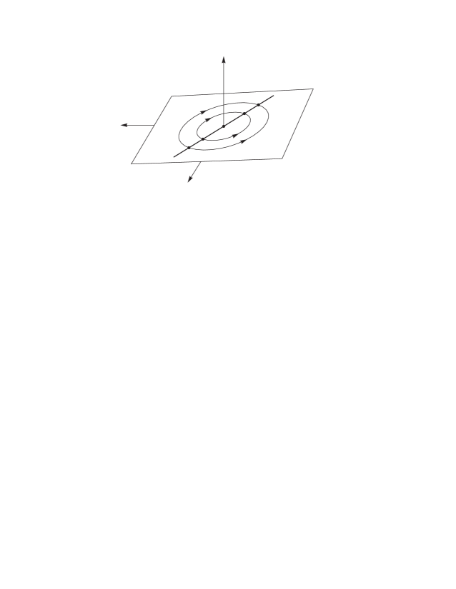
Fig. 1:

It is evident from this phase portrait that the phase flow of this system does not admit an invariant measure with a continuous (and even summable) density. The conditions for the existence of an invariant measure of the EPS equations (4) in the multidimensional case are given in [20]. Equality (7) holds also for Suslov’s problem in the $n$-dimensional space where $G=SO(n)$ [11] (see also [14, 10]).

The absence of an invariant measure prevents one from applying thegeometrical version of the Euler – Jacobi theorem which was formulated in [19, 2], although explicit quadratures can be obtained (see [25]). This motivated the development of an approach [15] based on the Hamiltonization of this system in open regions of the phase space. In [9], it is shown that under certain conditions the complete system in Suslov’s problem (including the evolution of the Euler angles) can admit an additional algebraic integral of arbitrarily high degree in velocities. The explicit form of these integrals is found in [15], where it is also noted that in this case the angle (in a fixed coordinate system) between the axes of limiting steady rotations is $\pm\pi$. In the general case, when the explicit form of first integrals is unknown, this issue is discussed in detail in [27], and the angle between the same axes is determined by some formula depending on the system parameters.

Using explicit formulas to solve Eqs. (6) [25], one can conclude that steady rotations of (8) are unstable for ${\mu>0}$, and conversely, they are stable for ${\mu<0}$ (they are even asymptotically stable if the value of the total energy $h>0$ from (5) is fixed).

Thus, the nonholonomic Suslov top can be spun about the axis (8) only in one direction: when spun in the opposite direction, the top loses stability and, with the course of time, begins to rotate in the opposite direction. This property of the Suslov top, usually called reversal, makes it similar to rattlebacks, which also exhibit the asymmetry of stability when the spin direction is reversed [13], see also [23]. We note that in [28] the property of reversal was noticed for the Chaplygin top (a dynamically asymmetric ball with a displaced center of mass rolling on a horizontal plane in a gravitational field).

For recent developments in the study of rattleback dynamics, see [16, 4, 29], where, in particular, it is shown that the absence of an invariant measure can lead to the existence of a system of strange attractors in phase space.

The purpose of this note is to show the universality of the phenomenon of stability changes when the direction of the velocity of steady motions of nonholonomic EPS systems is reversed. Note that in the general case the absence or presence of tensor invariants [19, 21, 7] in nonholonomic systems leads to a kind of hierarchy of dynamical behavior described in [5, 30].

2 The Chaplygin sleigh as an EPS system

The Chaplygin sleigh is a rigid body with a nonholonomic constraint moving on a horizontal plane: the velocity of some point of it is always orthogonal to the body-fixed direction (see [26, 24]). For instance, one can assume that a vertical wheel which is unable to move in the direction orthogonal to its plane is rigidly attached to the body. We show that this nonholonomic system is an EPS system on the group of motions $E(2)$ of the Euclidean plane.

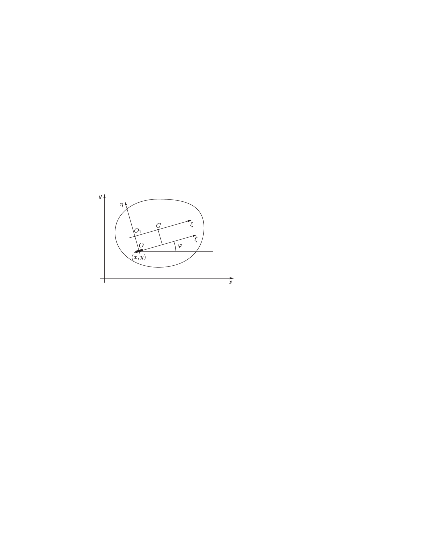
Fig. 2:

Without loss of generality, the rigid body itself may be assumed to be flat. The positions of this body on the plane are determined by three parameters: the Cartesian coordinates $x$ and $y$ of a distinguished point $O$, and the rotation angle $\varphi$ (Fig. 2). The independent left-invariant fields on $E(2)$ are specified by the differential operators

$$X_{\xi}=\cos\varphi\,\frac{\partial}{\partial x}+\sin\varphi\,\frac{\partial}{\partial y},\quad X_{\eta}=-\sin\varphi\,\frac{\partial}{\partial x}+\cos\varphi\,\frac{\partial}{\partial y},\quad X_{\varphi}=\frac{\partial}{\partial\varphi}.$$

The commutation relations (1) are

$$[X_{\xi},X_{\varphi}]=-X_{\eta},\quad[X_{\eta},X_{\varphi}]=X_{\xi},\quad[X_{\xi},X_{\eta}]=0.$$ (9)

Let $\xi$, $\eta$ be the coordinates of the center of mass of the body $G$ in a moving reference frame, $u$, $v$ be the projections of the velocity of the origin of the moving frame onto these axes, and $\omega$ be the angular velocity. The nonintegrable constraint equation is

$$f=v=0.$$ (10)

This constraint is left-invariant.

Let $m$ be the mass of the body and $J_{0}$ be its inertia moment relative to the center of mass. The kinetic energy

$$T=\frac{m}{2}\Big{(}(u-\omega\eta)^{2}+(v+\omega\xi)^{2}\Big{)}+\frac{J_{0}\omega^{2}}{2}$$ (11)

is also left-invariant: like the constraint function, it is independent of the generalized coordinates. Hence, the Chaplygin sleigh is an example of an EPS system on the group $E(2)$.

Taking into account (9), the EPS equations for the Chaplygin sleigh take the form

$$\bigg{(}\frac{\partial T}{\partial u}\bigg{)}^{\boldsymbol{\cdot}}=\omega\frac{\partial T}{\partial v},\quad\bigg{(}\frac{\partial T}{\partial v}\bigg{)}^{\boldsymbol{\cdot}}=-\omega\frac{\partial T}{\partial u}+\lambda,\quad\bigg{(}\frac{\partial T}{\partial\omega}\bigg{)}^{\boldsymbol{\cdot}}=v\frac{\partial T}{\partial u}-u\frac{\partial T}{\partial v}.$$ (12)

Of course, one needs to add to them the constraint equation (10).

The second equation serves as the basis for finding the Lagrange multiplier (the constraint reaction), and the first and the third equations (taking into account the constraint) have the following explicit form:

$$\dot{u}-\eta\dot{\omega}=\xi\omega^{2},\quad(J_{0}+m\xi^{2}+m\eta^{2})\dot{\omega}-m\eta\dot{u}=-m\xi u\omega.$$ (13)

These equations should be supplemented with those describing the law of motion of the point $O$ and the rotation angle $\varphi$:

$$\dot{x}=u\cos\varphi,\quad\dot{y}=u\sin\varphi,\quad\dot{\varphi}=\omega.$$ (14)

A qualitative analysis of motion of the Chaplygin sleigh for $\eta=0$ can be found in [24]. We supplement this analysis with some remarks.

Proposition 1.

​​[17]. If $\eta\neq 0$, then the equations of motion in the coordinate frame $O_{1}\xi\eta$ with the origin $O_{1}$ lying at the intersection of the straight line $O_{1}G$ which is parallel to the blade and passes through the center of mass, and the straight line $OO_{1}$ which is perpendicular to $O_{1}G$ and passes through the contact point of the blade, coincide with the equations of motion (13), (14) in the frame $O\xi\eta$ when $\eta=0$.

Thus, if we consider the trajectory of point $O_{1}$ instead of the trajectory of the contact point of the blade, then without loss of generality we may set $\eta=0$ in the equations of motion (13).

If $\xi=0$, all motions are steady. If $\xi\neq 0$, the phase portrait of the system (13) is similar in appearance to the phase portrait of Suslov’s problem (Fig. 1). In particular, the nonlinear equations (13) do not admit an invariant measure with a summable density. The steady–state solutions of (13)

$$u=u_{0},\quad\omega=0$$

correspond to the rectilinear motions of the Chaplygin sleigh. They are stable for $\xi u_{0}>0$ and unstable for $\xi u_{0}<0$. Thus, during a stable motion in a straight line, the center of mass of the body ‘‘outstrips’’ the contact point of the wheel. Here a change in stability occurs when the direction of motion is reversed.

In fact, the system’s global evolution on the time interval $t\in(-\infty,+\infty)$ in this case may be considered as a scattering process, that is, as $t\to-\infty$, the sleigh ‘‘starts’’ its motion from some unstable steady–state solution (the center of mass ‘‘lags behind’’ the contact point), undergoes some evolution, and tends to some stable steady-state solution as $t\to+\infty$. At the same time, the complete rotation angle of the axis $O\xi$ (or the axis $O\xi_{1}$) is independent of the initial conditions and, according to [17], is defined by

$$\Delta\varphi\big{|}_{-\infty}^{+\infty}=\pi A,\quad A^{2}=\bigg{(}1+\frac{J_{0}}{m\xi^{2}}\bigg{)}.$$

The Hamiltonian representation of the system (13)-(14) and the redundant set of first integrals are also given in [17].

Typical trajectories of point $O_{1}$ for various values of $A$ are shown in Fig. 3.

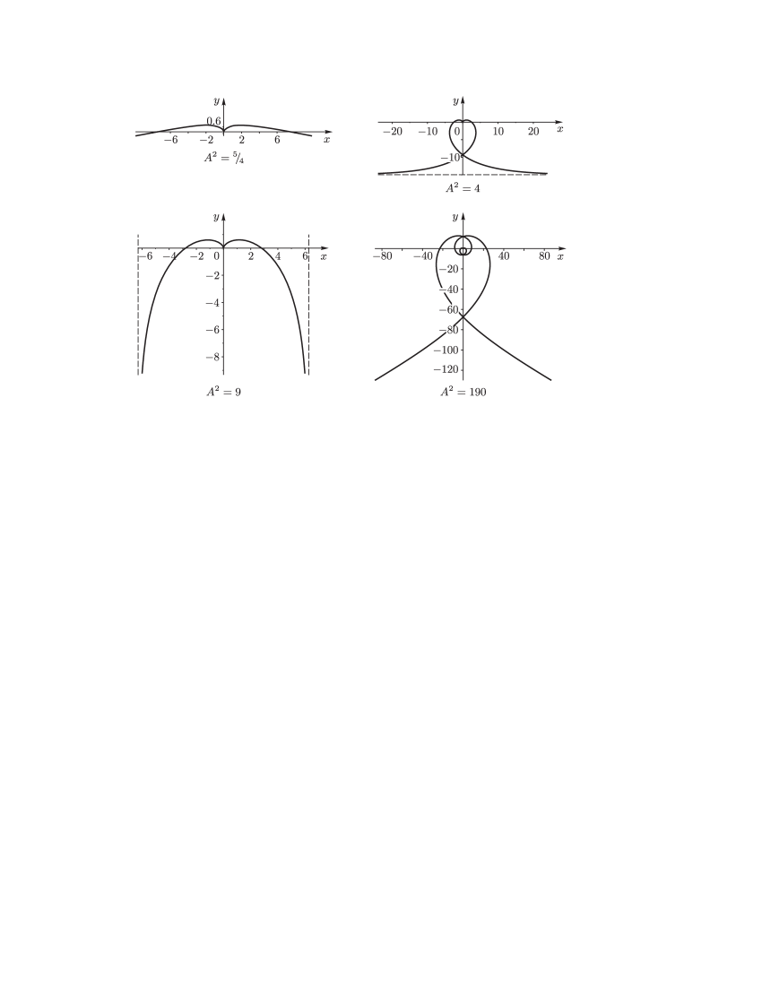
Fig. 3:

Examples of other nonholonomic systems represented in Hamiltonian and conformally Hamiltonian forms are given in [7, 5, 6, 3]. We also note that the motion of the Chaplygin sleigh on a rotating plane is considered in [31].

Remark 1.

There is a simple and natural connection between Suslov’s and Chaplygin’s problems. We consider the generalized Chaplygin sleigh on a two-dimensional sphere: this is a spherical ‘‘cap’’ sliding on the sphere with the nonholonomic constraint. Its dynamics are described by Suslov’s equations. In the extreme case, as the radius of the sphere increases to infinity, we obtain the Chaplygin sleigh. This technique includes the well-known retraction of the group $SO(3)$ to the group $E(3)$.

3 Anisotropic friction

A nonholonomic model describes the dynamics of systems with ideal constraints. There exist more realistic models which take into account large forces of viscous friction with anisotropic Rayleigh’s function, see, for example, [18]. Thecorresponding passage to the limit with regard to the Chaplygin sleigh was studied in [8, 24].

Following Carathéodory, we consider the motion of a rigid body ona horizontal plane taking into account the force of viscous friction applied to a fixed point of the rigid body and orthogonal to some body-fixed direction. In the notation of Section 2 the equations of motion are described by the following closed system on the algebra $e(3)$:

$$\bigg{(}\frac{\partial T}{\partial u}\bigg{)}^{\boldsymbol{\cdot}}=\omega\frac{\partial T}{\partial v},\quad\bigg{(}\frac{\partial T}{\partial v}\bigg{)}^{\boldsymbol{\cdot}}=-\omega\frac{\partial T}{\partial u}-kv,\quad\bigg{(}\frac{\partial T}{\partial\omega}\bigg{)}^{\boldsymbol{\cdot}}=v\frac{\partial T}{\partial u}-u\frac{\partial T}{\partial v}.$$ (15)

Here, $k>0$ is the coefficient of viscous friction. In contrast to (12), there are no constraints here. We write the explicit form of these nonlinear equations:

$$\begin{gathered}\dot{u}-\eta\dot{\omega}=\omega v+\xi\omega^{2},\quad\dot{v}+\xi\dot{\omega}=-\omega u+\eta\omega^{2}-\frac{k}{m}\,v,\\ \frac{J}{m}\,\dot{\omega}+\xi\dot{v}-\eta\dot{u}=-\omega(\xi u+\eta v).\end{gathered}$$ (16)

Here, $J=J_{0}+m(\xi^{2}+\eta^{2})$ is the moment of inertia of the body about the distinguished point.

Like (12), the system (16) has the family of steady-state solutions

$$u=u_{0},\quad v=0,\quad\omega=0$$ (17)

corresponding to the motion of a rigid body in a straight line with a constant velocity. In view of the equality $\dot{T}=-kv^{2}$, the energy does not dissipate on these solutions. In order to study the stability of the solutions (17), we linearize in their neighborhood Eqs.  (16). Omitting simple calculations, we give the characteristic polynomial of the linearized system:

$$f(\lambda)=\lambda\bigg{[}\lambda^{2}\frac{J_{0}}{m}+\lambda\frac{J_{0}+m\xi^{2}}{m^{2}}+\frac{\xi u_{0}k}{m}\bigg{]}.$$ (18)

The appearance of the zero root is due to the fact that the steady-state solutions (17) are nonisolated.

If $\xi u_{0}<0$ (the contact point ‘‘outstrips’’ the center of mass when the body is moving), the characteristic polynomial has a real positive root and therefore the steady motion in a straight line is unstable (as in the case of the Chaplygin sleigh).

We show that given $\xi u_{0}>0$ (when the center of mass ‘‘outstrips’’ the contact point) the steady motion is stable. Moreover, perturbed motions asymptotically tend to one of the steady states (17). By Lyapunov’s classical theorem [22, Section 32], it is sufficient to show that the nonzero roots of the characteristic polynomial (18) have negative real parts. But this, in turn, follows from the positivity property of the coefficients of the polynomial (18).

We also present the asymptotic form of the roots of the characteristicpolynomial as $k\,{\to}\,\infty$:

$$\lambda_{1}=0,\quad\lambda_{2}=-\frac{m\xi u_{0}}{J_{0}+m\xi^{2}}+O\bigg{(}\frac{1}{k}\bigg{)},\quad\lambda_{3}=-\frac{J_{0}+m\xi^{2}}{J_{0}m}\,k+O(1).$$

It is clear that $\lambda_{3}\to-\infty$ as $k\to\infty$, and

$$\lambda_{2}\to-\frac{m\xi u_{0}}{J_{0}+m\xi^{2}}.$$ (19)

The unbounded decrease in one of the eigenvalues corresponds to the limit passage to the nonholonomic dynamics of the Chaplygin sleigh (taking into account the boundary layer phenomenon [8, 24]). The limit relation (19) gives a formula for the eigenvalue of steady-state solutions of the nonholonomicequations (13).

4 The general case

These observations can be generalized. Eqs. (4) are a closed system of ${n-m}=p\geq 2$ differential equations with quadratic right-hand sides. Indeed, quasi-velocities can be chosen in such a way that the linear functions of constraints take the form: $f_{1}=\omega_{n-m+1},\ldots,f_{m}=\omega_{n}$. Then the first $n-m$ equations of (4) form a closed system with the quadratic right-hand side

$$\dot{\omega}=v(\omega),\quad\omega=\left(\omega_{1},\ldots,\omega_{n-m}\right)^{\top}\in\mathbb{R}^{p},$$ (20)

and Lagrange multipliers can be found from the remaining $m$ equations. The system (20) admits the first integral $H$ as a positive definite quadratic form.

The problem of finding nonzero steady-state solutions $\omega_{0}$ to the nonlinear system (20) is a nontrivial algebraic problem. It depends on the structure constants of the algebra $g$, the inertia tensor, and the linear functions ofconstraints. The homogeneity of the system (20)

$$v(\lambda\omega)=\lambda^{2}v(\omega),\quad\lambda\in\mathbb{R},$$ (21)

implies the following simple property: if $\omega=\omega_{0}$ is a steady-state solution, then the whole straight line

$$\omega=\mu\omega_{0},\quad\mu\in\mathbb{R},$$ (22)

consists of steady-state solutions. We call the straight line (22) a straight line of steady motions (which we abbreviate as SLSM).

The general number of nonzero nonproportional solutions of the algebraic system of equations

$$v_{1}(\omega)=0,\ldots,v_{p}(\omega)=0$$ (23)

(including the complex solutions) can be estimated using the Bezout theorem: if the number of these solutions is finite, it does not exceed $2^{p-1}$. Indeed, from the algebraic system (23) we select $p-1$ equations so that the number of their nonproportional solutions (with the complex ones) is finite. Since the number of variables equals $p$ and all functions $v_{1},\ldots,v_{p}$ are homogeneous in $\omega$ with homogeneity degree $2$, then (by the Bezout theorem) the number of solutions (with multiplicities taken into account) equals $2^{p-1}$. All these solutions should satisfy one more (omitted) equation. Therefore, their general number obviously does not increase.

This estimate is rough and does not take into account the existence of the positive definite quadratic integral of the system (20).

Theorem 1.

If $p=2$, then either all positions are steady ($v_{1}=v_{2}\equiv 0$) or there is only one SLSM.

Thus, if $p=2$, the phase portrait of the system (20) is similar in appearance to the phase portraits in Suslov’s and Chaplygin’s problems. Theorem 1 shows universality of stability changes in EPS systems with two nonholonomic degrees of freedom when the direction of motion is reversed. Theorem 1 also shows that the general estimate of the number of SLSMs based on the Bezout theorem is not accurate.

Proof.

of Theorem 1. By a linear change of independent variables the first integral of the system (20) is reduced to the form

$$H=\frac{1}{2}\left(\omega^{2}_{1}+\omega^{2}_{2}\right)\!.$$

In these variables, let

$$v_{i}=a_{i}\omega^{2}_{1}+b_{i}\omega_{1}\omega_{2}+c_{i}\omega^{2}_{2},\quad i=1,2.$$

The condition $\dot{H}=0$ gives the following relations for the coefficients: $a_{1}=c_{2}=0$, $b_{1}=-a_{2}$, $c_{1}=-b_{2}$. Hence, Eqs. (20) become

$$\dot{\omega}_{1}=\omega_{2}(b_{1}\omega_{1}+c_{1}\omega_{2}),\quad\dot{\omega}_{2}=-\omega_{1}(b_{1}\omega_{1}+c_{1}\omega_{2}).$$ (24)

If $b_{1}=c_{1}=0$, then $v_{1}=v_{2}\equiv 0$. But if $b^{2}_{1}+c^{2}_{1}\neq 0$, there is only one SLSM: $b_{1}\omega_{1}+c_{1}\omega_{2}=0$. QED.

Eqs. (24) can be given the conformally Hamiltonian form

$$\dot{\omega_{1}}=\rho\frac{\partial H}{\partial\omega_{2}},\quad\dot{\omega_{2}}=-\rho\frac{\partial H}{\partial\omega_{1}};\quad\rho=b_{1}\omega_{1}+c_{1}\omega_{2}.$$

They take the canonical form after rescaling time as $d\tau=\rho\,dt$. The multiplier $\rho^{-1}$ serves as the density of the integral invariant of the system (20). However, this function has singularities on the SLSM and reverses sign when crossing this straight line. Conformally Hamiltonian systems naturally arise in problems of nonholonomic mechanics [26, 3].

Let $\omega=\omega_{0}$ be a steady motion. Set

$$A=\left.\frac{\partial v}{\partial\omega}\right|_{\omega_{0}}.$$ (25)

This is the linearization operator of the system (20) at point $\omega_{0}$. Differentiating the identity (21) with respect to $\lambda$ and then assuming that $\lambda=1$, we obtain

$$\frac{\partial v}{\partial\omega}\,\omega=2v(\omega).$$

If $\omega=\omega_{0}$, we have $A\omega_{0}=0$. Therefore, the operator (25) is degenerate. By $u(\omega_{0})$ ($s(\omega_{0})$) we denote the number of eigenvalues of the operator (25) lying in the right (respectively, left) complex half-plane. The following simple theorem holds:

Theorem 2.

If $\omega_{0}\neq 0$ is a steady motion, then for $\mu>0$

$$u(\mu\omega_{0})=u(\omega_{0}),\quad s(\mu\omega_{0})=s(\omega_{0}),$$

and for $\mu<0$

$$u(\mu\omega_{0})=s(\omega_{0}),\quad s(\mu\omega_{0})=u(\omega_{0}).$$

Indeed, according to (25), the eigenvalues of the linearization operator of at the stationary point $\mu\omega_{0}$ differ from those of the operator $A$ by the multiplier $\mu$.

In the case that is the most important to us

$$s(\omega_{0})=n-m-1.$$

Then (with the zero root) $u(\omega_{0})=0$ and, by Lyapunov’s theorem, the equilibrium point $\omega_{0}$ is stable. Moreover, the perturbed motion infinitely approaches one of the equilibria (22) as $t\to+\infty$. On the other hand, by Theorem 2, $u(-\omega_{0})$ also equals $n-m-1>0$. Therefore, the steady motion $\omega=-\omega_{0}$ is unstable.

We call the SLSM (22) nondegenerate if at all points of this straight line, ${\omega\neq 0}$, the operator (25) has only one zero eigenvalue. We define the index of the nondegenerate SLSM:

$$i=j(\omega_{0})+j(-\omega_{0}),\quad\omega_{0}\neq 0,$$ (26)

where $j(\omega_{0})=1$ ($=-1$) if $s(\omega_{0})$ is even (odd). By Theorem 2, the index is independent of the choice of point $\omega_{0}\neq 0$ on the straight line (22). The index can take the following values: $-2$, $0$, $2$. If $p$ is even, then (by Theorem 2) $i=0$.

Theorem 3.

If all SLSMs are nondegenerate, then the sum of their indices equals $1+(-1)^{p+1}$.

In order to prove it, we fix the positive level set of the energy integral ${H=h>0}$ and restrict the initial dynamical system (20) to it. It is only the equilibrium points of the reduced system on the $(p-1)$-dimensional ellipsoid $\{H(\omega)=h\}$ that coincide with the points of intersection of the SLSM (22) with this ellipsoid. In view of the assumption about nondegeneracy of the SLSM, all equilibria of the reduced system are isolated. The index of the singular point $\omega_{0}$ of the system on the energy ellipsoid is defined as the sign of product of the roots of the characteristic polynomial of the linearization operator for the reduced system at point $\omega_{0}$. It is clear that these numbers coincide with the eigenvalues of the operator (25) other than zero. Their product sign obviously coincides with the number $j(\omega_{0})$ from (26). It remains to use the Poincaré–Hopf theorem: the sum of the indices of isolated singular points of a dynamical system on a closed manifold is equal to its Eulerian characteristic. Recall that the Eulerian characteristic of the $(p-1)$-dimensional sphere is equal to zero for even $p$ and is equal to $2$ for odd $p$. QED.

Corollary 1.

If $p$ is odd, then there is at least one SLSM.

Corollary 2.

If $p$ is odd and all SLSMs are nondegenerate, then their number is odd. In particular, it does not exceed $2^{p-1}-1$.

Indeed, for odd $p$ the index of the SLSM can be either $-2$ or $2$. If the number of nondegenerate SLSMs is even, then the sum of the indices is divisible by $4$. However, (by Theorem 3) this sum equals $2$. Further, by the Bezout theorem, there are at most $2^{p-1}$ nondegenerate SLSMs. But for $p\geq 2$ this is an even number. Hence, the total number of SLSMs does not exceed $2^{p-1}-1$.

It is not improbable that the conclusions of Corollaries 1 and 2 hold for even values of $p$, too. In any case, this holds for $p=2$ (Theorem 1). When $p=3$, there is either one or three nondegenerate SLSMs. The latter case takes place for the Euler top when the inertia moments are unequal.

In conclusion, we mention that a nonholonomic system of two coupled bodies (called a nonholonomic hinge and generalizing the Suslov problem) is considered in [32]. Evidently, the above methods can be applied to this problem as well.

References

- [1] Arnold V. I., Sur la géométrie différentielle des groups de Lie de dimension infinite et ses applications à l’hydrodynamique des fluides parfaits, Ann. Inst. Fourier, 1966, vol. 16, no. 1, pp. 319–361.
- [2] Bolsinov A. V., Borisov A. V. and Mamaev I. S., Hamiltonization of Nonholonomic Systems in the Neighborhood of Invariant Manifolds, Regul. Chaotic Dyn., 2011, vol. 16, no. 5, pp. 443–464.
- [3] Borisov A. V., Fedorov Yu. N. and Mamaev I. S., Chaplygin Ball over a Fixed Sphere: An Explicit Integration, Regul. Chaotic Dyn., 2008, vol. 13, no. 6, pp. 557–571.
- [4] Borisov A. V., Jalnine A. Yu., Kuznetsov S. P., Sataev I. R. and Sedova J. V., Dynamical Phenomena Occurring due to Phase Volume Compression in Nonholonomic Model of the Rattleback, Regul. Chaotic Dyn., 2012, vol. 17, no. 6, pp. 512–532.
- [5] Borisov A. V. and Mamaev I. S., The Rolling Motion of a Rigid Body on a Plane and a Sphere: Hierarchy of Dynamics, Regul. Chaotic Dyn., 2002, vol. 7, no. 2, pp. 177–200.
- [6] Borisov A. V. and Mamaev I. S., Rolling of a Non-Homogeneous Ball over a Sphere without Slipping and Twisting, Regul. Chaotic Dyn., 2007, vol. 12, no. 2, pp. 153–159.
- [7] Borisov A. V. and Mamaev I. S., Conservation Laws, Hierarchy of Dynamics and Explicit Integration of Nonholonomic Systems, Regul. Chaotic Dyn., 2008, vol. 13, no. 5, pp. 443–490.
- [8] Caratheodory C., Der Schlitten, Z. Angew. Math. Mech., 1933, vol. 13, pp. 71–76.
- [9] Fedorov Yu. N., Maciejewski A. J. and Przybylska M., Suslov Problem: Integrability, Meromorphic and Hypergeometric Solutions, Nonlinearity, 2009, vol. 22, no. 9, pp. 2231–2259.
- [10] Jovanović B., Some Multidimensional Integrable Cases of Nonholonomic Rigid Body Dynamics, Regul. Chaotic Dyn., 2003, vol. 8, no. 1, pp. 125–132.
- [11] Kozlov V. V. and Fedorov Yu. N., Various Aspects of -Dimensional Rigid Body Dynamics, in Dynamical Systems in Classical Mechanics, Amer. Math. Soc. Transl. Ser. 2, vol. 168, Providence, R.I.: AMS, 1995, pp. 141–171.
- [12] Poincaré H., Sur une forme nouvelle des équations de la Mécanique, C. R. Acad. Sci., 1901, vol. 132, pp. 369–371.
- [13] Walker G. T., On a Dynamical Top, Quart. J. Pure Appl. Math., 1896, vol. 28, pp. 174–185.
- [14] Zenkov D. V. and Bloch A. M., Dynamics of the -Dimensional Suslov Problem, J. Geom. Phys., 2000, vol. 34, no. 2, pp. 121–136.
- [15] Borisov A. V., Kilin A. A. and Mamaev I. S., Hamiltonian Representation and Integrability of the Suslov Problem, Nelin. Dinam., 2010, vol. 6, no. 1, pp. 127–142 (Russian).
- [16] Borisov A. V. and Mamaev I. S., Strange Attractors in Rattleback Dynamics, Physics Uspekhi, 2003, vol. 46, no. 4, pp. 393–403; see also: Uspekhi Fiz. Nauk, 2003, vol. 173, no. 4, pp. 407–418.
- [17] Borisov A. V. and Mamaev I. S., The Dynamics of a Chaplygin Sleigh, J. Appl. Math. Mech., 2009, vol. 73, no. 2, pp. 156–161; see also: Prikl. Mat. Mekh., 2009, vol. 73, no. 2, pp. 219–225.
- [18] Kozlov V. V., Realization of Nonintegrable Constraints in Classical Mechanics, Sov. Phys. Dokl., 1983, vol. 28, pp. 735–737; see also: Dokl. Akad. Nauk SSSR, 1983, vol. 272, no. 3, pp. 550–554.
- [19] Kozlov V. V., On the Theory of Integration of the Equations of Nonholonomic Mechanics, Uspekhi Mekh., 1985, vol. 8, no. 3, pp. 85–107 (Russian).
- [20] Kozlov V. V., Invariant Measures of Euler – Poincaré Equations on Lie Algebras, Funct. Anal. Appl., 1988, vol. 22, no. 1, pp. 58–59; see also: Funktsional. Anal. i Prilozhen., 1988, vol. 22, no. 1, pp. 69–70.
- [21] Kozlov V. V., The Euler – Jacobi – Lie Integrability Theorem, Regul. Chaotic Dyn., 2013, vol. 18, no. 4, pp. 329–343.
- [22] Lyapunov A. M., The General Problem of the Stability of Motion, Moscow: Gostekhizdat, 1950 (Russian).
- [23] Markeev A. P., Dynamics of a Body Touching a Rigid Surface, Moscow–Izhevsk: R&C Dynamics, Institute of Computer Science, 2014 (Russian).
- [24] Neimark Ju. I. and Fufaev N. A., Dynamics of Nonholonomic Systems, Trans. Math. Monogr., vol. 33, Providence, RI: AMS, 1972.
- [25] Suslov G. K., Theoretical Mechanics, Moscow: Gostekhizdat, 1946 (Russian).
- [26] Chaplygin S. A., On the Theory of Motion of Nonholonomic Systems. The Reducing-Multiplier Theorem, Regul. Chaotic Dyn., 2008, vol. 13, no. 4, pp. 369–376; see also: Mat. Sb., 1912, vol. 28, no. 2, pp. 303–314.
- [27] Fedorov Yu. N., Maciejewski A. J. and Przybylska M., The Poisson equations in the nonholonomic Suslov problem: integrability, meromorphic and hypergeometric solutions, Nonlinearity, 2009, vol. 22, pp. 2231–2259.
- [28] Borisov A. V., Kazakov A. O. and Sataev I. R., The reversal and chaotic attractor in the nonholonomic model of Chaplygin s top, Regul. Chaotic Dyn., 2014, vol. 19, no. 6, pp. 718–733.
- [29] Gonchenko A. S., Gonchenko S. V. and Kazakov A. O., Richness of chaotic dynamics in nonholonomic models of a Celtic stone, Regul. Chaotic Dyn., 2013, vol. 18, no. 5, pp. 521–538.
- [30] Borisov A. V., Mamaev I. S. and Bizyaev I. A., The hierarchy of dynamics of a rigid body rolling without slipping and spinning on a plane and a sphere, Regul. Chaotic Dyn., 2013, vol. 18, no. 3, pp. 277–328.
- [31] Borisov A. V., Mamaev I. S. and Bizyaev I. A., The Jacobi integral in nonholonomic mechanics, Regul. Chaotic Dyn., 2015, vol. 20, no. 3, pp. 383–400.
- [32] Bizyaev I. A., Borisov A. V. and Mamaev I. S. The dynamics of nonholonomic systems consisting of a spherical shell with a moving rigid body inside, Regul. Chaotic Dyn., 2014, vol. 19, no. 2, pp. 198–213.