Nonclassical readout of optical memories under local energy constraint

Abstract

Nonclassical states of light play a central role in many quantum information protocols. Very recently, their quantum features have been exploited to improve the readout of information from digital memories, modeled as arrays of microscopic beam splitters [S. Pirandola, Phys. Rev. Lett. 106, 090504 (2011)]. In this model of “quantum reading”, a nonclassical source of light with Einstein-Podolski-Rosen correlations has been proven to retrieve more information than any classical source. In particular, the quantum-classical comparison has been performed under a global energy constraint, i.e., by fixing the mean total number of photons irradiated over each memory cell. In this paper we provide an alternative analysis which is based on a local energy constraint, meaning that we fix the mean number of photons per signal mode irradiated over the memory cell. Under this assumption, we investigate the critical number of signal modes after which a nonclassical source of light is able to beat any classical source irradiating the same number of signals.

1 Introduction

Quantum information has disclosed a modern approach to both quantum mechanics and information theory [1]. Very recently, this field has been developed into the so-called “continuous variable” setting, where information is encoded and processed using quantum systems with infinite dimensional Hilbert spaces [2, 3, 4, 5, 6]. Bosonic systems, such as the radiation modes of the electromagnetic field, are today the most studied continuous variable systems, thanks to their strict connection with quantum optics. In the continuous variable framework, a wide range of results have been successfully achieved, including quantum teleportation [7, 8, 9, 10, 11, 12], teleportation networks [13, 14, 15] and games [16, 17], entanglement swapping protocols [18, 19, 20], quantum key distribution [21, 22, 23, 24, 25], two-way quantum cryptography [26, 27], quantum computation [28, 29, 30, 31, 32, 33, 34] and cluster quantum computation [35, 36, 37, 38]. Other studies have lead to the full classification of Gaussian channels and collective Gaussian attacks [39, 40, 41], the computation of secret-key capacities and their reverse counterpart [42, 43, 44, 45, 46], and possible schemes for quantum direct communication [47, 48].

One of the key resources in many protocols of quantum information is quantum entanglement. In the bosonic setting, quantum entanglement is usually present under the form of Einstein-Podolski-Rosen (EPR) correlations [49], where the quadrature operators of two separate bosonic modes are so correlated to beat the standard quantum limit [50]. The simplest source of EPR correlations is the two-mode squeezed vacuum (TMSV) state. In the number-ket representation this state is defined by

$$\left|\xi\right\rangle=(\cosh\xi)^{-1}\sum_{n=0}^{\infty}(\tanh\xi)^{n}\left|n\right\rangle_{s}\left|n\right\rangle_{i}~{},$$

where $\xi$ is the squeezing parameter and $\{s,i\}$ is an arbitrary pair of bosonic modes, that we may call “signal” and “idler”. In particular, $\xi$ quantifies the signal-idler entanglement and gives the mean number of photons sinh${}^{2}\xi$ in each mode. Since it is entangled, the TMSV state cannot be prepared by applying local operations and classical communications (LOCCs) to a couple of vacua $\left|0\right\rangle_{s}\otimes\left|0\right\rangle_{i}$ or any other kind of tensor product state. For this reason, the TMSV state cannot be expressed as a classical mixture of coherent states $\left|\alpha\right\rangle_{s}\otimes\left|\beta\right\rangle_{i}$ with $\alpha$ and $\beta$ arbitrary complex amplitudes. In other words, its P-representation [58, 59]

$$\left|\xi\right\rangle\left\langle\xi\right|=\int\int d^{2}\alpha d^{2}\beta\boldsymbol{~{}}\mathcal{P}(\alpha,\beta)~{}\left|\alpha\right\rangle_{s}\left\langle\alpha\right|\otimes\left|\beta\right\rangle_{i}\left\langle\beta\right|~{},$$

involves a function $\mathcal{P}$ which is non-positive and, therefore, cannot be considered as a genuine probability distribution. For this reason, the TMSV state is a particular kind of “nonclassical” state. Other kinds are single-mode squeezed states and Fock states. By contrast a bosonic state is called “classical” when its P-representation is positive, meaning that the state can be written as a classical mixture of coherent states. Thus a classical source of light is composed by a set of $m$ bosonic modes in a state

$$\rho=\int d^{2}\alpha_{1}\cdots\int d^{2}\alpha_{m}\boldsymbol{~{}}\mathcal{P}(\alpha_{1},\cdots,\alpha_{m})~{}\otimes_{k=1}^{m}\left|\alpha_{k}\right\rangle\left\langle\alpha_{k}\right|~{},$$ (1)

where $\mathcal{P}$ is positive and normalized to $1$. Typically, classical sources are just made by collection of coherent states with amplitudes $\{\bar{\alpha}_{1},\cdots,\bar{\alpha}_{m}\}$, i.e., $\rho=\otimes_{k=1}^{m}\left|\bar{\alpha}_{k}\right\rangle\left\langle\bar{\alpha}_{k}\right|$ which corresponds to have

$$\mathcal{P}=\prod_{k=1}^{m}\delta^{2}(\alpha_{k}-\bar{\alpha}_{k})~{}.$$

In other situations, where the sources are particularly chaotic, they are better described by a collection of thermal states with mean photon numbers $\{\bar{n}_{1},\cdots,\bar{n}_{m}\}$, so that

$$\mathcal{P}=\prod_{k=1}^{m}\frac{\exp(-\left|\alpha_{k}\right|^{2}\bar{n}_{k})}{\pi\bar{n}_{k}}~{}.$$

More generally, we can have classical states which are not just tensor products but they have (classical) correlations among different bosonic modes.

The comparison between classical and nonclassical states has clearly triggered a lot of interest. The main idea is to compare the use of a candidate nonclassical state, like the EPR state, with all the classical states for specific information tasks. One of these tasks has been the detection of low-reflectivity objects in far target regions under the condition of extremely low signal-to-noise ratios. This scenario has been called “quantum illumination” and has been investigated in a series of papers [51, 52, 53, 54, 55, 56].

Most recently, the EPR correlations have been exploited for a completely different task in a completely different regime of parameters. In the model of “quantum reading” [57], the EPR correlations have been used to retrieve information from digital memories which are reminiscent of today’s optical disks, such as CDs and DVDs. A digital memory can in fact be modelled as a sequence of cells corresponding to beam splitters with two possible reflectivities $r_{0}$ and $r_{1}$ (used to encode a bit of information). By fixing the mean total number of photons $N$ irradiated over each memory cell, it is possible to show that a non-classical source of light with EPR correlations retrieves more information than any classical source [57]. In general, the improvement is found in the regime of few photons ($N=1\div 100$) and for memories with high reflectivities, as typical for optical memories. In this regime, the gain of information given by the quantum reading can be dramatic, i.e., close to $1$ bit for each bit of the memory.

An important point in the study of Ref. [57] is that the quantum-classical comparison is performed under a global energy constraint, i.e., by fixing the total number of photons $N$ which are irradiated over each memory cell (on average). Under this assumption, it is possible to construct an EPR transmitter, made by a suitable number of TMSV states, which is able to outperform any classical source composed by any number of modes. In the following we consider a different and easier comparison: we fix the number of signal modes irradiated over the target cell ($M$) and the mean number of photons per signal mode ($N_{S}$). Under these assumptions, we compare an EPR transmitter with a classical source. Then, for fixed $N_{S}$, we determine the critical number of signal modes $M^{(N_{S})}$ after which an EPR transmitter with $M>$ $M^{(N_{S})}$ is able to beat any classical source (with the same number of signals $M$).

2 Readout mechanism

Here we briefly review the basic readout mechanism of Ref. [57], specifying the study to the case of a local energy constraint. Let us consider a model of digital optical memory (or disk) where the memory cells are beam splitter mirrors with different reflectivities $r=r_{0},r_{1}$ (with $r_{1}\geq r_{0}$). In particular, the bit-value $u=0$ is encoded in a lower-reflectivity mirror ($r=r_{0}$), that we may call a pit, while the bit-value $u=1$ is encoded in a higher-reflectivity mirror ($r=r_{1}$), that we may call a land (see Fig. 1). Close to the disk, a reader aims to retrieve the value of the bit $u$ which is stored in each memory cell. For this sake, the reader exploits a transmitter (to probe a target cell) and a receiver (to measure the corresponding output). In general, the transmitter consists of two quantum systems, called signal $S$ and idler $I$, respectively. The signal system $S$ is a set of $M$ bosonic modes which are directly shined on the target cell. The mean total number of photons of this system is simply given by $N=MN_{S}$, where $N_{S}$ is the mean number of photons per signal mode (simply called “energy”, hereinbelow). At the output of the cell, the reflected system $R$ is combined with the idler system $I$, which is a supplementary set of bosonic modes whose number $L$ can be completely arbitrary. Both the systems $R$ and $I$ are finally measured by the receiver (see Fig. 1).

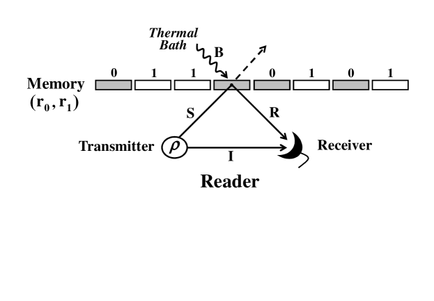
Figure 1: Model of memory. Digital information is stored in a disk whose memory cells are beam splitter mirrors with different reflectivities: $r=r_{0}$ encoding bit-value $u=0$ and $r=r_{1}$ encoding bit-value $u=1$. Readout. A reader is generally composed by a transmitter and a receiver. It retrieves a stored bit by probing a memory cell with a signal system $S$ ($M$ bosonic modes) and detecting the reflected system $R$ together with an idler system $I$ ($L$ bosonic modes). In general, the output system $R$ combines the signal system $S$ with a bath system $B$ ($M$ bosonic modes in thermal states). The transmitter is in a state $\rho$ which can be classical (classical transmitter) or non-classical (quantum transmitter). In our work, we consider a quantum transmitter with EPR correlations between signal and idler systems.

We assume that Alice’s apparatus is very close to the disk, so that no significant source of noise is present in the gap between the disk and the decoder. However, we assume that non-negligible noise comes from the thermal bath present at the other side of the disk. This bath generally describes stray photons, transmitted by previous cells and bouncing back to hit the next ones. For this reason, the reflected system $R$ combines the signal system $S$ with a bath system $B$ of $M$ modes. These environmental modes are assumed in a tensor product of thermal states, each one with $N_{B}$ mean photons (white thermal noise). In this model we identify five basic parameters: the reflectivities of the memory $\{r_{0},r_{1}\}$, the temperature of the bath $N_{B}$, and the profile of the signal $\{M,N_{S}\}$, which is given by the number of signals $M$ and the energy $N_{S}$.

In general, for a fixed input state $\rho$ at the transmitter (systems $S,I$), Alice will get two possible output states $\sigma_{0}$ and $\sigma_{1}$ at the receiver (systems $R,I$). These output states are the effect of two different quantum channels, $\mathcal{E}_{0}$ and $\mathcal{E}_{1}$, which depend on the bit $u=0,1$ stored in the target cell. In particular, we have $\sigma_{u}=(\mathcal{E}_{u}\otimes\mathcal{I})(\rho)$, where the conditional channel $\mathcal{E}_{u}$ acts on the signal system, while the identity channel $\mathcal{I}$ acts on the idler system. More exactly, we have $\mathcal{E}_{u}=\mathcal{R}_{u}^{\otimes M}$, where $\mathcal{R}_{u}$ is a one-mode lossy channel with conditional loss $r_{u}$ and fixed thermal noise $N_{B}$. Now, the minimum error probability $P_{err}$ affecting the decoding of $u$ is just the error probability affecting the statistical discrimination of the two output states, $\sigma_{0}$ and $\sigma_{1}$, via an optimal receiver. This quantity is equal to $P_{err}=[1-D(\sigma_{0},\sigma_{1})]/2$, where $D(\sigma_{0},\sigma_{1})$ is the trace distance between $\sigma_{0}$ and $\sigma_{1}$ [60, 61, 62]. Clearly, the value of $P_{err}$ determines the average amount of information which is decoded for each bit stored in the memory. This quantity is equal to $J=1-H(P_{err})$, where $H(x):=-x\log_{2}x-(1-x)\log_{2}(1-x)$ is the usual formula for the binary Shannon entropy. In the following, we compare the performance of decoding in two paradigmatic situations, one where the transmitter is described by a non-classical state (quantum transmitter) and one where the transmitter is in a classical state (classical transmitter). In particular, we show how a quantum transmitter with EPR correlations (EPR transmitter) is able to outperform classical transmitters. The quantum-classical comparison is performed for fixed signal profile $\{M,N_{S}\}$. Then, for various fixed values of the energy $N_{S}$ (local energy constraint), we study the critical number of signal modes $M^{(N_{S})}$ after which an EPR transmitter (with $M>M^{(N_{S})}$ signals) is able to beat any classical transmitter (with the same number of signals $M$).

3 Quantum-classical comparison

First let us consider a classical transmitter. A classical transmitter with $M$ signals and $L$ idlers is described by a classical state $\rho$ as specified by Eq. (1) with $m=M+L$. In other words it is a probabilistic mixture of multi-mode coherent states $\otimes_{k=1}^{M+L}\left|\alpha_{k}\right\rangle\left\langle\alpha_{k}\right|$. Given this transmitter, we consider the corresponding error probability $P_{err}^{class}$ which affects the readout of the memory. Remarkably, this error probability is lower-bounded by a quantity which depends on the signal profile $\{M,N_{S}\}$, but not from the number $L$ of the idlers and the explicit expression of the $\mathcal{P}$-function. In fact, we have [57]

$$P_{err}^{class}\geq\mathcal{C}(M,N_{S}):=\frac{1-\sqrt{1-F(N_{S})^{M}}}{2}~{},$$ (2)

where $F(N_{S})$ is the fidelity between $\mathcal{R}_{0}(|N_{S}^{1/2}\rangle\langle N_{S}^{1/2}|)$ and $\mathcal{R}_{1}(|N_{S}^{1/2}\rangle\langle N_{S}^{1/2}|)$, the two possible outputs of the single-mode coherent state $|N_{S}^{1/2}\rangle\langle N_{S}^{1/2}|$. As a consequence, all the classical transmitters with signal profile $\{M,N_{S}\}$ retrieve an information which is upper-bounded by $J_{class}:=1-H[\mathcal{C}(M,N_{S})]$.

Now, let us construct a transmitter having the same signal profile $\{M,N_{S}\}$, but possessing EPR correlations between signals and idlers. This is realized by taking $M$ identical copies of a TMSV state, i.e., $\rho=\left|\xi\right\rangle\left\langle\xi\right|^{\otimes M}$ where $N_{S}=\mathrm{sinh}^{2}\xi$. Given this transmitter, we consider the corresponding error probability $P_{err}^{quant}$ affecting the readout of the memory. This quantity is upper-bounded by the quantum Chernoff bound [63, 64, 65, 66, 67]

$$P_{err}^{quant}\leq\mathcal{Q}(M,N_{S}):=\frac{1}{2}\left[\inf_{s\in(0,1)}\mathrm{Tr}(\theta_{0}^{s}\theta_{1}^{1-s})\right]^{M},$$ (3)

where $\theta_{u}:=(\mathcal{R}_{u}\otimes\mathcal{I})(\left|\xi\right\rangle\left\langle\xi\right|)$. Since $\theta_{0}$ and $\theta_{1}$ are Gaussian states, we can write their symplectic decompositions [68] and compute the quantum Chernoff bound using the general formula for multimode Gaussian states given in Ref. [67]. Then, we can easily compute a lower bound $J_{quant}:=1-H[\mathcal{Q}(M,N_{S})]$ for the information which is decoded via this quantum transmitter.

In order to show an improvement with respect to the classical case, it is sufficient to prove the positivity of the “information gain” $G:=J_{quant}-J_{class}$. This quantity is in fact a lower bound for the average information which is gained by using the EPR quantum transmitter instead of every classical transmitter. Roughly speaking, the value of $G$ estimates the minimum information which is gained by the quantum readout for each bit of the memory. In general, $G$ is a function of all the basic parameters of the model, i.e., $G=G(M,N_{S},r_{0},r_{1},N_{B})$. Numerically, we can easily find signal profiles $\{M,N_{S}\}$, classical memories $\{r_{0},r_{1}\}$, and thermal baths $N_{B}$, for which we have the quantum effect $G>0$. Some of these values are reported in the following table.

$$~{}M~{}$$ bits

        

Note that we can find choices of parameters where $G\simeq 1$, i.e., the classical readout of the memory does not decode any information whereas the quantum readout is able to retrieve all of it. As shown in the last row of the table, this situation can occur when the both the reflectivities of the memory are very close to $1$. From the first row of the table, we can acknowledge another remarkable fact: for a land-reflectivity $r_{1}$ sufficiently close to $1$, one signal with few photons can give a positive gain. In other words, the use of a single, but sufficiently entangled, TMSV state $\left|\xi\right\rangle\left\langle\xi\right|$ can outperform every classical transmitter, which uses one signal mode with the same energy (and potentially infinite idler modes).

According to our numerical investigation, the quantum readout is generally more powerful when the land-reflectivity is sufficiently high (i.e., $r_{1}\gtrsim 0.8$). For this reason, it is very important to analyze the scenario in the limit of ideal land-reflectivity ($r_{1}=1$). Let us call “ideal memory” a classical memory with $r_{1}=1$. Clearly, this memory is completely characterized by the value of its pit-reflectivity $r_{0}$. For ideal memories, the quantum Chernoff bound of Eq. (3) takes the analytical form

$$\mathcal{Q}=\frac{1}{2}\{[1+(1-\sqrt{r_{0}})N_{S}]^{2}+N_{B}(2N_{S}+1)(1-r_{0})\}^{-M},$$

and the classical bound of Eq. (2) can be computed using

$$F(N_{S})=\gamma^{-1}\exp[-\gamma^{-1}(1-\sqrt{r_{0}})^{2}N_{S}]~{},$$

where $\gamma:=1+(1-r_{0})N_{B}$ [57]. Using these formulas, we can study the behavior of the gain $G$ in terms of the remaining parameters $\{M,N_{S},r_{0},N_{B}\}$. Let us consider an ideal memory with generic $r_{0}\in[0,1)$ in a generic thermal bath $N_{B}\geq 0$. For a fixed energy $N_{S}$, we consider the minimum number of signals $M^{(N_{S})}$ above which $G>0$ [69]. This critical number can be defined independently from the thermal noise $N_{B}$ (via an implicit maximization over $N_{B}$). Then, for a given value of the energy $N_{S}$, the critical number $M^{(N_{S})}$ is a function of $r_{0}$ alone, i.e., $M^{(N_{S})}=M^{(N_{S})}(r_{0})$. Its behavior is shown in Fig. 2 for different values of the energy.

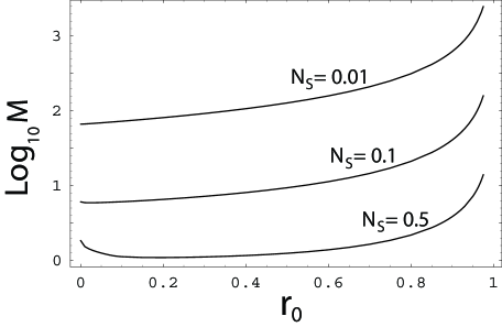
Figure 2: Number of signals $M$ (logarithmic scale) versus pit-reflectivity $r_{0}$. The curves refer to $N_{S}=0.01$, $0.1$ and $0.5$ photons. For each value of the energy $N_{S}$, we plot the critical number $M^{(N_{S})}(r_{0})$ as function of $r_{0}$. All the curves have an asymptote at $r_{0}=1$. For $N_{S}\gtrsim 2.5$ photons (curves not shown), we have another asymptote at $r_{0}=0$.

It is remarkable that, for low-energy signals ($N_{S}=0.01\div 1$ photons), the critical number $M^{(N_{S})}(r_{0})$ is finite for every $r_{0}\in[0,1)$. This means that, for ideal memories and low-energy signals, there always exists a finite number of signals $M^{(N_{S})}$ above which the quantum readout of the memory is more efficient than its classical readout. In other words, there is an EPR transmitter with $M>M^{(N_{S})}$ able to beat any classical transmitter with the same number of signals $M$. In the considered low-energy regime, $M^{(N_{S})}(r_{0})$ is relatively small for almost all the values of $r_{0}$, except for $r_{0}\rightarrow 1$ where $M^{(N_{S})}(r_{0})\rightarrow\infty$. In fact, for $r_{0}\simeq 1$, we derive $M^{(N_{S})}(r_{0})\simeq[4N_{S}(2N_{S}+1)(1-r_{0})]^{-1}$, which diverges at $r_{0}=1$. Such a divergence is expected, since we must have $P_{err}^{quant}=P_{err}^{class}=1/2$ for $r_{0}=r_{1}$ (see Appendix 0.A for details). Apart from the divergence at $r_{0}=1$, in all the other points $r_{0}\in[0,1)$, the critical number $M^{(N_{S})}(r_{0})$ decreases for increasing energy $N_{S}$ (see Fig. 2). In particular, for $N_{S}=1$ photon, we have $M^{(N_{S})}(r_{0})\simeq 1$ for most of the reflectivities $r_{0}$. In other words, for energies around one photon, a single TMSV state is sufficient to provide a positive gain for most of the ideal memories. However, the decreasing trend of $M^{(N_{S})}(r_{0})$ does not continue for higher energies ($N_{S}\geq 1$). In fact, just after $N_{S}=1$, $M^{(N_{S})}(r_{0})$ starts to increase around $r_{0}=0$. In particular, for $N_{S}\geq 1$, we can derive $M^{(N_{S})}(0)\simeq(\ln 2)[2\ln(1+N_{S})-N_{S}]^{-1}$, which is increasing in $N_{S}$, and becomes infinite at $N_{S}\simeq 2.5$. As a consequence, for $N_{S}\gtrsim 2.5$ photons, we have a second asymptote appearing at $r_{0}=0$ (see Appendix 0.B for details). This means that the use of high-energy signals ($N_{S}\gtrsim 2.5$) does not assure positive gains for memories with extremal reflectivities $r_{0}=0$ and $r_{1}=1$.

4 Conclusion

In conclusion, we have considered the basic model of digital memory studied in Ref. [57], which is composed of beam splitter mirrors with different reflectivities. Adopting this model, we have compared an EPR transmitter with classical sources for fixed signal profiles, finding positive information gains for memories with high land-reflectivities ($r_{1}\gtrsim 0.8$). Analytical results can be derived in the limit of ideal land-reflectivity ($r_{1}=1$) which defines the regime of ideal memories. In this case, by fixing the mean number of photons per signal mode (local energy constraint), we have computed the critical number of signals after which an EPR transmitter gives positive information gains. For low-energy signals ($0.01\div 1$ photons) this critical number is finite and relatively small for every ideal memory. In particular, an EPR transmitter with one TMSV state can be sufficient to achieve positive information gains for almost all the ideal memories. Finally, our results corroborate the outcomes of Ref. [57] providing an alternative study which considers a local energy constraint instead of a global one. As discussed in Ref. [57], potential applications are in the technology of optical digital memories and involve increasing their data-transfer rates and storage capacities.

Appendix 0.A General asymptote at $r_{0}=1$

According to Fig. 2, the critical number $M^{(N_{S})}(r_{0})$ diverges for $r_{0}\rightarrow 1$. Let us analyze the behavior of $G$ around the singular point $r_{0}=1$, by setting $r_{0}=1-\varepsilon$ and expanding $G$ for $\varepsilon\rightarrow 0^{+}$. It is easy to check that, for every $N_{B}$, we have $G>0$ if and only if $M>[4N_{S}(2N_{S}+1)\varepsilon]^{-1}$. In particular, in the absence of thermal noise ($N_{B}=0$), we have

$$G=\frac{MN_{S}(4MN_{S}-1)\varepsilon^{2}}{8\ln 2}+O(\varepsilon^{3})~{},$$ (4)

which is positive if and only if $M>(4N_{S})^{-1}$.

Proof.  Note that $G>0$ if and only if $\Delta:=\mathcal{Q}(M,N_{S})-\mathcal{C}(M,N_{S})<0$. Let us expand $\Delta=\Delta(M,N_{S},N_{B},1-\varepsilon)$ at the first order in $\varepsilon$. For a given $N_{B}>0$, we have $\Delta=\frac{1}{2}\left[\left(MN_{B}\varepsilon\right)^{1/2}-M(N_{B}+N_{S}+2N_{B}N_{S})\varepsilon\right]+O(\varepsilon^{3/2})$, which is negative if and only if

$$M>\frac{N_{B}}{(N_{B}+N_{S}+2N_{B}N_{S})^{2}\varepsilon}:=\kappa(N_{B})~{}.$$

Notice that $\kappa(N_{B})$ is maximum for $N_{B}^{\ast}=N_{S}(1+2N_{S})^{-1}$. Then, for every $N_{B}>0$, we have $\Delta<0$ if and only if

$$M>\kappa(N_{B}^{\ast})=\frac{1}{4N_{S}(2N_{S}+1)\varepsilon}~{}.$$ (5)

Now, let us consider the particular case of $N_{B}=0$. In this case, we have the first-order expansion $\Delta=\left(MN_{S}\right)^{1/2}[1-2\left(MN_{S}\right)^{1/2}]\varepsilon/4+O(\varepsilon^{2})$, or equivalently the second-order expansion of $G$ given in Eq. (4). It is clear that $\Delta<0$, i.e., $G>0$, when $M>1/4N_{S}$. However, this condition is less restrictive than the one in Eq. (5) which, therefore, can be extended to every $N_{B}\geq 0$. $\blacksquare$

Appendix 0.B High-energy asymptote at $r_{0}=0$

Let us analyze the behavior of $M^{(N_{S})}(r_{0})$ for $N_{S}\geq 1$ and $r_{0}=0$. One can check that, for $N_{S}\geq 1$, the greatest value of $M^{(N_{S})}(0)$ occurs when $N_{B}=0$. In this case, i.e., for $r_{0}=N_{B}=0$ and $r_{1}=1$, we have $\mathcal{Q}(M,N_{S})=[\left(1+N_{S}\right)^{-2M}]/2$, and

$$\mathcal{C}(M,N_{S})=\frac{1-\sqrt{1-e^{-MN_{S}}}}{2}\overset{M\gg 1}{\longrightarrow}\frac{e^{-MN_{S}}}{4}:=\mathcal{C}^{\infty}.$$

Let us consider the critical value $M^{(N_{S})}(0)$ of $M$ such that $G(M,N_{S})=0$, which is equivalent to $\mathcal{Q}=\mathcal{C}$. We also consider the value $\tilde{M}$ such that $\mathcal{Q}=\mathcal{C}^{\infty}$. Since $\mathcal{C}^{\infty}\leq\mathcal{C}$, we have that $M^{(N_{S})}(0)\geq\tilde{M}$. Actually, we find that $M^{(N_{S})}(0)\simeq\tilde{M}$ with very good approximation when $N_{S}\geq 1$ (see Fig. 3). Then, for every $N_{S}\geq 1$, we can set $M^{(N_{S})}(0)\simeq(\ln 2)\left[2\ln(1+N_{S})-N_{S}\right]^{-1}$. The latter quantity becomes infinite for $2\ln(1+N_{S})=N_{S}$, i.e., for $N_{S}\gtrsim 2.51$ photons.

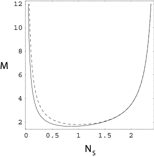
Figure 3: Minimum number of signals $M$ versus energy $N_{S}$. The solid curve represents $M^{(N_{S})}(0)$ while the dashed curve represents $\tilde{M}$. Note that the minimum number of signals is actually given by $\left\lceil M\right\rceil$ where $\left\lceil\cdots\right\rceil$ is the ceiling function.

References

- [1] M. A. Nielsen and I. L. Chuang, Quantum Computation and Quantum Information (Cambridge University Press, Cambridge, 2000).
- [2] C. Weedbrook, S. Pirandola, R. Garcia-Patron, N. J. Cerf, T. C. Ralph, J. H. Shapiro, and S. Lloyd, Gaussian Quantum Information, preprint arXiv:1110.3234
- [3] S. L. Braunstein and A. K. Pati, Quantum Information Theory with Continuous Variables, (Kluwer Academic, Dordrecht, 2003).
- [4] S. L. Braunstein and P. van Loock, Rev. Mod. Phys. 77, 513 (2005).
- [5] A. Ferraro, S. Olivares, and M. Paris, Gaussian states in quantum information, ISBN 88-7088-483-X (Biliopolis, Napoli, 2005).
- [6] J. Eisert, and M.B. Plenio, Int. J. Quant. Inf. 1, 479 (2003).
- [7] A. Furusawa et al., Science 282, 706 (1998).
- [8] S. L. Braunstein, and H. J. Kimble, Phys. Rev. Lett. 80, 869 (1998).
- [9] T. C. Ralph, Optics Letters 24, 348 (1999).
- [10] S. Pirandola, S. Mancini, D. Vitali, and P. Tombesi, Phys. Rev. A 68, 062317 (2003).
- [11] S. D. Bartlett and W. J. Munro, Phys. Rev. Lett. 90, 117901 (2003).
- [12] J. Sherson, H. Krauter, R. K. Olsson, B. Julsgaard, K. Hammerer, I. Cirac, and E. S. Polzik, Nature 443, 557 (2009).
- [13] P. van Loock, and S. L. Braunstein, Phys. Rev. Lett. 84, 3482 (2000).
- [14] S. Pirandola and S. Mancini, Laser Physics 16, 1418 (2006).
- [15] S. Pirandola, S. Mancini, D. Vitali, and P. Tombesi, J. Mod. Opt. 51, 901 (2004).
- [16] S. Pirandola, Int. J. Quant. Inf. 3, 239 (2005).
- [17] S. Pirandola, S. Mancini, and D. Vitali, Phys. Rev. A 71, 042326 (2005).
- [18] P. van Loock and S. L. Braunstein, Phys. Rev. A 61, 010302(R) (1999).
- [19] N. Takei, H. Yonezawa, T. Aoki, and A. Furusawa, Phys. Rev. Lett. 94, 220502 (2005).
- [20] S. Pirandola, D. Vitali, P. Tombesi, and S. Lloyd, Phys. Rev. Lett. 97, 150403 (2006).
- [21] N. J. Cerf, M. Levy, and G. van Assche, Phys. Rev. A 63, 052311 (2001).
- [22] F. Grosshans, and P. Grangier, Phys. Rev. Lett. 88, 057902 (2002).
- [23] C. Weedbrook, A. M. Lance, W. P. Bowen, T. Symul, T. C. Ralph, and P. K. Lam, Phys. Rev. Lett. 93, 170504 (2004).
- [24] C. Weedbrook, C., A. M. Lance, W. P. Bowen, T. Symul, T. C. Ralph, and P. K. Lam, Phys. Rev. A 73, 022316 (2006).
- [25] C. Weedbrook, S. Pirandola, S. Lloyd, T. C. Ralph, Phys. Rev. Lett. 105, 110501 (2010)
- [26] S. Pirandola, S. Mancini, S. Lloyd, and S. L. Braunstein, Nature Physics 4, 726 (2008).
- [27] S. Pirandola, S. Mancini, S. Lloyd, and S. L. Braunstein, Proc. SPIE 7092, 709215 (2008).
- [28] S. Lloyd and S. L. Braunstein, Phys. Rev. Lett. 82, 1784 (1999).
- [29] D. Gottesman, A. Kitaev, and J. Preskill, Phys. Rev. A 64, 012310 (2001).
- [30] B. C. Travaglione and G. J. Milburn, Phys. Rev. A 66, 052322 (2002).
- [31] S. Pirandola, S. Mancini, D. Vitali, and P. Tombesi, Europhys. Lett. 68, 323 (2004).
- [32] S. Glancy and E. Knill, Phys. Rev. A 73, 012325 (2006).
- [33] S. Pirandola, S. Mancini, D. Vitali, and P. Tombesi, J. Phys. B: At. Mol. Opt. Phys. 39, 997 (2006).
- [34] S. Pirandola, S. Mancini, D. Vitali, and P. Tombesi, Eur. Phys. J. D 37, 283-290 (2006).
- [35] R. Raussendorf, and H. J. Briegel, Phys. Rev. Lett. 86, 5188 (2001).
- [36] N. C. Menicucci, P. van Loock, M. Gu, C. Weedbrook, T. C. Ralph, and M. A. Nielsen, Phys. Rev. Lett. 97, 110501 (2006)
- [37] J. Zhang and S. L. Braunstein, Phys. Rev. A 73, 032318 (2006).
- [38] S. T. Flammia, N. C. Menicucci, and O. Pfister, J. Phys. B 42, 114009 (2009).
- [39] A. S. Holevo, Prob. of Inf. Transm. 43, 1 (2007).
- [40] S. Pirandola, S. L. Braunstein, and S. Lloyd, Phys. Rev. Lett. 101, 200504 (2008).
- [41] S. Pirandola, S. L. Braunstein, S. Lloyd, Lecture Notes in Computer Science 5906, 47-55 (2009).
- [42] I. Devetak, IEEE Trans. Inf. Theory 51, 44 (2005).
- [43] I. Devetak and A. Winter, Phys. Rev. Lett. 93, 080501 (2004).
- [44] I. Devetak and A. Winter, Proc. R. Soc. Lond. A 461, 207 (2005).
- [45] S. Pirandola, R. Garcıa-Patron, S. L. Braunstein, and S. Lloyd, Phys. Rev. Lett. 102, 050503 (2009).
- [46] R. García-Patrón, S. Pirandola, S. Lloyd, J. H. Shapiro, Phys. Rev. Lett. 102, 210501 (2009).
- [47] S. Pirandola, S. L. Braunstein, S. Mancini, and S. Lloyd, Europhys. Lett. 84, 20013 (2008).
- [48] S. Pirandola, S. L. Braunstein, S. Lloyd, and S. Mancini, IEEE J. of Selected Topics in Quant. El. 15, 1570-1580 (2009).
- [49] A. Einstein, B. Podolsky, and N. Rosen, Phys. Rev. 47, 777 (1935).
- [50] For two bosonic modes, and , with quadratures , , and , one can define the two operators (relative position) and (total momentum). Then, the system has EPR correlations (in these operators) if , where is the variance, and is the standard quantum limit ( in this paper.) A bosonic system with EPR correlations is entangled, but the contrary is not necessarily true. In today’s quantum optics labs, the EPR correlations represent the standard type of continuous variable entanglement. These correlations are usually generated via spontaneous parametric down conversion.
- [51] S.-H. Tan, B. I. Erkmen, V. Giovannetti, S. Guha, S. Lloyd, L. Maccone, S. Pirandola, and J. H. Shapiro, Phys. Rev. Lett. 101, 253601 (2008).
- [52] S. Lloyd, Science 321, 1463 (2008).
- [53] J. H. Shapiro and Seth Lloyd, New J. Phys. 11, 063045 (2009).
- [54] S. Guha and B. Erkmen, Phys. Rev. A 80, 052310 (2009).
- [55] A. R. Usha Devi and A. K. Rajagopal, Phys. Rev. A 79, 062320 (2009).
- [56] H. P. Yuen, and R. Nair, Phys. Rev. A 80, 023816 (2009).
- [57] S. Pirandola, Phys. Rev. Lett. 106, 090504 (2011).
- [58] E. C. G. Sudarshan, Phys. Rev. Lett. 10, 277 (1963).
- [59] R. J. Glauber, Phys. Rev. 131, 2766 (1963).
- [60] C. W. Helstrom, Quantum detection and estimation theory (Academic Press, New York, 1976).
- [61] C. A. Fuchs and J. V. de Graaf, IEEE Trans. Inf. Theory 45, 1216 (1999).
- [62] C. Fuchs, PhD thesis (Univ. of New Mexico, Albuquerque, 1995).
- [63] K. M. R. Audenaert et al., Phys. Rev. Lett. 98, 160501 (2007).
- [64] J. Calsamiglia et al., Phys. Rev. A 77, 032311 (2008).
- [65] M. Nussbaum and A. Szkoła, Annals of Statistics 37, 1040-1057 (2009).
- [66] K. M. R. Audenaert, M. Nussbaum, A. Szkoła, and F. Verstraete, Comm. Math. Phys. 279, 251–283 (2008).
- [67] S. Pirandola and S. Lloyd, Phys. Rev. A 78, 012331 (2008).
- [68] S. Pirandola, A. Serafini, and S. Lloyd, Phys. Rev. A 79, 052327 (2009).
- [69] To be precise, the critical number is a solution of the equation . From this real value we derive the minimum number of signals (which is an integer) by taking its ceiling function .