Coupled DEM-LBM method for the free-surface simulation of heterogeneous suspensions

Abstract

The complexity of the interactions between the constituent granular and liquid phases of a suspension requires an adequate treatment of the constituents themselves. A promising way for numerical simulations of such systems is given by hybrid computational frameworks. This is naturally done, when the Lagrangian description of particle dynamics of the granular phase finds a correspondence in the fluid description. In this work we employ extensions of the Lattice-Boltzmann Method for non-Newtonian rheology, free surfaces, and moving boundaries. The models allows for a full coupling of the phases, but in a simplified way. An experimental validation is given by an example of gravity driven flow of a particle suspension.

1 Introduction

Free-surface flows of heterogeneous suspensions are abundant in nature and technical applications. In principle they are multiphase materials composed of a mixture of a liquid and of solid grains of various size. A multitude of interaction mechanisms between these two phases renders the problem of their description rather difficult. For example very small grains are bounded to the liquid by electrostatic forces, while bigger ones interact mainly by viscous forces coussot1997mudflow . Additionally, inter-grain interactions give rise to the typical complex behavior of granular matter. Often grains have a broad size distribution spanning over several orders of magnitude. Two well known examples are mixtures of mud with sand and rocks as well as suspensions of Portland cement, sand, and larger aggregates, also known as fresh concrete. While the latter is used for construction purposes Ferraris2001 , the former gives rise to devastating debris flows Iverson1997 .

The simulation of such materials is based either on continuum Nott2006 ; Savage1989 or on particle methods Campbell1995 , depending on whether the investigated effects arise from the physics of the fluid or the granular phase. Continuum models are appropriate when the rheological behavior of the material can be captured by rheometry techniques and phenomenological constitutive laws. However, many physical phenomena are eluded by this approach such as size and phase segregation. Examples can be found in concrete casting, where improper mixing or vibration leads to inhomogeneities in the physical properties of the hardened concrete. In debris flows, size segregation leads to locally changing flow properties. A flow front rich of large grains with high destructive power is commonly observed, followed by a fluid in a more homogeneous tail. Describing this situation by continuum methods is quite difficult or even physically inappropriate Iverson . With particle methods, such as the Discrete Element Method (DEM), these phenomena can be naturally captured, which makes them an ideal tool for the study of the complex behavior of granular materials.

A complete simulation tool requires a combination of both continuum and particle description, which poses serious challenges from a computational point of view. If granular and fluid phases are fully coupled, grains represent an irregular and discontinuous boundary for the fluid domain. The relative motion of the phases complicates the picture further, because it requires the management of continuously evolving interfaces. For these reasons, traditional CFD solvers such as the standard Finite Element or Finite Volume methods, have enormous difficulties to tackle the issue. An attractive alternative is given by the Lattice-Boltzmann Method (LBM) He1997 ; Succi2001 , because of its extreme flexibility in the treatment of elaborate boundary conditions, its ease of implementation in parallel computing and its superior scaling when compared to traditional solvers. For these reasons, much effort has been payed to develop of a framework for particle-fluid systems combining the advantages of LBM and DEM. The early works in this field are due to Ladd Ladd1994 ; Ladd1994a ; Ladd2001 , who first coupled LBM and boundaries with imposed velocity. The basic model was enhanced by the use of the Immersed Boundary Method Feng2004 ; Owen2011 ; Leonardi2012a ; Leonardi2012 , by the inclusion of turbulence modeling Feng2007 and extended further to the simulation of non-Newtonian rheology models Ginzburg2001 ; Vikhansky2008 ; Leonardi2011 and for free-surface flows Korner2005 ; Svec2012 . Drawbacks of an approach based on the LBM are its limitation to low-Mach and relatively low-Reynolds flows, and the necessity to rely on a regular grid, since irregular grids are known to produce a complicated formalism and sometimes to lower the accuracy Ubertini2005 .

The paper is organized as follows: First a classification of particle suspensions by scales and types of physical interactions is given, before we explain how the dynamics of the different phases is addressed. In Sec. 3 we summarize the DEM approach for the granular phase, followed by a section with a comprehensive description of the LBM solver for the fluid phase. Sec. 5 explains necessary extensions to the LBM for the simulation of suspensions like fluid-particle interaction, non-Newtonian rheology or the representation of free surfaces. The experimental validation of the described model completes the manuscript in Sec. 6, followed by a brief summary.

2 Dynamics of Suspensions

The contribution of grains to the mechanics of the mixture can be of different nature depending, among other factors, on the grain size distribution. For a phenomenological classification, we use the term small scale when electrostatic forces are dominant, medium scale when viscous forces prevail, and large scale when inter-particle collisional forces dominate coussot1997mudflow . Note that the length-scales defined by grain size are by no means absolute, but depend on other parameters such as the concentration of particles, the viscosity of the liquid, and the state of the system, since the same material can exhibit different behaviors when sheared at different rates.

Small scale grain dynamics is governed mainly by interactions of electrostatic nature, e.g. Van der Waals forces. This finer part of the grains, together with water, forms a colloidal dispersion. A complete description of this kind of material can be found elsewhere russel1992colloidal . For practical purposes, the mechanics of colloidal dispersions is reproduced by continuum methods. A non-Newtonian model, however, is generally required, since colloidal dispersions can exhibit both shear-thinning behavior and plastic properties. In this work we choose to employ the Bingham plastic, a fluid model with a yield stress, well-known for its wide applicability Roussel2007 ; Whitehouse2000 . It is described as

$$\left\{\begin{array}[]{l l}\dot{\gamma}=0&\quad\textrm{if fluid does not yield}\ (\sigma<\sigma_{y}),\\ \sigma=\sigma_{y}+\mu_{pl}\dot{\gamma}&\quad\textrm{if fluid flows}\ (\sigma>\sigma_{y}),\\ \end{array}\right.\$$ (1)

where $\dot{\gamma}$ is the magnitude of the shear rate tensor, and $\mu_{pl}$, $\sigma_{y}$ denote plastic viscosity and yield stress. In analogy to Newtonian fluids, an apparent viscosity (from now on, simply called viscosity) can be locally defined as the ratio of shear rate and shear stress

$$\mu_{app}=\sigma/\dot{\gamma}=\mu_{pl}+\frac{\sigma_{y}}{\dot{\gamma}}.$$ (2)

As the shear rate $\dot{\gamma}$ approaches zero, the viscosity becomes infinite, giving a simple but efficient way to model plastic behavior.

Medium scale grains are sufficiently big to elude the effects of microscopic electrostatic forces and therefore need a different numerical treatment. For them the hydrodynamic effects due to the viscous nature of the fluid become dominant. In analogy to the smaller scale, grains can be homogenized in the fluid. Obtaining an appropriate rheological behavior of the final mixture is however more difficult. When experimental data is not available, the value of the viscosity can be approximated by constitutive relations. A review of these models can be found in Ref. Stickel2005 .

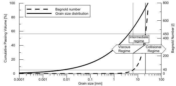
Figure 1: A typical grain size distribution and its effect on the dynamics of the mixture. Big grains fall in the collisional regime, small ones in the viscous regime. A transition zone exhibits hybrid characteristics. The Bagnold number is calculated with $\mu_{f}=1.0\ \textrm{Pa}\ \textrm{s}$, $\rho=1000\ \textrm{kg}/\textrm{m}^{3}$, $\lambda=1$, $\dot{\gamma}=100\ \textrm{s}^{-1}$

Large scale grain dynamics is dominated by collisions. When collisional effects are not damped by viscosity, grains give rise to collective phenomena, such as segregation, force percolation or shock waves Herrmann1998 . Bagnold defined a dimensionless number as the ratio of grain collisional and viscous stresses Bagnold1954 . It reads

$$\mathrm{Ba}=\frac{\rho_{s}d_{s}^{2}\lambda_{s}^{1/2}\dot{\gamma}}{\mu_{f}},$$ (3)

where $\mu_{f}$ is the dynamic viscosity of the liquid, $\dot{\gamma}$ the magnitude of the shear rate, $\rho_{s}$ and $d_{s}$ denote density and characteristic diameter of the grains, and $\lambda_{s}$ their linear concentration (function of the solid fraction $C_{s}$ as $\lambda_{s}=1/[(C_{s,max}/C_{s})^{1/3}-1]$ with $C_{s,max}$ the maximum solid fraction). As illustrated in Fig. 1, the Bagnold number is used to distinguish two different regimes, where different rheological laws are observed Geographie : Mixtures with $Ba<40$ are dominated by viscosity and therefore the shear stress grows proportionally to the shear rate. Mixtures with $Ba\geq 450$ are dominated by collisional effects and grains cannot be homogenized into a continuum description without a loss in the descriptive capabilities of the method. An intermediate range exists, where both effects are not negligible Hunt2002 .

The proposed model follows this classification to efficiently simulate and investigate suspensions. Small and medium scale grains are homogenized for a fluid formulation with a continuum Bingham model. Large scale grains are represented by a discrete description. The advantage of this method is that only a small portion grains is explicitly represented. This fraction is representative both in terms of mass and influence on the rheology of system.

3 Dynamics of the granular phase with the DEM

The granular phase is represented by the DEM, a well-established method for granular systems Bicanic2007a . Every grain $p$ is characterized as a Lagrangian element, with translation $\mathbf{x}_{p}$ and rotation $\mathbf{\phi}_{p}$ as degrees of freedoms. It is subjected to multiple interactions that lead to a resultant force $\mathbf{F}_{p}$ and moment $\mathbf{M}_{p}$. These interactions can either be due to collisions, hydrodynamics or volumetric forces and are functions of position, orientation and velocity of the particles: $\mathbf{F}_{p}=\mathbf{F}_{p}\left(\mathbf{x}_{p},\dot{\mathbf{x}}_{p},\mathbf{\phi}_{p},\dot{\mathbf{\phi}}_{p}\right)$, $\mathbf{M}_{p}=\mathbf{M}_{p}\left(\mathbf{x}_{p},\dot{\mathbf{x}}_{p},\mathbf{\phi}_{p},\dot{\mathbf{\phi}}_{p}\right)$.

In the simplest case, DEM particles have spherical shape allowing for fast contact detection and calculation of the overlap $\xi_{p,q}$ between particles $p$ and $q$ namely

$$\xi_{p,q}=||\mathbf{d}_{p,q}||-R_{p}-R_{q}.$$ (4)

Here $\mathbf{d}_{p,q}$ denotes the distance between the center of the spheres with radii $R_{p}$, $R_{q}$. Unfortunately, for most practical applications spheres can only be used as a first approximation of the real particle shape. Note that spheres exhibit artificial mixing and rolling behavior, which is absent in natural system that are not composed of spheres. To overcome these effects we use composite elements, created by aggregating a set of spherical particles. While preserving the simplicity of the contact calculation, composite elements allow for a more realistic representation of granular effects, in particular in the limit of dense concentrations.

Particle-particle interactions are written as the outcome of collisional events between particles. Although particles are geometrically described as rigid spheres, the overlap $\xi_{p,q}$ between particles $p$ and $q$ is used to calculate collisional forces and to represent the elastic deformation. We use the law for elastic spheres,

$$\mathbf{F}^{n}_{p,q}=\frac{2}{3}\frac{Y\sqrt{R_{eff}}}{\left(1-\nu^{2}\right)}\left(\xi_{p,q}^{3/2}+A\sqrt{\xi_{p,q}}\frac{d\xi_{p,q}}{dt}\right)\mathbf{n}_{p,q},$$ (5)

where $Y$ and $\nu$ are the Young modulus and the Poisson’s ratio of the material, $A$ is a damping constant Brilliantov1996 , $R_{eff}$ the effective radius defined as $R_{eff}=R_{p}R_{q}/(R_{p}+R_{q})$ and $\mathbf{n}_{p,q}$ the normal vector of the contact surface. The tangential contact force is considered to be proportional to the component of the relative velocity of the two spheres laying on the contact surface $\mathbf{u}^{t}_{rel}$ as

$$\mathbf{F}^{t}_{p,q}=-\textrm{sign}\left(\mathbf{u}^{t}_{rel}\right)\cdot\textrm{min}\left(\eta||\mathbf{u}^{t}_{rel}||,\mu_{d}||\mathbf{F}^{n}_{p,q}||\right)\mathbf{t}_{p,q},$$ (6)

with the tangential shear viscosity coefficient $\eta$ and the dynamic friction coefficient $\mu_{d}$, thus including Coulomb friction. The tangential unit vector $\mathbf{t}_{p,q}$ is obtained normalizing the tangential relative velocity. Wall contacts are calculated in a similar fashion.

The time evolution of the system is solved by integrating Newton’s second law,

$$m_{p}\ddot{\mathbf{x}}_{p}=\mathbf{F}_{p}, \mathbf{J}_{p}\ddot{\mathbf{\phi}}_{p}=\mathbf{M}_{p}-\dot{\mathbf{\phi}}_{p}\times\left(\mathbf{J}_{p}\dot{\mathbf{\phi}}_{p}\right).$$ (7)

While the translational motion is naturally solved in system coordinates, the rotational motion requires additional considerations. We use quaternion algebra rather that Euler angles to represent the orientation of the elements, and calculate and invert rotation matrices without singularities Carmona2008 . Newton’s equations in the body-fixed reference frame produce $6\times N$ scalar equation, where $N$ is the number of elements. The Gear predictor-corrector differential scheme is used to integrate them Gear1971 . During the predictor step, tentative values for particle position, orientation and their derivatives are computed, using a Taylor expansion of the previous time step values. The predicted values are then used to check for contacts, compute collisional forces and solve Newton’s equations of motion. For the corrector step, the difference between the predicted values for acceleration and their counterpart resulting from Newton’s equation is computed. This difference is used to calculate the new corrected values for position, orientation and their derivatives.

The DEM time step should be small enough to resolve the particle contacts. If $t_{c}$ is the collision time, then ${\Delta t}^{\textrm{DEM}}\ll t_{c}$, usually ${\Delta t}^{\textrm{DEM}}<0.1t_{c}$. The collision time can be estimated for a Hertzian contact as

$$t_{c}=2.5\left(\frac{m_{eff}^{2}}{k^{2}||\mathbf{u}^{n}_{rel}||}\right)^{\frac{1}{5}}\textrm{, with} k=\frac{8}{15}\frac{Y}{1-\nu^{2}}\sqrt{R_{eff}},$$ (8)

where $m_{eff}=m_{p}m_{q}/\left(m_{p}+m_{q}\right)$ is the effective mass and $\mathbf{u}^{n}_{rel}$ denotes the normal relative velocity at the contact point at the beginning of the collision.

4 Fluid dynamics with the LBM

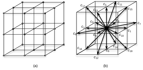
Figure 2: a) The regular space discretization of the lattice. b) The 19 discrete velocities allowed in the D3Q19 lattice configuration

The DEM described in the previous section is coupled with the LBM for solving the fluid phase. LBM has been evolving very fast in the last two decades and is considered to be one of the most attractive alternatives to traditional CFD solvers, especially when problems feature complex boundary conditions. It originates from the Boltzmann kinetic theory for the evolution of molecular systems Benzia1992 ; Chen1998 . The fluid is described using a distribution function, $f(\mathbf{x},\mathbf{c},t)$, defined as the probability density of finding molecules with velocity $\mathbf{c}$ at a location $\mathbf{x}$ and at a given time $t$.

In the LBM, the velocity space is discretized by a finite number of velocity vectors, $\mathbf{c}_{i}$, such that $f_{i}(\mathbf{x},t)\equiv f(\mathbf{x},\mathbf{c}_{i},t)$. We choose to employ the D3Q19 lattice cell configuration ($3$ dimensions and $19$ velocities, see Fig. 2), which provides the required symmetries to correctly recover the incompressible Navier-Stokes equations. In this work, for simplicity, we use dimensionless lattice units ($\delta_{x,y,z}=1,\ \delta_{t}=1$).

The reconstruction of macroscopic physical variables such as density $\rho_{f}$ and velocity $\mathbf{u}_{f}$ can be done at every location $\mathbf{x}$ and time $t$ by computing the first two moments of the distribution function $f_{i}(\mathbf{x},t)$

$$\rho_{f}(\mathbf{x},t)=\sum\limits_{i}f_{i}(\mathbf{x},t), \mathbf{u}_{f}=\sum\limits_{i}f_{i}(\mathbf{x},t)\mathbf{c}_{i}/\rho_{f}(\mathbf{x},t).$$ (9)

The distribution function evolves according to the Lattice Boltzmann Equation (LBE), which is written

$$f_{i}(\mathbf{x}+\mathbf{c}_{i},t+1)=f_{i}(\mathbf{x},t)+\Omega_{i}(\mathbf{x},t).$$ (10)

$\Omega_{i}$ represents the collision operator, which in our case corresponds to the linear approximation given by Bhatnagar-Gross-Krook Bhatnagar1954 ,

$$\Omega_{i}(\mathbf{x},t)=\frac{f_{i}^{eq}(\mathbf{u}_{f},\rho_{f})-f_{i}(\mathbf{x},t)}{\tau(\mathbf{x},t)},$$ (11)

where $\tau$ is the relaxation time and $f_{i}^{eq}$ is the equilibrium distribution function. The relaxation time is directly related to the viscosity of the fluid

$$\mu_{f}(\mathbf{x},t)=\frac{\tau(\mathbf{x},t)-1/2}{3}.$$ (12)

For a Newtonian fluid, the relaxation time $\tau$ is a constant and global parameter. However, as stated in Sec. 2, in order to represent most suspensions, a non-Newtonian formulation should be employed. To do this, the relaxation time is treated as a local variable $\tau(\mathbf{x},t)$. The equilibrium distribution function $f_{i}^{eq}$ is an expansion in Hermite polynomials of the Maxwell-Boltzmann distribution in the limit of small velocities Shan1998 . Using the local macroscopic velocity $\mathbf{u}_{f}$ and density $\rho_{f}$, this yields

$$f_{i}^{eq}(\mathbf{u}_{f},\rho_{f})=\rho_{f}w_{i}\left(1+3\mathbf{c}_{i}\cdot\mathbf{u}_{f}+\frac{9}{2}\left(\mathbf{c}_{i}\cdot\mathbf{u}_{f}\right)^{2}-\frac{3}{2}\mathbf{u}_{f}\cdot\mathbf{u}_{f}\right),$$ (13)

where the weights $w_{i}$ are constants that ensure the recovering of the first and second moments of the distribution function (Eq. 9). For the D3Q19 lattice configuration they are

$$w_{i}=\left\{\begin{array}[]{l l}1/3&\quad\textrm{for}\ i=1\\ 1/18&\quad\textrm{for}\ i=2\textrm{...}7\\ 1/36&\quad\textrm{for}\ i=8\textrm{...}19.\\ \end{array}\right.\$$ (17)

To introduce an external force, we employ the scheme developed by Guo et al. Guo2002 , which consists in modifying Eq. 10 as

$$f_{i}(\mathbf{x}+\mathbf{c}_{i},t+1)=f_{i}(\mathbf{x},t)+\Omega_{i}(\mathbf{x},t)+F_{i}(\mathbf{x},t),$$ (18)

where $F_{i}(\mathbf{x},t)$ is an additional distribution function due to the force field $\mathbf{F}$, which can be calculated in a similar fashion as the equilibrium distribution,

$$F_{i}(\mathbf{x},t)=w_{i}\left(1-\frac{1}{2\tau}\right)\left[3\left(\mathbf{c}_{i}-\mathbf{u}_{f}\right)+9\mathbf{c}_{i}\left(\mathbf{c}_{i}\cdot\mathbf{u}_{f}\right)\right]\mathbf{F}.$$ (19)

With this technique, the computation of the macroscopic velocity field in Eq. 9 also needs to be modified,

$$\mathbf{u}_{f}=\left(\sum\limits_{i}f_{i}(\mathbf{x},t)\mathbf{c}_{i}+\mathbf{F}/2\right)/\rho_{f}(\mathbf{x},t).$$ (20)

The described approach reproduces the Navier-Stokes equations in the incompressible limit. The pressure is directly computable from the density as

$$P_{f}(\mathbf{x},t)=\rho_{f}(\mathbf{x},t)\cdot c_{s}^{2},$$ (21)

where $c_{s}$ is the speed of sound of the fluid, which corresponds to $c_{s}=1/\sqrt{3}$ (lattice units). The stability and accuracy of the LBM are guaranteed for small Mach numbers, $Ma\equiv||\mathbf{u}||/c_{s}\ll 1$.

For every time step one first calculates the macroscopic variables, using Eq. 9, and the corresponding equilibrium distribution, from Eq. 13. Then, one uses Eq. 10 to evolve the distribution function, which provides the new density and velocity of the fluid for the next time step. Being solved mostly at a local level, the scheme can be easily implemented in a parallel environment Monitzer2012 .

5 Extensions of the LBM for the simulation of suspensions

To widen the range of applicability of the model to heterogeneous suspensions, we need to incorporate a few more features. First, we introduce no-slip moving boundaries, necessary for the coupling with the DEM, and second, in Sec. 5.2, we extend the model to simulate free surfaces. Finally, Sec. 5.3 describes the method for non-Newtonian formulations.

5.1 Coupling with particles

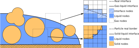
Figure 3: Sketch showing how particles or solid objects are discretized on the regular lattice. The free-surface is treated in a similar way, with a special type of nodes defining the interface

The coupling with the DEM and the treatment of no-slip boundary conditions are performed at a local level by modifying the LBE. Lattice nodes are divided into fluid and solid nodes, the latter ones representing particles and walls (see Fig. 3). Solid nodes are inactive, i.e. on them the LBE is not solved. No-slip is performed with the so-called bounce-back rule: every time a distribution function $f_{i}(\mathbf{x},t)$ is streaming in the direction $i$ towards a solid node, it gets reflected back in the opposite direction $i^{\prime}$. If the boundary is moving, the reflected distribution needs to be corrected as

$$f_{i^{\prime}}(\mathbf{x},t+1)=f_{i}(\mathbf{x},t)-6w_{i}\rho\mathbf{u}_{w}\cdot\mathbf{c}_{i},$$ (22)

where $\mathbf{u}_{w}$ is the local velocity of the wall at the bounce-back location. If the wall represents the surface of a particle, the local velocity can be obtained as

$$\mathbf{u}_{w}=\mathbf{u}_{p}+\mathbf{r}_{w}\times\mathbf{\omega}_{p},$$ (23)

where $\mathbf{u}_{p}$ and $\mathbf{\omega}_{p}$ are the linear and angular velocity of the particle, and $\mathbf{r}_{w}$ is the vector connecting its center of mass with the bounce-back location. The momentum exchange experienced by the reflected distribution can also be used to compute the force exerted on the wall when integrated over all bounce-back locations,

$$\mathbf{F}_{p}=\sum\left(2f_{i}(\mathbf{x},t)-6w_{i}\rho_{f}\mathbf{u}_{w}\cdot\mathbf{c}_{i}\right)\mathbf{c}_{i}.$$ (24)

Solid boundaries treated this way are located halfway between solid and active nodes. This technique was developed for moving boundaries by Ladd Ladd1994 and Aidun and Lu Aidun1995 .

Particles move over a fixed, regular grid. Of course the node classification into fluid and solid is not fixed but needs to be updated. Following the particle motion, fluid nodes are created (deleted) in the wake (front) of moving particles. The macroscopic density and the velocity of the newly created nodes are calculated as the average over the values in the neighborhood as initial values for the distribution function $f_{i}(\mathbf{x},t)$ through Eq. 13. Deleted fluid nodes are converted to solid ones and therefore made inactive. Both processes introduce small variations in the global mass and momentum. However, due to the fact that all our simulations are performed in the incompressible limit (variation of density are very small), and that fluid nodes close to a particle possess nearly the same velocity as the particle, we expect these variations to be negligible. Another problem is the representation of the particle boundaries on the regular lattice, which leads to a zig-zag approximation of the spherical shapes. An alternative way to overcome these problems is the use of the Immersed Boundary Method Feng2004 or of a fictitious domain Glowinski1999 ; Glowinski2001 . Both methods are more precise and smooth the ill effects of particles traveling though the lattice. At the same time, they require additional computations and are therefore avoided following the spirit of this paper.

When two particles approach each other, the distance between the surfaces can become smaller than the lattice node spacing, resulting in an imprecise resolution of the collision process. To overcame this problem, we use the lubrication theory of Nguyen and Ladd Nguyen2002 . In this theory, when two particle are moving with a relative velocity $\mathbf{u}_{rel}$, the correction force

$$\mathbf{F}^{lub}_{p,q}=-6\mu_{f}||\mathbf{u}^{n}_{rel}||R_{eff}^{2}\left(1/s_{p,q}-1/d_{lub}\right)\mathbf{n}_{p,q},$$ (25)

is added, where $s_{p,q}=-\xi_{p,q}$ is the distance between the particle surfaces and $d_{lub}$ denotes a cut-off distance above which no force is computed.

5.2 Free surface representation

We employ the mass tracking algorithm described in Refs. Chen1998 ; Mendoza2010 which, despite its simplicity, leads to a stable and accurate surface evolution. Fluid nodes are further divided into liquid, interface and gas nodes: Liquid and interface nodes are considered active, and the LBE is solved. The remaining nodes are the gas nodes and are inactive, with no evolution equation. Liquid and gas nodes are never directly connected, but through an interface node (see Fig. 3).

An additional macroscopic variable for the mass $m_{f}(\mathbf{x},t)$ stored in a node is required, defined as

$$\left\{\begin{array}[]{l l}m_{f}(\mathbf{x},t)=\rho_{f}(\mathbf{x},t)&\quad\textrm{if the node is liquid,}\\ 0<m_{f}(\mathbf{x},t)<\rho_{f}(\mathbf{x},t)&\quad\textrm{if the node is interface,}\\ m_{f}(\mathbf{x},t)=0&\quad\textrm{if the node is gas.}\\ \end{array}\right.\$$ (29)

The mass is updated using the equation

$$m_{f}(\mathbf{x},t+1)=m_{f}(\mathbf{x},t)+\sum_{i}\alpha_{i}\left[f_{i^{\prime}}(\mathbf{x}+\mathbf{c}_{i},t)-f_{i}(\mathbf{x},t)\right],$$ (30)

where $\alpha_{i}$ is a parameter determined by the nature of the neighbor node in the $i$ direction,

$$\alpha_{i}=\left\{\begin{array}[]{l l}\frac{1}{2}\left[m_{f}(\mathbf{x},t)+m_{f}(\mathbf{x}+\mathbf{c}_{i},t)\right]&\quad\textrm{if the neighbor node is interface,}\\ 1&\quad\textrm{if the neighbor node is liquid,}\\ 0&\quad\textrm{if the neighbor node is gas.}\\ \end{array}\right.\$$ (34)

When the mass becomes zero ($m_{f}(\mathbf{x},t)=0$), the interface node is transformed into gas, with all liquid nodes connected to it becoming interface. Analogously, an interface node whose mass reaches the density ($m_{f}(\mathbf{x},t)=\rho_{f}(\mathbf{x},t)$) is transformed into liquid, and all connected gas nodes become interface. However, due to the discrete integration, these equalities are not in general satisfied. The surplus of mass is equally distributed to the neighboring interface nodes, conserving the total mass of the system.

Because gas nodes are not active, there are no distribution functions streaming from gas nodes to interface nodes. These missing distribution functions are computed from the macroscopic variables at the interface, atmospheric density $\rho_{atm}$ and interface velocity $\mathbf{u}_{int}$, as

$$f_{i^{\prime}}(\mathbf{x}+\mathbf{c}_{i^{\prime}},t+1)=f^{eq}_{i}(\mathbf{u}_{int},\rho_{atm})+f^{eq}_{i^{\prime}}(\mathbf{u}_{int},\rho_{atm})-f_{i}(\mathbf{x},t).$$ (35)

Note that this implies that gas nodes have the same macroscopic velocity as the connected interface nodes.

5.3 Bingham plastic rheology model

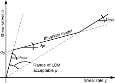
Figure 4: Representation of the rheology model employed for plastic fluids. The approximation of the Bingham model is limited by the maximum and minimum acceptable values for the relaxation time $\tau$ and therefore for the viscosity $\mu_{f}$

The presence of the small particle fraction in the fluid leads to non-Newtonian behavior, that needs to be considered. For the LBM this implies that the relaxation time $\tau$ is not a global parameter for the system, but rather $\tau=\tau(\mathbf{x},t)$. A non-linear dependency of viscosity, and thus of $\tau$, on the shear rate requires an explicit computation of the shear rate tensor. This can be done with ease in the LBM from the non-equilibrium part of the distribution functions,

$$\dot{\gamma}_{ab}(\mathbf{x},t)=\frac{3}{2\tau(\mathbf{x},t)}\sum_{i}\mathbf{c}_{i,a}\mathbf{c}_{i,b}\left(f_{i}(\mathbf{x},t)-f_{i}^{eq}(\mathbf{x},t)\right).$$ (36)

With the second invariant of the shear rate tensor

$$\Gamma_{\dot{\gamma}}(\mathbf{x},t)=\sum_{a}\sum_{b}\dot{\gamma}_{ab}\dot{\gamma}_{ab},$$ (37)

the magnitude of the shear rate is calculated as

$$\dot{\gamma}(\mathbf{x},t)=\sqrt{2\Gamma_{\dot{\gamma}}(\mathbf{x},t)}.$$ (38)

This can be included in any constitutive equation for purely viscous fluids. As outlined before (Sec. 2), we choose the Bingham constitutive model and get a new form of Eq. 12 for the explicit update of $\tau$,

$$\tau(\mathbf{x},t)=\frac{1}{2}+3\left(\mu_{pl}+\frac{\sigma_{y}}{\dot{\gamma}(\mathbf{x},t)}\right).$$ (39)

The accuracy and stability of LBM are guaranteed only over a certain range of values for $\tau$. This limits the applicability of Eq. 39, because $\tau$ diverges when $\dot{\gamma}\rightarrow 0$. Following Švec et al. Svec2012 , we use a simple solution to this problem, imposing that $\tau_{min}\leq\tau(\mathbf{x},t)\leq\tau_{max}$. Reasonable values for $\tau_{min}$ and $\tau_{max}$ are, respectively, $0.501$ and $3.5$. The constitutive equation arising from this approach is that of a tri-viscosity fluid (see Fig. 4). If $\mu_{f,min}<\mu_{pl}$ the model represents a bi-viscosity, and if $\mu_{f,max}\gg\mu_{pl}$, the approximation of the Bingham model is fair. With these extensions the model is complete and we can address examples.

6 Experimental validation by a gravity-driven flow

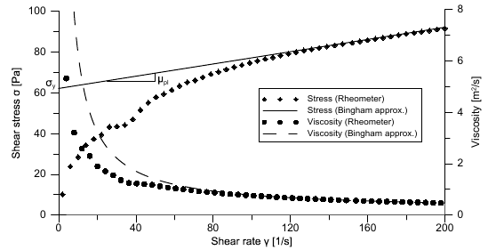
Figure 5: Rheology test on the fresh cement paste. A linear Bingham approximation is used to fit the data, obtaining $\mu_{pl}$ and $\sigma_{y}$

The capabilities of the model are shown by comparing with an experiment, featuring a free-surface flow of a suspension under the effect of gravity. We employ fresh concrete, since it poses all the challenges necessary to validate the method: a non-Newtonian rheology and an irregular granular phase. The cement paste is obtained with a commercial Portland cement of type CEM I $42.5\textrm{N}$. Water is added until a water/cement ratio of $0.4$ is reached. The rheology of the obtained paste is measured with a coaxial rotational viscometer Haake RV20. The measurement procedure consists in the uniform shearing of the paste at $200\ \textrm{s}^{-1}$ for $120\ \textrm{s}$, followed by a shear rate continuous ramp from $0$ up to $200\ \textrm{s}^{-1}$ occurring over $120\ \textrm{s}$ Geiker2002 . The obtained rheological curve is shown in Fig. 5.

The paste is mixed with $1000$ silica rounded pebbles with radius $R=4.0\div 8.0\ \textrm{mm}$. The total weight of the grains is $2.629\ \textrm{kg}$, and the density $\rho_{s}=2680\ \textrm{kg}/\textrm{m}^{3}$. The components are mixed in a bowl until homogenization and then vibrated for degassing. The final mixture is poured in a $150\times 150\ \textrm{mm}$ rectangular box, open on top and bottom and positioned over a wooden board inclined at $15^{\circ}$. The board surface is upholstered with sandpaper and wetted before the start of the test. The test is performed by steadily lifting the box, and letting the sample spread on the board under the sole effect of gravity. The flow falls in the intermediate regime (see Fig. 1). Collisional effects are therefore not dominant, but still important. The geometry of the test is illustrated in Fig. 6, and Fig. 7 (a) is a picture of the final deposition of the sample.

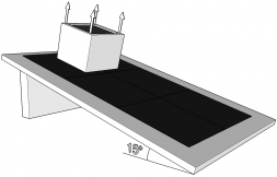
Figure 6: Experiment setup with an inclined plane of $933\times 700\textrm{mm}$. The internal size of the box is $150\times 150\ \textrm{mm}$. The dark gray area represents the surface covered by the sandpaper

The same environment is set up with a simulation on an LBM lattice of $350\times 250\times 80$ nodes, with the lattice spacing corresponding to $2.0\cdot 10^{-3}\textrm{m}$ in physical units. The initial configuration of the fluid is a cube with edge length of $0.15\textrm{m}$, corresponding to $75\times 75\times 75$ liquid nodes. The pebbles are represented with $1000$ discrete elements, each composed of 4 spheres with tetrahedral structure. The total number of spheres is $4000$. The box is represented by a set of moving walls and is set as solid boundary both for fluid and granular solvers. The lifting speed of the box is $0.15\textrm{m}/\textrm{s}$. The properties of the fluid are obtained from the viscometer data, as represented in Fig. 5. A good fit is obtained with a Bingham model with plastic viscosity $\mu_{pl}=0.15\ \textrm{Pa}\cdot\textrm{s}$ and yield stress $\sigma_{y}=62\ \textrm{Pa}$. The model is imprecise for lower shear rates, which is one of the limitations of the chosen linear approach. Fig. 8 shows the results of the simulation on the longitudinal cross section of the sample. The evolution of the shear rate and the particle distribution can be tracked continuously. The final shapes of the experimental and numerical solution are compared in Fig. 7 (c), showing excellent agreement.

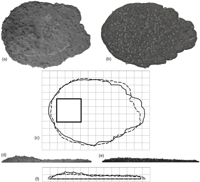
Figure 7: Final shape of the flowing mass. a,d) Numerical shape; b,e) Experimental shape. Fluid mass opacity in the numerical shape is lowered for a better visualization of particles; c,f) Comparison of numerical shape (solid line) and experimental shape (dashed line). The background grid has $5\textrm{cm}$ spacing

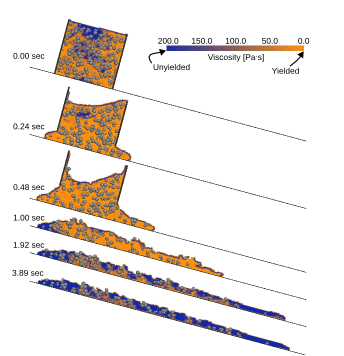
Figure 8: Dynamic viscosity contour on the longitudinal cross section of the simulation. Particles are represented in light gray and walls in dark gray. The yielded region of the fluid grows from a small portion close to the box walls to the whole sample during the first part of the simulation. When a new equilibrium is reached, the yielded region reduces and the flow is slowed

A good compromise between stability and speed is obtained with a time step of ${\Delta t}^{\textrm{LBM}}=3.0\cdot 10^{-5}\ \textrm{s}$. This sets the maximum allowable speed in the system as $0.667\ \textrm{m}/\textrm{s}$. The parameters in lattice units are then viscosity $\mu^{\textrm{LBM}}_{pl}=6.25\cdot 10^{-4}$, relaxation time $\tau^{\textrm{LBM}}_{y}=7.75\cdot 10^{-6}$, and gravity $||\mathbf{g}^{\textrm{LBM}}||=4.41\cdot 10^{-6}$. The simulation is stopped when $95\%$ of the fluid has reached the maximum viscosity. The total simulation time is 63 hours, with a parallel run on 4 cores with an Intel Xeon E5-1620 processor at 3.60 GHz..

7 Summary

In this paper a model for the simulation of the flow of suspensions was proposed. The multiscale nature of the model is justified by the different interaction mechanisms acting between the liquid and the granular phase. A practical mean of phenomenological classification of interactions is given by the Bagnold number: Small grains are considered to be governed by the viscous nature of the liquid and are modeled as part of the fluid phase itself with the use of a plastic non-Newtonian formulation. Grains with a sufficiently large size are dominated by collisional mechanisms. This is modeled with a two-way coupling between fluid and grains, along with the resolution of particle contacts.

The problem was solved with a hybrid of the Discrete Element Method for grains and the Lattice-Boltzmann Method for fluids. A combination of the most successful advances in these methods was employed. The mass-tracking algorithm allows an inexpensive way to simulate free surfaces, while the variable relaxation time formulation can reproduce non-Newtonian constitutive laws. The hydrodynamic interactions with the granular phase were fully solved with the bounce-back rule for coupling non-slip moving boundaries and fluid. The proposed model finds its best application in the simulation of real flows and in particular of heterogeneous suspensions with a granular phase that features a complete size distribution, due to its multiscale nature. The intrinsic advantages of the Lattice-Boltzmann solver, with its high- level performance and its relatively simple implementation make it a good choice for the fast development of such methods. Moreover, the core of the solver works at a local level, making the parallelization of the code easy and natural. Grain-grain interactions were solved with a Discrete Element Method. We assured that the scaling of the particle solver was not too far from the almost linear performances of the fluid solver. The Hertzian contact law was used, and a formulation for non-spherical particles was included. The capabilities of the approach were shown by comparing to an experimental free-surface flow of a fresh concrete sample. An excellent agreement between numerical and experimental data was found in the comparison of the final shape of the sample. The results of the simulation can provide insight into the mechanics of the flow. The spatial distribution of particles can be tracked, along with the variables of the flow: velocity, pressure, shear rate and viscosity.

Another challenging application of the model is the prediction of debris flows, which can hardly be assessed experimentally. Future works will focus on the rheology of debris materials and on the full simulation of events for deeper physical understanding, and on techniques for the design of effective protection measures.

- (1) Aidun, C.K., Lu, Y.: Lattice Boltzmann simulation of solid particles suspended in fluid. J. Stat. Phys. 81(1-2), 49–61 (1995). DOI 10.1007/BF02179967
- (2) Bagnold, R.A.: Experiments on a Gravity-Free Dispersion of Large Solid Spheres in a Newtonian Fluid under Shear. Proc. R. Soc. 225(1160), 49–63 (1954). DOI 10.1098/rspa.1954.0186
- (3) Benzi, R., Succi, S., Vergassola, M.: The lattice Boltzmann equation: theory and applications. Phys. Reports 222, 145–197 (1992). DOI 10.1016/0370-1573(92)90090-M
- (4) Bhatnagar, P.L., Gross, E.P., Krook, M.: A Model for Collision Processes in Gases. I. Small Amplitude Processes in Charged and Neutral One-Component Systems. Phys. Rev. 94(3), 511–525 (1954). DOI 10.1103/PhysRev.94.511
- (5) Bićanić, N.: Discrete Element Methods. In: E. Stein, R. de Borst, T.J.R. Hughes (eds.) Encycl. Comput. Mech., pp. 311–377. John Wiley & Sons, Ltd (2007). DOI 10.1002/0470091355.ecm006
- (6) Brilliantov, N., Spahn, F., Hertzsch, J., Pöschel, T.: Model for collisions in granular gases. Phys. Rev. E 53(5), 5382–5392 (1996). DOI 10.1103/PhysRevE.53.5382
- (7) Campbell, C.S., Cleary, P.W., Hopkins, M.: Large-scale landslide simulations: Global deformation, velocities and basal friction. J. Geophys. Res. 100(B5), 8267 (1995). DOI 10.1029/94JB00937
- (8) Carmona, H.A., Wittel, F.K., Kun, F., Herrmann, H.J.: Fragmentation processes in impact of spheres. Phys. Rev. E 77(5), 051,302 (2008). DOI 10.1103/PhysRevE.77.051302
- (9) Chen, S., Doolen, G.D.: Lattice Boltzmann Method for Fluid Flows. Annu. Rev. Fluid Mech. 30, 329–364 (1998). DOI 10.1146/annurev.fluid.30.1.329
- (10) Coussot, P.: Mudflow rheology and dynamics. A. A. Balkema, Rotterdam (1997)
- (11) Feng, Y.T., Han, K., Owen, D.R.J.: Coupled lattice Boltzmann method and discrete element modelling of particle transport in turbulent fluid flows: Computational issues. Int. J. Numer. Methods Eng. 72(1), 1111–1134 (2007). DOI 10.1002/nme.2114
- (12) Feng, Z.G., Michaelides, E.E.: The immersed boundary-lattice Boltzmann method for solving fluid-particles interaction problems. J. Comput. Phys. 195(2), 602–628 (2004). DOI 10.1016/j.jcp.2003.10.013
- (13) Ferraris, C.F., Obla, K.H., Hill, R.: The influence of mineral admixtures on the rheology of cement paste and concrete. Cem. Concr. Res. 31(2), 245–255 (2001). DOI 10.1016/S0008-8846(00)00454-3
- (14) Gear, C.W.: The automatic integration of ordinary differential equations. Commun. ACM 14(3), 176–179 (1971). DOI 10.1145/362566.362571
- (15) Geiker, M.R., Brandl, M., Thrane, L.N., Bager, D.H., Wallevik, O.: The effect of measuring procedure on the apparent rheological properties of self-compacting concrete. Cem. Concr. Res. 32(11), 1791–1795 (2002). DOI 10.1016/S0008-8846(02)00869-4
- (16) Ginzburg, I., Steiner, K.: Free surface Lattice-Boltzmann method to model the filling of expanding cavities by Bingham Fluids. Philos. Trans. R. Soc. 360(1792), 453–466 (2001). DOI 10.1098/rsta.2001.0941
- (17) Glowinski, R., Pan, T., Hesla, T., Joseph, D., Périaux, J.: A Fictitious Domain Approach to the Direct Numerical Simulation of Incompressible Viscous Flow past Moving Rigid Bodies: Application to Particulate Flow. J. Comput. Phys. 169(2), 363–426 (2001). DOI 10.1006/jcph.2000.6542
- (18) Glowinski, R., Pan, T., Hesla, T.I., Joseph, D.D.: A distributed Lagrange multiplier/fictitious domain method for particulate flows. Int. J. Multiph. Flow 25, 755–794 (1999)
- (19) Guo, Z., Zheng, C., Shi, B.: Discrete lattice effects on the forcing term in the lattice Boltzmann method. Phys. Rev. E 65, 046,308 (2002). DOI 10.1103/PhysRevE.65.046308
- (20) He, X., Luo, L.s.: Lattice Boltzmann Model for the Incompressible Navier-Stokes Equation. J. Stat. Phys. 88(3-4), 927–944 (1997). DOI 10.1023/B:JOSS.0000015179.12689.e4
- (21) Herrmann, H.J., Luding, S.: Modeling granular media on the computer. Contin. Mech. Thermodyn. 10(4), 189–231 (1998). DOI 10.1007/s001610050089
- (22) Hunt, M.L., Zenit, R., Campbell, C.S., Brennen, C.E.: Revisiting the 1954 suspension experiments of R. A. Bagnold. J. Fluid Mech. 452, 1–24 (2002). DOI 10.1017/S0022112001006577
- (23) Iverson, R.M.: The physics of debris flows. Rev. Geophys. 35(3), 245–296 (1997). DOI 10.1029/97RG00426
- (24) Iverson, R.M.: The debris-flow rheology myth. In: C. Chen, D. Rickenmann (eds.) Debris flow Mech. Mitig. Conf., pp. 303–314. Mills, Davos (2003)
- (25) Körner, C., Thies, M., Hofmann, T., Thürey, N., Rüde, U.: Lattice Boltzmann Model for Free Surface Flow for Modeling Foaming. J. Stat. Phys. 121(1-2), 179–196 (2005). DOI 10.1007/s10955-005-8879-8
- (26) Ladd, A.J.C.: Numerical simulations of particulate suspensions via a discretized Boltzmann equation. Part 1. Theoretical foundation. J. Fluid Mech. 271, 285–309 (1994). DOI 10.1017/S0022112094001771
- (27) Ladd, A.J.C.: Numerical simulations of particulate suspensions via a discretized Boltzmann equation. Part 2. Numerical results. J. Fluid Mech. 271, 311–339 (1994). DOI 10.1017/S0022112094001783
- (28) Ladd, A.J.C., Verberg, R.: Lattice-Boltzmann Simulations of Particle-Fluid Suspensions. J. Stat. Phys. 104, 1191–1251 (2001). DOI 10.1023/A:1010414013942
- (29) Leonardi, C.R., Owen, D.R.J., Feng, Y.T.: Numerical rheometry of bulk materials using a power law fluid and the lattice Boltzmann method. J. Nonnewton. Fluid Mech. 166(12-13), 628–638 (2011). DOI 10.1016/j.jnnfm.2011.02.011
- (30) Leonardi, C.R., Owen, D.R.J., Feng, Y.T.: Simulation of fines migration using a non-Newtonian lattice Boltzmann-discrete element model Part I : 2D implementation aspects. Eng. Comput. 29(4), 366–391 (2012). DOI 10.1108/02644401211227617
- (31) Leonardi, C.R., Owen, D.R.J., Feng, Y.T.: Simulation of fines migration using a non-Newtonian lattice Boltzmann-discrete element model Part II : 3D extension and applications. Eng. Comput. 29(4), 392–418 (2012). DOI 10.1108/02644401211227635
- (32) Mendoza, M., Wittel, F.K., Herrmann, H.J.: Simulation of Flow of Mixtures Through Anisotropic Porous Media using a Lattice Boltzmann Model. Eur. Phys. J. E 32, 339–348 (2010). DOI 10.1140/epje/i2010-10629-8
- (33) Monitzer, A.: Combining lattice Boltzmann and discrete element methods on a graphics processor. Int. J. High Perform. Comput. Appl. 26(3), 215–226 (2012). DOI 10.1177/1094342012442423
- (34) Nguyen, N.Q., Ladd, A.: Lubrication corrections for lattice-Boltzmann simulations of particle suspensions. Phys. Rev. E 66(4), 046,708 (2002). DOI 10.1103/PhysRevE.66.046708
- (35) Nott, P.R., Brady, J.F.: Pressure-driven flow of suspensions: simulation and theory. J. Fluid Mech. 275, 157–199 (2006). DOI 10.1017/S0022112094002326
- (36) Owen, D.R.J., Leonardi, C.R., Feng, Y.T.: An efficient framework for fluid structure interaction using the lattice Boltzmann method and immersed moving boundaries. Int. J. Numer. Methods Eng. 87, 66–95 (2011). DOI 10.1002/nme.2985
- (37) Roussel, N., Geiker, M.R., Dufour, F., Thrane, L.N., Szabo, P.: Computational modeling of concrete flow: General overview. Cem. Concr. Res. 37(9), 1298–1307 (2007). DOI 10.1016/j.cemconres.2007.06.007
- (38) Russel, W.B., Saville, D.A., Schowalter, W.R.: Colloidal dispersions. Cambridge University Press (1992)
- (39) Savage, S.B., Hutter, K.: The motion of a finite mass of granular material down a rough incline. J. Fluid Mech. 199, 177 (2006). DOI 10.1017/S0022112089000340
- (40) Shan, X., He, X.: Discretization of the Velocity Space in the Solution of the Boltzmann Equation. Phys. Rev. Lett. 80(1), 65–68 (1998). DOI 10.1103/PhysRevLett.80.65
- (41) Stickel, J.J., Powell, R.L.: Fluid Mechanics and Rheology of Dense Suspensions. Annu. Rev. Fluid Mech. 37(1), 129–149 (2005). DOI 10.1146/annurev.fluid.36.050802.122132
- (42) Succi, S.: The Lattice Boltzmann Equation for Fluid Dynamics and Beyond. Oxford University Press, New York (2001)
- (43) Takahashi, T.: Debris Flow, Mechanics, Prediction and Countermeasures. London: Taylor & Francis (2007)
- (44) Ubertini, S., Succi, S.: Recent advances of Lattice Boltzmann techniques on unstructured grids. Prog. Comput. Fluid Dyn. 5(1-2), 85–96 (2005)
- (45) Vikhansky, A.: Lattice-Boltzmann method for yield-stress liquids. J. Nonnewton. Fluid Mech. 155(3), 95–100 (2008). DOI 10.1016/j.jnnfm.2007.09.001
- (46) Švec, O., Skoček, J., Stang, H., Geiker, M.R., Roussel, N.: Free surface flow of a suspension of rigid particles in a non-Newtonian fluid: A lattice Boltzmann approach. J. Nonnewton. Fluid Mech. 179-180, 32–42 (2012). DOI 10.1016/j.jnnfm.2012.05.005
- (47) Whitehouse, R.: Dynamics of estuarine muds: A manual for practical applications. Institute of Civil Engineers Pub. (2000)