A Hamiltonian treatment of stimulated Brillouin scattering in nanoscale integrated waveguides

Abstract

We present a multimode Hamiltonian formulation for the problem of opto-acoustic interactions in optical waveguides. We establish a Hamiltonian representation of the acoustic field and then introduce a full system with a simple opto-acoustic coupling that includes both photoelastic/electrostrictive and radiation pressure/moving boundary effects. The Heisenberg equations of motion are used to obtain coupled mode equations for quantized envelope operators for the optical and acoustic fields. We show that the coupling coefficients obtained coincide with those established earlier, but our formalism provides a much simpler demonstration of the connection between radiation pressure and moving boundary effects than in previous work [C. Wolff et al., Physical Review A 92, 013836 (2015)].

I Introduction

Almost a century after it was first proposed Brillouin (1922); Mandelstam (1926) and fifty years since the invention of the laser allowed its first observation Chiao et al. (1964), the phenomenon of stimulated Brillouin scattering (SBS) may only now be entering its golden age. At its simplest, SBS refers to the stimulated interaction between a pair of coherent optical waves and a resonant hypersonic acoustic wave. SBS has traditionally been encountered as the scattering of an optical pump beam into a backward traveling Stokes beam of slightly lower frequency by an acoustic wave oscillating at the optical beat frequency. The acoustic wave is generated by the process of electrostriction Boyd (2008); Shen and Bloembergen (1965), and both the Stokes and acoustic wave grow by a process of positive feedback. In optical fiber, this process can be highly efficient and is often described as the “strongest” fiber nonlinearity. This can be problematic, as SBS prevents the propagation of high power narrow-bandwidth pumps. Nevertheless, SBS in fibers has long provided a mechanism for producing narrow linewidth lasers and amplifiers Kobyakov et al. (2010); Debut et al. (2000); Abedin et al. (2012), filters and other spectral components for microwave photonics Loayssa et al. (2006); Vidal et al. (2007); Zhang and Minasian (2012); Marpaung et al. (2013), as well as various sensors Horiguchi et al. (1995); Bao (2009).

Like most optical nonlinearities, the emergence of sub-wavelength scale waveguides with strong confinement and tunable dispersion has greatly increased the efficiency, utility and reach of stimulated Brillouin processes. This includes the generation of frequency combs by cascaded Brillouin generation in microstructured small-core fibers in both backward Dainese et al. (2006) and forward Kang et al. (2009) configurations, slow and fast light effects Thévenaz (2008), and novel microstructured fiber lasers Tow et al. (2012); Kabakova et al. (2014).

Motivated by such studies, the development of on-chip SBS in highly-nonlinear integrated waveguides has recently been pursued aggressively Kabakova et al. (2015). Attaining efficient on-chip SBS is complicated by the requirement of simultaneous confinement of both the optical and acoustic fields. This is non-trivial because optically dense materials suitable for optical waveguide cores are commonly mechanically stiff and therefore susceptible to leakage of the acoustic wave into softer substrates; the silicon on silica system is an important example. Consequently, on-chip SBS was first achieved Pant et al. (2011) in rib waveguides made from nonlinear chalcogenide glasses, which combine high refractive index and nonlinearity with relative mechanical softness. Subsequently, SBS in silicon waveguides has been observed in Si/SiN membranes Shin et al. (2013) and elevated rails Van Laer et al. (2015a); Casas-Bedoya et al. (2015), which both exploit physical isolation of the waveguide to minimize acoustic losses. Considerable development will be needed to reach designs suitable for mass-fabrication, but a practical platform for on-chip SBS would enable numerous applications Eggleton et al. (2013) in microwave photonics Vidal et al. (2007); Chin et al. (2010); Li et al. (2013); Marpaung et al. (2013); Morrison et al. (2014); Pant et al. (2014), sensing, isolators Huang and Fan (2011); Poulton et al. (2012) and chip-based lasers Kabakova et al. (2013); Hu et al. (2014).

A key driver for developing SBS in sub-micron waveguides was the realization by Rakich et al. Rakich et al. (2010, 2012) that at small scales, there are new contributions to SBS associated with radiation pressure of light on the waveguide boundaries, and the back-action of “moving boundaries” on the optical field Van Laer et al. (2014). Depending on the particular waveguide configuration and combination of optical modes, these contributions can either reinforce or counteract the more familiar bulk contributions from electrostriction and photoelasticity Rakich et al. (2010). As well, waveguides in which the acoustic fields are strongly confined can enhance the scattering efficiency of near-stationary quasi-transverse acoustic waves, a requirement for efficient forward SBS where the pump and Stokes wave co-propagate Kang et al. (2009); Rakich et al. (2012).

Following this realization there was some variation in the literature as to how best to incorporate the new effects into a coupled mode theory self-consistently. In conventional SBS, electrostriction (the mechanical stress induced by the optical field) is accompanied by the complementary process of photoelasticity (the change in the dielectric response induced by the acoustic strain) Boyd (2008). The two processes are captured by identical coupling terms in the coupled mode theory, as required by the Manley-Rowe relations Wolff et al. (2015); Van Laer et al. (2015a). One should expect the same symmetry between the effect of radiation pressure on the waveguide boundaries driving the acoustic field, and the reverse effects of moving boundaries on the optical field. However, the initial formulations in terms of optical forces and the Maxwell stress tensor led to some confusion about whether certain additional coupling terms arise or whether they are essentially “double-counting”. These include concepts of an electrostrictive “boundary pressure” Shin et al. (2013) and bulk contributions to the radiation pressure term Rakich et al. (2010, 2012).

Recently, our group provided a new derivation of the coupled mode equations Wolff et al. (2015) that avoids the formalism of optical forces. Instead we used thermodynamic arguments to unambiguously identify the correct coupling term describing both radiation pressure and moving boundaries effects. We found that this term indeed matches expressions suggested in several papers Rakich et al. (2010); Qiu et al. (2013) and the matter seems to be resolved. It turns out, for instance, that the appearance of an electrostrictive boundary pressure depends on whether electrostriction is viewed in terms of a stress or a force density Wolff et al. (2015). Nevertheless, the argument establishing the correct form for the moving boundary coupling was quite involved, and a simpler, more direct derivation would be desirable.

In this work, we provide such a derivation. Rather than the standard approach of applying slowly-varying envelope approximations to the wave equation, we extend a quantized multimode Hamiltonian formalism of integrated optical waveguides Sipe et al. (2004) to include opto-acoustic interactions. The photoelastic and radiation pressure couplings are introduced through a single interaction energy term in the Hamiltonian, and fully quantum equations of motion are obtained from the Heisenberg equations. In the classical limit, the coupled mode equations of Wolff et al. Wolff et al. (2015) emerge naturally and simply, with no ambiguity about double-counting.

There are number of other advantages to our approach. The fundamental quantum process underlying SBS—the stimulated decay of a pump photon into a lower energy Stokes photon and an acoustic phonon—is manifestly visible in the interaction term. Further, obtaining quantum equations that respect the appropriate operator commutation relations provides an important starting point for the investigation of effects at the boundary of quantum and classical opto-acoustics. This is likely to become more important as the distinction between cavity optomechanics and guided wave opto-acoustics becomes increasingly blurred Van Laer et al. (2015b); Li et al. (2012), and phonon confinement strategies are improved. The propagation of guided wave acoustic fields with strongly modified phonon density of states is likely not far off, which raises the prospect of Brillouin interactions in the quantum regime. Finally, the Hamiltonian formalism has proved very powerful for the description of other integrated quantum nonlinear processes such as spontaneous four wave mixing Helt et al. (2010, 2012) and spontaneous parametric downconversion Yang et al. (2008).

We should note that quantum or analytical dynamics approaches to guided wave opto-acoustics themselves have some pedigree. Hamiltonian approaches to SBS date back to the first rigorous treatment by Shen and Bloembergen Shen and Bloembergen (1965) who gave an analysis for plane waves in the semi-classical limit. Drummond and Corney incorporate Raman gain into their quantized theory of nonlinear fiber propagation Drummond and Corney (2001). In that case, the Raman response, which depends on the detailed glass composition and network, is introduced through a phenomenological measured response function. In contrast, for the Brillouin couplings we consider here, the phonon response is entirely determined by the bulk elastic properties and waveguide geometry, and so can be calculated exactly using acoustic mode solvers. Finally, van Laer et al. Van Laer et al. (2015b) have recently discussed the connections between quantum optomechanics for single or few resonator systems and classical SBS Van Laer et al. (2015b). They identify an elegant connection between the opto-acoustic coupling in waveguide SBS and the corresponding coupling in quantum optomechanical systems. The latter is treated with a single mode Hamiltonian approach which is appropriate for the optomechanics of a resonator consisting of a single cavity, but limits its application to longer structures with continuous phonon spectra. In contrast, for the waveguide problem that is our focus, a full multi-mode treatment is appropriate in order to treat arbitrary input optical fields.

The paper is structured as follows. In Section II we construct a Hamiltonian description of acoustics, including useful expressions for group velocity and power flow. In Section III we review some necessary results from guided wave electromagnetic quantization. In Section IV, which is the core of the paper, we provide the full optoacoustic Hamiltonian, find expressions for the coupling terms, and show directly how the symmetry between radiation pressure and moving boundary effects emerges. In Section V we derive quantum coupled mode equations for the system, make connections to prior expressions for the coupling strength, and recover the classical coupled mode equations for SBS. Finally, in Section VI we discuss directions for future examination including the important issue of phonon dissipation. A comprehensive supplementary materials document provides detailed derivations of many of the results.

II Hamiltonian formulation of guided wave acoustics

The classical theory of guided elastic waves is of course very mature and can be formulated in many guises. Auld Auld (1990) provides an excellent introduction for readers with an optics background. Since our goal is a Hamiltonian operator representing the complete opto-acoustic system we begin by re-framing guided acoustic wave propagation in a quantum Hamiltonian picture; we have not found such a formulation in the literature.

For purely classical applications, one might build a Hamiltonian from which the dynamics are determined by Hamilton’s equations. For generality, we construct the theory in a quantum form, using canonical quantization with commutators that follow from the standard association with the Poisson brackets of the classical formulation:

$$\frac{1}{i\hbar}\left[\;,\;\right]\Leftrightarrow\left\{\;,\;\right\}.$$ (1)

II.1 Hamiltonian operator

To identify a classical theory suitable for canonical quantization we should begin with canonical variables, which will become the canonical operators in the quantum theory, and a classical Hamiltonian that both yields the standard equations of motion in the form of the elastic wave equation, and is numerically equal to the classical energy of the system. To that end we introduce vector field variables $\mathbf{u}(\mathbf{r})$ describing the displacement and ${\boldsymbol{\pi}}(\mathbf{r})$ as their conjugate momenta; these will become operators in the quantum theory, although we will not explicitly include “hats” in our notation.

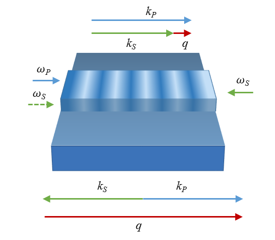
Figure 1: Schematic geometry of the interacting waves in integrated SBS. Arrows at the top denote wavenumbers for forward SBS; arrows at the bottom denote wavenumbers for backward SBS.

Following standard quantum mechanics, we naturally choose the commutation relations

$$\left[u^{n}(\mathbf{r}),\pi^{m}(\mathbf{r^{\prime}})\right]=i\hbar\delta^{nm}\delta(\mathbf{r}-\mathbf{r^{\prime}}),$$ (2)

where superscripts stand for Cartesian components. The obvious acoustic Hamiltonian operator is

$$H^{\text{A}}=\int\frac{\pi^{i}(\mathbf{r})\pi^{i}(\mathbf{r})}{2\rho(\mathbf{r})}\mathrm{d}\mathbf{r}+\frac{1}{2}\int S^{ij}(\mathbf{r})c^{ijkl}(\mathbf{r})S^{kl}(\mathbf{r})\,\mathrm{d}\mathbf{r},$$ (3)

where the integration is over all space. Here $\rho(\mathbf{r})$ and $c^{ijkl}(\mathbf{r})$ are position-dependent c-number quantities representing the density and stiffness tensor respectively, while

$$S^{ij}(\mathbf{r})=\frac{1}{2}\left(\frac{\partial u^{i}(\mathbf{r})}{\partial r^{j}}+\frac{\partial u^{j}(\mathbf{r})}{\partial r^{i}}\right),$$ (4)

is the strain tensor operator Auld (1990), and again we emphasise that unless stated otherwise, $\mathbf{u}(\mathbf{r})$ and ${\boldsymbol{\pi}}(\mathbf{r})$ are to be read as operators. In (3) and throughout, repeated indices are to be summed over the Cartesian coordinates $x,y,z$. We will formally assume these quantities are continuous functions of position, although they may change drastically as one moves from solid to air, for example. The limit to these functions changing discontinuously can be taken at the end of the calculation when matrix elements and the like are evaluated, but in all dynamical equations and derivations $\rho(\mathbf{r})$ and $c^{ijkl}(\mathbf{r})$ should be taken as continuous functions.

Let us comment on the precise meaning of the operators $\mathbf{u}$ and ${\boldsymbol{\pi}}$. In elastic theory, the displacement field applies to “volume elements” much larger than the atomic scale, but much smaller than the characteristic wavelength of any acoustic excitation. Therefore, the displacement and momentum operators do not correspond directly to any individual physical oscillator but describe collective excitations of the mesoscopic bulk medium. Nevertheless the low-energy phonon excitations that emerge from the theory are very real and their quantization is physical. For example, completeness relations are correct up to an appropriate wavevector cutoff, far above the typical wavevector of any Brillouin-induced excitation.

The strain tensor (4) is obviously symmetric in its two indices, and since the stiffness tensor appears with two strain tensors in (3), $c^{ijkl}(\mathbf{r})$ can be taken to satisfy $c^{ijkl}(\mathbf{r})=c^{ijlk}(\mathbf{r}),$ as well as $c^{ijkl}(\mathbf{r})=c^{klij}(\mathbf{r})$. In all then Landau and Lifshitz (1986) ,

$$c^{ijkl}(\mathbf{r})=c^{jikl}(\mathbf{r})=c^{ijlk}(\mathbf{r}),$$ (5)

so we can write (3) as simply

$$H^{\text{A}}=\int\frac{\pi^{i}(\mathbf{r})\pi^{i}(\mathbf{r})}{2\rho(\mathbf{r})}\,\mathrm{d}\mathbf{r}+\frac{1}{2}\int\frac{\partial u^{i}(\mathbf{r})}{\partial r^{j}}c^{ijlm}(\mathbf{r})\frac{\partial u^{l}(\mathbf{r})}{\partial r^{m}}\,\mathrm{d}\mathbf{r}.$$ (6)

Evaluating the Heisenberg equations of motion (see supplementary material section S.I)

$$i\hbar\frac{\partial}{\partial t}u^{n}(\mathbf{r},t) = \left[u^{n}(\mathbf{r}),H^{\text{A}}\right],$$ (7a)

$$i\hbar\frac{\partial}{\partial t}\pi^{n}(\mathbf{r},t) = \left[\pi^{n}(\mathbf{r}),H^{\text{A}}\right],$$ (7b)

yields

$$\frac{\partial}{\partial t}u^{n}(\mathbf{r},t) = \frac{\pi^{n}(\mathbf{r},t)}{\rho(\mathbf{r})},$$ (8a)

$$\frac{\partial}{\partial t}\pi^{n}(\mathbf{r},t) = \frac{\partial}{\partial r^{j}}\bigg{(}c^{njkl}(\mathbf{r})S^{kl}(\mathbf{r})\bigg{)}.$$ (8b)

Classically these equations indicate, as expected, that the conjugate momentum is the product of the mass density and the velocity field $\dot{u}^{n}$, and that the momentum evolves according to Newton’s laws.

From (8), we recover the standard acoustic wave equation Auld (1990):

$$\rho(\mathbf{r})\frac{\partial^{2}u^{n}(\mathbf{r},t)}{\partial t^{2}}=\frac{\partial}{\partial r^{j}}\bigg{(}c^{njkl}(\mathbf{r})S^{kl}(\mathbf{r})\bigg{)}.$$ (9)

Thus we have the desired equations of motion in both the classical and quantum descriptions. Moreover, substituting the relation (8a) into (3) and taking the classical limit by dropping the operator nature of $\mathbf{u}$ and $S^{ij}$, we recover the classical Hamiltonian

$$H^{\text{A}} \rightarrow \frac{1}{2}\int\rho(\mathbf{r})\left(\frac{\partial\mathbf{u}(\mathbf{r},t)}{\partial t}\right)^{2}\mathrm{d}\mathbf{r}+\frac{1}{2}\int S^{ij}(\mathbf{r})c^{ijkl}(\mathbf{r})S^{kl}(\mathbf{r})\,\mathrm{d}\mathbf{r}$$

$$= T+V.$$

This is clearly numerically equal to the sum of kinetic and potential energy Auld (1990), and so (3) meets all the criteria to be an appropriate Hamiltonian for quantization. Note that at this point, no acoustic dissipation (viscosity) has been included. Direct incorporation of losses is less straightforward in Hamiltonian approaches than in Lagrangian approaches, in which a Rayleigh dissipation function can be introduced. The phonon loss is important to the physics of SBS, but can be incorporated later perturbatively. We discuss this in Section VI.

II.2 Modes and new fields

We now seek to reduce the Hamiltonian to standard harmonic oscillator form; the low energy states will describe the quasi-particle or phonon excitations of the medium. To diagonalise the acoustic Hamiltonian we look for classical solutions of (9) of the form

$$\mathbf{u}(\mathbf{r},t)=\mathbf{U}_{\Lambda}(\mathbf{r})\mathrm{e}^{-i\Omega_{\Lambda}t}+\text{c.c.},$$ (10)

where $\Lambda$ is a mode index. This implies

$$-\frac{\partial}{\partial r^{j}}\left(c^{njkl}(\mathbf{r})\frac{\partial U_{\Lambda}^{k}(\mathbf{r)}}{\partial r^{l}}\right)=\rho(\mathbf{r})\Omega_{\Lambda}^{2}U_{\Lambda}^{n}(\mathbf{r}),$$ (11)

where again we have used the fact that $c^{njkl}(\mathbf{r})$ is symmetric in its last two indices. It is convenient however, if the linear operator generating mode functions is Hermitian, which the form in Eq. (11) is not. To obtain a Hermitian system, we introduce new fields

$$\tilde{\mathbf{u}}(\mathbf{r}) = \sqrt{\rho(\mathbf{r})}\,\mathbf{u}(\mathbf{r})$$ (12)

$$\tilde{{\boldsymbol{\pi}}}(\mathbf{r}) = \frac{{\boldsymbol{\pi}}(\mathbf{r})}{\sqrt{\rho(\mathbf{r})}},$$

which clearly preserve the commutation relations. That is,

$$\left[\tilde{u}^{n}(\mathbf{r}),\tilde{\pi}^{m}(\mathbf{r^{\prime}})\right]=i\hbar\delta^{nm}\delta(\mathbf{r}-\mathbf{r^{\prime}}).$$ (13)

We now look for mode solutions in terms of the new fields in the form

$$\tilde{\mathbf{u}}(\mathbf{r},t) = \mathbf{\tilde{U}}_{\Lambda}(\mathbf{r})\mathrm{e}^{-i\Omega_{\Lambda}t}+\text{c.c.},$$ (14a)

$$\tilde{{\boldsymbol{\pi}}}(\mathbf{r},t) = \mathbf{\tilde{\Pi}}_{\Lambda}(\mathbf{r})\mathrm{e}^{-i\Omega_{\Lambda}t}+\text{c.c.}$$ (14b)

We introduce the operator $\mathcal{M}^{nk}$ which acts on a general vector function $\mathbf{C}(\mathbf{r})$ as

$$\mathcal{M}^{nk}(\mathbf{r})C^{k}(\mathbf{r})=-\frac{1}{\sqrt{\rho(\mathbf{r})}}\frac{\partial}{\partial r^{j}}\left(c^{njkl}(\mathbf{r})\frac{\partial}{\partial r^{l}}\left(\frac{C^{k}(\mathbf{r})}{\sqrt{\rho(\mathbf{r})}}\right)\right).$$ (15)

Section S.II of the supplementary material shows that $\mathcal{M}^{nk}(\mathbf{r})$ is indeed Hermitian. Then, using integration by parts we can write the Hamiltonian (3) in terms of the new fields (12) in the simple form

$$H^{\text{A}} = \frac{1}{2}\int\tilde{\pi}^{i}(\mathbf{r})\tilde{\pi}^{i}(\mathbf{r})\,\mathrm{d}\mathbf{r}+\frac{1}{2}\int\tilde{u}^{i}(\mathbf{r})\mathcal{M}^{ik}(\mathbf{r})\tilde{u}^{k}(\mathbf{r})\,\mathrm{d}\mathbf{r}.$$ (16)

As the basis of our acoustic modal expansion, Eq. (15) plays an analogous role to that which the vector Helmholtz equation (commonly known as the “master equation” in the photonic crystal literature Joannopoulos et al. (2008),) plays in the quantization of the electromagnetic field (see (43) below). Its Hermitian form is useful both for developing the formalism but also for formulating mode-solving algorithms based on energy functional minimization Joannopoulos et al. (2008).

Now if we construct eigenfunctions $\mathbf{F}_{\Lambda}(\mathbf{r})$ of $\mathcal{M}^{nk}$ such that

$$\mathcal{M}^{nk}(\mathbf{r})F_{\Lambda}^{k}(\mathbf{r})=\Omega_{\Lambda}^{2}F_{\Lambda}^{n}(\mathbf{r}),$$ (17)

it follows from (11) and (12) that we can take

$$\mathbf{\tilde{U}}_{\Lambda}(\mathbf{r}) = \mathbf{F}_{\Lambda}(\mathbf{r}),$$ (18)

$$\mathbf{\tilde{\Pi}}_{\Lambda}(\mathbf{r}) = -i\Omega_{\Lambda}\mathbf{F}_{\Lambda}(\mathbf{r}),$$

where the second equation follows from substituting (14) in (8a).

From the Hermiticity of $\mathcal{M}^{nk}$, the eigenfunctions $\mathbf{F}_{\Lambda}(\mathbf{r})$ with different eigenvalues will automatically be orthogonal, and if there are eigenfunctions with the same eigenvalue we can construct them to be orthogonal. Thus we can write

$$\int\mathbf{F}_{\Lambda}^{*}(\mathbf{r})\cdot\mathbf{F}_{\Lambda^{\prime}}(\mathbf{r})\,\mathrm{d}\mathbf{r}=\delta_{\Lambda\Lambda^{\prime}}.$$ (19)

Here the integration is over a finite volume that, in the end, can be allowed to pass to infinity if we wish to generate a continuum of eigenfunctions. We take the set of eigenfunctions with positive eigenvalues $\Omega_{\Lambda}^{2}$ as complete,

$$\sum_{\Lambda}F_{\Lambda}^{n}(\mathbf{r})\left(F_{\Lambda}^{m}(\mathbf{r}^{\prime})\right)^{*}=\delta^{nm}\delta(\mathbf{r}-\mathbf{r^{\prime}}),$$ (20)

at least for the problems of interest. For each $\Omega_{\Lambda}^{2}$ we choose a positive $\Omega_{\Lambda}$ and take it as the frequency of the eigenfunction. Some additional properties of the mode functions that are required for reduction of the acoustic Hamiltonian to canonical harmonic oscillator form are developed in section S.III of the supplementary material.

Following similar arguments to those used in quantization of the vacuum electromagnetic field Grynberg et al. (2010) (or the electromagnetic field in nondispersive media Sipe et al. (2004)), one can show using (20) that introducing new operators $b_{\Lambda}$ and $b^{\dagger}_{\Lambda}$ with commutation relations

$$\left[b_{\Lambda},b_{\Lambda^{\prime}}\right] = 0,$$ (21)

$$\left[b_{\Lambda},b_{\Lambda^{\prime}}^{\dagger}\right] = \delta_{\Lambda\Lambda^{\prime}},$$

we can preserve the commutation relations (13), by expanding the fields as

$$\mathbf{\tilde{u}(r}) =\sum_{\Lambda}\sqrt{\frac{\hbar}{2\Omega_{\Lambda}}}b_{\Lambda}\mathbf{F}_{\Lambda}(\mathbf{r})+\text{h.c.},$$ (22a)

$$\tilde{{\boldsymbol{\pi}}}(\mathbf{r}) =-i\sum_{\Lambda}\sqrt{\frac{\hbar\Omega_{\Lambda}}{2}}b_{\Lambda}\mathbf{F}_{\Lambda}(\mathbf{r})+\text{h.c.},$$ (22b)

where h.c. is the Hermitian conjugate. Then, through a series of manipulations using properties of the $F_{\Lambda}(\mathbf{r})$, the Hamiltonian can be reduced to the canonical harmonic oscillator form

$$H^{\text{A}} = \sum_{\Lambda}\hbar\Omega_{\Lambda}b_{\Lambda}^{\dagger}b_{\Lambda},$$ (23)

where we have dropped the zero point energy which has no dynamical effect. Derivations of Eqs. (22) and (23) are provided in section S.IV of the supplementary material.

Finally, returning to the physical modes by introducing

$$\mathbf{U}_{\Lambda}(\mathbf{r}) =\frac{1}{\Omega_{\Lambda}\sqrt{\rho(\mathbf{r})}}\mathbf{F}_{\Lambda}(\mathbf{r}),$$ (24a)

$$\mathbf{\Pi}_{\Lambda}(\mathbf{r}) =-i\sqrt{\rho(\mathbf{r})}\mathbf{F}_{\Lambda}(\mathbf{r}),$$ (24b)

we can write the full displacement and momentum field operators as

$$\mathbf{u}(\mathbf{r}) = \sum_{\Lambda}\sqrt{\frac{\hbar\Omega_{\Lambda}}{2}}b_{\Lambda}\mathbf{U}_{\Lambda}(\mathbf{r})+\text{h.c.},$$ (25a)

$${\boldsymbol{\pi}}(\mathbf{r}) = \sum_{\Lambda}\sqrt{\frac{\hbar\Omega_{\Lambda}}{2}}b_{\Lambda}\mathbf{\Pi}_{\Lambda}(\mathbf{r})+\text{h.c.},$$ (25b)

with prefactors in the expansions reminiscent of simple harmonic oscillator physics.

II.3 Waveguide acoustics

The results to this point apply to any acoustic structure. We now specialize to waveguides running along the $z$ direction, and choose a box of length $L$ in that direction, which includes all $x$ and $y$. Focusing on acoustic modes confined to the waveguide, we label the modes by a wavenumber $q=2\pi n/L$, for integer $n$, and a band $\alpha$ which identifies the transverse spatial mode structure in the $xy$ plane. Then the eigenfunctions of the previous section can be written

$$\mathbf{F}_{\alpha q}(\mathbf{r})=\frac{\mathbf{f}_{\alpha q}(x,y)\mathrm{e}^{iqz}}{\sqrt{L}},$$ (26)

with the normalization (19) guaranteed by requiring

$$\int\mathrm{d}x\mathrm{d}y\,\mathbf{f}_{\alpha q}^{*}(x,y)\cdot\mathbf{f}_{\alpha q}(x,y)=1,$$ (27)

where the integration is over the whole $x$-$y$ plane. The derived mode amplitudes (24) are then of the form

$$\mathbf{U}_{\alpha q}(\mathbf{r}) = \frac{\mathbf{u}_{\alpha q}(x,y)\mathrm{e}^{iqz}}{\sqrt{L}},$$

$$\mathbf{\Pi}_{\alpha q}(\mathbf{r}) = \frac{{\boldsymbol{\pi}}_{\alpha q}(x,y)\mathrm{e}^{iqz}}{\sqrt{L}},$$

with

$$\mathbf{u}_{\alpha q}(x,y) =\frac{1}{{\Omega_{\alpha q}}\sqrt{\rho(x,y)}}\,\mathbf{f}_{\alpha q}(x,y),$$ (28a)

$${\boldsymbol{\pi}}_{\alpha q}(x,y) =-i\sqrt{\rho(x,y)}\,\mathbf{f}_{\alpha q}(x,y).$$ (28b)

Note that the normalization condition (27) can be written, using (28a), as

$$\Omega^{2}_{\alpha q}\int\mathrm{d}x\mathrm{d}y\,\rho(x,y)\,\mathbf{u}_{\alpha q}^{*}(x,y)\cdot\mathbf{u}_{\alpha q}(x,y)=1.$$ (29)

If we now let $L\rightarrow\infty$, moving to a continuous distribution of modes, the commutation relations, Hamiltonian and field operator expansions respectively become

$$\left[b_{\alpha q},b_{\alpha^{\prime}q^{\prime}}\right] = 0,$$

$$\left[b_{\alpha q},b_{\alpha^{\prime}q^{\prime}}^{\dagger}\right] = \delta_{\alpha\alpha^{\prime}}\delta(q-q^{\prime}),$$

$$H^{\text{A}}=\sum_{\alpha}\int\mathrm{d}q\,\hbar{\Omega_{\alpha q}}b_{\alpha q}^{{\dagger}}b_{\alpha q},$$ (30)

$$\mathbf{u}(\mathbf{r}) = \sum_{\alpha}\int\frac{\mathrm{d}q}{\sqrt{2\pi}}\sqrt{\frac{\hbar{\Omega_{\alpha q}}}{2}}b_{\alpha q}(t)\mathbf{u}_{\alpha q}(x,y)\,\mathrm{e}^{iqz}+\text{h.c.},$$ (31)

$${\boldsymbol{\pi}}(\mathbf{r}) = \sum_{\alpha}\int\frac{\mathrm{d}q}{\sqrt{2\pi}}\sqrt{\frac{\hbar{\Omega_{\alpha q}}}{2}}b_{\alpha q}(t){\boldsymbol{\pi}}_{\alpha q}(x,y)\,\mathrm{e}^{iqz}+\text{h.c.},$$

while (27)–(29) remain unchanged. Here the $q$ integrals are over the range of $q$ for which each mode $\alpha$ exists, taking account of any modal cutoffs. Normally we work in the Heisenberg regime so the $b_{\alpha q}$ are time-dependent. Note our convention that while $\mathbf{u}$ and ${\boldsymbol{\pi}}$ are operators, the mode functions $\mathbf{u}_{\alpha q}$ and ${\boldsymbol{\pi}}_{\alpha q}$, which carry modal index subscripts, are c-number quantities.

II.4 Envelope functions

To make the connection to the more familiar waveguide representation of slowly-varying envelopes, we now introduce envelope functions for each type of acoustic mode. We assume the excitation is centered at some wavenumber $q_{\text{\tiny o}}$ and factor out that dependence to produce a function varying slowly in space. However we retain the full time-dependence in the operators $b_{\alpha q}(t)$ writing

$$\phi_{\alpha}(z,t)=\int\frac{\mathrm{d}q}{\sqrt{2\pi}}b_{\alpha q}(t)\mathrm{e}^{i(q-q_{\text{\tiny o}})z}.$$ (32)

If the integral in (32) is taken to range over all $q$ it is easily checked that we obtain the canonical equal-time continuous commutators

$$\left[\phi_{\alpha}(z,t),\phi_{\alpha^{\prime}}^{\dagger}(z^{\prime},t)\right]=\delta_{\alpha\alpha^{\prime}}\delta(z-z^{\prime}).$$ (33)

In reality, the range of integration in (32) is restricted by modal cutoffs, which will temper the Dirac delta function in (33). However, assuming spectrally narrow envelopes far from any cut-offs, Eq. (33) should normally be an excellent approximation. From (31) we see that if $\Omega_{\alpha q}$, $\mathbf{u}_{\alpha q}(x,y)$, and ${\boldsymbol{\pi}}_{\alpha q}(x,y)$ vary little over the range of significant $q$ we can approximate the field expansions in terms of envelope functions centered at $q=q_{\text{\tiny o}}$:

$$\mathbf{u}(\mathbf{r}) \simeq \sum_{\alpha q_{\text{\tiny o}}}\mathrm{e}^{iq_{\text{\tiny o}}z}\sqrt{\frac{\hbar\Omega_{\alpha q_{\text{\tiny o}}}}{2}}\mathbf{u}_{\alpha q_{\text{\tiny o}}}(x,y)\int\frac{\mathrm{d}q}{\sqrt{2\pi}}b_{\alpha q}(t)\mathrm{e}^{i(q-q_{\text{\tiny o}})z}+\text{h.c.},$$

$$= \sum_{\alpha q_{\text{\tiny o}}}\mathrm{e}^{iq_{\text{\tiny o}}z}\sqrt{\frac{\hbar\Omega_{\alpha q_{\text{\tiny o}}}}{2}}\mathbf{u}_{\alpha q_{\text{\tiny o}}}(x,y)\,\phi_{\alpha}(z,t)+\text{h.c.},$$

$${\boldsymbol{\pi}}(\mathbf{r}) \simeq \sum_{\alpha q_{\text{\tiny o}}}\mathrm{e}^{iq_{\text{\tiny o}}z}\sqrt{\frac{\hbar\Omega_{\alpha q_{\text{\tiny o}}}}{2}}{\boldsymbol{\pi}}_{\alpha q_{\text{\tiny o}}}(x,y)\int\frac{\mathrm{d}q}{\sqrt{2\pi}}b_{\alpha q}(t)\mathrm{e}^{i(q-q_{\text{\tiny o}})z}+\text{h.c.}$$

$$= \sum_{\alpha q_{\text{\tiny o}}}\mathrm{e}^{iq_{\text{\tiny o}}z}\sqrt{\frac{\hbar\Omega_{\alpha q_{\text{\tiny o}}}}{2}}{\boldsymbol{\pi}}_{\alpha q_{\text{\tiny o}}}(x,y)\,\phi_{\alpha}(z,t)+\text{h.c.}.$$

Corrections can be included by expanding the prefactors $\sqrt{\hbar\Omega_{\alpha q}/2}\,\mathbf{u}_{\alpha q}(x,y)$ and $\sqrt{\hbar\Omega_{\alpha q}/2}\,{\boldsymbol{\pi}}_{\alpha q}(x,y)$ about $q=q_{o}$, and combining the resulting powers of $(q-q_{o})$ with the $\exp(i(q-q_{o})z)$ in the integrals over $q$ to yield expressions involving derivatives of $\phi_{\alpha}(z,t)$, but we neglect them here.

Returning to Eq. (32), we can derive approximate equations of motion for the $\phi_{\alpha}(z,t)$ in the Heisenberg picture by expanding the dispersion relation ${\Omega_{\alpha q}}$ of mode $\alpha$ about $q_{\text{\tiny o}}$:

$$\frac{\partial\phi_{\alpha}}{\partial t} =\frac{1}{i\hbar}[\phi_{\alpha},H^{\text{A}}]$$

$$=\frac{1}{i\hbar}\int\frac{\mathrm{d}q}{\sqrt{2\pi}}\hbar\Omega_{q}\mathrm{e}^{i(q-q_{\text{\tiny o}})z}b_{\alpha q}(t)$$

$$=-i\int\frac{\mathrm{d}q}{\sqrt{2\pi}}\left(\Omega_{\alpha q_{0}}+v_{\alpha q_{\text{\tiny o}}}(q-q_{0})+\frac{1}{2}v_{\alpha q_{\text{\tiny o}}}^{\prime}(q-q_{0})^{2}+\ldots\right)\mathrm{e}^{i(q-q_{\text{\tiny o}})z}b_{\alpha q}(t)$$

$$\approx-i\Omega_{\alpha q_{0}}\phi_{\alpha}(z,t)-v_{\alpha q_{\text{\tiny o}}}\frac{\partial\phi_{\alpha}(z,t)}{\partial z}+\frac{1}{2}iv_{\alpha q_{\text{\tiny o}}}^{\prime}\frac{\partial^{2}\phi_{\alpha}(z,t)}{\partial t^{2}}+\ldots,$$ (34)

where

$$v_{\alpha q_{\text{\tiny o}}} = \left(\frac{\mathrm{d}{\Omega_{\alpha q}}}{\mathrm{d}q}\right)_{q=q_{\text{\tiny o}}},$$ (35a)

$$v_{\alpha q_{\text{\tiny o}}}^{\prime} = \left(\frac{\mathrm{d}^{2}{\Omega_{\alpha q}}}{\mathrm{d}q^{2}}\right)_{q=q_{\text{\tiny o}}},$$ (35b)

etc. An expression for the group velocity $v_{\alpha q}$ in terms of the modal fields is worked out in section S.V of the supplementary material.

II.5 Acoustic powers

Finally, we establish some expressions concerning the power carried by the acoustic modes in the envelope representation. Classically, the acoustic power density at a point in the medium in a direction $\hat{\mathbf{n}}$ is given by

$${\cal P}^{\text{A}}_{\text{cl}}\cdot\hat{\mathbf{n}}=-\frac{\partial u^{i}(\mathbf{r})}{\partial t}c^{ijkl}(\mathbf{r})S^{kl}(\mathbf{r})n^{j},$$ (36)

which has the natural interpretation of power being the dot product of an applied force and the velocity of the point of application Auld (1990). Using (8), the power carried by a waveguide mode in the $\hat{\mathbf{z}}$ direction is thus

$$P^{\text{A}}_{\text{cl}}(z)=-\int\mathrm{d}x\mathrm{d}y\,\frac{\pi^{i}(\mathbf{r})}{\rho(x,y)}c^{izkl}(x,y)S^{kl}(\mathbf{r}).$$ (37)

To construct a quantum operator corresponding to the power density we use the symmetrized form of the non-commuting operators ${\boldsymbol{\pi}}(\mathbf{r})$ and $S^{kl}(\mathbf{r})$, in the usual way, as shown in section S.VI of the supplementary material. This leads to the result that the operator for the power carried by the acoustic field is

$$P^{\text{A}}(z)=\sum_{\alpha,\alpha^{\prime}}\int\frac{\mathrm{d}q\mathrm{d}q^{\prime}}{2\pi}b_{\alpha^{\prime}q^{\prime}}^{\dagger}(t)b_{\alpha q}(t)\mathrm{e}^{i(q-q^{\prime})z}p^{\text{A}}_{\alpha^{\prime}\alpha}(q^{\prime},q).$$ (38)

Here the contribution from the pair of modes $\alpha$ and $\alpha^{\prime}$ at wavenumbers $q^{\prime}$ and $q$ is given by

$$p^{\text{A}}_{\alpha^{\prime}\alpha}(q^{\prime},q) = \frac{\hbar}{2}\sqrt{\frac{\Omega_{\alpha^{\prime}q^{\prime}}}{{\Omega_{\alpha q}}}}q\int\mathrm{d}x\mathrm{d}y\,\frac{c^{izkz}(x,y)}{\rho(x,y)}\left(f_{\alpha^{\prime}q^{\prime}}^{i}(x,y)\right)^{*}f_{\alpha q}^{k}(x,y)$$

$$+\frac{\hbar}{2}\sqrt{\frac{{\Omega_{\alpha q}}}{\Omega_{\alpha^{\prime}q^{\prime}}}}q^{\prime}\int\mathrm{d}x\mathrm{d}y\,\frac{c^{izkz}(x,y)}{\rho(x,y)}\left(f_{\alpha^{\prime}q^{\prime}}^{k}(x,y)\right)^{*}\left(f_{\alpha q}^{i}(x,y)\right)$$

$$-\frac{i\hbar}{2}\sqrt{\frac{\Omega_{\alpha^{\prime}q^{\prime}}}{{\Omega_{\alpha q}}}}\int\mathrm{d}x\mathrm{d}y\,\frac{\left(f_{\alpha^{\prime}q^{\prime}}^{i}(x,y)\right)^{*}}{\sqrt{\rho(x,y)}}c^{izkl}(x,y)\left(\frac{\partial}{\partial r^{l}}\left(\frac{f_{\alpha q}^{k}(x,y)}{\sqrt{\rho(x,y)}}\right)\right)$$

$$+\frac{i\hbar}{2}\sqrt{\frac{{\Omega_{\alpha q}}}{\Omega_{\alpha^{\prime}q^{\prime}}}}\int\mathrm{d}x\mathrm{d}y\,\frac{\left(f_{\alpha q}^{i}(x,y)\right)}{\sqrt{\rho(x,y)}}c^{izkl}(x,y)\left(\frac{\partial}{\partial r^{l}}\left(\frac{f_{\alpha^{\prime}q^{\prime}}^{k}(x,y)}{\sqrt{\rho(x,y)}}\right)\right)^{*},$$

where we have used (II.3) to introduce the modified mode functions $\mathbf{f}_{\alpha,q}$.

For a phonon field involving only one mode $\alpha$ and assuming we can neglect the $q$ dependence of $p_{\alpha\alpha}(q,q^{\prime})$ over the pulse spectrum we obtain the slowly-varying power operator as

$$P^{\text{A}}_{\text{sv}}(z) \simeq \int\frac{\mathrm{d}q\mathrm{d}q^{\prime}}{2\pi}b_{\alpha q^{\prime}}^{\dagger}(t)b_{\alpha q}(t)\mathrm{e}^{i(q-q^{\prime})z}p^{\text{A}}_{\alpha\alpha}(q_{\text{\tiny o}},q_{\text{\tiny o}})$$

$$= p^{\text{A}}_{\alpha\alpha}(q_{\text{\tiny o}},q_{\text{\tiny o}})\phi_{\alpha}^{\dagger}(z)\phi_{\alpha}(z).$$

Finally, it may be shown (see section S.VI of the supplementary material), that $p^{\text{A}}_{\alpha\alpha}(q_{\text{\tiny o}},q_{\text{\tiny o}})=\hbar\Omega_{\alpha q_{\text{\tiny o}}}v_{\alpha q_{\text{\tiny o}}}$, so that the power carried by the acoustic envelope is

$$P^{\text{A}}_{\text{sv}}(z)=\hbar\Omega_{\alpha q_{\text{\tiny o}}}\,v_{\alpha q_{\text{\tiny o}}}\,\phi_{\alpha}^{\dagger}(z)\phi_{\alpha}(z),$$ (40)

and it follows that in this limit, $\phi_{\alpha}^{\dagger}(z)\phi_{\alpha}(z)$ has the natural interpretation of a phonon number density operator.

III Quantization of the electromagnetic fields

To construct the full opto-acoustic Hamiltonian we will need similar results for the quantization of the electromagnetic field in integrated structures. The procedure is well known and we simply summarize some essential results Sipe et al. (2004).

III.1 Hamiltonian and modes

As the fundamental quantum fields we take the electric displacement $\mathbf{D}\left(\mathbf{r}\right)$ and magnetic $\mathbf{B}\left(\mathbf{r}\right)$ fields with commutation relations

$$\left[D^{i}(\mathbf{r}),D^{j}(\mathbf{r^{\prime}})\right] = \left[B^{i}(\mathbf{r}),B^{j}(\mathbf{r^{\prime}})\right]=0,$$

$$\left[D^{i}(\mathbf{r}),B^{j}(\mathbf{r^{\prime}})\right] = i\hbar\epsilon^{ilj}\frac{\partial}{\partial r^{l}}\delta(\mathbf{r}-\mathbf{r^{\prime}}).$$

This choice, which dates back to Born and Infeld Born and Infeld (1934) has the advantage that the transversality of the two fields is easily imposed. The quantization procedure has been discussed at length elsewhere Sipe et al. (2004), and we simply quote the necessary. The parallels to the acoustic problem in the previous section are very apparent.

The electromagnetic Hamiltonian operator is taken as

$$H^{\text{EM}}=\frac{1}{2\mu_{0}}\int B^{i}(\mathbf{r})B^{i}(\mathbf{r})\,\mathrm{d}\mathbf{r}+\frac{1}{2\epsilon_{0}}\int D^{i}(\mathbf{r})\beta_{\text{ref}}(\mathbf{r})D^{i}(\mathbf{r})\,\mathrm{d}\mathbf{r},$$ (41)

where

$$\beta_{\text{ref}}(\mathbf{r})=\frac{1}{\epsilon_{\text{ref}}(\mathbf{r})},$$ (42)

describes the “background” dielectric response of the waveguide structure in terms of the relative dielectric constant $\epsilon_{\text{ref}}(\mathbf{r})$, without any acoustic effects. Note that it is straightforward to include a tensor response in $\epsilon_{\text{ref}}(\mathbf{r})$ but to reduce cluttering the tensor notation, here we treat the material as optically isotropic. In principle, we could also extend the treatment to include dispersion of the dielectric Bhat and Sipe (2006) at the expense of considerably more complexity. For Brillouin processes, the linewidths of the interacting optical waves are usually narrow, and we can safely neglect dispersion within each optical field.

As with the acoustic case, we are interested in optical waveguide modes with translational invariance along $z$. We find these modes $\{\mathbf{B}_{\Lambda}(\mathbf{r}),\omega_{\Lambda}\}$ by solution of the vector Helmholtz equation

$$\nabla\times\big{[}\beta_{\text{ref}}(x,y)\nabla\times\mathbf{B}_{\Lambda}\big{]}=\frac{\omega_{\Lambda}^{2}}{c^{2}}\mathbf{B},$$ (43)

together with Ampere’s law

$$\mathbf{D}_{\Lambda}(\mathbf{r})=\frac{i}{\mu_{0}\omega_{\Lambda}}\nabla\times\mathbf{B}_{\Lambda},$$ (44)

and then introduce waveguide mode functions $\mathbf{d}_{\gamma k}$ defined by

$$\mathbf{D}_{\gamma k}(\mathbf{r})=\frac{\mathbf{d}_{\gamma k}(x,y)}{\sqrt{2\pi}}\mathrm{e}^{ikz},$$ (45)

where $\gamma$ indexes the transverse spatial bands of the waveguide. We choose the normalization

$$\frac{1}{\epsilon_{0}}\int\mathrm{d}x\mathrm{d}y\,\beta_{\text{ref}}(\mathbf{r})\,\mathbf{d}_{\gamma k}^{*}(x,y)\cdot\mathbf{d}_{\gamma k}(x,y) = 1,$$ (46)

and expand the displacement field operator as

$$\mathbf{D}(\mathbf{r}) = \sum_{\gamma}\int\frac{\mathrm{d}k}{\sqrt{2\pi}}\sqrt{\frac{\hbar\omega_{\gamma k}}{2}}a_{\gamma k}\mathbf{d}_{\gamma k}(x,y)\mathrm{e}^{ikz}+\text{h.c.}.$$ (47)

The mode operators $a_{\gamma k}$ satisfy the standard commutation relations

$$\left[a_{\gamma k},a_{\gamma{{}^{\prime}}k^{\prime}}\right] =0,$$

$$\left[a_{\gamma k},a_{\gamma{{}^{\prime}}k^{\prime}}^{\dagger}\right] =\delta_{\gamma\gamma{{}^{\prime}}}\delta(k-k^{\prime}),$$

and neglecting the vacuum energy, the electromagnetic Hamiltonian reduces to

$$H^{\text{EM}}=\sum_{\gamma}\int\mathrm{d}k\,\hbar\omega_{\gamma k}\,a_{\gamma k}^{\dagger}a_{\gamma k}.$$ (48)

III.2 Envelope operators

As with the acoustic modes we can introduce envelope function operators associated with a mode $\gamma$ and a range of wavenumbers in the neighborhood of some $k_{j}$:

$$\psi_{\gamma j}(z)=\int\frac{\mathrm{d}k}{\sqrt{2\pi}}a_{\gamma k}(t)\mathrm{e}^{i(k-k_{j})z}.$$ (49)

The integration is to be taken over the range of wavenumbers $k$ that we wish to associate with the center value $k_{j}$. This allows the introduction of distinct envelope operators for fields that occupy the same spatial mode but occupy distinct frequency ranges (such as a pump and Stokes wave in the same mode).

If the integrals in (49) were to extend over all $k$ we would obtain

$$\left[\psi_{\gamma j}(z,t),\psi_{\gamma{{}^{\prime}}j^{\prime}}^{{\dagger}}(z^{\prime},t)\right]=\delta_{\gamma\gamma{{}^{\prime}}}\delta_{jj^{\prime}}\delta(z-z^{\prime}).$$ (50)

In principle, the existence of cutoffs and the possible partitioning of each channel $\gamma$ into separate bands for pump and Stokes waves means that the $k$ integrals have restricted range, but as with the acoustic fields, we assume the excitations are sufficiently narrow band and away from cutoff that the integrals leading to the Dirac delta function in (50) can be safely extended to infinity. Assuming in fact that only values of $k$ close to $k_{j}$ are important for each mode $\gamma j$, as we now label them, we can write

$$\mathbf{D}(\mathbf{r}) = \sum_{\gamma}\int\frac{\mathrm{d}k}{\sqrt{2\pi}}\,\sqrt{\frac{\hbar\omega_{\gamma k}}{2}}a_{\gamma k}(t)\mathbf{d}_{\gamma k}(x,y)\mathrm{e}^{ikz}+\text{h.c.}$$

$$= \sum_{\gamma,j}\mathrm{e}^{ik_{j}z}\int\frac{\mathrm{d}k}{\sqrt{2\pi}}\,\sqrt{\frac{\hbar\omega_{\gamma k}}{2}}a_{\gamma k}(t)\mathbf{d}_{\gamma k}(x,y)\mathrm{e}^{i(k-k_{j})z}+\text{h.c.}$$

$$\approx \sum_{\gamma,j}\mathrm{e}^{ik_{j}z}\sqrt{\frac{\hbar\omega_{\gamma}^{j}}{2}}\mathbf{d}_{\gamma k_{j}}(x,y)\int\frac{\mathrm{d}k}{\sqrt{2\pi}}\;a_{\gamma k}(t)\mathrm{e}^{i(k-k_{j})z}+\text{h.c.}$$

$$= \sum_{\gamma,j}\mathrm{e}^{ik_{j}z}\sqrt{\frac{\hbar\omega_{\gamma}^{j}}{2}}\mathbf{d}_{\gamma k_{j}}(x,y)\,\psi_{\gamma j}(z)+\text{h.c.},$$

where we have put $\omega_{\gamma}^{j}\equiv\omega_{\gamma k_{j}}$ and neglected the variation in $\sqrt{\omega_{\gamma}^{j}}$ and the $k$ dependence of $\mathbf{d}_{\gamma k}(x,y)$; as in our treatment of acoustic fields, corrections to these expressions can be easily identified.

Again in analogy with the treatment of the acoustic fields, an operator for the slowly-varying part of the power in the waveguide can be constructed from the Poynting vector (section S.VII of the supplementary material) which takes the form

$$P^{\text{EM}}_{\text{sv}}(z)=\sum_{\gamma,\gamma{{}^{\prime}}}\int\frac{\mathrm{d}k\mathrm{d}k^{\prime}}{2\pi}a_{\gamma{{}^{\prime}}k^{\prime}}^{\dagger}(t)a_{\gamma k}(t)\mathrm{e}^{i(k-k^{\prime})z}p^{\text{EM}}_{\gamma{{}^{\prime}}\gamma}(k^{\prime},k).$$ (52)

For ranges of $k$ and $k^{\prime}$ close enough to $k_{j}$, and assuming that for different $\gamma$ the corresponding $k_{j}$ ranges are distinct, we can write this as

$$P^{\text{EM}}_{\text{sv}}(z)\approx\sum_{\gamma,j}\int\frac{\mathrm{d}k\mathrm{d}k^{\prime}}{2\pi}a_{\gamma k^{\prime}}^{\dagger}(t)a_{\gamma k}(t)\mathrm{e}^{i(k-k^{\prime})z}p^{\text{EM}}_{\gamma\gamma}(k_{j},k_{j}),$$ (53)

and since we find that

$$p^{\text{EM}}_{\gamma\gamma}(k_{j},k_{j})=\hbar\omega_{\gamma}^{j}v_{\gamma}^{j},$$ (54)

where $v_{\gamma}^{j}$ is the group velocity of electromagnetic mode type $\gamma$ centered at $k_{j}$, we have

$$P^{\text{EM}}_{\text{sv}}(z,t)\approx\sum_{\gamma,j}\hbar\omega_{\gamma}^{j}v_{\gamma}^{j}\;\psi_{\gamma j}^{\dagger}(z,t)\psi_{\gamma j}(z,t),$$ (55)

so that $\psi_{\gamma j}^{\dagger}(z,t)\psi_{\gamma j}(z,t)$ behaves as a photon number density operator; note again the similarity with the treatment of the acoustic field, for which (40) is the corresponding result. The form in Eqs. (54) and (55) does not seem to have been presented earlier, and is derived in section S.VII of the supplementary material.

Finally, in similar fashion to Eqs. (34), we find that the envelope operator obeys the dynamical equation

$$\frac{\partial\psi_{\gamma k_{j}}(z)}{\partial t} = -i\omega_{\gamma}^{j}\psi_{\gamma j}(z)-v_{\gamma}^{j}\frac{\partial\psi_{\gamma j}(z)}{\partial z}+\frac{1}{2}iv_{\gamma}^{j\prime}\frac{\partial^{2}\psi_{\gamma j}(z)}{\partial z^{2}}+\ldots$$ (56)

where

$$v_{\gamma}^{j} = \left(\frac{\mathrm{d}\omega_{\gamma k}}{\mathrm{d}k}\right)_{k=k_{j}},$$

$$v_{\gamma}^{j\prime} = \left(\frac{\mathrm{d}^{2}\omega_{\gamma k}}{\mathrm{d}k^{2}}\right)_{k=k_{j}}$$

are respectively the group velocity and group velocity dispersion of mode $\gamma j$ at its reference wavenumber $k_{j}$. For the narrow bandwidths involved in SBS physics, higher dispersive terms are unlikely to be needed.

IV The complete opto-acoustic Hamiltonian

At last, we can now assemble the complete opto-acoustic Hamiltonian

$$H = \int\frac{\pi^{i}(\mathbf{r})\pi^{i}(\mathbf{r})}{2\rho(\mathbf{r})}\,\mathrm{d}\mathbf{r}+\frac{1}{2}\int S^{ij}(\mathbf{r})c^{ijkl}(\mathbf{r})S^{kl}(\mathbf{r})\,\mathrm{d}\mathbf{r}+\frac{1}{2\mu_{0}}\int B^{i}(\mathbf{r})B^{i}(\mathbf{r})\,\mathrm{d}\mathbf{r}+\frac{1}{2\epsilon_{0}}\int D^{i}(\mathbf{r})\beta^{ij}(\mathbf{r})D^{j}(\mathbf{r})\,\mathrm{d}\mathbf{r}.$$

Being composed of different classes of oscillators, the electromagnetic and acoustic fields commute with each other. All quantities are taken as position dependent, varying continuously (if rapidly) across any material boundaries. Only at the end of various calculations we will allow them to acquire step-wise discontinuities.

The opto-acoustic coupling is captured by the new quantity $\beta^{ij}(\mathbf{r})$. This is the total inverse (relative) dielectric tensor,

$$\beta^{ij}(\mathbf{r})=\delta^{ij}\beta_{\text{ref}}(\mathbf{r})+\tilde{\beta}^{ij}(\mathbf{r};\left[\mathbf{u}\left(\mathbf{r}\right)\right]),$$ (57)

which includes both the purely electromagnetic properties (the background waveguide structure) in $\beta_{\text{ref}}$, and the photoelastic and radiation pressure couplings in the correction $\tilde{\beta}^{ij}$. Naturally, we have $\beta^{ij}(\mathbf{r})\epsilon^{jk}(\mathbf{r})=\delta^{ik}$, where $\epsilon^{jk}(\mathbf{r})$ is the complete relative dielectric tensor. The coupling between sound and light enters because we assume that $\beta^{ij}(\mathbf{r})$ depends on the displacement field $\mathbf{u}\left(\mathbf{r}\right)$, through both its dependence on the strain in the material and the motion of the interfaces. Thus we can write

$$H=H^{\text{A}}+H^{\text{EM}}+V,$$ (58)

where the opto-acoustic coupling is

$$V=\frac{1}{2\epsilon_{0}}\int D^{i}(\mathbf{r})\tilde{\beta}^{ij}(\mathbf{r};\left[\mathbf{u}\left(\mathbf{r}\right)\right])D^{j}(\mathbf{r})\,\mathrm{d}\mathbf{r}.$$ (59)

In principle, an additional coupling arises from the dependence of the mechanical density and stiffness on the electromagnetic field variables. These effects lead to terms quadratic in $\mathbf{u}(\mathbf{r})$ or ${\boldsymbol{\pi}}(\mathbf{r})$ (corresponding to two-phonon-single-photon interactions) which are of higher order than we consider here. They are also of much lower energy and the processes are very unlikely to be phase-matched, so they are safely neglected.

To proceed to a set of coupled mode equations, we seek to expand the interaction Hamiltonian (59) in terms of the mode operators constructed earlier. The physics of the opto-acoustic interaction is introduced by writing

$$\beta^{ij}(\mathbf{r};\left[\mathbf{u}(\mathbf{r})\right])=p^{ijlm}(x,y)S^{lm}(\mathbf{r})+\delta^{ij}\beta_{\text{ref}}(\mathbf{r-u(r))}+\ldots$$ (60)

keeping only linear terms in the strain in keeping with our neglect of two-photon interactions. The photoelastic tensor $p^{ijlm}(x,y)$ accounts for the conventional electrostrictive/photoelastic contribution to SBS. The effect of moving boundaries and radiation pressure enters through the second term’s dependence on the displacement $\mathbf{u}(\mathbf{r})$. Note that while we focus below on the effects associated with material discontinuities, this expression also accounts for a bulk contribution to the radiation pressure in graded index materials for which $\beta_{\text{ref}}(\mathbf{r})$ varies smoothly in space. Equation (60) is a key expression because the symmetric relationship of radiation pressure and moving boundary effects follow directly from its form. This identification is what allows us to avoid the rather lengthy thermodynamic arguments which were required in the previous rigorous derivation of the classical coupled mode equations Wolff et al. (2015).

Expanding $\beta_{\text{ref}}(\mathbf{r-u(r)})$ for small displacements we take

$$\beta_{\text{ref}}(\mathbf{r-u(r))}\approx\beta_{\text{ref}}(\mathbf{r})-u^{l}(\mathbf{r})\frac{\partial\beta_{\text{ref}}(\mathbf{r})}{\partial r^{l}},$$ (61)

and using (57) we have for the opto-acoustic correction

$$\tilde{\beta}^{ij}(\mathbf{r};\left[\mathbf{u}(\mathbf{r})\right])=p^{ijlm}(x,y)S^{lm}(\mathbf{r})-\delta^{ij}u^{l}(\mathbf{r})\frac{\partial\beta_{\text{ref}}(\mathbf{r})}{\partial r^{l}}.$$ (62)

Then interaction (59) becomes

$$V = \frac{1}{2\epsilon_{0}}\int D^{i}(\mathbf{r})D^{j}\left(\mathbf{r}\right)\left(p^{ijlm}(x,y)S^{lm}(\mathbf{r})-\delta^{ij}\left(\frac{\partial\beta_{\text{ref}}(x,y)}{\partial r^{l}}\right)u^{l}(\mathbf{r})\right)\mathrm{d}\mathbf{r}.$$ (63)

Now since the phonon energy is much smaller than the photon energy the only significant terms in $V$ will involve the creation and annihilation of photons. On substituting (47) for $\mathbf{D}$, we normal order the photon mode operators that arise and neglect the resulting constant terms corresponding to vacuum fluctuation corrections to both the photoelastic tensor and the displacement-induced change in the dielectric properties. We thus find

$$V = \frac{1}{\epsilon_{0}}\sum_{\gamma,\gamma{{}^{\prime}}}\int\mathrm{d}k\mathrm{d}k^{\prime}\,a_{\gamma k}^{\dagger}a_{\gamma{{}^{\prime}}k^{\prime}}\sqrt{\frac{\hbar\omega_{\gamma k}}{4\pi}}\sqrt{\frac{\hbar\omega_{\gamma{{}^{\prime}}k^{\prime}}}{4\pi}}$$ (65)

$$\times\int\left(d_{\gamma k}^{i}(x,y)\right)^{*}d_{\gamma{{}^{\prime}}k^{\prime}}^{j}(x,y)\mathrm{e}^{i(k^{\prime}-k)z}\left(p^{ijlm}(x,y)S^{lm}(\mathbf{r})-\delta^{ij}\left(\frac{\partial\beta_{\text{ref}}(x,y)}{\partial r^{l}}\right)u^{l}(\mathbf{r})\right)\mathrm{d}\mathbf{r}.$$

From (4) and the second of (31) we can write

$$S^{lm}(\mathbf{r})=\sum_{\alpha}\int\mathrm{d}q\,\sqrt{\frac{\hbar{\Omega_{\alpha q}}}{2}}b_{\alpha q}\;S_{\alpha q}^{lm}(\mathbf{r})+\text{h.c.},$$ (66)

where $S_{\alpha q}^{lm}(\mathbf{r})$ is of the form

$$S_{\alpha q}^{lm}(\mathbf{r})=\frac{s_{\alpha q}^{lm}(x,y)\mathrm{e}^{iqz}}{\sqrt{2\pi}}.$$ (67)

After some manipulation (see section S.VIII of the supplementary material), the interaction can be reduced to the form

$$V = \sum_{\gamma,\gamma{{}^{\prime}},\alpha}\int\frac{\mathrm{d}k\mathrm{d}k^{\prime}\mathrm{d}q}{\left(2\pi\right)^{3/2}}\;a_{\gamma k}^{\dagger}a_{\gamma{{}^{\prime}}k^{\prime}}b_{\alpha q}\int\Gamma(\gamma k;\gamma{{}^{\prime}}k^{\prime};\alpha q)\,\mathrm{e}^{i(k^{\prime}-k+q)z}\,\mathrm{d}z$$

$$+\sum_{\gamma,\gamma{{}^{\prime}},\alpha}\int\frac{\mathrm{d}k\mathrm{d}k^{\prime}\mathrm{d}q}{(2\pi)^{3/2}}\;b_{\alpha q}^{\dagger}a_{\gamma{{}^{\prime}}k^{\prime}}^{\dagger}a_{\gamma k}\int\Gamma^{*}(\gamma k;\gamma{{}^{\prime}}k^{\prime};\alpha q)\,\mathrm{e}^{-i(k^{\prime}-k+q)z}\,\mathrm{d}z,$$

where the coupling parameter is

$$\Gamma(\gamma k;\gamma{{}^{\prime}}k^{\prime};\alpha q) = \frac{1}{\epsilon_{0}}\sqrt{\frac{\hbar\omega_{\gamma k}}{2}}\sqrt{\frac{\hbar\omega_{\gamma{{}^{\prime}}k^{\prime}}}{2}}\sqrt{\frac{\hbar\Omega_{\alpha q}}{2}}$$

$$\times\int\mathrm{d}x\mathrm{d}y\,\left(d_{\gamma k}^{i}(x,y)\right)^{*}d_{\gamma{{}^{\prime}}k^{\prime}}^{j}(x,y)\left(p^{ijlm}(x,y)s_{\alpha q}^{lm}(x,y)-\delta^{ij}\left(\frac{\partial\beta_{\text{ref}}(x,y)}{\partial r^{l}}\right)u_{\alpha q}^{l}(x,y)\right).$$

Note that if there is a slow variation of the nonlinear properties, due to longitudinal variation in, say, the composition or waveguide dimensions, then $\Gamma(\gamma k;\gamma{{}^{\prime}}k^{\prime};\alpha q)$ will acquire this variation too, and the integration over $z$ in (IV) would capture this effect.

For an infinite homogeneous waveguide we can do the remaining integral over all $z$ in (IV) to obtain a delta function $\delta(k^{\prime}-k+q)$. Using this to eliminate the $q$ integral in (IV), the total Hamiltonian (58) becomes

$$H = \sum_{\gamma}\int\mathrm{d}k\,\hbar\omega_{\gamma k}\,a_{\gamma k}^{\dagger}a_{\gamma k}+\sum_{\alpha}\int\mathrm{d}q\,\hbar{\Omega_{\alpha q}}\,b_{\alpha q}^{\dagger}b_{\alpha q}$$

$$+\sum_{\gamma,\gamma{{}^{\prime}},\alpha}\int\frac{\mathrm{d}k\mathrm{d}k^{\prime}}{\sqrt{2\pi}}\;a_{\gamma k}^{\dagger}a_{\gamma{{}^{\prime}}k^{\prime}}b_{\alpha(k-k^{\prime})}\;\Gamma(\gamma k;\gamma{{}^{\prime}}k^{\prime};\alpha(k-k^{\prime}))$$

$$+\sum_{\gamma,\gamma{{}^{\prime}},\alpha}\int\frac{\mathrm{d}k\mathrm{d}k^{\prime}}{\sqrt{2\pi}}\;b_{\alpha(k-k^{\prime})}^{\dagger}a_{\gamma{{}^{\prime}}k^{\prime}}^{\dagger}a_{\gamma k}\;\Gamma^{*}(\gamma k;\gamma{{}^{\prime}}k^{\prime};\alpha(k-k^{\prime})).$$

Observe that the final two terms explicitly display momentum conservation, and are clearly identified as describing anti-Stokes and Stokes processes respectively. This infinite structure form is a good starting point for investigating the enhancement and suppression of Brillouin scattering by adjusting the matrix elements or the density of states of optical or acoustic modes Merklein et al. (2015); a simple Fermi’s Golden Rule calculation reveals much of the underlying physics, as we will show in a subsequent contribution Sipe (2015). Technically, the finite phonon lifetime requires the $\delta(k^{\prime}-k+q)$ function to be broadened into a linewidth function. In practice the $\delta$ function is a reasonable approximation, with the impact of loss entering through the linear properties as discussed later.

V Quantum coupled mode equations

To derive coupled mode equations for the envelope function operators, we assume that the process of interest destroys pump photons with transverse mode and center wavenumber $(\gamma_{\text{\tiny P}},k_{\text{\tiny P}})$, creating Stokes photons with $(\gamma_{\text{\tiny S}},k_{\text{\tiny S}})$, and phonons with mode-wavenumber pair $(\alpha,q)=(\alpha_{\text{\tiny o}},q_{\text{\tiny o}})$. Additional processes could be included to describe cascaded SBS phenomena Kang et al. (2009); Büttner et al. (2014). We assume that the center wavenumbers and frequencies involved satisfy energy conservation and phase matching; that is,

$$\omega_{\text{\tiny P}} = \omega_{\text{\tiny S}}+\Omega_{\text{\tiny o}},$$

$$k_{\text{\tiny P}} = k_{\text{\tiny S}}+q_{\text{\tiny o}},$$ (69)

where we note the wavevectors can be positive or negative, and we have defined $\omega_{\text{\tiny P}}\equiv\omega_{\text{\tiny P}k_{\text{\tiny P}}}$, $\omega_{\text{\tiny S}}\equiv\omega_{\text{\tiny S}k_{\text{\tiny S}}}$, and $\Omega_{\text{\tiny o}}=\Omega_{\alpha_{\text{\tiny o}}q_{\text{\tiny o}}}$. Figure 2 indicates the significance of these quantities for the processes of backward, forward intermodal and backward intermodal SBS.

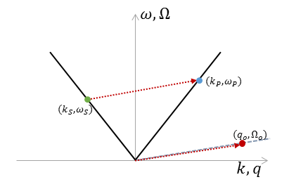
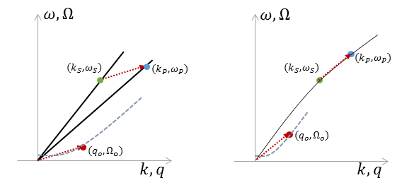
Figure 2: Phase-matching diagrams for backward SBS (top), forward intermodal (bottom left) and forward intramodal SBS (bottom right). Black lines represent optical dispersion relations, dashed blue lines represent acoustic dispersion relations.

Then we can write (IV) as

$$V = \int\mathrm{d}z\,\int\frac{\mathrm{d}k\mathrm{d}k^{\prime}\mathrm{d}q}{\left(2\pi\right)^{3/2}}\;a_{\text{\tiny P}k}^{\dagger}\mathrm{e}^{-i(k-k_{\text{\tiny P}})z}a_{\text{\tiny S}k^{\prime}}\mathrm{e}^{i(k^{\prime}-k_{\text{\tiny S}})z}b_{\alpha_{\text{\tiny o}}q}\mathrm{e}^{i(q-q_{\text{\tiny o}})z}\;\Gamma(\gamma_{\text{\tiny P}}k;\gamma_{\text{\tiny S}}k^{\prime};\alpha_{\text{\tiny o}}q)$$

$$+\int\mathrm{d}z\,\int\frac{\mathrm{d}k\mathrm{d}k^{\prime}\mathrm{d}q}{(2\pi)^{3/2}}\;b_{\alpha_{\text{\tiny o}}q}^{\dagger}\mathrm{e}^{-i(q-q_{\text{\tiny o}})z}a_{\text{\tiny S}k^{\prime}}^{\dagger}\mathrm{e}^{-i(k^{\prime}-k_{\text{\tiny S}})z}a_{\text{\tiny P}k}\mathrm{e}^{i(k-k_{\text{\tiny P}})z}\;\Gamma^{*}(\gamma_{\text{\tiny P}}k;\gamma_{\text{\tiny S}}k^{\prime};\alpha_{\text{\tiny o}}q).$$

Given the narrow bandwidths associated with SBS, we treat the coupling strengths $\Gamma(\gamma_{\text{\tiny P}}k;\gamma_{\text{\tiny S}}k^{\prime};\alpha_{\text{\tiny o}}q)$ as constant over the range of wavenumbers integration:

$$\Gamma(\gamma_{\text{\tiny P}}k;\gamma_{\text{\tiny S}}k^{\prime};\alpha_{\text{\tiny o}}q)\approx\Gamma(\gamma_{\text{\tiny P}}k_{\text{\tiny P}};\gamma_{\text{\tiny S}}k_{\text{\tiny S}};\alpha_{\text{\tiny o}}q_{\text{\tiny o}})\equiv\Gamma.$$ (70)

Pulling this term out, moving to the Heisenberg picture and using the definitions of the envelope functions in Eqs. (32) and (49), we reach

$$V=\Gamma\int\mathrm{d}z\,\psi_{\text{\tiny P}}^{\dagger}(z,t)\psi_{\text{\tiny S}}(z,t)\phi(z,t)+\Gamma^{*}\int\mathrm{d}z\,\phi^{\dagger}(z,t)\psi_{\text{\tiny S}}^{\dagger}(z,t)\psi_{\text{\tiny P}}(z,t),$$ (71)

where $\psi_{\text{\tiny S}}$, $\psi_{\text{\tiny S}}$, $\phi$ are the pump and Stokes photon fields and phonon fields respectively. Using (34) and (56), we find

$$\frac{\partial\psi_{\text{\tiny P}}(z,t)}{\partial t} =\frac{1}{i\hbar}\left[\psi_{\text{\tiny P}}(z,t),H^{\text{EM}}\right]+\frac{1}{i\hbar}\left[\psi_{\text{\tiny P}}(z,t),V\right]$$

$$=-i\omega_{\text{\tiny P}}\psi_{\text{\tiny P}}(z,t)-v_{\text{\tiny P}}\frac{\partial\psi_{\text{\tiny P}}(z,t)}{\partial z}+\frac{1}{2}iv_{\text{\tiny P}}^{\prime}\frac{\partial^{2}\psi_{\text{\tiny P}}(z,t)}{\partial z^{2}}+\frac{\Gamma}{i\hbar}\psi_{\text{\tiny S}}(z,t)\phi(z,t),$$ (72a)

and similarly

$$\frac{\partial\psi_{\text{\tiny S}}(z,t)}{\partial t} =-i\omega_{\text{\tiny S}}\psi_{\text{\tiny S}}(z,t)-v_{\text{\tiny S}}\frac{\partial\psi_{\text{\tiny S}}(z,t)}{\partial z}+\frac{1}{2}iv_{\text{\tiny S}}^{\prime}\frac{\partial^{2}\psi_{\text{\tiny S}}(z,t)}{\partial z^{2}}+\frac{\Gamma^{*}}{i\hbar}\phi^{\dagger}(z,t)\psi_{\text{\tiny P}}(z,t),$$ (72b)

$$\frac{\partial\phi(z,t)}{\partial t} =-i\Omega_{\text{\tiny o}}\phi(z,t)-v_{\text{\tiny o}}\frac{\partial\phi(z,t)}{\partial z}+\frac{1}{2}iv_{\text{\tiny o}}^{\prime}\frac{\partial^{2}\phi(z,t)}{\partial z^{2}}+\frac{\Gamma^{*}}{i\hbar}\psi_{\text{\tiny S}}^{\dagger}(z,t)\psi_{\text{\tiny P}}(z,t).$$ (72c)

To remove the fast time-dependence, we define

$$\Psi_{\text{\tiny P}}(z,t) =\psi_{\text{\tiny P}}(z,t)\sqrt{\hbar\omega_{\text{\tiny P}}|v_{\text{\tiny P}}|}\mathrm{e}^{i\omega_{\text{\tiny P}}t},$$ (73a)

$$\Psi_{\text{\tiny S}}(z,t) =\psi_{\text{\tiny S}}(z,t)\sqrt{\hbar\omega_{\text{\tiny S}}|v_{\text{\tiny S}}|}\mathrm{e}^{i\omega_{\text{\tiny S}}t},$$ (73b)

$$\Phi(z,t) =\phi(z,t)\sqrt{\hbar\Omega_{o}|v_{\text{\tiny o}}|}\mathrm{e}^{i\Omega_{\text{\tiny o}}t},$$ (73c)

so that

$$\Psi_{\text{\tiny P}}^{\dagger}(z,t)\Psi_{\text{\tiny P}}(z,t) = \hbar\omega_{\text{\tiny P}}\left|v_{\text{\tiny P}}\right|\,\psi_{\text{\tiny P}}^{\dagger}(z,t){\psi}_{\text{\tiny P}}(z,t),$$

$$\Psi_{\text{\tiny S}}^{\dagger}(z,t)\Psi_{\text{\tiny S}}(z,t) = \hbar\omega_{\text{\tiny S}}\left|v_{\text{\tiny S}}\right|\,\psi_{\text{\tiny S}}^{\dagger}(z,t){\psi}_{\text{\tiny S}}(z,t),$$

$$\Phi^{\dagger}(z,t)\Phi(z,t) = \hbar\Omega_{\text{\tiny o}}\left|v_{\text{\tiny o}}\right|\,\phi^{\dagger}(z,t){\phi}(z,t).$$

Thus $\Psi_{\text{\tiny P}}^{\dagger}(z,t)\Psi_{\text{\tiny P}}(z,t)$, $\Psi_{\text{\tiny S}}^{\dagger}(z,t)\Psi_{\text{\tiny S}}(z,t)$, and $\Phi^{\dagger}(z,t)\Phi(z,t)$ can be identified as the power flowing in the waveguide in each mode at position $z$; this is a positive quantity with the direction along $z$ given by the sign of the velocity.

Defining a reduced coupling constant

$$\bar{\Gamma}(\gamma k;\gamma{{}^{\prime}}k^{\prime};\alpha q)=\frac{1}{\sqrt{\left(\hbar\omega_{\gamma k}\right)\left(\hbar\omega_{\gamma{{}^{\prime}}k^{\prime}}\right)\left(\hbar{\Omega_{\alpha q}}\right)\left|v_{\gamma k}v_{\gamma{{}^{\prime}}k^{\prime}}v_{\alpha q}\right|}}\Gamma(\gamma k;\gamma{{}^{\prime}}k^{\prime};\alpha q),$$ (74)

and evaluating it at the center frequencies of our equations:

$$\bar{\Gamma}_{0}=\frac{1}{\sqrt{\left(\hbar\omega_{\text{\tiny P}}\right)\left(\hbar\omega_{\text{\tiny S}}\right)\left(\hbar\Omega_{\text{\tiny o}}\right)\left|v_{\text{\tiny P}}v_{\text{\tiny S}}v_{\text{\tiny o}}\right|}}\Gamma(\gamma_{\text{\tiny P}}k_{\text{\tiny P}};\gamma_{\text{\tiny S}}k_{\text{\tiny S}};\alpha_{\text{\tiny o}}q_{\text{\tiny o}}),$$ (75)

we obtain the Heisenberg evolution equations for the field operators

$$\frac{\partial\Psi_{\text{\tiny P}}(z,t)}{\partial t}+v_{\text{\tiny P}}\frac{\partial\Psi_{\text{\tiny P}}(z,t)}{\partial z}-\frac{1}{2}iv_{\text{\tiny P}}^{\prime}\frac{\partial^{2}\Psi_{\text{\tiny P}}(z,t)}{\partial z^{2}} = -i\omega_{\text{\tiny P}}\left|v_{\text{\tiny P}}\right|\bar{\Gamma}_{0}\;\Psi_{\text{\tiny S}}(z,t)\Phi(z,t),$$ (76a)

$$\frac{\partial\Psi_{\text{\tiny S}}(z,t)}{\partial t}+v_{\text{\tiny S}}\frac{\partial\Psi_{\text{\tiny S}}(z,t)}{\partial z}-\frac{1}{2}iv_{\text{\tiny S}}^{\prime}\frac{\partial^{2}\Psi_{\text{\tiny S}}(z,t)}{\partial z^{2}} = -i\omega_{\text{\tiny S}}\left|v_{\text{\tiny S}}\right|\bar{\Gamma}_{0}^{*}\;\Phi^{\dagger}(z,t)\Psi_{\text{\tiny P}}(z,t),$$ (76b)

$$\frac{\partial\Phi(z,t)}{\partial t}+v_{\text{\tiny o}}\frac{\partial\Phi(z,t)}{\partial z}-\frac{1}{2}iv_{\text{\tiny o}}^{\prime}\frac{\partial^{2}\Phi(z,t)}{\partial z^{2}} = -i\Omega_{\text{\tiny o}}\left|v_{\text{\tiny o}}\right|\bar{\Gamma}_{0}^{*}\;\Psi_{\text{\tiny S}}^{\dagger}(z,t)\Psi_{\text{\tiny P}}(z,t).$$ (76c)

We have thus established a fully quantum form of the opto-acoustic coupled evolution equations and shown that the correspondence of coupling constants for photoelasticity plus moving boundaries and the reverse processes of electrostriction plus radiation pressure emerge naturally from the starting point of (60). We next evaluate the coupling constants (or “matrix elements”) to connect them to familiar forms in the literature.

V.1 The coupling constants

We separate the coupling constants $\bar{\Gamma}(\gamma k;\gamma{{}^{\prime}}k^{\prime};\alpha q)$ in Eq. (74) into the contributions

$$\bar{\Gamma}(\gamma k;\gamma{{}^{\prime}}k^{\prime};\alpha q)=\bar{\Gamma}_{\text{bulk}}(\gamma k;\gamma{{}^{\prime}}k^{\prime};\alpha q)+\Gamma_{\text{surf}}(\gamma k;\gamma{{}^{\prime}}k^{\prime};\alpha q),$$ (77)

where

$$\bar{\Gamma}_{\text{bulk}}(\gamma k;\gamma{{}^{\prime}}k^{\prime};\alpha q) = \frac{1}{\epsilon_{0}}\frac{1}{2\sqrt{2}\left|v_{\gamma k}v_{\gamma{{}^{\prime}}k^{\prime}}v_{\alpha q}\right|}\int\mathrm{d}x\mathrm{d}y\,\left(d_{\gamma k}^{i}(x,y)\right)^{*}d_{\gamma{{}^{\prime}}k^{\prime}}^{j}(x,y)p^{ijlm}(x,y)s_{\alpha q}^{lm}(x,y),$$ (78)

and

$$\bar{\Gamma}_{\text{surf}}(\gamma k;\gamma{{}^{\prime}}k^{\prime};\alpha q) = -\frac{1}{\epsilon_{0}}\frac{1}{2\sqrt{2}\left|v_{\gamma k}v_{\gamma{{}^{\prime}}k^{\prime}}v_{\alpha q}\right|}\int\mathrm{d}x\mathrm{d}y\,\left(d_{\gamma k}^{i}(x,y)\right)^{*}d_{\gamma{{}^{\prime}}k^{\prime}}^{i}(x,y)\left(\frac{\partial\beta_{\text{ref}}(x,y)}{\partial r^{j}}\right)u_{\alpha q}^{j}(x,y).$$ (79)

The label “surface” for Eq. (79) is perhaps too restrictive since the derivative $\partial\beta_{\text{ref}}/\partial r^{j}$ is non-zero in graded index materials, however this contribution is typically weak, and in current experiments it is the surface contribution that is of most interest. We seek expressions in terms of the optical modes $\mathbf{d}_{\gamma k}$ and acoustic modes $\mathbf{u}_{\alpha q}$ that can be obtained from numerical solvers.

V.1.1 The bulk coupling constant

The bulk term in (78) describes photoelasticity (in (76a) and (76b)) and electrostriction (in (76c)). Its evaluation is straightforward. Even in the limit of a step discontinuity in material parameters across a waveguide interface, the $\mathbf{d}_{\gamma k}(x,y)$ will suffer at most a step discontinuity, as will $s_{\alpha q}^{lm}(x,y)$ and, by assumption, $p^{ijlm}(x,y)$. Hence (78) remains well-defined for step discontinuities.

Using the definition of $s_{\alpha q}^{lm}(x,y)$, one can show that for the standard interaction with modes $(\text{\tiny P},\text{\tiny S},\text{\tiny o})$, the bulk element reduces to the form

$$\bar{\Gamma}_{\text{bulk}}=\frac{1}{2^{3/2}\sqrt{|v_{\text{\tiny P}}v_{\text{\tiny S}}v_{\text{\tiny o}}|}}\frac{1}{\epsilon_{0}}\int\mathrm{d}x\mathrm{d}y\,d_{S}^{i}(x,y)(d_{\text{\tiny P}}^{j}(x,y))^{*}p^{ijlm}(x,y)\left[\left(\frac{\partial}{\partial r_{l}}u_{m}(x,y)\right)+iq\delta_{mz}(u_{l}(x,y))^{*}\right].$$ (80)

which is consistent with the results in Wolff et al. Wolff et al. (2015) for the photoelastic coupling, there termed $\Gamma^{\mathrm{ePE}}$.

V.1.2 The surface matrix element

The surface term in (79) describes driving of the optical fields by moving boundaries (in (76a) and (76b)) and radiation pressure (in (76c)). Its evaluation is more subtle, since in the limit of a step discontinuity in material parameters $\beta_{\text{ref}}(x,y)$ will change in a step-like fashion, but its derivative can be Dirac delta-function-like. Consequently, a smoothing operation is required to make sense of this term. Following Johnson et al. Johnson et al. (2002) one can show (see section S.IX of the supplementary material) that for a boundary contour $\mathbf{R}_{c}(s)$ parameterized by arc length $s$ that separates two materials with dielectric constants $\epsilon_{+}$ and $\epsilon_{-}$ the surface contribution reduces to

$$\bar{\Gamma}_{\text{surf}}(\gamma k;\gamma{{}^{\prime}}k^{\prime};\alpha q)=\frac{1}{2^{3/2}\sqrt{\left|v_{\gamma k}v_{\gamma{{}^{\prime}}k^{\prime}}v_{\alpha q}\right|}}\\ \times\left[\frac{1}{\epsilon_{0}}(\frac{1}{\epsilon_{-}}-\frac{1}{\epsilon_{+}})\int\left[d_{\gamma k}^{\perp}(\mathbf{R}_{c}(s))\right]^{\ast}d_{\gamma{{}^{\prime}}k^{\prime}}^{\perp}(\mathbf{R}_{c}(s))\left[\hat{\mathbf{n}}(s)\cdot\mathbf{u}_{\alpha q}(\mathbf{R}_{c}(s))\right]\,\mathrm{d}R_{c}(s)\right.\\ \left.+\epsilon_{0}\left(\epsilon_{+}-\epsilon_{-}\right)\int\left[\mathbf{e}_{\gamma k}^{\parallel}(\mathbf{R}_{c}(s))\right]^{*}\cdot\mathbf{e}_{\gamma{{}^{\prime}}k^{\prime}}^{\parallel}(\mathbf{R}_{c}(s))\,\left[\hat{\mathbf{n}}(s)\cdot\mathbf{u}_{\alpha q}(\mathbf{R}_{c}(s))\right]\,\mathrm{d}R_{c}(s)\right].$$ (81)

Here the unit normal $\hat{\mathbf{n}}(s)$ points in the direction from $\epsilon_{-}$ to $\epsilon_{+}$. The full expression for $\Gamma_{\text{surf}}(\gamma k;\gamma{{}^{\prime}}k^{\prime};\alpha q)$ then involves a sum over all such curves separating distinct dielectrics. Note there is no ambiguity in evaluating these terms, since $d_{\gamma k}^{\perp}(\mathbf{r})$ is continuous across a step discontinuity in $\beta_{\text{ref}}(x,y)$, as is $\mathbf{e}_{\gamma k}^{\parallel}(\mathbf{r}).$

For the SBS combination of modes $(\text{\tiny P},\text{\tiny S},\text{\tiny o})$, the surface term can also be written as

$$\bar{\Gamma}^{\text{MB}} =\left(\frac{1}{2\sqrt{2}\sqrt{|v_{\text{\tiny P}}v_{S}v_{\text{\tiny o}}|}}\int\mathrm{d}R_{c}(s)\,(\mathbf{u}^{*}\cdot\hat{\mathbf{n}})\left[\frac{1}{\epsilon_{0}}\left(\frac{1}{\epsilon_{-}}-\frac{1}{\epsilon_{+}}\right)(\mathbf{d}_{S}^{\perp})^{*}\mathbf{d}_{\text{\tiny P}}^{\perp}+\epsilon_{0}(\epsilon_{-}-\epsilon_{+})(\hat{\mathbf{n}}\times\mathbf{e}_{S})^{*}\cdot(\hat{\mathbf{n}}\times\mathbf{e}_{\text{\tiny P}})\right]\right)^{*},$$ (82)

which coincides with the expression of Wolff et al. Wolff et al. (2015).

A normalized form of these expressions convenient for working with numerical mode solvers is provided in section S.X of the supplementary material.

V.2 Recovery of classical coupled mode equations

Finally, the standard classical coupled mode equations Wolff et al. (2015) can be recovered from (76) by dropping the dispersion terms and taking mean values for the operators:

$$\frac{\partial{\left\langle\psi_{\text{\tiny P}}\right\rangle}}{\partial t}+v_{\text{\tiny P}}\frac{\partial{\left\langle\psi_{\text{\tiny P}}\right\rangle}}{\partial z} = -i\omega_{\text{\tiny P}}\left|v_{\text{\tiny P}}\right|\bar{\Gamma}_{0}\;{\left\langle\psi_{\text{\tiny S}}\right\rangle}{\left\langle\phi\right\rangle},$$ (83a)

$$\frac{\partial{\left\langle\psi_{\text{\tiny S}}\right\rangle}}{\partial t}+v_{\text{\tiny S}}\frac{\partial{\left\langle\psi_{\text{\tiny S}}\right\rangle}}{\partial z} = -i\omega_{\text{\tiny S}}\left|v_{\text{\tiny S}}\right|\bar{\Gamma}_{0}^{*}\;{\left\langle\phi\right\rangle}^{*}{\left\langle\psi_{\text{\tiny P}}\right\rangle},$$ (83b)

$$\frac{\partial{\left\langle\phi\right\rangle}}{\partial t}+v_{\text{\tiny o}}\frac{\partial{\left\langle\phi\right\rangle}}{\partial z}+v_{\text{\tiny o}}\alpha\langle\phi\rangle = -i\Omega_{\text{\tiny o}}\left|v_{\text{\tiny o}}\right|\bar{\Gamma}_{0}^{*}\;{\left\langle\psi_{\text{\tiny S}}\right\rangle}^{*}{\left\langle\psi_{\text{\tiny P}}\right\rangle}.$$ (83c)

We have introduced the acoustic loss $\alpha$ by hand following the expression of Wolff et al. Wolff et al. (2015):

$$\alpha=\frac{\Omega_{o}^{2}}{v_{\text{\tiny o}}}\int\mathrm{d}x\mathrm{d}y\,u_{i}^{*}\partial_{j}(\eta_{ijkl}\partial_{k}u_{l}),$$ (84)

where $\eta_{ijkl}$ is the viscosity tensor.

VI Discussion

Equations (76) represent a full quantum description of guided-wave optoacoustic interactions. Although it requires some preliminary derivations to identify the effective fields that are involved, our approach provides a direct derivation of both the photoelastic/electrostrictive and moving-boundaries/radiation pressure components of the SBS interaction. The latter has clear contributions from both surface effects at material boundaries and bulk effects due to smooth variation in dielectric properties. By avoiding any discussion of forces and stress tensors, the ambiguities and challenges of prior treatments do not arise.

The equations of motion have a number of potential applications. In the classical limit they provide a rigorous confirmation of the earlier treatment Wolff et al. (2015). In the quantum regime, we have a theory of opto-acoustic interactions that faithfully represents the photon and number statistics including any non-classical behavior. To date, quantum acoustic effects in guided wave systems have not been observed due to the overwhelming thermal contribution to the phonon field, though this may change in the near future. However, we can certainly envisage mixed systems in which a classical coherent state phonon field interacts with non-classical photon states in order to transfer quantum information between different channels, and our treatment is ideal for studies at this quantum-classical boundary.

An obvious and significant extension to our work would be a complete treatment of the acoustic dissipation, which we plan to present in the future. To incorporate dissipation into a Hamiltonian picture, a natural approach would be to introduce a thermal bath of phonon oscillators rather than just the Brillouin excited mode. These modes would couple with the coherent modes of interest and with each other through a three-phonon collision term associated with anharmonicity in the phonon Hamiltonian. Tracing over the additional oscillators would lead to an effective dissipation on the preferred phonon mode. According to need or preference, one could derive a dissipative master equation for the reduced phonon density operator, or perhaps more usefully, a set of Heisenberg equations with Langevin noise terms associated with the loss. This kind of treatment would be particularly important in understanding the impact of phonon loss on the photon quantum noise.

As mentioned earlier, another avenue is the description of enhancement and inhibition of SBS through density of states engineering Merklein et al. (2015). In the spontaneous regime, this is well handled by a Fermi Golden Rule calculation of phonon generation rates Sipe (2015), as we will demonstrate in a subsequent work.

S.I Heisenberg equations for acoustic field

In this section, we derive the equations of motion (8) in section II of the main paper.

Using Eqs. (50) and (7) we can derive the relations

$$\frac{\partial u^{n}(\mathbf{r},t)}{\partial t} = \frac{1}{i\hbar}\left[u^{n}(\mathbf{r}),H\right]$$

$$= \frac{1}{i\hbar}\int\frac{\left[u^{n}(\mathbf{r}),\pi^{i}(\mathbf{r^{\prime}})\right]\pi^{i}(\mathbf{r^{\prime}})}{2\rho(\mathbf{r^{\prime}})}\,\mathrm{d}\mathbf{r^{\prime}}+\frac{1}{i\hbar}\int\frac{\pi^{i}(\mathbf{r^{\prime}})\left[u^{n}(\mathbf{r}),\pi^{i}(\mathbf{r^{\prime}})\right]}{2\rho(\mathbf{r^{\prime}})}\,\mathrm{d}\mathbf{r^{\prime}}$$

$$= \delta^{ni}\int\frac{\delta(\mathbf{r}-\mathbf{r^{\prime}})\pi^{i}(\mathbf{r^{\prime}})}{2\rho(\mathbf{r^{\prime}})}\,\mathrm{d}\mathbf{r}^{\prime}+\delta^{ni}\int\frac{\pi^{i}(\mathbf{r^{\prime}})\delta(\mathbf{r}-\mathbf{r^{\prime}})}{2\rho(\mathbf{r^{\prime}})}\,\mathrm{d}\mathbf{r^{\prime}}$$

$$= \frac{\pi^{n}(\mathbf{r})}{\rho(\mathbf{r})},$$

and

$$\frac{\partial\pi^{n}(\mathbf{r},t)}{\partial t} = \frac{1}{i\hbar}\left[\pi^{n}(\mathbf{r}),H\right]$$

$$= \frac{1}{i\hbar}\frac{1}{2}\int\frac{\partial\left[\pi^{n}(\mathbf{r}),u^{i}(\mathbf{r^{\prime}})\right]}{\partial{r^{\prime}}^{j}}c^{ijkl}(\mathbf{r^{\prime}})\frac{\partial u^{k}(\mathbf{r^{\prime}})}{\partial{r^{\prime}}^{l}}\,\mathrm{d}\mathbf{r^{\prime}}+\frac{1}{i\hbar}\frac{1}{2}\int\frac{\partial u^{i}(\mathbf{r^{\prime}})}{\partial{r^{\prime}}^{j}}c^{ijkl}(\mathbf{r^{\prime}})\frac{\partial\left[\pi^{n}(\mathbf{r}),u^{k}(\mathbf{r^{\prime}})\right]}{\partial r^{\prime l}}\,\mathrm{d}\mathbf{r^{\prime}}$$

$$= -\frac{1}{2}\delta^{ni}\int\frac{\partial\delta(\mathbf{r-r}^{\prime})}{\partial{r^{\prime}}^{j}}c^{ijkl}(\mathbf{r^{\prime}})\frac{\partial u^{k}(\mathbf{r^{\prime}})}{\partial{r^{\prime}}^{l}}\,\mathrm{d}\mathbf{r}^{\prime}-\frac{1}{2}\delta^{nk}\int\frac{\partial u^{i}(\mathbf{r}^{\prime})}{\partial{r^{\prime}}^{j}}c^{ijkl}(\mathbf{r^{\prime}})\frac{\partial\delta(\mathbf{r}-\mathbf{r^{\prime}})}{\partial{r^{\prime}}^{l}}\,\mathrm{d}\mathbf{r}^{\prime}$$

$$= \frac{1}{2}\int\delta(\mathbf{r}-\mathbf{r^{\prime}})\left(\frac{\partial}{\partial{r^{\prime}}^{j}}\left(c^{njkl}(\mathbf{r^{\prime}})\frac{\partial u^{k}(\mathbf{r^{\prime}})}{\partial{r^{\prime}}^{l}}\right)\right)\,\mathrm{d}\mathbf{r^{\prime}}+\frac{1}{2}\int\left(\frac{\partial}{\partial{r^{\prime}}^{l}}\left(c^{ijnl}(\mathbf{r^{\prime}})\frac{\partial u^{i}(\mathbf{r}^{\prime})}{\partial{r^{\prime}}^{j}}\right)\right)\delta(\mathbf{r-r}^{\prime})\,\mathrm{d}\mathbf{r^{\prime}},$$

$$= \frac{1}{2}\frac{\partial}{\partial r^{j}}\left(c^{njkl}(\mathbf{r})\frac{\partial u^{k}(\mathbf{r})}{\partial r^{l}}\right)+\frac{1}{2}\frac{\partial}{\partial r^{l}}\left(c^{ijnl}(\mathbf{r})\frac{\partial u^{i}(\mathbf{r)}}{\partial r^{j}}\right)$$

$$= \frac{\partial}{\partial r^{j}}\left(c^{njkl}(\mathbf{r})\frac{\partial u^{k}(\mathbf{r})}{\partial r^{l}}\right)$$

$$= \frac{\partial}{\partial r^{j}}\big{(}c^{njkl}(\mathbf{r})S^{kl}(\mathbf{r})\big{)},$$

where in the second last line we have used (5).

S.II Operator $\mathcal{M}^{nk}(\mathbf{r})$ is Hermitian

Here we show that the operator $\mathcal{M}^{nk}(\mathbf{r})$ of (15) is Hermitian. Consider an integral over an appropriate volume and assume that fields are either periodic over the volume or vanish at the surface of the volume. Then for vector functions $\mathbf{C(\mathbf{r})}$ and $\mathbf{D(\mathbf{r})}$, integrating by parts twice gives

$$\int\left(D^{n}(\mathbf{r})\right)^{*}\left(\mathcal{M}^{nk}(\mathbf{r})C^{k}(\mathbf{r})\right)\mathrm{d}\mathbf{r} = -\int\frac{\left(D^{n}(\mathbf{r})\right)^{*}}{\rho^{1/2}(\mathbf{r})}\frac{\partial}{\partial r^{j}}\left(c^{njkl}(\mathbf{r})\frac{\partial}{\partial r^{l}}\left(\frac{C^{k}(\mathbf{r})}{\rho^{1/2}(\mathbf{r})}\right)\right)\mathrm{d}\mathbf{r}$$

$$= \int\left(\frac{\partial}{\partial r^{j}}\left(\frac{\left(D^{n}(\mathbf{r})\right)^{*}}{\rho^{1/2}(\mathbf{r})}\right)\right)\left(c^{njkl}(\mathbf{r})\frac{\partial}{\partial r^{l}}\left(\frac{C^{k}(\mathbf{r})}{\rho^{1/2}(\mathbf{r})}\right)\right)\mathrm{d}\mathbf{r}$$

$$= -\int\frac{C^{k}(\mathbf{r})}{\rho^{1/2}(\mathbf{r})}\frac{\partial}{\partial r^{l}}\left(c^{njkl}(\mathbf{r})\left(\frac{\partial}{\partial r^{j}}\left(\frac{\left(D^{n}(\mathbf{r})\right)^{*}}{\rho^{1/2}(\mathbf{r})}\right)\right)\right)\mathrm{d}\mathbf{r}$$

Now using (5) we put $c^{njkl}(\mathbf{r})=c^{klnj}(\mathbf{r})$ and switching the dummy indices $j\leftrightarrow l$, we can write this as

$$\int\left(D^{n}(\mathbf{r})\right)^{*}\left(\mathcal{M}^{nk}(\mathbf{r})C^{k}(\mathbf{r})\right)\mathrm{d}\mathbf{r} = -\int\frac{C^{k}(\mathbf{r})}{\rho^{1/2}(\mathbf{r})}\frac{\partial}{\partial r^{j}}\left(c^{kjnl}(\mathbf{r})\left(\frac{\partial}{\partial r^{l}}\left(\frac{\left(D^{n}(\mathbf{r})\right)^{*}}{\rho^{1/2}(\mathbf{r})}\right)\right)\right)\mathrm{d}\mathbf{r}$$

$$= \left(-\int\frac{\left(C^{k}(\mathbf{r})\right)^{*}}{\rho^{1/2}(\mathbf{r})}\frac{\partial}{\partial r^{j}}\left(c^{kjnl}(\mathbf{r})\left(\frac{\partial}{\partial r^{l}}\left(\frac{\left(D^{n}(\mathbf{r})\right)}{\rho^{1/2}(\mathbf{r})}\right)\right)\right)\mathrm{d}\mathbf{r}\right)^{*}$$

$$= \left(\int\left(C^{k}(\mathbf{r}\right))^{*}\left(\mathcal{M}^{kn}(\mathbf{r})D^{n}(\mathbf{r})\right)\mathrm{d}\mathbf{r}\right)^{*},$$

and so the differential operator $\mathcal{M}^{nk}(\mathbf{r})$ is Hermitian.

S.III Properties of mode functions and partner functions

Here we establish some useful properties of the mode functions $\mathbf{F}_{\Lambda}(\mathbf{r})$ introduced in (17) to (20), that are required to reduce the acoustic Hamiltonian to canonical harmonic oscillator form in S.IV.

Note that since $\mathcal{M}^{nk}(\mathbf{r})$ is real, if $\mathbf{F}_{\Lambda}(\mathbf{r})$ is an eigenfunction then $\mathbf{F}_{\Lambda}^{\ast}(\mathbf{r)}$ is also an eigenfunction with the same eigenvalue $\omega_{\Lambda}$. This may happen simply because $\mathbf{F}_{\Lambda}(\mathbf{r})$ is purely real. In fact, as we show in S.XI, it is always possible to choose the set of eigenfunctions $\left\{\mathbf{F}_{\Lambda}(\mathbf{r})\right\}$ such that each of them is purely real. But it is often more convenient to work with complex eigenfunctions (traveling waves rather than standing waves, for example). Section S.XI establishes that if we include complex eigenfunctions in the set $\left\{\mathbf{F}_{\Lambda}(\mathbf{r})\right\}$, the set can be chosen so that each eigenfunction $\mathbf{F}_{\Lambda}(\mathbf{r})$ is either real or, if not, there is another eigenfunction $\mathbf{F}_{\bar{\Lambda}}(\mathbf{r})$ in the set such that $\mathbf{F}_{\bar{\Lambda}}(\mathbf{r})=\mathbf{F}_{\Lambda}^{\ast}(\mathbf{r})$.

Typically the naturally chosen set of eigenfunctions will make this so; for example, if $\mathbf{F}_{\Lambda}(\mathbf{r})$ is a traveling wave to the right, then $\mathbf{F}_{\bar{\Lambda}}(\mathbf{r})$ is a traveling wave to the left. We refer to $\mathbf{F}_{\bar{\Lambda}}(\mathbf{r})$ as the “partner” of $\mathbf{F}_{\Lambda}(\mathbf{r})$. That is, each complex eigenfunction in the set has a partner that is also in the set. If there are purely real eigenfunctions in the set $\left\{\mathbf{F}_{\Lambda}(\mathbf{r})\right\}$, we take them to be their own partners.  Then the set of eigenfunctions $\left\{\mathbf{F}_{\Lambda}(\mathbf{r})\right\}$ is equivalent to the set of $\left\{\mathbf{F}_{\bar{\Lambda}}(\mathbf{r})\right\}$ of partner eigenfunctions, and $\mathbf{F}_{\bar{\Lambda}}(\mathbf{r})=\mathbf{F}_{\Lambda}^{\ast}(\mathbf{r})$ for each $\Lambda$. Since the set of partners is equivalent to the original set, then from Eq. (20) of the main paper we can also write

$$\int\mathbf{F}_{\bar{\Lambda}}^{\ast}(\mathbf{r})\cdot\mathbf{F}_{\bar{\Lambda}^{\prime}}(\mathbf{r})\,\mathrm{d}\mathbf{r}=\delta_{\bar{\Lambda}\bar{\Lambda}^{\prime}},$$ (S.1)

and

$$\sum_{\bar{\Lambda}}F_{\bar{\Lambda}}^{n}(\mathbf{r})\left(F_{\bar{\Lambda}}^{m}(\mathbf{r^{\prime}})\right)^{\ast}=\delta^{nm}\delta(\mathbf{r-r}^{\prime}).$$ (S.2)

Similarly, from Eq. (18) of the main paper we see that we have

$$\mathbf{\tilde{U}}_{\bar{\Lambda}}(\mathbf{r}) = \mathbf{\tilde{U}}_{\Lambda}^{\ast}(\mathbf{r}),$$ (S.3a)

$$\mathbf{\tilde{\Pi}}_{\bar{\Lambda}}(\mathbf{r}) = -\mathbf{\tilde{\Pi}}_{\Lambda}^{\ast}(\mathbf{r}).$$ (S.3b)

S.IV Acoustic mode expansion

Here we show that through use of the partner functions introduced in S.III, the acoustic field operators and Hamiltonian can be expanded in terms of the mode functions as expressed in Eqs. (22) and (23). Recall that the $\left\{\mathbf{F}_{\Lambda}(\mathbf{r})\right\}$ are the eigenfunctions of (15) and that the $\left\{\mathbf{\tilde{U}}_{\Lambda}(\mathbf{r})\right\}$ and $\left\{\mathbf{\tilde{\Pi}}_{\Lambda}(\mathbf{r})\right\}$ are defined as in Eq. (18). Both sets of functions are proportional to the $\left\{\mathbf{F}_{\Lambda}(\mathbf{r})\right\}$, so we can take each to constitute a complete set of states. We can then expand

$$\tilde{\mathbf{u}}(\mathbf{r}) = \sum_{\Lambda}\sqrt{\frac{\hbar}{2\Omega_{\Lambda}}}\mathcal{C}_{\Lambda}^{(1)}\mathbf{\tilde{U}}_{\Lambda}(\mathbf{r}),$$ (S.4)

$$\tilde{{\boldsymbol{\pi}}}(\mathbf{r}) = \sum_{\Lambda}\sqrt{\frac{\hbar}{2\Omega_{\Lambda}}}\mathcal{C}_{\Lambda}^{(2)}\mathbf{\tilde{\Pi}}_{\Lambda}(\mathbf{r}),$$

where $\mathcal{C}_{\Lambda}^{(1)}$ and $\mathcal{C}_{\Lambda}^{(2)}$ are operators and the factors $\sqrt{\hbar/2\Omega_{\Lambda}}$ are added for later convenience.

In the Heisenberg picture, $\mathcal{C}_{\Lambda}^{(1)}$ and $\mathcal{C}_{\Lambda}^{(2)}$ are time-dependent, and therefore so are $\tilde{\mathbf{u}}(\mathbf{r})$ and $\tilde{{\boldsymbol{\pi}}}(\mathbf{r})$. However, since $\tilde{\mathbf{u}}(\mathbf{r})$ and $\tilde{{\boldsymbol{\pi}}}(\mathbf{r})$ are Hermitian the $\left\{\mathcal{C}_{\Lambda}^{(1)}\right\}$ are not all independent, nor are the $\left\{\mathcal{C}_{\Lambda}^{(2)}\right\}$. Using Eqs. (S.3) we have

$$\tilde{\mathbf{u}}^{\dagger}(\mathbf{r}) = \sum_{\Lambda}\sqrt{\frac{\hbar}{2\Omega_{\Lambda}}}\left(\mathcal{C}_{\Lambda}^{(1)}\right)^{\dagger}\mathbf{\tilde{U}}_{\Lambda}^{\ast}(\mathbf{r})=\sum_{\Lambda}\sqrt{\frac{\hbar}{2\Omega_{\Lambda}}}\left(\mathcal{C}_{\Lambda}^{(1)}\right)^{\dagger}\mathbf{\tilde{U}}_{\bar{\Lambda}}(\mathbf{r})$$

$$\tilde{{\boldsymbol{\pi}}}^{\dagger}(\mathbf{r}) = \sum_{\Lambda}\sqrt{\frac{\hbar}{2\Omega_{\Lambda}}}\left(\mathcal{C}_{\Lambda}^{(2)}\right)^{\dagger}\mathbf{\tilde{\Pi}}_{\Lambda}^{\ast}(\mathbf{r})=-\sum_{\Lambda}\sqrt{\frac{\hbar}{2\Omega_{\Lambda}}}\left(\mathcal{C}_{\Lambda}^{(2)}\right)^{\dagger}\mathbf{\tilde{\Pi}}_{\bar{\Lambda}}(\mathbf{r}),$$

so that (S.4) may also be written as a sum over partner modes,

$$\tilde{\mathbf{u}} = \sum_{\Lambda}\sqrt{\frac{\hbar}{2\Omega_{\Lambda}}}\mathcal{C}_{\bar{\Lambda}}^{(1)}\mathbf{\tilde{U}}_{\bar{\Lambda}}(\mathbf{r}),$$

$$\tilde{{\boldsymbol{\pi}}} = \sum_{\Lambda}\sqrt{\frac{\hbar}{2\Omega_{\Lambda}}}\mathcal{C}_{\bar{\Lambda}}^{(2)}\mathbf{\tilde{\Pi}}_{\bar{\Lambda}}(\mathbf{r}),$$

where we have used $\Omega_{\bar{\Lambda}}=\Omega_{\Lambda}$. Then from the Hermiticity of the canonical fields we see that we require

$$\left(\mathcal{C}_{\Lambda}^{(1)}\right)^{\dagger} = \mathcal{C}_{\bar{\Lambda}}^{(1)},$$

$$-\left(\mathcal{C}_{\Lambda}^{(2)}\right)^{\dagger} = \mathcal{C}_{\bar{\Lambda}}^{(2)},$$

which may be satisfied by setting

$$\mathcal{C}_{\Lambda}^{(1)} = b_{\Lambda}+b_{\bar{\Lambda}}^{\dagger},$$ (S.5)

$$\mathcal{C}_{\Lambda}^{(2)} = b_{\Lambda}-b_{\bar{\Lambda}}^{\dagger}.$$

For real eigenfunctions $\mathbf{F}_{\Lambda}(\mathbf{r})$ we have $\bar{\Lambda}=\Lambda$ and this just says that $\mathcal{C}_{\Lambda}^{(1)}$ is (proportional to) a coordinate operator, and $\mathcal{C}_{\Lambda}^{(2)}$ is (proportional to) a momentum operator (as we will see). For partners, $b_{\Lambda}$ and $b_{\bar{\Lambda}}$ are independent operators (or independent amplitudes in the classical case). Using (S.5) in (S.4) we have

$$\tilde{\mathbf{u}}(\mathbf{r}) = \sum_{\Lambda}\sqrt{\frac{\hbar}{2\Omega_{\Lambda}}}\left(b_{\Lambda}+b_{\bar{\Lambda}}^{\dagger}\right)\mathbf{F}_{\Lambda}(\mathbf{r})$$

$$= \sum_{\Lambda}\sqrt{\frac{\hbar}{2\Omega_{\Lambda}}}b_{\Lambda}\mathbf{F}_{\Lambda}(\mathbf{r})+\sum_{\Lambda}\sqrt{\frac{\hbar}{2\Omega_{\Lambda}}}b_{\bar{\Lambda}}^{\dagger}\mathbf{F}_{\bar{\Lambda}}^{\ast}(\mathbf{r})$$

$$= \sum_{\Lambda}\sqrt{\frac{\hbar}{2\Omega_{\Lambda}}}b_{\Lambda}\mathbf{F}_{\Lambda}(\mathbf{r})+\sum_{\Lambda}\sqrt{\frac{\hbar}{2\Omega_{\Lambda}}}b_{\Lambda}^{\dagger}\mathbf{F}_{\Lambda}^{\ast}(\mathbf{r})$$

$$= \sum_{\Lambda}\sqrt{\frac{\hbar}{2\Omega_{\Lambda}}}b_{\Lambda}\mathbf{F}_{\Lambda}(\mathbf{r})+\text{h.c.},$$

where in the third line we use the fact that the sum is over the whole set of partner functions. Similarly

$$\tilde{{\boldsymbol{\pi}}}(\mathbf{r}) = \sum_{\Lambda}\left(-i\sqrt{\frac{\hbar\Omega_{\Lambda}}{2}}\right)\left(b_{\Lambda}-b_{\bar{\Lambda}}^{\dagger}\right)\mathbf{F}_{\Lambda}(\mathbf{r})$$

$$= -i\sum_{\Lambda}\sqrt{\frac{\hbar\Omega_{\Lambda}}{2}}b_{\Lambda}\mathbf{F}_{\Lambda}(\mathbf{r})+i\sum_{\Lambda}\sqrt{\frac{\hbar\Omega_{\Lambda}}{2}}b_{\bar{\Lambda}}^{\dagger}\mathbf{F}_{\bar{\Lambda}}^{\ast}(\mathbf{r})$$

$$= -i\sum_{\Lambda}\sqrt{\frac{\hbar\Omega_{\Lambda}}{2}}b_{\Lambda}\mathbf{F}_{\Lambda}(\mathbf{r})+i\sum_{\Lambda}\sqrt{\frac{\hbar\Omega_{\Lambda}}{2}}b_{\Lambda}^{\dagger}\mathbf{F}_{\Lambda}^{\ast}(\mathbf{r})$$

$$= -i\sum_{\Lambda}\sqrt{\frac{\hbar\Omega_{\Lambda}}{2}}b_{\Lambda}\mathbf{F}_{\Lambda}(\mathbf{r})+\text{h.c.}$$ (S.8)

in accordance with Eq. (22).

Postulating the commutation relations

$$\left[b_{\Lambda},b_{\Lambda^{\prime}}\right] = 0,$$ (S.9)

$$\left[b_{\Lambda},b_{\Lambda^{\prime}}^{\dagger}\right] = \delta_{\Lambda\Lambda^{\prime}},$$

we find

$$\left[\tilde{u}^{n}(\mathbf{r}),\tilde{\pi}^{m}(\mathbf{r^{\prime}})\right] = i\sum_{\Lambda,\Lambda^{\prime}}\sqrt{\frac{\hbar}{2\Omega_{\Lambda}}}\sqrt{\frac{\hbar\Omega_{\Lambda^{\prime}}}{2}}\left[b_{\Lambda},b_{\Lambda^{\prime}}^{\dagger}\right]F_{\Lambda}^{n}(\mathbf{r})\left(F_{\Lambda^{\prime}}^{m}(\mathbf{r^{\prime}})\right)^{\ast}$$ (S.10)

$$-i\sum_{\Lambda,\Lambda^{\prime}}\sqrt{\frac{\hbar}{2\Omega_{\Lambda}}}\sqrt{\frac{\hbar\Omega_{\Lambda^{\prime}}}{2}}\left[b_{\Lambda}^{\dagger},b_{\Lambda^{\prime}}\right]\left(F_{\Lambda}^{n}(\mathbf{r})\right)^{\ast}F_{\Lambda^{\prime}}^{m}(\mathbf{r^{\prime}})$$

$$= \frac{i\hbar}{2}\sum_{\Lambda}F_{\Lambda}^{n}(\mathbf{r})\left(F_{\Lambda}^{m}(\mathbf{r^{\prime}})\right)^{\ast}+\frac{i\hbar}{2}\sum_{\Lambda}\left(F_{\Lambda}^{n}(\mathbf{r})\right)^{\ast}F_{\Lambda}^{m}(\mathbf{r^{\prime}})$$

$$= \frac{i\hbar}{2}\sum_{\Lambda}F_{\Lambda}^{n}(\mathbf{r})\left(F_{\Lambda}^{m}(\mathbf{r^{\prime}})\right)^{\ast}+\frac{i\hbar}{2}\sum_{\Lambda}F_{\bar{\Lambda}}^{n}(\mathbf{r})\left(F_{\bar{\Lambda}}^{m}(\mathbf{r^{\prime}})\right)^{\ast}$$

$$= i\hbar\delta^{nm}\delta(\mathbf{r}-\mathbf{r^{\prime}}),$$

where we have used (20) and (S.2). Since $[\tilde{\mathbf{u}}^{m}(\mathbf{r}),\tilde{{\boldsymbol{\pi}}}^{m}(\mathbf{r})]=[{\mathbf{u}}^{m}(\mathbf{r}),{{\boldsymbol{\pi}}}^{m}(\mathbf{r})]$ we recover the starting commutation relations (2). It is possible but more complicated to show that demanding the result (S.10) one can find that the $b_{\Lambda}$ and $b_{\Lambda}^{\dagger}$ must satisfy (S.9).

Now we look at the Hamiltonian in terms of the $b_{\Lambda}$ and $b_{\Lambda}^{\dagger}$. From (16) we have

$$H^{\text{A}}=\frac{1}{2}\int\tilde{\pi}^{i}(\mathbf{r})\tilde{\pi}^{i}(\mathbf{r})\,\mathrm{d}\mathbf{r}+\frac{1}{2}\int\tilde{u}^{i}(\mathbf{r})\mathcal{M}^{ik}(\mathbf{r})\tilde{u}^{k}\,\mathrm{d}\mathbf{r}.$$

From the above we have

$$\tilde{u}^{i}\mathbf{(r}) = \sum_{\Lambda}\sqrt{\frac{\hbar}{2\Omega_{\Lambda}}}b_{\Lambda}F_{\Lambda}^{i}(\mathbf{r})+\sum_{\Lambda}\sqrt{\frac{\hbar}{2\Omega_{\Lambda}}}b_{\Lambda}^{\dagger}\left(F_{\Lambda}^{i}(\mathbf{r})\right)^{\ast},$$

$$\tilde{\pi}^{i}\mathbf{(r}) = -i\sum_{\Lambda}\sqrt{\frac{\hbar\Omega_{\Lambda}}{2}}b_{\Lambda}F_{\Lambda}^{i}(\mathbf{r})+i\sum_{\Lambda}\sqrt{\frac{\hbar\Omega_{\Lambda}}{2}}b_{\Lambda}^{\dagger}\left(F_{\Lambda}^{i}(\mathbf{r})\right)^{\ast},$$

so

$$\int\tilde{\pi}^{i}\mathbf{(r})\tilde{\pi}^{i}\mathbf{(r})\,\mathrm{d}\mathbf{r} = -\sum_{\Lambda,\Lambda^{\prime}}\frac{\hbar}{2}\sqrt{\Omega_{\Lambda}\Omega_{\Lambda^{\prime}}}b_{\Lambda}b_{\Lambda^{\prime}}\int F_{\Lambda}^{i}(\mathbf{r})F_{\Lambda^{\prime}}^{i}(\mathbf{r})\,\mathrm{d}\mathbf{r}$$

$$-\sum_{\Lambda,\Lambda^{\prime}}\frac{\hbar}{2}\sqrt{\Omega_{\Lambda}\Omega_{\Lambda^{\prime}}}b_{\Lambda}^{\dagger}\dagger b_{\Lambda^{\prime}}^{\dagger}\left(\int F_{\Lambda}^{i}(\mathbf{r})F_{\Lambda^{\prime}}^{i}(\mathbf{r})\,\mathrm{d}\mathbf{r}\right)^{\ast}$$

$$+\sum_{\Lambda,\Lambda^{\prime}}\frac{\hbar}{2}\sqrt{\Omega_{\Lambda}\Omega_{\Lambda^{\prime}}}b_{\Lambda}b_{\Lambda^{\prime}}^{\dagger}\int F_{\Lambda}^{i}(\mathbf{r})\left(F_{\Lambda^{\prime}}^{i}(\mathbf{r})\right)^{\ast}\,\mathrm{d}\mathbf{r}$$

$$+\sum_{\Lambda,\Lambda^{\prime}}\frac{\hbar}{2}\sqrt{\Omega_{\Lambda}\Omega_{\Lambda^{\prime}}}b_{\Lambda}^{\dagger}b_{\Lambda^{\prime}}\left(\int F_{\Lambda}^{i}(\mathbf{r})\left(F_{\Lambda^{\prime}}^{i}(\mathbf{r})\right)^{\ast}\,\mathrm{d}\mathbf{r}\right)^{\ast}.$$

In the last two terms, orthogonality gives $\Lambda^{\prime}=\Lambda$. In the first two, we replace the sum over $\Lambda$ by a sum over $\bar{\Lambda}$ and use the fact that $\mathbf{F}_{\Lambda}(\mathbf{r})=\mathbf{F}_{\bar{\Lambda}}^{\ast}(\mathbf{r})$; then orthogonality demands that $\Lambda^{\prime}=\bar{\Lambda}$. Recalling that $\Omega_{\bar{\Lambda}}=\Omega_{\Lambda}$ we then have

$$\int\tilde{\pi}^{i}\mathbf{(r})\tilde{\pi}^{i}\mathbf{(r})\,\mathrm{d}\mathbf{r} = -\frac{1}{2}\sum_{\Lambda}\hbar\Omega_{\Lambda}b_{\Lambda}b_{\bar{\Lambda}}-\frac{1}{2}\sum_{\Lambda}\hbar\Omega_{\Lambda}b_{\Lambda}^{\dagger}b_{\bar{\Lambda}}^{\dagger}$$

$$+\frac{1}{2}\sum_{\Lambda}\hbar\Omega_{\Lambda}b_{\Lambda}b_{\Lambda}^{\dagger}+\frac{1}{2}\sum_{\Lambda}\hbar\Omega_{\Lambda}b_{\Lambda}^{\dagger}b_{\Lambda}.$$

Then since

$$\mathcal{M}^{ik}(\mathbf{r})\tilde{u}^{k}(\mathbf{r}) = \sum_{\Lambda}\sqrt{\frac{\hbar}{2\Omega_{\Lambda}}}\Omega_{\Lambda}^{2}b_{\Lambda}F_{\Lambda}^{i}(\mathbf{r})+\sum_{\Lambda}\sqrt{\frac{\hbar}{2\Omega_{\Lambda}}}\Omega_{\Lambda}^{2}b_{\Lambda}^{\dagger}\left(F_{\Lambda}^{i}(\mathbf{r})\right)^{\ast},$$

we have

$$\int\tilde{u}^{i}(\mathbf{r})\mathcal{M}^{ik}(\mathbf{r})\tilde{u}^{k}(\mathbf{r})\,\mathrm{d}\mathbf{r} = \sum_{\Lambda,\Lambda^{\prime}}\frac{\hbar}{2\sqrt{\Omega_{\Lambda}\Omega_{\Lambda^{\prime}}}}\Omega_{\Lambda^{\prime}}^{2}b_{\Lambda}b_{\Lambda^{\prime}}\int F_{\Lambda}^{i}(\mathbf{r})F_{\Lambda^{\prime}}^{i}(\mathbf{r})\,\mathrm{d}\mathbf{r}$$

$$+\sum_{\Lambda,\Lambda^{\prime}}\frac{\hbar}{2\sqrt{\Omega_{\Lambda}\Omega_{\Lambda^{\prime}}}}\Omega_{\Lambda^{\prime}}^{2}b_{\Lambda}^{\dagger}b_{\Lambda^{\prime}}^{\dagger}\left(\int F_{\Lambda}^{i}(\mathbf{r})F_{\Lambda^{\prime}}^{i}(\mathbf{r})\,\mathrm{d}\mathbf{r}\right)^{\ast}$$

$$+\sum_{\Lambda,\Lambda^{\prime}}\frac{\hbar}{2\sqrt{\Omega_{\Lambda}\Omega_{\Lambda^{\prime}}}}\Omega_{\Lambda^{\prime}}^{2}b_{\Lambda}b_{\Lambda^{\prime}}^{\dagger}\int F_{\Lambda}^{i}(\mathbf{r})\left(F_{\Lambda^{\prime}}^{i}(\mathbf{r})\right)^{\ast}\,\mathrm{d}\mathbf{r}$$

$$+\sum_{\Lambda,\Lambda^{\prime}}\frac{\hbar}{2\sqrt{\Omega_{\Lambda}\Omega_{\Lambda^{\prime}}}}\Omega_{\Lambda^{\prime}}^{2}b_{\Lambda}^{\dagger}b_{\Lambda^{\prime}}\left(\int F_{\Lambda}^{i}(\mathbf{r})\left(F_{\Lambda^{\prime}}^{i}(\mathbf{r})\right)^{\ast}\,\mathrm{d}\mathbf{r}\right)^{\ast}.$$

Using the same strategy as above this gives

$$\int\tilde{u}^{i}(\mathbf{r})\mathcal{M}^{ik}(\mathbf{r})\tilde{u}^{k}(\mathbf{r})\,\mathrm{d}\mathbf{r} = \frac{1}{2}\sum_{\Lambda}\hbar\Omega_{\Lambda}b_{\Lambda}b_{\bar{\Lambda}}+\frac{1}{2}\sum_{\Lambda}\hbar\Omega_{\Lambda}b_{\Lambda}^{\dagger}b_{\bar{\Lambda}}^{\dagger}$$

$$+\frac{1}{2}\sum_{\Lambda}\hbar\Omega_{\Lambda}b_{\Lambda}b_{\Lambda}^{\dagger}+\frac{1}{2}\sum_{\Lambda}\hbar\Omega_{\Lambda}b_{\Lambda}^{\dagger}b_{\Lambda}.$$

Combining (S.IV,S.IV) we have

$$H = \frac{1}{2}\sum_{\Lambda}\hbar\Omega_{\Lambda}\left(b_{\Lambda}b_{\Lambda}^{\dagger}+b_{\Lambda}^{\dagger}b_{\Lambda}\right)$$

$$= \sum_{\Lambda}\hbar\Omega_{\Lambda}\left(b_{\Lambda}^{\dagger}b_{\Lambda}+\frac{1}{2}\right).$$

S.V The group velocity

Here we work out the group velocity of the acoustic modes in terms of the modal field providing an explicit expression for Eq. (35a), a result which is needed in the next section. We take the continuous limit of Eq. (26), writing

$$\mathcal{F}_{\alpha q}(\mathbf{r})=\sqrt{L}\mathbf{F}_{\alpha q}(\mathbf{r})=\mathbf{F}_{\alpha q}(x,y)\mathrm{e}^{iqz}.$$ (S.11)

From (17) we have

$${\Omega^{2}_{\alpha q}}\mathcal{F}_{\alpha q}^{n}(\mathbf{r})={\cal M}^{nk}(\mathbf{r})\mathcal{F}_{\alpha q}^{k}(\mathbf{r})=-\frac{1}{\sqrt{\rho(x,y)}}\frac{\partial}{\partial r^{j}}\left(c^{njkl}(x,y)\frac{\partial}{\partial r^{l}}\left(\frac{\mathcal{F}_{\alpha q}^{k}(\mathbf{r})}{\sqrt{\rho(x,y)}}\right)\right).$$ (S.12)

It is helpful to re-express ${\cal M}^{nk}$ in terms of an operator ${\cal L}_{q}^{nk}$ operating on the transverse spatial variables only. Applying ${\cal M}^{nk}$ to the mode (S.11) gives

$$\left[{\cal M}^{nk}\left[f_{\alpha q}^{k}\mathrm{e}^{iqz}\right]\right]\mathrm{e}^{-iqz} =-\left[\frac{1}{\sqrt{\rho(x,y)}}\frac{\partial~{}}{\partial r^{j}}\left(c^{njkl}(x,y)\frac{\partial~{}}{\partial r^{l}}\left(\frac{f_{\alpha q}^{k}\mathrm{e}^{iqz}}{\sqrt{\rho(x,y)}}\right)\right)\right]\mathrm{e}^{-iqz}$$ (S.13)

$$=-\left[\frac{1}{\sqrt{\rho}}\frac{\partial~{}}{\partial r^{j}}\left(c^{njkl}\left(\frac{\partial~{}}{\partial r^{l}}\frac{f_{\alpha q}^{k}}{\sqrt{\rho}}\right)\mathrm{e}^{iqz}+iqc^{njkz}\frac{f_{\alpha q}^{k}}{\sqrt{\rho}}\mathrm{e}^{iqz}\right)\right]\mathrm{e}^{-iqz}$$

$$=-\frac{1}{\sqrt{\rho}}\left[\left(\frac{\partial~{}}{\partial r^{j}}c^{njkl}\right)\left(\frac{\partial~{}}{\partial r^{l}}\frac{f_{\alpha q}^{k}}{\sqrt{\rho}}\right)+c^{njkl}\left(\frac{\partial^{2}}{\partial r^{j}\partial r^{l}}\frac{f_{\alpha q}^{k}}{\sqrt{\rho}}\right)+iqc^{nzkl}\left(\frac{\partial~{}}{\partial r^{l}}\frac{f_{\alpha q}^{k}}{\sqrt{\rho}}\right)\right.$$

$$~{}~{}~{}~{}~{}~{}~{}\left.+iq\left(\frac{\partial~{}}{\partial r^{j}}c^{njkz}\right)\frac{f_{\alpha q}^{k}}{\sqrt{\rho}}+iqc^{njkz}\left(\frac{\partial~{}}{\partial r^{j}}\frac{f_{\alpha q}^{k}}{\sqrt{\rho}}\right)-q^{2}c^{nzkz}\frac{f_{\alpha q}^{k}}{\sqrt{\rho}}\right]$$

$$\equiv{\cal L}_{q}^{nk}[f_{\alpha q}^{k}],$$

where the last line defines the action of the operator ${\cal L}_{q}^{nk}$ on $f_{\alpha q}(x,y)$. It follows from the Hermiticity of ${\cal M}^{nk}$ that ${\cal L}_{q}^{nk}$ is Hermitian with respect to integration over the transverse plane. We can then write

$${\Omega^{2}_{\alpha q}}f_{\alpha q}^{n}(x,y)={\cal L}_{q}^{nk}f_{\alpha q}^{k}(x,y),$$ (S.14)

so that the $f_{\alpha q}^{n}$ are eigenfunctions of ${\cal L}_{q}^{nk}$ and may be taken as orthogonal.

Taking the inner product with $(f_{\alpha q}^{n})^{*}$ and using the orthogonality of the $f_{\alpha q}$, we have

$${\Omega^{2}_{\alpha q}} =\int\mathrm{d}x\mathrm{d}y\,(f_{\alpha q}^{n}(x,y))^{*}{\cal L}_{q}^{nk}f_{\alpha q}^{k}(x,y).$$ (S.15)

Differentiating with respect to $q$ gives

$$2{\Omega_{\alpha q}}\frac{\mathrm{d}{\Omega_{\alpha q}}}{\mathrm{d}q} =\frac{\mathrm{d}~{}}{\mathrm{d}q}\int\mathrm{d}x\mathrm{d}y\,(f_{\alpha q}^{n}(x,y))^{*}{\cal L}_{q}^{nk}f_{\alpha q}^{k}(x,y).$$ (S.16)

Since ${\cal L}_{q}^{nk}$ is Hermitian, we may invoke the Hellmann-Feynman theorem to simplify the right hand side:

$$2{\Omega_{\alpha q}}\frac{\mathrm{d}{\Omega_{\alpha q}}}{\mathrm{d}q} =\int\mathrm{d}x\mathrm{d}y\,[f_{\alpha q}^{n}(x,y)]^{*}\left(\frac{\mathrm{d}~{}}{\mathrm{d}q}{\cal L}_{q}^{nk}\right)f_{\alpha q}^{k}(x,y)$$

$$=\int\mathrm{d}x\mathrm{d}y\,\frac{(f_{\alpha q}^{n})^{*}}{\sqrt{\rho}}\left[2qc^{nzkz}\frac{f_{\alpha q}^{k}}{\sqrt{\rho}}-ic^{nzkj}\left(\frac{\partial~{}}{\partial r^{j}}\frac{f_{\alpha q}^{k}}{\sqrt{\rho}}\right)-i\left(\frac{\partial~{}}{\partial r^{j}}c^{njkz}\right)\frac{f_{\alpha q}^{k}}{\sqrt{\rho}}\right.\left.-ic^{njkz}\left(\frac{\partial~{}}{\partial r^{j}}\frac{f_{\alpha q}^{k}}{\sqrt{\rho}}\right)\right].$$ (S.17)

Then the group velocity

$$v_{\alpha q}=\left.\frac{\mathrm{d}\Omega_{\alpha q^{\prime}}}{\mathrm{d}q^{\prime}}\right|_{q^{\prime}=q},$$ (S.18)

is given by

$$v_{\alpha q} =\frac{q}{{\Omega_{\alpha q}}}\int\mathrm{d}x\mathrm{d}y\,\frac{(f_{\alpha q}^{n})^{*}}{\sqrt{\rho}}c^{nzkz}\frac{f_{\alpha q}^{k}}{\sqrt{\rho}}$$

$$~{}~{}~{}~{}-\frac{i}{2{\Omega_{\alpha q}}}\int\mathrm{d}x\mathrm{d}y\,\frac{(f_{\alpha q}^{n})^{*}}{\sqrt{\rho}}\left(\frac{\partial~{}}{\partial r^{j}}\left(c^{njkz}\frac{f_{\alpha q}^{k}}{\sqrt{\rho}}\right)+c^{nzkj}\left(\frac{\partial~{}}{\partial r^{j}}\frac{f_{\alpha q}^{k}}{\sqrt{\rho}}\right)\right)$$

$$=\frac{q}{{\Omega_{\alpha q}}}\int\mathrm{d}x\mathrm{d}y\,\frac{(f_{\alpha q}^{n})^{*}}{\sqrt{\rho}}c^{nzkz}\frac{f_{\alpha q}^{k}}{\sqrt{\rho}}$$

$$~{}~{}~{}~{}+\frac{i}{2{\Omega_{\alpha q}}}\int\mathrm{d}x\mathrm{d}y\,\left(\frac{\partial~{}}{\partial r^{j}}\frac{(f_{\alpha q}^{n})^{*}}{\sqrt{\rho}}\right)\left(c^{njkz}\frac{f_{\alpha q}^{k}}{\sqrt{\rho}}\right)-\frac{i}{2{\Omega_{\alpha q}}}\int\mathrm{d}x\mathrm{d}y\,\frac{(f_{\alpha q}^{n})^{*}}{\sqrt{\rho}}c^{nzkj}\left(\frac{\partial~{}}{\partial r^{j}}\frac{f_{\alpha q}^{k}}{\sqrt{\rho}}\right).$$ (S.19)

Swapping the dummy indices $n\leftrightarrow k$ in the second term and using (5) gives

$$v_{\alpha q} =\frac{q}{{\Omega_{\alpha q}}}\int\mathrm{d}x\mathrm{d}y\,\frac{(f_{\alpha q}^{n})^{*}}{\sqrt{\rho}}c^{nzkz}\frac{f_{\alpha q}^{k}}{\sqrt{\rho}}$$

$$~{}~{}~{}~{}+\frac{i}{2{\Omega_{\alpha q}}}\int\mathrm{d}x\mathrm{d}y\,\left(\frac{\partial~{}}{\partial r^{j}}\frac{(f_{\alpha q}^{k})^{*}}{\sqrt{\rho}}\right)c^{nzkj}\frac{f_{\alpha q}^{n}}{\sqrt{\rho}}-\frac{i}{2{\Omega_{\alpha q}}}\int\mathrm{d}x\mathrm{d}y\,\frac{(f_{\alpha q}^{n})^{*}}{\sqrt{\rho}}c^{nzkj}\left(\frac{\partial~{}}{\partial r^{j}}\frac{f_{\alpha q}^{k}}{\sqrt{\rho}}\right)$$

$$=\frac{q}{{\Omega_{\alpha q}}}\int\mathrm{d}x\mathrm{d}y\,\frac{(f_{\alpha q}^{n})^{*}}{\sqrt{\rho}}c^{nzkz}\frac{f_{\alpha q}^{k}}{\sqrt{\rho}}+\mathrm{Re}\left[\frac{i}{{\Omega_{\alpha q}}}\int\mathrm{d}x\mathrm{d}y\,\left(\frac{\partial~{}}{\partial r^{j}}\frac{(f_{\alpha q}^{k})^{*}}{\sqrt{\rho}}\right)c^{nzkj}\frac{f_{\alpha q}^{n}}{\sqrt{\rho}}\right]$$ (S.20)

$$=q{\Omega_{\alpha q}}\int\mathrm{d}x\mathrm{d}y\,(u_{\alpha q}^{n})^{*}c^{nzkz}u_{\alpha q}^{k}+\mathrm{Re}\left[i{\Omega_{\alpha q}}\int\mathrm{d}x\mathrm{d}y\,\left(\frac{\partial~{}}{\partial r^{j}}(u_{\alpha q}^{k})^{*}\right)c^{nzkj}u_{\alpha q}^{n}\right],$$ (S.21)

where the final line follows from (28).

S.VI Acoustic power flow

Even in the presence of coupling the displacement to the electromagnetic fields, or other forces, we expect the first of (8a) still to hold,

$$\frac{\partial}{\partial t}\mathbf{u}(\mathbf{r},t)=\frac{{\boldsymbol{\pi}}(\mathbf{r},t)}{\rho(\mathbf{r})}.$$ (S.22)

Since in general the power density at a point in the medium in a direction $\hat{\mathbf{n}}$ is classically given by

$${\cal P}_{\hat{\mathbf{n}}}=-\frac{\partial u^{i}(\mathbf{r})}{\partial t}c^{ijlm}(\mathbf{r})S^{lm}(\mathbf{r})n^{j},$$ (S.23)

the power in the waveguide in the $\hat{\mathbf{z}}$ direction, integrated over the $xy$ plane, is

$$P_{\text{cl}}(z) =-\int\mathrm{d}x\mathrm{d}y\,\;\frac{\pi^{i}(\mathbf{r})}{\rho(x,y)}c^{izlm}(x,y)S^{lm}(\mathbf{r})$$ (S.24)

$$=-\int\mathrm{d}x\mathrm{d}y\,\;\frac{\pi^{i}(\mathbf{r})}{\rho(x,y)}c^{izlm}(x,y)\frac{\partial u^{l}(\mathbf{r})}{\partial r^{m}},$$ (S.25)

where the second line follows from the symmetry properties of the stiffness tensor.

We form the operator corresponding to the classical $P_{\text{cl}}(z)$ by a usual procedure. Since $P_{\text{cl}}(z)$ involves the product of the classical fields $\pi^{i}(\mathbf{r})$ and $\partial u^{l}(\mathbf{r})/\partial r^{m}$, we obtain the operator $P(z)$ by using the symmetrized version of the operators corresponding to $\pi^{i}(\mathbf{r})$ and $\partial u^{l}(\mathbf{r})/\partial r^{m}$:

$$P(z) = -\frac{1}{2}\int\mathrm{d}x\mathrm{d}y\,\frac{c^{izlm}(x,y)}{\rho(x,y)}\left(\pi^{i}(\mathbf{r})\frac{\partial u^{l}(\mathbf{r})}{\partial r^{m}}+\frac{\partial u^{l}(\mathbf{r})}{\partial r^{m}}\pi^{i}(\mathbf{r})\right)$$

$$= -\frac{1}{2}\int\mathrm{d}x\mathrm{d}y\,\frac{c^{izlm}(x,y)}{\rho(x,y)}K^{ilm}(\mathbf{r}),$$

where we put

$$K^{ilm}(\mathbf{r})\equiv\pi^{i}(\mathbf{r})\frac{\partial u^{l}(\mathbf{r})}{\partial r^{m}}+\frac{\partial u^{l}(\mathbf{r})}{\partial r^{m}}\pi^{i}(\mathbf{r}).$$ (S.26)

Using (31), we see that $K^{ilm}(\mathbf{r})$ has the form

$$K^{ilm}(\mathbf{r})=\frac{\hbar}{4\pi}\sum_{\alpha,\alpha^{\prime}}\int\mathrm{d}q\mathrm{d}q^{\prime}\sqrt{{\Omega_{\alpha q}}\Omega_{\alpha^{\prime}q^{\prime}}}\kappa_{\alpha\alpha^{\prime}}^{ilm}(q,q^{\prime}),$$ (S.27)

where

$$\kappa_{\alpha\alpha^{\prime}}^{ilm}(q,q^{\prime})=\tilde{\kappa}_{\alpha\alpha^{\prime}}^{ilm}(q,q^{\prime})+\bar{\kappa}_{\alpha\alpha^{\prime}}^{ilm}(q,q^{\prime}).$$ (S.28)

The first term contains parts rapidly-varying in space and time:

$$\tilde{\kappa}_{\alpha\alpha^{\prime}}^{ilm}(q,q^{\prime}) = b_{\alpha^{\prime}q^{\prime}}b_{\alpha q}$$

$$\times\left[\left(\pi_{\alpha^{\prime}q^{\prime}}^{i}(x,y)\mathrm{e}^{iq^{\prime}z}\right)\left(\frac{\partial}{\partial r^{m}}\left(u_{\alpha q}^{l}(x,y)\mathrm{e}^{iqz}\right)\right)+\left(\frac{\partial}{\partial r^{m}}\left(u_{\alpha^{\prime}q^{\prime}}^{l}(x,y)\mathrm{e}^{iq^{\prime}z}\right)\right)\left(\pi_{\alpha q}^{i}(x,y)\mathrm{e}^{iqz}\right)\right]$$

$$+b_{\alpha^{\prime}q^{\prime}}^{\dagger}b_{\alpha q}^{\dagger}$$

$$\times\left[\left(\pi_{\alpha^{\prime}q^{\prime}}^{i}(x,y)\mathrm{e}^{iq^{\prime}z}\right)^{*}\left(\frac{\partial}{\partial r^{m}}\left(u_{\alpha q}^{l}(x,y)\mathrm{e}^{iqz}\right)\right)^{*}+\left(\frac{\partial}{\partial r^{m}}\left(u_{\alpha^{\prime}q^{\prime}}^{l}(x,y)\mathrm{e}^{iq^{\prime}z}\right)\right)^{*}\left(\pi_{\alpha q}^{i}(x,y)\mathrm{e}^{iqz}\right)^{*}\right],$$

and $\bar{\kappa}_{\alpha\alpha^{\prime}}^{ilm}(q,q^{\prime})$ contains the slowly-varying terms,

$$\bar{\kappa}_{\alpha\alpha^{\prime}}^{ilm}(q,q^{\prime}) = b_{\alpha^{\prime}q^{\prime}}^{\dagger}b_{\alpha q}$$

$$\times\left[\left(\pi_{\alpha^{\prime}q^{\prime}}^{i}(x,y)\mathrm{e}^{iq^{\prime}z}\right)^{*}\left(\frac{\partial}{\partial r^{m}}\left(u_{\alpha q}^{l}(x,y)\mathrm{e}^{iqz}\right)\right)+\left(\frac{\partial}{\partial r^{m}}\left(u_{\alpha^{\prime}q^{\prime}}^{l}(x,y)\mathrm{e}^{iq^{\prime}z}\right)\right)^{*}\left(\pi_{\alpha q}^{i}(x,y)\mathrm{e}^{iqz}\right)\right]$$

$$+b_{\alpha^{\prime}q^{\prime}}b_{\alpha q}^{\dagger}$$

$$\times\left[\left(\pi_{\alpha^{\prime}q^{\prime}}^{i}(x,y)\mathrm{e}^{iq^{\prime}z}\right)\left(\frac{\partial}{\partial r^{m}}\left(u_{\alpha q}^{l}(x,y)\mathrm{e}^{iqz}\right)\right)^{*}+\left(\frac{\partial}{\partial r^{m}}\left(u_{\alpha^{\prime}q^{\prime}}^{l}(x,y)\mathrm{e}^{iq^{\prime}z}\right)\right)\left(\pi_{\alpha q}^{i}(x,y)\mathrm{e}^{iqz}\right)^{*}\right].$$

We write

$$P(z)=P_{\text{rv}}(z)+P_{\text{sv}}(z),$$ (S.29)

where $P_{\text{rv}}(z)$ contains the contributions from $\tilde{\kappa}_{\alpha\alpha^{\prime}}^{ilm}(q,q^{\prime})$ and $P_{\text{sv}}(z)$ those from $\bar{\kappa}_{\alpha\alpha^{\prime}}^{ilm}(q,q^{\prime})$. Our interest is in the latter. Since the sums and integrals in (S.27) are over all $\alpha,\alpha^{\prime},q,$ and $q^{\prime}$, we may switch the dummy indices in the second term on the right-hand-side of (S.VI):

$$\bar{\kappa}_{\alpha\alpha^{\prime}}^{ilm}(q,q^{\prime}) \rightarrow b_{\alpha^{\prime}q^{\prime}}^{\dagger}b_{\alpha q}\left[\left(\pi_{\alpha^{\prime}q^{\prime}}^{i}(x,y)\mathrm{e}^{iq^{\prime}z}\right)^{*}\left(\frac{\partial}{\partial r^{m}}\left(u_{\alpha q}^{l}(x,y)\mathrm{e}^{iqz}\right)\right)+\left(\pi_{\alpha q}^{i}(x,y)\mathrm{e}^{iqz}\right)\left(\frac{\partial}{\partial r^{m}}\left(u_{\alpha^{\prime}q^{\prime}}^{l}(x,y)\mathrm{e}^{iq^{\prime}z}\right)\right)^{*}\right]$$

$$+b_{\alpha q}b_{\alpha^{\prime}q^{\prime}}^{\dagger}\left[\left(\pi_{\alpha q}^{i}(x,y)\mathrm{e}^{iqz}\right)\left(\frac{\partial}{\partial r^{m}}\left(u_{\alpha^{\prime}q^{\prime}}^{l}(x,y)\mathrm{e}^{iq^{\prime}z}\right)\right)^{*}+\left(\pi_{\alpha^{\prime}q^{\prime}}^{i}(x,y)\mathrm{e}^{iq^{\prime}z}\right)^{*}\left(\frac{\partial}{\partial r^{m}}\left(u_{\alpha q}^{l}(x,y)\mathrm{e}^{iqz}\right)\right)\right].$$

Moving to normal-ordering with

$$b_{\alpha q}b_{\alpha^{\prime}q^{\prime}}^{\dagger}=b_{\alpha^{\prime}q^{\prime}}^{\dagger}b_{\alpha q}+\delta_{\alpha\alpha^{\prime}}\delta(q-q^{\prime}),$$ (S.30)

we have

$$\bar{\kappa}_{\alpha\alpha^{\prime}}^{ilm}(q,q^{\prime}) = 2L^{ilm}_{\alpha^{\prime}\alpha}(q^{\prime},q;x,y)b_{\alpha^{\prime}q^{\prime}}^{\dagger}b_{\alpha q}+T_{\alpha}^{ilm}(q)\delta_{\alpha a^{\prime}}\delta(q^{\prime}-q),$$ (S.31)

where

$$L_{\alpha^{\prime}\alpha}^{ilm}(q^{\prime},q;x,y) =\left(\pi_{\alpha^{\prime}q^{\prime}}^{i}(x,y)\mathrm{e}^{iq^{\prime}z}\right)^{*}\left(\frac{\partial}{\partial r^{m}}\left(u_{\alpha q}^{l}(x,y)\mathrm{e}^{iqz}\right)\right)+\left(\pi_{\alpha q}^{i}(x,y)\mathrm{e}^{iqz}\right)\left(\frac{\partial}{\partial r^{m}}\left(u_{\alpha^{\prime}q^{\prime}}^{l}(x,y)\mathrm{e}^{iq^{\prime}z}\right)\right)^{*},$$ (S.32)

$$T_{\alpha}^{ilm}(q) =\left(\pi_{\alpha q}^{i}(x,y)\mathrm{e}^{iqz}\right)^{*}\left(\frac{\partial}{\partial r^{m}}\left(u_{\alpha q}^{l}(x,y)\mathrm{e}^{iqz}\right)\right)+\left(\pi_{\alpha q}^{i}(x,y)\mathrm{e}^{iqz}\right)\left(\frac{\partial}{\partial r^{m}}\left(u_{\alpha q}^{l}(x,y)\mathrm{e}^{iqz}\right)\right)^{*}.$$ (S.33)

The term involving $T_{\alpha}^{ilm}(q)$ in Eq. (S.31) represents vacuum zero-point contributions and should give no net contribution to $P_{\text{sv}}(z)$, which is a directed quantity. Indeed, using Eqs. (28) and the property $f_{\alpha q}^{k}(x,y)=(f_{\alpha(-q)}^{k}(x,y))^{*}$, which follows from the Hermiticity of ${\cal M}^{nk}$ (see S.III), it can be shown that its contribution to Eq. (S.27) vanishes.

The remaining contribution to $P_{\text{sv}}$ can be written

$$P_{\text{sv}}(z)=\sum_{\alpha,\alpha^{\prime}}\int\frac{\mathrm{d}q\mathrm{d}q^{\prime}}{2\pi}b_{\alpha^{\prime}q^{\prime}}^{\dagger}b_{\alpha q}\mathrm{e}^{i(q-q^{\prime})z}p^{\text{A}}_{\alpha^{\prime}a}(q^{\prime},q),$$ (S.34)

where the pairwise term

$$p^{\text{A}}_{\alpha^{\prime}a}(q^{\prime},q) = -\frac{\hbar}{2}\sqrt{{\Omega_{\alpha q}}\Omega_{\alpha^{\prime}q^{\prime}}}\int\mathrm{d}x\mathrm{d}y\,\frac{c^{izkl}}{\rho}L_{\alpha^{\prime}\alpha}^{ikl}(q^{\prime},q;x,y).$$

Evaluating the derivatives in Eq. (S.32),

$$L_{\alpha^{\prime}\alpha}^{ikl}(q^{\prime},q;x,y) = \delta_{lz}\left(iq\left(\pi_{\alpha^{\prime}q^{\prime}}^{i}\right)^{*}u_{\alpha q}^{k}-iq^{\prime}\left(u_{\alpha^{\prime}q^{\prime}}^{k}\right)^{*}\left(\pi_{\alpha q}^{i}\right)\right)$$

$$+\left(\pi_{\alpha^{\prime}q^{\prime}}^{i}\right)^{*}\left(\frac{\partial}{\partial r^{l}}u_{\alpha q}^{k}\right)+\left(\frac{\partial}{\partial r^{l}}u_{\alpha^{\prime}q^{\prime}}^{k}\right)^{*}\left(\pi_{\alpha q}^{i}\right).$$

Using (28) we have

$$L_{\alpha^{\prime}\alpha}^{ikl}(q^{\prime},q;x,y) = \delta_{lz}\left[-\frac{q}{{\Omega_{\alpha q}}}\left(f_{\alpha^{\prime}q^{\prime}}^{i}\right)^{*}f_{\alpha q}^{k}-\frac{q^{\prime}}{\Omega_{\alpha^{\prime}q^{\prime}}}\left(f_{\alpha^{\prime}q^{\prime}}^{k}\right)^{*}\left(f_{\alpha q}^{i}\right)\right]$$

$$+i\sqrt{\rho}\left[\left(f_{\alpha^{\prime}q^{\prime}}^{i}\right)^{*}\left(\frac{\partial}{\partial r^{l}}\left(\frac{f_{\alpha q}^{k}}{{\Omega_{\alpha q}}\sqrt{\rho}}\right)\right)-\left(\frac{\partial}{\partial r^{l}}\left(\frac{f_{\alpha^{\prime}q^{\prime}}^{k}}{\Omega_{\alpha^{\prime}q^{\prime}}\sqrt{\rho}}\right)\right)^{*}\left(f_{\alpha q}^{i}\right)\right].$$

Consequently,

$$p^{\text{A}}_{\alpha^{\prime}\alpha}(q^{\prime},q) = \frac{\hbar}{2}\sqrt{\frac{\Omega_{\alpha^{\prime}q^{\prime}}}{{\Omega_{\alpha q}}}}q\int\mathrm{d}x\mathrm{d}y\,\frac{c^{izkz}}{\rho}\left(f_{\alpha^{\prime}q^{\prime}}^{i}\right)^{*}f_{\alpha q}^{k}+\frac{\hbar}{2}\sqrt{\frac{{\Omega_{\alpha q}}}{\Omega_{\alpha^{\prime}q^{\prime}}}}q^{\prime}\int\mathrm{d}x\mathrm{d}y\,\frac{c^{izkz}}{\rho}\left(f_{\alpha^{\prime}q^{\prime}}^{k}\right)^{*}\left(f_{\alpha q}^{i}\right)$$

$$-\frac{i\hbar}{2}\sqrt{\frac{\Omega_{\alpha^{\prime}q^{\prime}}}{{\Omega_{\alpha q}}}}\int\mathrm{d}x\mathrm{d}y\,\frac{\left(f_{\alpha^{\prime}q^{\prime}}^{i}\right)^{*}}{\sqrt{\rho}}c^{izkl}\left(\frac{\partial}{\partial r^{l}}\left(\frac{f_{\alpha q}^{k}}{\sqrt{\rho}}\right)\right)+\frac{i\hbar}{2}\sqrt{\frac{{\Omega_{\alpha q}}}{\Omega_{\alpha^{\prime}q^{\prime}}}}\int\mathrm{d}x\mathrm{d}y\,\frac{\left(f_{\alpha q}^{i}\right)}{\sqrt{\rho}}c^{izkl}\left(\frac{\partial}{\partial r^{l}}\left(\frac{f_{\alpha^{\prime}q^{\prime}}^{k}}{\sqrt{\rho}}\right)\right)^{*},$$

so that

$$p^{\text{A}}_{\alpha\alpha}(q,q) = \frac{\hbar}{2}q\int\mathrm{d}x\mathrm{d}y\,\frac{\left(f_{\alpha q}^{i}\right)^{*}}{\sqrt{\rho}}c^{izkz}\frac{f_{\alpha q}^{k}}{\sqrt{\rho}}\;+\;\frac{\hbar}{2}q\int\mathrm{d}x\mathrm{d}y\,\frac{\left(f_{\alpha q}^{k}\right)^{*}}{\sqrt{\rho}}c^{izkz}\frac{f_{\alpha q}^{i}}{\sqrt{\rho}}$$

$$-\frac{i\hbar}{2}\int\mathrm{d}x\mathrm{d}y\,\frac{\left(f_{\alpha q}^{i}\right)^{*}}{\sqrt{\rho}}c^{izkl}\left(\frac{\partial}{\partial r^{l}}\left(\frac{f_{\alpha q}^{k}}{\sqrt{\rho}}\right)\right)\,+\,\frac{i\hbar}{2}\int\mathrm{d}x\mathrm{d}y\,\frac{\left(f_{\alpha q}^{i}\right)}{\sqrt{\rho}}c^{izkl}\left(\frac{\partial}{\partial r^{l}}\left(\frac{f_{\alpha q}^{k}}{\sqrt{\rho}}\right)\right)^{*}.$$

In the second term we may exchange $i$ and $k$ because the other elements of the stiffness tensor are both the same to obtain

$$\frac{p^{\text{A}}_{\alpha\alpha}(q,q)}{\hbar{\Omega_{\alpha q}}} =\frac{q}{{\Omega_{\alpha q}}}\int\mathrm{d}x\mathrm{d}y\,\frac{f_{\alpha q}^{i}}{\sqrt{\rho}}c^{izkz}\frac{\left(f_{\alpha q}^{k}\right)^{*}}{\sqrt{\rho}}$$

$$~{}~{}~{}+\frac{i}{2{\Omega_{\alpha q}}}\int\mathrm{d}x\mathrm{d}y\,\frac{f_{\alpha q}^{i}}{\sqrt{\rho}}c^{izkl}\left(\frac{\partial}{\partial r^{l}}\left(\frac{f_{\alpha q}^{k}}{\sqrt{\rho}}\right)\right)^{*}-\frac{i}{2{\Omega_{\alpha q}}}\int\mathrm{d}x\mathrm{d}y\,\frac{\left(f_{\alpha q}^{i}\right)^{*}}{\sqrt{\rho}}c^{izkl}\left(\frac{\partial}{\partial r^{l}}\left(\frac{f_{\alpha q}^{k}}{\sqrt{\rho}}\right)\right)$$

$$=q{\Omega_{\alpha q}}\int\mathrm{d}x\mathrm{d}y\,(u_{\alpha q}^{k})^{*}c^{izkz}u_{\alpha q}^{i}+\mathrm{Re}\left[i{\Omega_{\alpha q}}\int\mathrm{d}x\mathrm{d}y\,\left(\frac{\partial~{}}{\partial r^{l}}u_{\alpha q}^{k}\right)^{*}c^{izkl}u_{\alpha q}^{i}\right],$$ (S.35)

which by Eq. (S.V) is simply the group velocity of the acoustic mode. The desired result (40) then follows from (II.5).

S.VII Electromagnetic power flow

Here we justify the relations (53) to (55) in the main paper for the optical power transport in terms of the optical field envelope operators.

The operator for the power carried by the field is given by the Poynting vector which we write in the symmetrized form

$$\mathbf{S}(\mathbf{r},t)=\frac{1}{2}\big{[}\mathbf{E}(\mathbf{r},t)\times\mathbf{H}(\mathbf{r},t)-\mathbf{H}(\mathbf{r},t)\times\mathbf{E}(\mathbf{r},t)\big{]}.$$ (S.36)

Following (III.2), the $\mathbf{E}$ and $\mathbf{H}$ field operators are given by

$$\mathbf{E}(\mathbf{r},t) =\sum_{\gamma,j}\mathrm{e}^{ik_{j}z}\int\frac{\mathrm{d}k}{\sqrt{2\pi}}\sqrt{\frac{\hbar\omega_{\gamma k}}{2}}\mathbf{e}_{\gamma k}(x,y)\,a_{\gamma k}\,\mathrm{e}^{i(k-k_{j})z}+\text{h.c.}$$ (S.37)

$$\mathbf{H}(\mathbf{r},t) =\sum_{\gamma,j}\mathrm{e}^{ik_{j}z}\int\frac{\mathrm{d}k}{\sqrt{2\pi}}\sqrt{\frac{\hbar\omega_{\gamma k}}{2}}\mathbf{h}_{\gamma k}(x,y)\,a_{\gamma k}\,\mathrm{e}^{i(k-k_{j})z}+\text{h.c.},$$ (S.38)

where the mode functions satisfy

$$\mathbf{e}_{\gamma k}(x,y) =\frac{\mathbf{d}_{\gamma k}(x,y)}{\epsilon_{0}\epsilon(x,y)}$$ (S.39)

$$\mathbf{h}_{\gamma k}(x,y) =\frac{1}{i\omega_{\gamma k}\mu_{0}}\left[\nabla\times(\mathbf{e}_{\gamma k}(x,y)\mathrm{e}^{ikz})\right]\mathrm{e}^{-ikz}.$$ (S.40)

It also follows from Maxwell’s equations that in lossless systems, for each mode $\gamma k$, there is a partner mode $\gamma\bar{k}$ with $\bar{k}=-k$, $\omega_{\gamma\bar{k}}=\omega_{\gamma k}$ and

$$\mathbf{e}_{\gamma\bar{k}}(x,y) =\mathbf{e}^{*}_{\gamma k}(x,y)$$ (S.41)

$$\mathbf{h}_{\gamma\bar{k}}(x,y) =-\mathbf{h}^{*}_{\gamma k}(x,y).$$ (S.42)

Using (S.39) and (S.40) in (S.36), the operator describing the total power flow in the waveguide is

$$P^{\text{EM}}(z) =\int\mathrm{d}x\mathrm{d}y\,\mathbf{S}(\mathbf{r},t)\cdot\hat{\mathbf{z}}$$

$$=\frac{1}{2}\int\mathrm{d}x\mathrm{d}y\,\sum_{\gamma,\gamma^{\prime},j,j^{\prime}}\int\frac{\mathrm{d}k\mathrm{d}k^{\prime}}{2\pi}\sqrt{\frac{\hbar\omega_{\gamma k}}{2}}\sqrt{\frac{\hbar\omega_{\gamma{{}^{\prime}}k^{\prime}}}{2}}$$

$$~{}~{}~{}~{}~{}\hat{\mathbf{z}}\cdot\Big{\{}\left[\mathbf{e}_{\gamma k}a_{\gamma k}\,\mathrm{e}^{i(k-k_{j})z}+(\mathbf{e}_{\gamma k})^{*}a_{\gamma k}^{\dagger}\,\mathrm{e}^{-i(k-k_{j})z}\right]\times\left[\mathbf{h}_{\gamma{{}^{\prime}}k^{\prime}}a_{\gamma{{}^{\prime}}k^{\prime}}\,\mathrm{e}^{i(k^{\prime}-k_{j^{\prime}})z}+(\mathbf{h}_{\gamma{{}^{\prime}}k^{\prime}})^{*}a_{\gamma{{}^{\prime}}k^{\prime}}^{\dagger}\,\mathrm{e}^{-i(k^{\prime}-k_{j^{\prime}})z}\right]$$

$$~{}~{}~{}~{}-\left[\mathbf{h}_{\gamma{{}^{\prime}}k^{\prime}}a_{\gamma{{}^{\prime}}k^{\prime}}\,\mathrm{e}^{i(k^{\prime}-k_{j^{\prime}})z}+(\mathbf{h}_{\gamma{{}^{\prime}}k^{\prime}})^{*}a_{\gamma{{}^{\prime}}k^{\prime}}^{\dagger}\,\mathrm{e}^{-i(k^{\prime}-k_{j^{\prime}})z}\right]\times\left[\mathbf{e}_{\gamma k}a_{\gamma k}\,\mathrm{e}^{i(k-k_{j})z}+(\mathbf{e}_{\gamma k})^{*}a_{\gamma k}^{\dagger}\,\mathrm{e}^{-i(k-k_{j})z}\right]\Big{\}}$$ (S.43)

The temporally slowly-varying part of this expression is

$$P^{\text{EM}}_{\text{sv}} =\frac{1}{2}\sum_{\gamma,\gamma^{\prime}}\int\frac{\mathrm{d}k\mathrm{d}k^{\prime}}{2\pi}\sqrt{\frac{\hbar\omega_{\gamma k}}{2}}\sqrt{\frac{\hbar\omega_{\gamma{{}^{\prime}}k^{\prime}}}{2}}\int\mathrm{d}x\mathrm{d}y\,$$

$$~{}~{}~{}~{}~{}~{}\hat{\mathbf{z}}\cdot\Big{[}\mathbf{e}_{\gamma k}\times(\mathbf{h}_{\gamma{{}^{\prime}}k^{\prime}})^{*}a_{\gamma k}a_{\gamma{{}^{\prime}}k^{\prime}}^{\dagger}\,\mathrm{e}^{i[(k-k^{\prime})-(k_{j}-k_{j^{\prime}})]z}+(\mathbf{e}_{\gamma k})^{*}\times\mathbf{h}_{\gamma{{}^{\prime}}k^{\prime}}a_{\gamma k}^{\dagger}a_{\gamma{{}^{\prime}}k^{\prime}}\,\mathrm{e}^{-i[(k-k^{\prime})-(k_{j}-k_{j^{\prime}})]z}$$

$$~{}~{}~{}~{}~{}~{}~{}~{}~{}-\mathbf{h}_{\gamma{{}^{\prime}}k^{\prime}}\times(\mathbf{e}_{\gamma k})^{*}a_{\gamma{{}^{\prime}}k^{\prime}}a_{\gamma k}^{\dagger}\,\mathrm{e}^{-i[(k-k^{\prime})-(k_{j}-k_{j^{\prime}})]z}-(\mathbf{h}_{\gamma{{}^{\prime}}k^{\prime}})^{*}\times\mathbf{e}_{\gamma k}a_{\gamma{{}^{\prime}}k^{\prime}}^{\dagger}a_{\gamma k}\,\mathrm{e}^{i[(k-k^{\prime})-(k_{j}-k_{j^{\prime}})]z}\Big{]}$$

$$=\frac{1}{2}\sum_{\gamma,\gamma^{\prime}}\int\frac{\mathrm{d}k\mathrm{d}k^{\prime}}{2\pi}\sqrt{\frac{\hbar\omega_{\gamma k}}{2}}\sqrt{\frac{\hbar\omega_{\gamma{{}^{\prime}}k^{\prime}}}{2}}\int\mathrm{d}x\mathrm{d}y\,$$

$$~{}~{}~{}~{}~{}~{}\hat{\mathbf{z}}\cdot\Big{[}\mathbf{e}_{\gamma k}\times(\mathbf{h}_{\gamma{{}^{\prime}}k^{\prime}})^{*}\left(a_{\gamma k}a_{\gamma{{}^{\prime}}k^{\prime}}^{\dagger}+a_{\gamma{{}^{\prime}}k^{\prime}}^{\dagger}a_{\gamma k}\right)\,\mathrm{e}^{i[(k-k^{\prime})-(k_{j}-k_{j^{\prime}})]z}$$

$$~{}~{}~{}~{}~{}~{}~{}~{}~{}+(\mathbf{e}_{\gamma k})^{*}\times\mathbf{h}_{\gamma{{}^{\prime}}k^{\prime}}\left(a_{\gamma k}^{\dagger}a_{\gamma{{}^{\prime}}k^{\prime}}+a_{\gamma{{}^{\prime}}k^{\prime}}a_{\gamma k}^{\dagger}\right)\mathrm{e}^{-i[(k-k^{\prime})-(k_{j}-k_{j^{\prime}})]z}\Big{]}$$

$$=\sum_{\gamma,\gamma^{\prime}}\int\frac{\mathrm{d}k\mathrm{d}k^{\prime}}{2\pi}\sqrt{\frac{\hbar\omega_{\gamma k}}{2}}\sqrt{\frac{\hbar\omega_{\gamma{{}^{\prime}}k^{\prime}}}{2}}\int\mathrm{d}x\mathrm{d}y\,$$

$$~{}~{}~{}~{}~{}~{}\hat{\mathbf{z}}\cdot\Big{[}\mathbf{e}_{\gamma k}\times(\mathbf{h}_{\gamma{{}^{\prime}}k^{\prime}})^{*}a_{\gamma{{}^{\prime}}k^{\prime}}^{\dagger}a_{\gamma k}\,\mathrm{e}^{i[(k-k^{\prime})-(k_{j}-k_{j^{\prime}})]z}+(\mathbf{e}_{\gamma k})^{*}\times\mathbf{h}_{\gamma{{}^{\prime}}k^{\prime}}a_{\gamma k}^{\dagger}a_{\gamma{{}^{\prime}}k^{\prime}}\,\mathrm{e}^{-i[(k-k^{\prime})-(k_{j}-k_{j^{\prime}})]z}\Big{]}$$

$$~{}~{}~{}~{}+\frac{1}{2}\sum_{\gamma,\gamma^{\prime}}\int\frac{\mathrm{d}k\mathrm{d}k^{\prime}}{2\pi}\sqrt{\frac{\hbar\omega_{\gamma k}}{2}}\sqrt{\frac{\hbar\omega_{\gamma{{}^{\prime}}k^{\prime}}}{2}}\int\mathrm{d}x\mathrm{d}y\,\delta_{\gamma\gamma{{}^{\prime}}}\delta(k-k^{\prime})$$

$$~{}~{}~{}~{}~{}~{}~{}~{}~{}~{}\hat{\mathbf{z}}\cdot\Big{[}\mathbf{e}_{\gamma k}\times(\mathbf{h}_{\gamma{{}^{\prime}}k^{\prime}})^{*}\,\mathrm{e}^{i[(k-k^{\prime})-(k_{j}-k_{j^{\prime}})]z}+(\mathbf{e}_{\gamma k})^{*}\times\mathbf{h}_{\gamma{{}^{\prime}}k^{\prime}}\mathrm{e}^{-i[(k-k^{\prime})-(k_{j}-k_{j^{\prime}})]z}\Big{]}$$

$$=\sum_{\gamma,\gamma^{\prime}}\int\frac{\mathrm{d}k\mathrm{d}k^{\prime}}{2\pi}\sqrt{\frac{\hbar\omega_{\gamma k}}{2}}\sqrt{\frac{\hbar\omega_{\gamma{{}^{\prime}}k^{\prime}}}{2}}\int\mathrm{d}x\mathrm{d}y\,$$

$$~{}~{}~{}~{}~{}~{}\hat{\mathbf{z}}\cdot\Big{[}\mathbf{e}_{\gamma k}\times(\mathbf{h}_{\gamma{{}^{\prime}}k^{\prime}})^{*}a_{\gamma{{}^{\prime}}k^{\prime}}^{\dagger}a_{\gamma k}\,\mathrm{e}^{i[(k-k^{\prime})-(k_{j}-k_{j^{\prime}})]z}+(\mathbf{e}_{\gamma k})^{*}\times\mathbf{h}_{\gamma{{}^{\prime}}k^{\prime}}a_{\gamma k}^{\dagger}a_{\gamma{{}^{\prime}}k^{\prime}}\,\mathrm{e}^{-i[(k-k^{\prime})-(k_{j}-k_{j^{\prime}})]z}\Big{]}$$

$$~{}~{}~{}~{}+\frac{1}{2}\sum_{\gamma}\int\frac{\mathrm{d}k}{2\pi}\frac{\hbar\omega_{\gamma k}}{2}\mathrm{d}x\mathrm{d}y\,\hat{\mathbf{z}}\cdot\Big{(}\mathbf{e}_{\gamma k}\times(\mathbf{h}_{\gamma k})^{*}+(\mathbf{e}_{\gamma k})^{*}\times\mathbf{h}_{\gamma k}\Big{)}.$$ (S.44)

Since the $k$ integral is over all wavenumbers including all partner modes, it is easy to show using (S.41) that the second term in this expression, associated with vacuum contributions, vanishes, as we would expect for a signed quantity.

For the remaining non-vacuum contribution, since the sums and integrals are over all values we may swap the indices $\gamma,\gamma{{}^{\prime}}$ and $k,k^{\prime}$ in the second term in square brackets to give

$$P^{\text{EM}}_{\text{sv}} =\sum_{\gamma,\gamma^{\prime}}\int\frac{\mathrm{d}k\mathrm{d}k^{\prime}}{2\pi}\sqrt{\frac{\hbar\omega_{\gamma k}}{2}}\sqrt{\frac{\hbar\omega_{\gamma{{}^{\prime}}k^{\prime}}}{2}}\int\mathrm{d}x\mathrm{d}y\,\hat{\mathbf{z}}\cdot\Big{[}\mathbf{e}_{\gamma k}\times(\mathbf{h}_{\gamma{{}^{\prime}}k^{\prime}})^{*}+(\mathbf{e}_{\gamma{{}^{\prime}}k^{\prime}})^{*}\times\mathbf{h}_{\gamma k}\Big{]}a_{\gamma{{}^{\prime}}k^{\prime}}^{\dagger}a_{\gamma k}\,\mathrm{e}^{i[(k-k^{\prime})-(k_{j}-k_{j^{\prime}})]z}$$

$$=\sum_{\gamma,\gamma^{\prime}}\int\frac{\mathrm{d}k\mathrm{d}k^{\prime}}{2\pi}p^{\text{EM}}_{\gamma{{}^{\prime}},\gamma}(k^{\prime},k)a_{\gamma{{}^{\prime}}k^{\prime}}^{\dagger}a_{\gamma k}\,\mathrm{e}^{i[(k-k^{\prime})-(k_{j}-k_{j^{\prime}})]z},$$ (S.45)

where we have introduced the quantity

$$p^{\text{EM}}_{\gamma{{}^{\prime}},\gamma}(k^{\prime},k)=\sqrt{\frac{\hbar\omega_{\gamma k}}{2}}\sqrt{\frac{\hbar\omega_{\gamma{{}^{\prime}}k^{\prime}}}{2}}\int\mathrm{d}x\mathrm{d}y\,\hat{\mathbf{z}}\cdot\left(\mathbf{e}_{\gamma k}\times(\mathbf{h}_{\gamma{{}^{\prime}}k^{\prime}})^{*}+(\mathbf{e}_{\gamma{{}^{\prime}}k^{\prime}})^{*}\times\mathbf{h}_{\gamma k}\right).$$ (S.46)

Finally, if the different modes $\gamma$ have very different center wavenumbers $k_{j}$, then only the $\gamma=\gamma{{}^{\prime}}$ terms will contribute significantly to (S.VII) and we may approximate

$$P^{\text{EM}}_{\text{sv}}\approx\sum_{\gamma}\int\frac{\mathrm{d}k\mathrm{d}k^{\prime}}{2\pi}a_{\gamma k^{\prime}}^{\dagger}a_{\gamma k}\,\mathrm{e}^{i(k-k^{\prime})z}p^{\text{EM}}_{\gamma\gamma}(k,k),$$ (S.47)

with $p^{\text{EM}}_{\gamma\gamma}(k,k)$ the power carried by the normalized mode functions $\gamma$ at center wavenumber $k$.

S.1 Interpretation as the photon number density operator

To convert the result in (S.47) to a simple expression involving the photon envelope operators we require the group velocity in terms of the fields.

Noting that the basis functions $\mathbf{B}_{\gamma k}(\mathbf{r})=\mathbf{b}_{\gamma k}(x,y)\mathrm{e}^{ikz}$ are eigenmodes of the vector Helmholtz equation (43), the transverse mode functions $\mathbf{b}_{\gamma k}$ are eigenfunctions of the equation

$${\cal O}_{k}\mathbf{b}_{\gamma k}=\frac{\omega^{2}_{\gamma k}}{c^{2}}\mathbf{b}_{\gamma k},$$ (S.48)

where the $k$-dependent operator ${\cal O}_{k}$ operates on a vector function $\mathbf{f}$ as

$${\cal O}_{k}\mathbf{f}=\nabla_{t}\times\left(\frac{1}{n^{2}}\nabla_{t}\times\mathbf{f}\right)-\frac{k^{2}}{n^{2}}\hat{\mathbf{z}}\times\hat{\mathbf{z}}\times\mathbf{f}+ik\left[\hat{\mathbf{z}}\times\frac{1}{n^{2}}\nabla_{t}\times\mathbf{f}+\nabla_{t}\times\left(\frac{1}{n^{2}}\hat{\mathbf{z}}\times\mathbf{f}\right)\right],$$ (S.49)

and where $\nabla_{t}=[\partial_{x},\partial_{y},0]$. It can be shown that ${\cal O}_{k}$ is Hermitian such that

$$\int\mathrm{d}x\mathrm{d}y\,\mathbf{f}_{1}^{*}\cdot({\cal O}_{k}\mathbf{f}_{2})=\left(\int\mathrm{d}x\mathrm{d}y\,\mathbf{f}_{2}\cdot({\cal O}_{k}\mathbf{f}_{1})\right)^{*}.$$ (S.50)

From Ampere’s law, we also have that

$$\nabla_{t}\times\mathbf{b}_{\gamma k}=-i\mu_{0}\omega_{\gamma k}\mathbf{d}_{\gamma k}-ik\hat{\mathbf{z}}\times\mathbf{b}_{\gamma k}.$$ (S.51)

We now take the inner product with $\mathbf{b}_{\gamma k}^{*}$ in (S.48) and differentiate both sides with respect to $k$:

$$\frac{\partial}{\partial k}\int\mathrm{d}x\mathrm{d}y\,\mathbf{b}_{\gamma k}^{*}\cdot{\cal O}_{k}\mathbf{b}_{\gamma k} =\frac{\partial}{\partial k}\left(\frac{\omega^{2}_{\gamma k}}{c^{2}}\int\mathrm{d}x\mathrm{d}y\,\mathbf{b}_{\gamma k}^{*}\cdot\mathbf{b}_{\gamma k}\right)$$

$$=\mu_{0}\frac{\partial}{\partial k}\frac{\omega^{2}_{\gamma k}}{c^{2}}$$

$$=\frac{2\mu_{0}\omega_{\gamma k}}{c^{2}}\frac{\partial\omega_{\gamma k}}{\partial k},$$ (S.52)

where we used the normalization $\int\mathrm{d}x\mathrm{d}y\,\mathbf{b}_{\gamma k}^{*}\cdot\mathbf{b}_{\gamma k}/\mu_{0}=1$ which follows from (46) and Maxwell’s equations.

By the Hermiticity of ${\cal O}_{k}$, we can invoke the Hellmann-Feynman theorem to write the left hand side as

$$\int\mathrm{d}x\mathrm{d}y\,\mathbf{b}_{\gamma k}^{*}\cdot\left(\frac{\partial}{\partial k}{\cal O}_{k}\right)\mathbf{b}_{\gamma k} =-2k\int\mathrm{d}x\mathrm{d}y\,\mathbf{b}_{\gamma k}^{*}\cdot\hat{\mathbf{z}}\times(\hat{\mathbf{z}}\times\mathbf{b}_{\gamma k})\frac{1}{n^{2}}$$

$$~{}~{}~{}~{}~{}+i\int\mathrm{d}x\mathrm{d}y\,\left[\mathbf{b}_{\gamma k}^{*}\cdot\hat{\mathbf{z}}\times\frac{1}{n^{2}}\nabla_{t}\times\mathbf{b}_{\gamma k}+\mathbf{b}_{\gamma k}^{*}\cdot\nabla_{t}\times\left(\frac{1}{n^{2}}\hat{\mathbf{z}}\times\mathbf{b}_{\gamma k}\right)\right]$$

$$=-2k\int\mathrm{d}x\mathrm{d}y\,\mathbf{b}_{\gamma k}^{*}\cdot\hat{\mathbf{z}}\times(\hat{\mathbf{z}}\times\mathbf{b}_{\gamma k})\frac{1}{n^{2}}$$

$$~{}~{}~{}~{}~{}+i\int\mathrm{d}x\mathrm{d}y\,\left[\left(\mathbf{b}_{\gamma k}^{*}\cdot\hat{\mathbf{z}}\times\frac{1}{n^{2}}\left(-i\mu_{0}\omega_{\gamma k}\mathbf{d}_{\gamma k}-ik\hat{\mathbf{z}}\times\mathbf{b}_{\gamma k}\right)\right)+\left(\nabla_{t}\times\mathbf{b}_{\gamma k}^{*}\right)\cdot\left(\frac{1}{n^{2}}\hat{\mathbf{z}}\times\mathbf{b}_{\gamma k}\right)\right]$$

$$=-2k\int\mathrm{d}x\mathrm{d}y\,\mathbf{b}_{\gamma k}^{*}\cdot\hat{\mathbf{z}}\times(\hat{\mathbf{z}}\times\mathbf{b}_{\gamma k})\frac{1}{n^{2}}$$

$$~{}~{}~{}~{}~{}+i\int\mathrm{d}x\mathrm{d}y\,\mathbf{b}_{\gamma k}^{*}\cdot\hat{\mathbf{z}}\times\left[\frac{1}{n^{2}}\left(-i\mu_{0}\omega_{\gamma k}\mathbf{d}_{\gamma k}-ik\hat{\mathbf{z}}\times\mathbf{b}_{\gamma k}\right)\right]$$

$$~{}~{}~{}~{}~{}+i\int\mathrm{d}x\mathrm{d}y\,\left(i\mu_{0}\omega_{\gamma k}\mathbf{d}_{\gamma k}^{*}+ik\hat{\mathbf{z}}\times\mathbf{b}_{\gamma k}^{*}\right)\cdot\left(\frac{1}{n^{2}}\hat{\mathbf{z}}\times\mathbf{b}_{\gamma k}\right)$$

$$=\frac{\omega_{\gamma k}}{c^{2}}\int\mathrm{d}x\mathrm{d}y\,\left[\mathbf{b}_{\gamma k}^{*}\cdot\hat{\mathbf{z}}\times\mathbf{e}_{\gamma k}-\mathbf{e}_{\gamma k}^{*}\cdot\hat{\mathbf{z}}\times\mathbf{b}_{\gamma k}\right]$$

$$=\frac{\mu_{0}\omega_{\gamma k}}{c^{2}}\hat{\mathbf{z}}\cdot\int\mathrm{d}x\mathrm{d}y\,\mathbf{e}_{\gamma k}\times\mathbf{h}_{\gamma k}^{*}+\mathbf{e}_{\gamma k}^{*}\times\mathbf{h}_{\gamma k}$$ (S.53)

Comparing (S.1) and (S.1) yields

$$\frac{\partial\omega_{\gamma k}}{\partial k} =\frac{1}{2}\hat{\mathbf{z}}\cdot\int\mathrm{d}x\mathrm{d}y\,\mathbf{e}_{\gamma k}\times\mathbf{h}_{\gamma k}^{*}+\mathbf{e}_{\gamma k}^{*}\times\mathbf{h}_{\gamma k}$$

$$=\frac{1}{\hbar\omega_{\gamma k}}p^{\text{EM}}_{\gamma\gamma}(k,k),$$ (S.54)

Finally, from (S.46) we then have $p^{\text{EM}}_{\gamma\gamma}(k,k)=\hbar\omega^{j}_{\gamma}v_{\gamma}^{j}$, and from (S.47) with (49) we obtain (55)

$$P^{\text{EM}}_{\text{sv}}(z)\approx\sum_{\gamma,j}\hbar\omega_{\gamma}^{j}v_{\gamma}^{j}\;\psi_{\gamma j}^{\dagger}(z)\psi_{\gamma j}(z),$$ (S.55)

in exact analogy with the acoustic result in (40) but allowing for the sum over electromagnetic modes.

S.VIII Simplification of the opto-acoustic interaction term

Here we show how the interaction (65) may be reduced to the form shown in (IV). Inserting the expansion of the strain tensor (66) into (65) gives

$$V = \frac{1}{\epsilon_{0}}\sum_{\gamma,\gamma{{}^{\prime}},\alpha}\int\mathrm{d}k\mathrm{d}k^{\prime}\mathrm{d}q\,a_{\gamma k}^{\dagger}a_{\gamma{{}^{\prime}}k^{\prime}}b_{\alpha q}\sqrt{\frac{\hbar\omega_{\gamma k}}{4\pi}}\sqrt{\frac{\hbar\omega_{\gamma{{}^{\prime}}k^{\prime}}}{4\pi}}\sqrt{\frac{\hbar{\Omega_{\alpha q}}}{4\pi}}\int\mathrm{e}^{i(k^{\prime}-k+q)z}\mathrm{d}z$$

$$\times\int\left(d_{\gamma k}^{i}(x,y)\right)^{*}d_{\gamma{{}^{\prime}}k^{\prime}}^{j}(x,y)\left(p^{ijlm}(x,y)s_{\alpha q}^{lm}(x,y)-\delta^{ij}\left(\frac{\partial\beta_{\text{ref}}(x,y)}{\partial r^{l}}\right)u_{\alpha q}^{l}(x,y)\right)\mathrm{d}x\mathrm{d}y\,$$

$$+\frac{1}{\epsilon_{0}}\sum_{\gamma,\gamma{{}^{\prime}},\alpha}\int\mathrm{d}k\mathrm{d}k^{\prime}\mathrm{d}q\,a_{\gamma k}^{\dagger}a_{\gamma{{}^{\prime}}k^{\prime}}b_{\alpha q}^{\dagger}\sqrt{\frac{\hbar\omega_{\gamma k}}{4\pi}}\sqrt{\frac{\hbar\omega_{\gamma{{}^{\prime}}k^{\prime}}}{4\pi}}\sqrt{\frac{\hbar{\Omega_{\alpha q}}{\Omega_{\alpha q}}}{4\pi}}\int\mathrm{e}^{i(k^{\prime}-k-q)z}\mathrm{d}z$$

$$\times\int\left(d_{\gamma k}^{i}(x,y)\right)^{*}d_{\gamma{{}^{\prime}}k^{\prime}}^{j}(x,y)\left(p^{ijlm}(x,y)\left(s_{\alpha q}^{lm}(x,y)\right)^{\ast}-\delta^{ij}\left(\frac{\partial\beta_{\text{ref}}(x,y)}{\partial r^{l}}\right)\left(u_{\alpha q}^{l}(x,y)\right)^{*}\right)\mathrm{d}x\mathrm{d}y\,.$$

Since the inverse dielectric tensor is symmetric even under strain, we have $p^{ijlm}(x,y)=p^{jilm}(x,y)$, and swapping the dummy indices $k,k^{\prime}$ in the second term gives

$$V = \frac{1}{\epsilon_{0}}\sum_{\gamma,\gamma{{}^{\prime}},\alpha}\int\mathrm{d}k\mathrm{d}k^{\prime}\mathrm{d}q\,a_{\gamma k}^{\dagger}a_{\gamma{{}^{\prime}}k^{\prime}}b_{\alpha q}\sqrt{\frac{\hbar\omega_{\gamma k}}{4\pi}}\sqrt{\frac{\hbar\omega_{\gamma{{}^{\prime}}k^{\prime}}}{4\pi}}\sqrt{\frac{\hbar{\Omega_{\alpha q}}}{4\pi}}\int\mathrm{e}^{i(k^{\prime}-k+q)z}\mathrm{d}z$$

$$\times\int\left(d_{\gamma k}^{i}(x,y)\right)^{*}d_{\gamma{{}^{\prime}}k^{\prime}}^{j}(x,y)\left(p^{ijlm}(x,y)s_{\alpha q}^{lm}(x,y)-\delta^{ij}\left(\frac{\partial\beta_{\text{ref}}(x,y)}{\partial r^{l}}\right)u_{\alpha q}^{l}(x,y)\right)\mathrm{d}x\mathrm{d}y\,$$

$$+\frac{1}{\epsilon_{0}}\sum_{\gamma,\gamma{{}^{\prime}},\alpha}\int\mathrm{d}k\mathrm{d}k^{\prime}\mathrm{d}q\,a_{\gamma{{}^{\prime}}k^{\prime}}^{\dagger}a_{\gamma k}b_{\alpha q}^{\dagger}\sqrt{\frac{\hbar\omega_{\gamma k}}{4\pi}}\sqrt{\frac{\hbar\omega_{\gamma{{}^{\prime}}k^{\prime}}}{4\pi}}\sqrt{\frac{\hbar{\Omega_{\alpha q}}}{4\pi}}\int\mathrm{e}^{i(k-k^{\prime}-q)z}dz$$

$$\times\int\left(d_{\gamma{{}^{\prime}}k^{\prime}}^{j}(x,y)\right)^{\ast}d_{\gamma k}^{i}(x,y)\left(p^{ijlm}(x,y)\left(s_{\alpha q}^{lm}(x,y)\right)^{*}-\delta^{ij}\left(\frac{\partial\beta_{\text{ref}}(x,y)}{\partial r^{l}}\right)\left(u_{\alpha q}^{l}(x,y)\right)^{*}\right)\mathrm{d}x\mathrm{d}y.$$

We can now write this as

$$V = \sum_{\gamma,\gamma{{}^{\prime}},\alpha}\int\frac{\mathrm{d}k\mathrm{d}k^{\prime}\mathrm{d}q}{\left(2\pi\right)^{3/2}}\;a_{\gamma k}^{\dagger}a_{\gamma{{}^{\prime}}k^{\prime}}b_{\alpha q}\int\Gamma(\gamma k;\gamma{{}^{\prime}}k^{\prime};\alpha q)\,\mathrm{e}^{i(k^{\prime}-k+q)z}\,\mathrm{d}z$$

$$+\sum_{\gamma,\gamma{{}^{\prime}},\alpha}\int\frac{\mathrm{d}k\mathrm{d}k^{\prime}\mathrm{d}q}{(2\pi)^{3/2}}\;b_{\alpha q}^{\dagger}a_{\gamma{{}^{\prime}}k^{\prime}}^{\dagger}a_{\gamma k}\int\Gamma^{*}(\gamma k;\gamma{{}^{\prime}}k^{\prime};\alpha q)\,\mathrm{e}^{-i(k^{\prime}-k+q)z}\,\mathrm{d}z,$$

where the coupling is characterized by the slowly-varying coefficients

$$\Gamma(\gamma k;\gamma{{}^{\prime}}k^{\prime};\alpha q) = \frac{1}{\epsilon_{0}}\sqrt{\frac{\hbar\omega_{\gamma k}}{2}}\sqrt{\frac{\hbar\omega_{\gamma{{}^{\prime}}k^{\prime}}}{2}}\sqrt{\frac{\hbar\Omega_{\alpha q}}{2}}$$

$$\times\int\mathrm{d}x\mathrm{d}y\,\left(d_{\gamma k}^{i}(x,y)\right)^{*}d_{\gamma{{}^{\prime}}k^{\prime}}^{j}(x,y)\left(p^{ijlm}(x,y)s_{\alpha q}^{lm}(x,y)-\delta^{ij}\left(\frac{\partial\beta_{\text{ref}}(x,y)}{\partial r^{l}}\right)u_{\alpha q}^{l}(x,y)\right).$$

S.IX Smoothing the surface matrix element

In the $(x,y)$ plane we can in general identify a number of curves $C$ that indicate where $\beta_{\text{ref}}(x,y)$ will change discontinuously from one value to another. These may be straight or curved lines. We only contemplate discontinuous changes in $\beta_{\text{ref}}(x,y)$, adding up the neighborhoods of all such curves identifies the regions where $\beta_{\text{ref}}(x,y)$ is assumed to vary in the $xy$ plane. We write $\mathbf{R}=(x,y)$, and parameterize such a curve by $\mathbf{R}_{c}(s)$ $=(x_{c}(s),y_{c}(s))$, and for a given curve let $s$ range from $0$ to $1$. As $s$ increases along the curve we have

$$\mathrm{d}\mathbf{R}_{c}(s) = \hat{\mathbf{x}}\frac{\mathrm{d}x_{c}(s)}{\mathrm{d}s}\mathrm{d}s+\hat{\mathbf{y}}\frac{\mathrm{d}y_{c}(s)}{\mathrm{d}s}\mathrm{d}s$$

$$= \mathbf{\hat{u}}(s)\,\mathrm{d}R_{c},$$

where the length

$$\mathrm{d}R_{c}=\mathrm{d}s\sqrt{\left(\frac{\mathrm{d}x_{c}(s)}{\mathrm{d}s}\right)^{2}+\left(\frac{\mathrm{d}y_{c}(s)}{\mathrm{d}s}\right)^{2}},$$ (S.57)

and the unit vector

$$\hat{\mathbf{u}}(s)=\frac{\hat{\mathbf{x}}\frac{\mathrm{d}x_{c}(s)}{\mathrm{d}s}+\hat{\mathbf{y}}\frac{\mathrm{d}y_{c}(s)}{\mathrm{d}s}}{\sqrt{\left(\frac{\mathrm{d}x_{c}(s)}{\mathrm{d}s}\right)^{2}+\left(\frac{\mathrm{d}y_{c}(s)}{\mathrm{d}s}\right)^{2}}}.$$ (S.58)

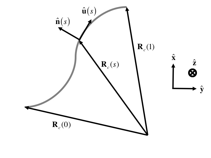
Figure S.1: Geometry for smoothing of discontinuous fields at waveguide interfaces.

We introduce a normal to the curve as

$$\hat{\mathbf{n}}(s) \equiv \hat{\mathbf{z}}\times\hat{\mathbf{u}}(s)$$

$$= \frac{-\hat{\mathbf{y}}\frac{\mathrm{d}x_{c}(s)}{\mathrm{d}s}+\hat{\mathbf{x}}\frac{\mathrm{d}y_{c}(s)}{\mathrm{d}s}}{\sqrt{\left(\frac{\mathrm{d}x_{c}(s)}{\mathrm{d}s}\right)^{2}+\left(\frac{\mathrm{d}y_{c}(s)}{\mathrm{d}s}\right)^{2}}},$$

and in the neighborhood of the curve we can specify the points in the $xy$ plane by $(s,\zeta)$, where

$$\mathbf{R=R}_{c}(s)+\zeta\hat{\mathbf{n}}(s),$$ (S.59)

or

$$x = x_{c}(s)+\zeta\left(\mathbf{\hat{x}\cdot\hat{n}}(s)\right),$$

$$y = y_{c}(s)+\zeta\left(\mathbf{\hat{y}\cdot\hat{n}}(s)\right).$$

For fixed $s$, $\beta_{\text{ref}}$ changes as $\zeta$ passes from $<0$ to $>0$; that is, it is only a function of $\zeta$. We assume now that the change in $\beta_{\text{ref}}(x,y)$ occurs only in such a small region about $\mathbf{R=R}_{c}(s)$ (we will eventually take that change to be a Dirac delta function there) that the mapping from $(\zeta,s)$ to $(x,y)$ is one-to-one. Then we can write

$$\left(\frac{\partial\beta_{\text{ref}}(x,y)}{\partial r^{k}}\right)u_{\alpha q}^{k}(x,y)=\left(\frac{\mathrm{d}\beta_{\text{ref}}(\zeta)}{\mathrm{d}\zeta}\right)\hat{\mathbf{n}}(s)\cdot\mathbf{u}_{\alpha q}(x(s,\zeta),y(s,\zeta)),$$ (S.60)

and we have

$$-\int\mathrm{d}x\mathrm{d}y\,\left(d_{\gamma k}^{i}(x,y)\right)^{*}d_{\gamma{{}^{\prime}}k^{\prime}}^{i}(x,y)\left(\frac{\partial\beta_{\text{ref}}(x,y)}{\partial r^{k}}\right)u_{\alpha q}^{k}(x,y)\\ =-\int\left|J(s,\zeta)\right|\mathrm{d}s\mathrm{d}\zeta\left(d_{\gamma k}^{i}(x,y)\right)^{*}d_{\gamma{{}^{\prime}}k^{\prime}}^{i}(x,y)\left(\frac{d\beta_{\text{ref}}(\zeta)}{d\zeta}\right)\hat{\mathbf{n}}(s)\cdot\mathbf{u}_{\alpha q}(x,y),$$ (S.61)

where in the second line we understand $x=x(s,\zeta)$ and $y=y(s,\zeta)$; that is, we have switched integration variables from $x$ and $y$ to $s$ and $\zeta$. The Jacobian

$$J(s,\zeta)=\left|\begin{array}[]{cc}\frac{\partial x}{\partial s}&\frac{\partial y}{\partial s}\\ \frac{\partial x}{\partial\zeta}&\frac{\partial y}{\partial\zeta}\end{array}\right|=\left(\left(\frac{\mathrm{d}x_{c}(s)}{\mathrm{d}s}+\zeta\hat{\mathbf{x}}\cdot\frac{\partial\hat{\mathbf{n}}(s)}{\mathbf{\partial s}}\right)\hat{\mathbf{y}}\cdot\hat{\mathbf{n}}(s)-\left(\frac{\mathrm{d}y_{c}(s)}{\mathrm{d}s}+\zeta\hat{\mathbf{y}}\cdot\frac{\partial\hat{\mathbf{n}}(s)}{\mathbf{\partial s}}\right)\hat{\mathbf{x}}\cdot\hat{\mathbf{n}}(s)\right).$$ (S.62)

Now at each point $(s,\zeta)$ we can use the local reference frame to identify

$$\left(d_{\gamma k}^{i}(x,y)\right)^{*}d_{\gamma{{}^{\prime}}k^{\prime}}^{i}(x,y)=\left(d_{\gamma k}^{\perp}(x,y)\right)^{*}d_{\gamma^{\prime}k^{\prime}}^{\perp}(x,y)+\left(\mathbf{d}_{\gamma k}^{\parallel}(x,y)\right)^{*}\cdot\mathbf{d}_{\gamma{{}^{\prime}}k^{\prime}}^{\parallel}(x,y),$$ (S.63)

where

$$d_{\gamma{{}^{\prime}}k^{\prime}}^{\perp}(x,y) = \hat{\mathbf{n}}(s)\cdot\mathbf{d}_{\gamma{{}^{\prime}}k^{\prime}}(x,y),$$

$$\mathbf{d}_{\gamma{{}^{\prime}}k^{\prime}}^{\parallel}(x,y) = \mathbf{\hat{z}\hat{z}}\cdot\mathbf{d}_{\gamma{{}^{\prime}}k^{\prime}}(x,y)+\mathbf{\hat{u}}\left(s\right)\mathbf{\hat{u}}\left(s\right)\cdot\mathbf{d}_{\gamma^{\prime}k^{\prime}}(x,y)$$

$$= \mathbf{d}_{\gamma{{}^{\prime}}k^{\prime}}(x,y)-\hat{\mathbf{n}}\left(s\right)\hat{\mathbf{n}}\left(s\right)\cdot\mathbf{d}_{\gamma{{}^{\prime}}k^{\prime}}(x,y),$$

again recalling that $x=x(s,\zeta)$ and $y=y(s,\zeta)$. Then we can write (S.61) as

$$-\int\mathrm{d}x\mathrm{d}y\,\left(d_{\gamma k}^{i}(x,y)\right)^{*}d_{\gamma{{}^{\prime}}k^{\prime}}^{i}(x,y)\left(\frac{\partial\beta_{\text{ref}}(x,y)}{\partial r^{k}}\right)u_{\alpha q}^{k}(x,y)\\ =-\int\left|J(s,\zeta)\right|\mathrm{d}s\mathrm{d}\zeta\left(d_{\gamma k}^{\perp}(x,y)\right)^{*}d_{\gamma{{}^{\prime}}k^{\prime}}^{\perp}(x,y)\left(\frac{\mathrm{d}\beta_{\text{ref}}(\zeta)}{\mathrm{d}\zeta}\right)\hat{\mathbf{n}}(s)\cdot\mathbf{u}_{\alpha q}(x,y)\\ -\int\left|J(s,\zeta)\right|\mathrm{d}s\mathrm{d}\zeta\left(\mathbf{d}_{\gamma k}^{\parallel}(x,y)\right)^{*}\cdot\mathbf{d}_{\gamma^{\prime}k^{\prime}}^{\parallel}(x,y)\left(\frac{\mathrm{d}\beta_{\text{ref}}(\zeta)}{\mathrm{d}\zeta}\right)\hat{\mathbf{n}}(s)\cdot\mathbf{u}_{\alpha q}(x,y).$$ (S.64)

From the relation

$$\varepsilon_{\text{ref}}(\zeta)=\frac{1}{\beta_{\text{ref}}(\zeta)}$$ (S.65)

follows

$$\frac{\mathrm{d}\beta_{\text{ref}}(\zeta)}{\mathrm{d}\zeta}=-\frac{1}{\varepsilon_{\text{ref}}^{2}(\zeta)}\frac{\mathrm{d}\varepsilon_{\text{ref}}(\zeta)}{\mathrm{d}\zeta}.$$ (S.66)

Now the simplest characterization of the variation of $\beta_{\text{ref}}(\zeta)$ would be to write

$$\beta_{\text{ref}}(\zeta)=\beta_{-}+(\beta_{+}-\beta_{-})\theta(\zeta),$$ (S.67)

where $\theta(\zeta)$ is the step function, $\beta_{-}$ is the value of $\beta_{\text{ref}}(\zeta)$ for negative $\zeta$, and $\beta_{+}$ is the value of $\beta_{\text{ref}}(\zeta)$ for positive $\zeta$. Similarly, from (S.65) we can write

$$\varepsilon_{\text{ref}}(\zeta)=\frac{1}{\beta_{-}}+\left(\frac{1}{\beta_{+}}-\frac{1}{\beta_{-}}\right)\theta(\zeta).$$ (S.68)

To differentiate with respect to $\zeta$ and then integrate in (S.64) we smooth these functions. We introduce a smoothing function $g_{l}(\zeta)$ which is non-negative, peaked at $\zeta=0$, satisfies

$$\int g_{l}(\zeta)d\zeta=1,$$ (S.69)

for each $l$, and approaches a Dirac delta function as $l\rightarrow 0$.  Then for finite $l$ we have smoothed functions

$$\bar{\beta}_{\text{ref}}(\zeta) = \int g_{l}(\zeta-\zeta^{\prime})\beta_{\text{ref}}(\zeta^{\prime})\,\mathrm{d}\zeta^{\prime},$$

$$\bar{\varepsilon}_{\text{ref}}(\zeta) = \int g_{l}(\zeta-\zeta^{\prime})\varepsilon_{\text{ref}}(\zeta^{\prime})\,\mathrm{d}\zeta^{\prime}.$$

One strategy for evaluating $\partial\beta_{\text{ref}}(\zeta)/\partial\zeta$ is to take

$$\frac{\mathrm{d}\beta_{\text{ref}}(\zeta)}{\mathrm{d}\zeta}\rightarrow\frac{\mathrm{d}\bar{\beta}_{\text{ref}}(\zeta)}{\mathrm{d}\zeta}=(\beta_{+}-\beta_{-})g_{l}(\zeta).$$ (S.70)

Alternately, using (S.66), we could take

$$\frac{\mathrm{d}\beta_{\text{ref}}(\zeta)}{\mathrm{d}\zeta} \rightarrow -\frac{1}{\bar{\varepsilon}_{\text{ref}}^{2}(\zeta)}\frac{\mathrm{d}\bar{\varepsilon}_{\text{ref}}(\zeta)}{d\zeta}$$

$$= -\frac{1}{\bar{\varepsilon}_{\text{ref}}^{2}(\zeta)}\left(\frac{1}{\beta_{+}}-\frac{1}{\beta_{-}}\right)g_{l}(\zeta).$$

Using (S.70) and (S.IX) in the two right-hand expressions of (S.64) respectively, gives

$$-\int\mathrm{d}x\mathrm{d}y\,\left(d_{\gamma k}^{i}(x,y)\right)^{*}d_{\gamma{{}^{\prime}}k^{\prime}}^{i}(x,y)\left(\frac{\partial\beta_{\text{ref}}(x,y)}{\partial r^{k}}\right)u_{\alpha q}^{k}(x,y)\\ =-(\beta_{+}-\beta_{-})\int\left|J(s,\zeta)\right|\mathrm{d}s\mathrm{d}\zeta\,\left(d_{\gamma k}^{\perp}(x,y)\right)^{*}d_{\gamma{{}^{\prime}}k^{\prime}}^{\perp}(x,y)g_{l}(\zeta)\hat{\mathbf{n}}(s)\cdot\mathbf{u}_{\alpha q}(x,y)\\ +\left(\frac{1}{\beta_{+}}-\frac{1}{\beta_{-}}\right)\int\left|J(s,\zeta)\right|\mathrm{d}s\mathrm{d}\zeta\,\frac{\left(\mathbf{d}_{\gamma k}^{\parallel}(x,y)\right)^{*}\cdot\mathbf{d}_{\gamma{{}^{\prime}}k^{\prime}}^{\parallel}(x,y)}{\bar{\varepsilon}_{\text{ref}}^{2}(\zeta)}g_{l}(\zeta)\hat{\mathbf{n}}(s)\cdot\mathbf{u}_{\alpha q}(x,y),$$ (S.72)

where we still understand $x=x(s,\zeta)$ and $y=y(s,\zeta)$. Now we can let $l\rightarrow 0$ in both terms, because the rest of the integrands are continuous about $\zeta=0$. Recalling (S.69), we have

$$-\int\mathrm{d}x\mathrm{d}y\,\left(d_{\gamma k}^{i}(x,y)\right)^{*}d_{\gamma{{}^{\prime}}k^{\prime}}^{i}(x,y)\left(\frac{\partial\beta_{\text{ref}}(x,y)}{\partial r^{k}}\right)u_{\alpha q}^{k}(x,y)\\ \rightarrow-(\beta_{+}-\beta_{-})\int\left|J(s,0)\right|\left(d_{\gamma k}^{\perp}(\mathbf{R}_{c}(s))\right)^{*}d_{\gamma{{}^{\prime}}k^{\prime}}^{\perp}(\mathbf{R}_{c}(s))\;\hat{\mathbf{n}}(s)\cdot\mathbf{u}_{\alpha q}(\mathbf{R}_{c}(s))\,\mathrm{d}s\\ +\epsilon_{0}^{2}\left(\frac{1}{\beta_{+}}-\frac{1}{\beta_{-}}\right)\int\left|J(s,0)\right|\left(\mathbf{e}_{\gamma k}^{\parallel}(\mathbf{R}_{c}(s))\right)^{*}\cdot\mathbf{e}_{\gamma{{}^{\prime}}k^{\prime}}^{\parallel}(\mathbf{R}_{c}(s))\;\hat{\mathbf{n}}(s)\cdot\mathbf{u}_{\alpha q}(\mathbf{R}_{c}(s))\,\mathrm{d}s.$$ (S.73)

where we have used the fact that $x(s,\zeta)\to x_{c}(s)$, and $y(s,\zeta)\to y_{c}(s)$, as $\zeta\rightarrow 0$. Finally, we have

$$\left|J(s,0)\right|\mathrm{d}s = \left|\left(\frac{\mathrm{d}x_{c}(s)}{\mathrm{d}s}\right)\hat{\mathbf{y}}\cdot\hat{\mathbf{n}}(s)-\left(\frac{\mathrm{d}y_{c}(s)}{\mathrm{d}s}\right)\hat{\mathbf{x}}\cdot\hat{\mathbf{n}}(s)\right|\mathrm{d}s$$

$$= \sqrt{\left(\frac{\mathrm{d}x_{c}(s)}{\mathrm{d}s}\right)^{2}+\left(\frac{\mathrm{d}y_{c}(s)}{\mathrm{d}s}\right)^{2}}\mathrm{d}s=\mathrm{d}R_{c}(s),$$

the element of length along the curve. So we can write

$$-\int\mathrm{d}x\mathrm{d}y\, \left[d_{\gamma k}^{i}(x,y)\right]^{*}d_{\gamma{{}^{\prime}}k^{\prime}}^{i}(x,y)\left(\frac{\partial\beta_{\text{ref}}(x,y)}{\partial r^{k}}\right)u_{\alpha q}^{k}(x,y)$$

$$\rightarrow-(\beta_{+}-\beta_{-})\int\left[d_{\gamma k}^{\perp}(\mathbf{R}_{c}(s))\right]^{*}d_{\gamma{{}^{\prime}}k^{\prime}}^{\perp}(\mathbf{R}_{c}(s))\left[\hat{\mathbf{n}}(s)\cdot\mathbf{u}_{\alpha q}(\mathbf{R}_{c}(s))\right]\,\mathrm{d}R_{c}(s)$$

$$~{}~{}~{}~{}~{}~{}+\epsilon_{0}^{2}\left(\frac{1}{\beta_{+}}-\frac{1}{\beta_{-}}\right)\int\left(\mathbf{e}_{\gamma k}^{\parallel}(\mathbf{R}_{c}(s))\right)^{\ast}\cdot\mathbf{e}_{\gamma{{}^{\prime}}k^{\prime}}^{\parallel}(\mathbf{R}_{c}(s))\left[\hat{\mathbf{n}}(s)\cdot\mathbf{u}_{\alpha q}(\mathbf{R}_{c}(s))\right]\,\mathrm{d}R_{c}(s)$$

$$=(\frac{1}{\varepsilon_{-}}-\frac{1}{\varepsilon_{+}})\int\left(d_{\gamma k}^{\perp}(\mathbf{R}_{c}(s))\right)^{*}d_{\gamma{{}^{\prime}}k^{\prime}}^{\perp}(\mathbf{R}_{c}(s))\left[\hat{\mathbf{n}}(s)\cdot\mathbf{u}_{\alpha q}(\mathbf{R}_{c}(s))\right]\,\mathrm{d}R_{c}(s)$$

$$~{}~{}~{}~{}~{}~{}+\epsilon_{0}^{2}\left(\varepsilon_{+}-\varepsilon_{-}\right)\int\left(\mathbf{e}_{\gamma k}^{\parallel}(\mathbf{R}_{c}(s))\right)^{*}\cdot\mathbf{e}_{\gamma{{}^{\prime}}k^{\prime}}^{\parallel}(\mathbf{R}_{c}(s))\left[\hat{\mathbf{n}}(s)\cdot\mathbf{u}_{\alpha q}(\mathbf{R}_{c}(s))\right]\,\mathrm{d}R_{c}(s),$$ (S.74)

from whence (80) follows. The full expression for $\bar{\Gamma}_{\text{surf}}(\gamma k;\gamma{{}^{\prime}}k^{\prime};\alpha q)$ then involves a sum over all such curves where a transition from one dielectric constant to another occurs. Note there is no ambiguity in evaluating these terms, since $\mathbf{d}_{\gamma k}^{\perp}(\mathbf{r})$ is continuous across a step discontinuity in $\beta_{\text{ref}}(x,y)$, as is $\mathbf{e}_{\gamma{{}^{\prime}}k^{\prime}}^{\parallel}(\mathbf{r}).$

S.X Reduced matrix elements

Using the normalization conditions (29) and (46) we can write the matrix elements in the form

$$\bar{\Gamma}(\gamma k;\gamma{{}^{\prime}}k^{\prime};\alpha q) = \frac{1}{2^{3/2}{\Omega_{\alpha q}}\sqrt{\left|v_{\gamma k}v_{\gamma{{}^{\prime}}k^{\prime}}v_{\alpha q}\right|}}$$

$$\times\left[\frac{\int\mathrm{d}x\mathrm{d}y\,\left(d_{\gamma k}^{i}(x,y)\right)^{*}d_{\gamma^{\prime}k^{\prime}}^{j}(x,y)p^{ijlm}(x,y)S_{\alpha q}^{lm}(x,y)}{\left[\int\mathrm{d}x\mathrm{d}y\,\beta_{\text{ref}}(\mathbf{r})\mathbf{d}_{\gamma k}^{*}(x,y)\cdot\mathbf{d}_{\gamma k}(x,y)\right]\left[\int\mathrm{d}x\mathrm{d}y\,\rho(x,y)\mathbf{u}_{\alpha q}^{\ast}(x,y)\cdot\mathbf{u}_{\alpha q}(x,y)\right]^{1/2}}\right.$$

$$+(\frac{1}{\varepsilon_{-}}-\frac{1}{\varepsilon_{+}})\frac{\int\left(d_{\gamma k}^{\perp}(\mathbf{r}_{c}(s))\right)^{*}d_{\gamma{{}^{\prime}}k^{\prime}}^{\perp}(\mathbf{r}_{c}(s))\left(\hat{\mathbf{n}}(s)\cdot\mathbf{u}_{\alpha q}(\mathbf{r}_{c}(s)\right)dR_{c}(s)}{\left[\int\mathrm{d}x\mathrm{d}y\,\beta_{\text{ref}}(\mathbf{r})\mathbf{d}_{\gamma k}^{*}(x,y)\cdot\mathbf{d}_{\gamma k}(x,y)\right]\left[\int\mathrm{d}x\mathrm{d}y\,\rho(x,y)\mathbf{u}_{\alpha q}^{*}(x,y)\cdot\mathbf{u}_{\alpha q}(x,y)\right]^{1/2}}$$

$$\left.+\left(\varepsilon_{+}-\varepsilon_{-}\right)\frac{\epsilon_{0}^{2}\int\left(\mathbf{e}_{\gamma k}^{\parallel}(\mathbf{r}_{c}(s))\right)^{*}\cdot\mathbf{e}_{\gamma{{}^{\prime}}k^{\prime}}^{\parallel}(\mathbf{r}_{c}(s))\hat{\mathbf{n}}(s)\cdot\mathbf{u}_{\alpha q}(\mathbf{r}_{c}(s))dR_{c}(s)}{\left[\int\mathrm{d}x\mathrm{d}y\,\beta_{\text{ref}}(\mathbf{r})\mathbf{d}_{\gamma k}^{*}(x,y)\cdot\mathbf{d}_{\gamma k}(x,y)\right]\left[\int\mathrm{d}x\mathrm{d}y\,\rho(x,y)\mathbf{u}_{\alpha q}^{*}(x,y)\cdot\mathbf{u}_{\alpha q}(x,y)\right]^{1/2}}\right].$$

The advantage of this form is that it can now be used regardless of how the mode fields are normalized. Again, the last two lines should be summed over all curves that contribute.

S.XI The organization of eigenfunctions

This section establishes the basic properties of partner eigenfunctions for a Hermitian operator that are invoked in section S.III.

Consider a Hermitian operator, schematically $H(x,\frac{\partial}{\partial x},\ldots)$; the eigenvalue equation is

$$H(x,\frac{\partial}{\partial x},\ldots)f(x)=\lambda f(x).$$ (S.76)

Hermiticity guarantees real eigenvalues and the fact that eigenfunctions of different eigenvalues are orthogonal. The inner product of two such functions vanishes, where the inner product of $g(x)$ with $f(x)$ is

$$\int g^{*}(x)f(x)dx$$ (S.77)

We consider eigenfunctions that are normalized, so

$$\int f^{*}(x)f(x)dx=1.$$ (S.78)

We want to consider first a number of degenerate eigenfunctions, all with the same eigenvalue. Suppose now that besides being Hermitian, $H$ is also real. Then if $f(x)$ is an eigenfunction, $f^{*}(x)$ will also be an eigenfunction with the same eigenvalue.

$$H(x,\frac{\partial}{\partial x},\ldots)f^{*}(x)=\lambda f^{*}(x)$$ (S.79)

For a given $f(x)$, of course one possibility is that $f^{*}(x)$ is just a constant phase factor times $f(x)$. Then $f(x)$ could be readjusted to be purely real (or purely imaginary), for example.

Suppose this is not the case. Then $f(x)$ and $f^{*}(x)$ are linearly independent, and they span a two-dimensional space. Of course, they need not be orthogonal. That is, there is no guarantee that the inner product of $f^{*}(x)$ with $f(x)$,

$$\int f(x)f(x)dx$$ (S.80)

vanishes. If it does, we call $f(x)$ and $f^{*}(x)$ “partner” eigenfunctions. Suppose now that (S.80) does not vanish. We can construct partner eigenfunctions from $f(x)$ and $f^{*}(x)$ in the following way.

First find

$$c(x)=N(f(x)+f^{*}(x)),$$ (S.81)

where $N$ is a real normalization constant; $c(x)$ does not vanish, because by assumption $f^{*}(x)$ is not just a multiple of $f(x)$. If we choose $N$ to be real, then $c(x)$ is also purely real. Now take out from $f(x)$ the amount proportional to $c(x)$,

$$\bar{f}(x)=f(x)-c(x)\int c(x^{\prime})f(x^{\prime})dx^{\prime},$$ (S.82)

where we do not need $c^{*}(x^{\prime})$ in the integral because $c(x^{\prime})$ is real. Of course $\bar{f}(x)$ cannot vanish everywhere because otherwise $f(x)$ would just be proportional to $c(x)$ and then $f(x)$ would just be a phase factor times a real function. Now by construction $c(x)$ is orthogonal to $\bar{f}(x),$

$$\int c(x)\bar{f}(x)dx=0.$$ (S.83)

Perhaps $\bar{f}(x)$ is purely real; if so, normalize it and call the result $s(x)$. Perhaps $\bar{f}(x)$ is purely imaginary; if so, divide by $i$, normalize it and call the result $s(x)$. If $\bar{f}(x)$ is neither, note that from (S.83) we have

$$\int c(x)\bar{f}^{*}(x)dx=0,$$ (S.84)

since $c(x)$ is purely real. Then

$$\bar{f}(x)+\bar{f}^{*}(x)$$ (S.85)

is a real function that is orthogonal to $c(x)$; it cannot vanish everywhere because we have assumed that $\bar{f}(x)$ is not purely imaginary. Now normalize this function and call it $s(x)$.

Whatever route we have taken to get $s(x)$, we now have two real functions $c(x)$ and $s(x)$ that are orthogonal to each other and normalized,

$$\int c^{2}(x)dx = 1,$$

$$\int s^{2}(x)dx = 1,$$

$$\int c(x)s(x)dx = 0.$$

They span the space spanned by $f(x)$ and $f^{*}(x)$. We can then form partner functions for this subspace,

$$f_{1}(x) = \frac{1}{\sqrt{2}}(c(x)+is(x)),$$

$$f_{1}^{*}(x) = \frac{1}{\sqrt{2}}(c(x)-is(x)).$$

These functions are normalized,

$$\int\left[f_{1}(x)\right]^{*}f_{1}(x)dx = 1,$$

$$\int\left[f_{1}^{*}(x)\right]^{*}f_{1}^{*}(x)dx = 1,$$

and orthogonal,

$$\int\left[f_{1}^{*}(x)\right]^{*}f_{1}(x)dx = 0,$$

$$\int\left[f_{1}(x)\right]^{*}f_{1}^{*}(x)dx = 0.$$

So we have constructed partner eigenfunctions $f_{1}(x)$ and $f_{1}^{\ast}(x)$ that span the subspace spanned by $f(x)$ and $f^{*}(x)$. Suppose now there are more eigenfunctions with the same eigenvalue, which are orthogonal to $f(x)$ and $f^{*}(x)$. Call one of them $g(x)$. Then $g(x)$ must be orthogonal to $f_{1}(x)$ and $f_{1}^{*}(x)$ since they span the same subspace as $f(x)$ and $f^{*}(x),$

$$\int g^{*}(x)f_{1}(x)dx = 0,$$ (S.86)

$$\int g^{*}(x)f_{1}^{*}(x)dx = 0.$$

Now if $g(x)$ is an eigenfunction of $H(x)$, then $g^{*}(x)$ is an eigenfunction of $H(x)$ with the same eigenvalue. Suppose $g^{*}(x)$ is not just a constant phase factor times $g(x)$; then $g^{*}(x)$ and $g(x)$ span a two dimensional subspace that, since from (S.86) we have immediately

$$\int g(x)f_{1}(x)dx = 0,$$

$$\int g(x)f_{1}^{*}(x)dx = 0,$$

has no overlap with the subspace spanned by $f_{1}(x)$ and $f_{1}^{*}(x)$ . So from $g(x)$ and $g^{*}(x)$ we can form two partner wave functions $f_{2}(x)$ and $f_{2}^{*}(x)$ that are orthogonal to each other and each orthogonal to each of $f_{1}(x)$ and $f_{1}^{*}(x)$.

Thus we can proceed and organize our eigenfunctions. As we investigate all the eigenfunctions of a particular eigenvalue we will sometimes find it is possible to immediately make an eigenfunction real (as we could have, for example, if $g^{*}(x)$ had simply been proportional to $g(x)$ with a constant phase factor), or otherwise we can establish partners. So we can imagine listing all our wave functions grouped in the following manner,

$$f_{1}(x)\;\;f_{1}^{*}(x)$$ (S.87)

$$f_{2}(x)\;\;f_{2}^{*}(x)$$

$$f_{3}(x)\;\;f_{3}^{*}(x)$$

$$\vdots\ \ \ \ \ \ \ \ \vdots$$

$$f_{N}(x)\;\;f_{N}^{*}(x)$$

$$\;\;\;\;\;f_{I}(x)$$

$$\;\;\;\;\;f_{II}(x)$$

$$\;\;\;\;\;\;\vdots$$

Here the Roman numerals indicate real wave functions that “don’t have partners”; we take them to be purely real. Of course, if we have an even number of real wave functions without partners we can start combining them into partners. For example, in the list above we could replace $f_{I}(x)$ and $f_{II}(x)$ by the partners

$$f_{N+1}(x) = \frac{1}{\sqrt{2}}\left(f_{I}(x)+if_{II}(x)\right),$$

$$f_{N+1}^{*}(x) = \frac{1}{\sqrt{2}}\left(f_{I}(x)-if_{II}(x)\right).$$

If we have an even number of eigenfunctions of a particular eigenvalue, then we could pair them all up in partnerships. If we have an odd number then there must be at least one “unpartnered” wave function. It is also possible to “divorce” some partners; for example, in place of $f_{3}(x)$ and $f_{3}^{*}(x)$ we could choose the real functions

$$c_{3}(x) = \frac{1}{\sqrt{2}}\left(f_{3}(x)+f_{3}^{*}(x)\right),$$

$$s_{3}(x) = -\frac{i}{\sqrt{2}}\left(f_{3}(x)-f_{3}^{*}(x)\right).$$

But it is often convenient and natural to have wave functions in partnerships. In any case, we assume that we have eigenfunctions organized according to (S.87). However, we henceforth write $f_{1}^{*}(x)$ as $f_{\bar{1}}(x)$, and so on, so the list (S.87) can be given as

$$f_{1}(x)\;\;f_{\bar{1}}(x)$$ (S.88)

$$f_{2}(x)\;\;f_{\bar{2}}(x)$$

$$f_{3}(x)\;\;f_{\bar{3}}(x)$$

$$\vdots\ \ \ \ \ \ \ \ \vdots$$

$$f_{N}(x)\;\;f_{\bar{N}}(x)$$

$$\;\;\;\;\;f_{I}(x)$$

$$\;\;\;\;\;f_{II}(x)$$

$$\;\;\;\;\;\;\vdots$$

Then if we denote a general eigenfunction by $f_{\alpha}(x)$, the list of possible $Js$ is

$$1,\bar{1},2,\bar{2},3,\bar{3},\ldots N,\bar{N},I,II,III\ldots$$ (S.89)

These eigenfunctions are all orthogonal,

$$\int f_{\alpha}^{*}(x)f_{\alpha^{\prime}}(x)dx=\delta_{\alpha\alpha^{\prime}}.$$ (S.90)

as $\alpha$ and $\alpha^{\prime}$ range over this list. Associated with a list of $\alpha s$ we introduce a list of $\bar{\alpha}s,$

$$\bar{1},1,\bar{2},2,\bar{3},3,\ldots\bar{N},N,I,II,III\ldots$$ (S.91)

That is, if $\alpha$ is one of a partnership, $\bar{\alpha}$ is the other partner; if $\alpha$ is a real wave function, $\bar{\alpha}$ is that wave function itself. Clearly

$$\sum_{\bar{\alpha}}=\sum_{\alpha},$$ (S.92)

and

$$f_{\bar{\alpha}}^{*}(x)=f_{\alpha}(x),$$ (S.93)

either because $\bar{\alpha}$ identifies the partner of $\alpha$, or because $f_{\alpha}(x)$ is real, in which case $f_{\alpha}(x)$ can be considered its own partner.

Now if we consider the eigenfunctions of a whole range of eigenvalues $\lambda$ we can do the same sort of organization within the subspace of each eigenvalue. Then we can let $\alpha$ range over the whole set of labels of all eigenfunctions of all eigenvalues. For a given $\alpha$ we identify the eigenvalue by $\lambda_{\alpha}$. Then over this whole range of $\alpha s$ we have

$$\int f_{\alpha}^{*}(x)f_{\alpha^{\prime}}(x)dx=\delta_{\alpha\alpha^{\prime}},$$ (S.94)

where between eigenfunctions associated with different eigenvalues the orthogonality holds because of Hermiticity of the operator, while between eigenfunctions associated with the same eigenvalue the orthogonality holds because of the construction we have adopted. We still have generally

$$f_{\bar{\alpha}}^{*}(x)=f_{\alpha}(x),$$ (S.95)

and of course

$$\lambda_{\bar{\alpha}}=\lambda_{\alpha}.$$ (S.96)