On the Equivalence among Problems of Bounded Width

Abstract

In this paper, we introduce a methodology, called decomposition-based reductions, for showing the equivalence among various problems of bounded-width.

First, we show that the following are equivalent for any $\alpha>0$:

• SAT can be solved in $O^{*}(2^{\alpha{\bf tw}})$ time,

• 3-SAT can be solved in $O^{*}(2^{\alpha{\bf tw}})$ time,

• Max 2-SAT can be solved in $O^{*}(2^{\alpha{\bf tw}})$ time,

• Independent Set can be solved in $O^{*}(2^{\alpha{\bf tw}})$ time, and

• Independent Set can be solved in $O^{*}(2^{\alpha{\bf cw}})$ time,

where ${\bf tw}$ and ${\bf cw}$ are the tree-width and clique-width of the instance, respectively.

Then, we introduce a new parameterized complexity class EPNL, which includes Set Cover and Directed Hamiltonicity, and show that SAT, 3-SAT, Max 2-SAT, and Independent Set parameterized by path-width are EPNL-complete. This implies that if one of these EPNL-complete problems can be solved in $O^{*}(c^{k})$ time, then any problem in EPNL can be solved in $O^{*}(c^{k})$ time.

1 Introduction

SAT is a fundamental problem in complexity theory. Today, it is widely believed that SAT cannot be solved in polynomial time. This is not only because anyone could not find a polynomial-time algorithm for SAT despite many attempts, but also because if SAT can be solved in polynomial time, any problem in NP can be solved in polynomial time (NP-completeness). Actually, even no algorithms faster than the trivial $O^{*}(2^{n})$-time exhaustive search algorithm are known. Impagliazzo and Paturi [13] conjectured that SAT cannot be solved in $O^{*}((2-\epsilon)^{n})$ time for any $\epsilon>0$, and this conjecture is called the Strong Exponential Time Hypothesis (SETH). Under the SETH, conditional lower bounds for several problems have been obtained, including $k$-Dominating Set [17], problems of bounded tree-width [15, 9], and Edit Distance [3].

When considering polynomial-time tractability, all the NP-complete problems are equivalent, that is, if one of them can be solved in polynomial time, then all of them can be also solved in polynomial time. Similarly, when considering subexponential-time tractability, all the SNP-complete problems are equivalent [14]. However, if we look at the exponential time complexity for solving each NP-complete problem more closely, the situation changes; whereas the current fastest algorithm for SAT is the naive $O^{*}(2^{n})$-time exhaustive search algorithm, faster algorithms have been proposed for many other NP-complete problems such as 3-SAT [12], Max 2-SAT [19], and Independent Set [20]. Although there are many problems, including Set Cover and Directed Hamiltonicity , for which the current fastest algorithms take $O^{*}(2^{n})$ time, we do not know whether a faster algorithm for one of these problems leads to a faster algorithms for SAT and vice versa. Actually, only a few problems, such as Hitting Set and Set Splitting, are known to be equivalent to SAT in terms of exponential time complexity [8].

In this paper, we propose a new methodology, called decomposition-based reductions. Although the idea of decomposition-based reductions is simple, we can obtain various interesting results. First, we show that when parameterized by width, there are many problems that are equivalent to SAT. Second, we show the equivalence among different width; Independent Set parameterized by tree-width and Independent Set parameterized by clique-width are equivalent. Third, we introduce a new parameterized complexity class EPNL, which includes Set Cover and Directed Hamiltonicity, and show that many problems parameterized by path-width are EPNL-complete. For these problems, conditional lower-bounds under the SETH are already known [15]. However, our results imply that these problems are at least as hard as not only $n$-variable SAT but also any problem in EPNL. In this sense, our hardness results are more robust.

It has been shown that many NP-hard graph optimization problems can be solved efficiently if the input graph has a nice decomposition. One of the most famous decompositions is tree-decomposition, and a graph is parameterized by tree-width, the size of the largest bag in the (best) tree-decomposition of the graph. Intuitively speaking, tree-width measures how much a graph looks like a tree. If we are given a graph and its tree-decomposition of width tw , many problems can be solved in $O^{*}(c^{\bf tw})$ time, where $c$ is a problem-dependent constant. For example, we can solve Independent Set and Max 2-SAT in $O^{*}(2^{\bf tw})$ time by standard dynamic programming and Dominating Set in $O^{*}(3^{\bf tw})$ time by combining with subset convolution [18]. Recently, Lokshtanov et al. [15] showed that many of these algorithms are optimal under the SETH. These results are obtained by reducing an $n$-variable instance of SAT to an instance of the target problem with tree-width approximately $\frac{n}{\log c}$, where $c$ is a problem dependent constant. However, these reductions are one-way, and thus a faster SAT algorithm may not lead to faster algorithms for these problems. Moreover, there is a possibility that one of these problems has a faster algorithm but the others do not.

The first contribution of this paper is showing the following equivalence among problems of bounded tree-width:

Theorem 1.

For any $\alpha>0$, the following are equivalent:

1. SAT can be solved in $O^{*}(2^{\alpha{\bf tw}})$ time.

2. 3-SAT can be solved in $O^{*}(2^{\alpha{\bf tw}})$ time.

3. Max 2-SAT can be solved in $O^{*}(2^{\alpha{\bf tw}})$ time.

4. Independent Set can be solved in $O^{*}(2^{\alpha{\bf tw}})$ time.

For all of these problems, the fastest known algorithms run in $O^{*}(2^{\bf tw})$ time [16] and Theorem 1 states that this is not a coincidence. Note that an $n$-variable instance of SAT has tree-width at most $n-1$. Hence by Theorem 1, for any $\epsilon>0$, an $O^{*}((2-\epsilon)^{{\bf tw}})$-time algorithm for Independent Set of bounded tree-width implies an $O^{*}((2-\epsilon)^{n})$-time algorithm for the general SAT. Therefore, our result includes the hardness result by Lokshtanov et al. [15]. We believe that the same technique can be applied to many other problems. In practice, SAT solvers are widely used to solve various problems by reductions to SAT. Using our methodology, we can reduce an instance of some problem to an instance of SAT by preserving the tree-width. Since tree-decompositions can be used to speed-up SAT solvers [11], our reductions may be useful in practice.

Clique-width is the number of labels we need to construct the given graph by iteratively performing certain operations. Similarly to the tree-width case, many problems can be solved in $O^{*}(c^{\bf cw})$ time if the given graph has a clique-width ${\bf cw}$, where $c$ is a problem-dependent constant [7].

The second contribution of this paper is showing the following equivalence between Independent Set of bounded tree-width and bounded clique-width:

Theorem 2.

For any $\alpha>0$, the following are equivalent:

1. Independent Set can be solved in $O^{*}(2^{\alpha{\bf tw}})$ time.

2. Independent Set can be solved in $O^{*}(2^{\alpha{\bf cw}})$ time.

The fastest known algorithms for Independent Set parameterized by clique-width runs in $O^{*}(2^{\bf cw})$ time [7]. It is surprising that we can obtain such strong connections between problems of bounded tree-width and a problem of bounded clique-width because tree-width and clique-width are very different parameters in nature; a complete graph of $n$ vertices has a clique-width two whereas its tree-width is $n-1$. Hence, even if there is an efficient algorithm for a problem of bounded tree-width, it does not immediately imply that there is an efficient algorithm for the same problem of bounded clique-width. However, Theorem 2 states that a faster algorithm for Independent Set of bounded tree-width implies a faster algorithm for Independent Set of bounded clique-width. We note that Independent Set is chosen because SAT, 3-SAT, and Max 2-SAT are still NP-complete when its primal graph is a clique (${\bf cw}=2$). Hence, these problems parameterized by tree-width and clique-width are not equivalent unless $\mbox{{P}}=\mbox{{NP}}$. We believe that we can obtain similar results for many other problems that can be solved efficiently on graphs of bounded clique-width.

The third contribution of this paper is introducing a new parameterized complexity class EPNL (Exactly Parameterized NL) and showing the following complete problems:

Theorem 3.

SAT, 3-SAT, Max 2-SAT, and Independent Set parameterized by path-width are EPNL-complete.

Intuitively, EPNL is a class of parameterized problems that can be solved by a non-deterministic Turing machine with the space of $k+O(\log n)$ bits. For the precise definitions of EPNL and EPNL-completeness, see Section 9. Flum and Grohe [10] introduced a similar class, called para-NL, that can be solved in $f(k)+O(\log n)$ space. Although they showed that a trivial parameterization of an NL-complete problem is para-NL-complete under the standard parameterized reduction, this does not hold in our case because we use a different reduction to define the complete problems. If one of the NP-complete problems can be solved in polynomial time, any problem in NP can be solved in polynomial time. Similarly, if one of the EPNL-complete problems can be solved in $O^{*}(c^{k})$ time, any problem in EPNL can be solved in $O^{*}(c^{k})$ time. Since the class EPNL contains many famous problems, such as Set Cover parameterized by the number of elements and Directed Hamiltonicity parameterized by the number of vertices, for which no $O^{*}((2-\epsilon)^{n})$-time algorithms are known, our result implies that we can use the hardness of not only SAT but also these problems to establish the hardness of the problems parameterized by path-width.

1.1 Overview of Decomposition-based Reductions

We explain the basic idea of decomposition-based reductions. Although we deal with three different decompositions in this paper, the basic idea is the same. We believe that the same idea can be used to other decompositions such as branch-decomposition.

A decomposition can be seen as a collection of sets forming a tree. For example, tree-decomposition is a collection of bags forming a tree and clique-decomposition is a collection of labels forming a tree. First, for each node $i$ of a decomposition tree, we create gadgets as follows: (1) for each element $x$ in the corresponding set $X_{i}$, create a path-like gadget $x_{i}$ that expresses the state of the element (e.g. the value of the variable $x$ for the case of SAT), and (2) create several gadgets to solve subproblem corresponding to this node (e.g. simulate clauses inside $X_{i}$ for the case of SAT). Then, for each node $c$, its parent $p$, and each common element $x\in X_{c}\cap X_{p}$, by connecting the tail of $x_{c}$ and the head of $x_{p}$, we establish local consistency. From the definition of the decomposition, this leads to global consistency. Since the obtained graph has a locality, it has a small width. We may need additional tricks to establish local consistency without increasing the width.

1.2 Organization

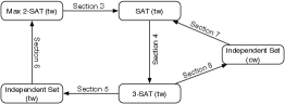
Figure 1: Reductions given in this paper

The rest of the paper is organized as follows. In Section 2, we introduce definitions and basic lemmas often used in this paper. In Section 3, we give a tree-width preserving reduction from Max 2-SAT to SAT. The reduction is rather simple but contains an essential idea of tree-decomposition-based reductions. The other reductions are given in Sections 4 - 8 (see Figure 1). In Section 9, we introduce EPNL and show that SAT parameterized by path-width is EPNL-complete.

2 Preliminaries

For an integer $k$, we denote the set $\{1,2,\ldots,k\}$ by $[k]$ and the set $\{0,1,\ldots,k-1\}$ by $[k]^{\prime}$. Let $G=(V,E)$ be an undirected graph. We denote the degree of a vertex $v$ as $d_{G}(v)$. We denote the neighborhood of a vertex $u$ by $N_{G}(u)=\{v\in V\mid\{u,v\}\in E\}$, and the closed neighborhood of $u$ by $N_{G}[u]=N_{G}(u)\cup\{u\}$. Similarly, we denote the neighborhood of a subset $S\subseteq V$ by $N_{G}(S)=\bigcup_{v\in S}N_{G}(v)\setminus S$, and the closed neighborhood by $N_{G}[S]=N_{G}(S)\cup S$. We drop the subscript $G$ when it is clear from the context. For a subset $S\subseteq V$, let $G[S]=(S,\{\{u,v\}\in E\mid u\in S,v\in S\})$ denote the subgraph induced by $S$. For a vertex $v\in V$, let $G/v$ denote the graph obtained by removing $v$ and making the neighbors of $v$ form a clique. We call this operation eliminating $v$. Similarly, for a subset $S\subseteq V$, we denote by $G/S$ the graph obtained by removing $S$ and making the neighbors of $S$ form a clique.

A tree-decomposition of a graph $G=(V,E)$ is a pair $(T,\chi)$, where $T=(I,F)$ is a tree and $\chi=\{X_{i}\subseteq V\mid i\in I\}$ is a collection of subsets of vertices (called bags), with the following properties:

1. $\bigcup_{i}X_{i}=V$.

2. For each edge $uv\in E$, there exists a bag that contains both of $u$ and $v$.

3. For each vertex $v\in V$, the bags containing $v$ form a connected subtree in $T$.

In order to avoid confusion between a graph and its decomposition tree $T$, we call a vertex of the tree a node, and an edge of the tree an arc. We identify a node $i\in I$ of the tree and the corresponding bag $X_{i}$. The width of a tree-decomposition is the maximum of $|X_{i}|-1$ over all nodes $i\in I$. The tree-width of a graph $G$, ${\bf tw}(G)$, is the minimum width among all the possible tree-decompositions of $G$.

A nice tree-decomposition is a tree decomposition such that the root bag $X_{r}$ is an empty set and each node $i$ is one of the following types:

1. Leaf: a leaf node with $X_{i}=\emptyset$.

2. Introduce($v$): a node with one child $c$ such that $X_{i}=X_{c}\cup\{v\}$ and $v\not\in X_{c}$.

3. Introduce($uv$): a node with one child $c$ such that $u,v\in X_{i}=X_{c}$. We require that this node appears exactly once for each edge $uv$ of $G$.

4. Forget($v$): a node with one child $c$ such that $X_{i}=X_{c}\setminus\{v\}$ and $v\in X_{c}$. From the definition of tree-decompositions, this node appears exactly once for each vertex of $G$.

5. Join: a node with two children $l$ and $r$ with $X_{i}=X_{l}=X_{r}$.

Any tree-decomposition can be easily converted into a nice tree-decomposition of the same width in polynomial time by inserting intermediate bags between each adjacent bags. Thus, in this paper, we use nice tree-decompositions to make discussions simple.

A (nice) path-decomposition is a (nice) tree-decomposition $(T,\chi)$ such that the decomposition tree $T=(I,F)$ is a path. The path-width of a graph $G$, ${\bf pw}(G)$, is the minimum width among all the possible path-decompositions of $G$.

In order to prove the upper bound on tree-width, we will often use the following lemmas.

Lemma 1 (Arnborg [1]).

For a graph $G=(V,E)$ and a vertex $v\in V$, ${\bf tw}(G)\leq\max(d(v),{\bf tw}(G/v))$. Moreover, if we are given a tree-decomposition of $G/v$ of width $w$, we can construct a tree-decomposition of $G$ of width $\max(d(v),w)$ in linear time.

Proof.

Let $T=(I,F)$ be a tree-decomposition of $G/v$ of width $w$. Since the neighbors $N(v)$ form a clique in $G/v$, there exists a node $i\in I$ such that the bag $X_{i}$ contains $N(v)$. Therefore, by creating a node $j$ with $X_{j}=N[v]$ and adding an arc $ij$, we can obtain a tree-decomposition of $G$. The width of this tree-decomposition is $\max(|X_{j}|-1,w)=\max(d(v),w)$. ∎

Lemma 2.

For a graph $G=(V,E)$ and a vertex subset $S\subseteq V$, ${\bf tw}(G)\leq\max(|N[S]|-1,{\bf tw}(G/S))$.

Proof.

Let $S=\{v_{1},...,v_{k}\}$. We eliminate each vertex of $S$ one by one. We denote the graph after the $i$-th elimination by $G_{i}=((G/v_{1})/v_{2})\ldots/v_{i}$. By eliminating $v_{i}$ from $G_{i-1}$, we obtain ${\bf tw}(G_{i-1})\leq\max(d_{G_{i-1}}(v_{i}),{\bf tw}(G_{i}))$. Since $N_{G_{i-1}}(v_{i})\subseteq N_{G}[S]\setminus\{v_{i}\}$, we have ${\bf tw}(G)={\bf tw}(G_{0})\leq\max(|N[S]|-1,{\bf tw}(G_{k}))$. Because $G_{k}$ is a subgraph of $G/S$ and any tree-decomposition of a graph is also a tree-decomposition of its subgraph, we obtain ${\bf tw}(G)\leq\max(|N[S]|-1,{\bf tw}(G/S))$. ∎

Lemma 3.

Let $X$ and $Y$ be disjoint vertex sets of a graph $G$ such that for each vertex $x\in X$, $|N(x)\cap Y|\leq 1$. Then, ${\bf tw}(G)\leq\max(|N[X]\setminus Y|,{\bf tw}(G/X))$.

Proof.

Let $X=\{x_{i}\mid i\in[k]\}$ and $U=N(X)\setminus Y$. For an integer $i$, we denote the vertex set $\{x_{j}\mid j\in[i]\}$ by $X_{i}$. We eliminate each vertex of $X$ one by one. After eliminating vertices $X_{i-1}$, $x_{i}$ can be adjacent only to vertices in $(X\setminus X_{i})\cup\{Y\cap N(X_{i})\}\cup U$. Since $|Y\cap N(X_{i})|\leq i$, we have $d(x_{i})\leq|X|-i+i+|U|=|X|+|U|=|N[X]\setminus Y|$. By iteratively applying Lemma 1, we obtain ${\bf tw}(G)\leq\max(|N[X]\setminus Y|,{\bf tw}(G/X))$. ∎

Lemma 4.

Let $\{S_{i}\mid i\in[d]\}$ be a family of disjoint vertex sets of a graph $G$ such that each set has size at most $k$ and there are no edges between $S_{i}$ and $S_{j}$ for any $|i-j|>1$. Then, ${\bf tw}(G)\leq\max(2k+|N(S)|-1,{\bf tw}(G/S))$, where $S=\bigcup_{i\in[d]}S_{i}$.

Proof.

Let $U=N(S)$. We eliminate each vertex set $S_{i}$ one by one. After eliminating vertex sets $\{S_{j}\mid j\in[i-1]\}$, it holds that $N(S_{i})\subseteq S_{i+1}\cup U$. Thus, we have $|N[S_{i}]|\leq 2k+|U|$. By iteratively applying Lemma 2, we obtain ${\bf tw}(G)\leq\max(2k+|N(S)|-1,{\bf tw}(G/S))$. ∎

For a vertex set $S$, if we can obtain ${\bf tw}(G)\leq\max(d,{\bf tw}(G/S))$ by applying one of these lemmas, we say that the elimination has degree $d$. If we can reduce a graph $G$ into a graph $G^{\prime}$ by a series of eliminations of degree at most $d$, we can obtain ${\bf tw}(G)\leq\max(d,{\bf tw}(G^{\prime}))$.

Let $x$ be a Boolean variable. We denote the negation of $x$ by $\overline{x}$. A literal is either a variable or its negation, and a clause is a disjunction of several literals $l_{1},\dots,l_{k}$, where $k$ is called the length of the clause. We call a clause of length $k$ a $k$-clause. A CNF is a conjunction of clauses. If all the clauses have length at most $k$, it is called a k-CNF. We say that a CNF on a variable set $X$ is satisfiable if there is an assignment to $X$ that makes the CNF true. ($k$-)SAT is a problem in which, given a variable set $X$ and a ($k$-)CNF ${\mathcal{C}}$, the objective is to determine whether ${\mathcal{C}}$ is satisfiable or not. Max 2-SAT is a problem in which, given a variable set $X$, a 2-CNF ${\mathcal{C}}$, and an integer $k$, the objective is to determine whether there exists an assignment that satisfies at least $k$ clauses in ${\mathcal{C}}$.

Let ${\mathcal{C}}$ be a CNF on variables $X$. The primal graph of ${\mathcal{C}}$ is the graph $G=(X,E)$ such that there exists an edge between two vertices if and only if their corresponding variables appear in the same clause. For readability, we identify a variable or a literal as the corresponding vertex in the primal graph. That is, we may use the same symbol $x$ to indicate both a variable in a CNF and the corresponding vertex in the primal graph, and both literals $x$ and $\overline{x}$ correspond to the identical vertex in the primal graph. For a CNF ${\mathcal{C}}$, we slightly change the definition of the nice tree-decomposition as follows:

1. Introduce($C$): an internal node with one child $c$ such that $X_{i}=X_{c}$ and all the variables in $C$ are in $X_{i}$. We require that this node appears exactly once for each clause $C\in{\mathcal{C}}$.

Note that because the variables in the same clause form a clique in the primal graph, there always exists a bag that contains all of them.

In our reductions, we will use a binary representation of an integer. Let $\{a_{1},a_{2},\ldots,a_{M}\}$ be Boolean variables. We denote the integer $\sum_{i\in[M],a_{i}=\mathrm{true}}2^{i-1}$ by $(a_{1}a_{2}\ldots a_{M})_{2}$, or $(a_{*})_{2}$ for short. For readability, we will frequently use (arithmetic) constraints such as $(a_{*})_{2}=(b_{*})_{2}+(c_{*})_{2}$. Note that any arithmetic constraint on $M$ variables can be trivially simulated by at most $2^{M}$ $M$-clauses. Thus, if $M$ is logarithmic in the input size, the number of required clauses is polynomial in the input size.

3 Tree-width preserving reduction from Max 2-SAT to SAT

Let $(X,{\mathcal{C}}=\{C_{1},\ldots,C_{m}\},k)$ be an instance of Max 2-SAT. We want to construct an instance $(X^{\prime},{\mathcal{C}}^{\prime})$ of SAT such that ${\mathcal{C}}^{\prime}$ is satisfiable if and only if at least $k$ clauses of ${\mathcal{C}}$ can be satisfied. Let $M=\left\lceil\log{(m+1)}\right\rceil$. In the following reductions, we will use arithmetic constraints on $O(M)$ variables, which can be simulated by $\mathrm{poly}(m)$ clauses.

Let $T=(I,F)$ be a given nice tree-decomposition of width ${\bf tw}$. We will create an instance of SAT whose tree-width is at most ${\bf tw}+O(\log m)$. We note that the additive $O(\log m)$ factor is allowed because $O^{*}(2^{\alpha({\bf tw}+O(\log m))})=O^{*}(2^{\alpha{\bf tw}}\mathrm{poly}(m))=O^{*}(2^{\alpha{\bf tw}})$. For each node $i\in I$, we create variables $\{x_{i}\mid x\in X_{i}\}\cup\{s_{i,j}\mid j\in[M]\}\cup\{w_{i}\}$. The value $(s_{i,*})_{2}$ will represent the number of satisfied clauses in the subtree rooted at $i$. For each node $i$ and its parent $p$, we create a constraint $x_{i}=x_{p}$ for each variable $x\in X_{i}\cap X_{p}$. Because the nodes containing the same variable form a connected subtree in $T$, these constraints ensure that for any variable $x\in X$, all the variables $\{x_{i}\mid x\in X_{i}\}$ take the same value. For each node $i$, according to its type, we do as follows:

1. Leaf: create a clause $(\overline{s_{i,j}})$ for each $j\in[M]$.

2. Introduce($v$): create a constraint $s_{i,j}=s_{c,j}$ for each $j\in[M]$.

3. Introduce($x\vee y$): create a constraint $w_{i}\Leftrightarrow(x_{i}\vee y_{i})$ and a constraint $(s_{i,*})_{2}=(s_{c,*})_{2}+(w_{i})_{2}$.

4. Forget($v$): create a constraint $s_{i,j}=s_{c,j}$ for each $j\in[M]$.

5. Join: create a constraint $(s_{i,*})_{2}=(s_{l,*})_{2}+(s_{r,*})_{2}$.

Finally for the root node $r$, we create a constraint $(s_{r,*})_{2}\geq k$. Now, we have obtained an instance $(X^{\prime},{\mathcal{C}}^{\prime})$ of polynomial size. We note that, from the definition of a nice tree-decomposition, there exists exactly one Introduce($C$) node for each clause $C\in{\mathcal{C}}$. Thus, the sum $\sum_{i\in I}(w_{i})_{2}$, which is equal to $(s_{r,*})_{2}$, represents the number of satisfied clauses. Therefore, ${\mathcal{C}}^{\prime}$ is satisfiable if and only if at least $k$ clauses of ${\mathcal{C}}$ can be satisfied. Finally, we show that the reduction preserves the tree-width.

Lemma 5.

${\mathcal{C}}^{\prime}$ has tree-width at most ${\bf tw}+O(\log m)$.

Proof.

We will prove the bound by reducing the primal graph of ${\mathcal{C}}^{\prime}$ into an empty graph by a series of eliminations of degree at most ${\bf tw}+O(\log m)$. For a node $i$, let $Y_{i}$ denote the vertex set $\{x_{i}\mid x\in X_{i}\}$ and $V_{i}$ denote the vertex set $Y_{i}\cup\{w_{i}\}\cup\{s_{i,j}\mid j\in[M]\}$. Starting from the primal graph of ${\mathcal{C}}^{\prime}$ and the given tree-decomposition $T$ of ${\mathcal{C}}$, we eliminate the vertices as follows. First, we choose an arbitrary leaf $i$ of $T$. Then, we eliminate all the vertices of $V_{i}$ in a certain order, which will be described later. Finally, we remove $i$ from $T$ and repeat the process until $T$ becomes empty.

Let $i$ be a leaf and $p$ be its parent. If $i$ is the only child of $p$, we have $N(V_{i})\subseteq V_{p}$. Thus, the eliminations of $V_{i}$ can create edges only inside $V_{p}$. If $p$ has another child $q$, we have $N(V_{i})\subseteq V_{p}\cup\{s_{q,j}\mid j\in[M]\}$. Thus, the eliminations of $V_{i}$ can create edges only inside $V_{p}\cup\{s_{q,j}\mid j\in[M]\}$. Therefore, after processing each node, we can ensure that the edges created by previous eliminations are only inside $V_{i}\cup\{s_{c,j}\mid c\text{ is a child of }i\text{ and }j\in[M]\}$ for each node $i$.

Now, we describe the details of the eliminations. Let $i$ be the current node to process. If $i$ is the root, the number of remaining vertices is $O(\log m)$. Thus, the elimination of these vertices has degree $O(\log m)$. Otherwise, let $p$ be the parent of $i$. First, we eliminate the vertices $Y_{i}$. Because each vertex of $Y_{i}$ is adjacent to at most one vertex of $Y_{p}$, Lemma 3 gives the elimination of degree $|N[Y_{i}]\setminus Y_{p}|\leq|V_{i}|\leq{\bf tw}+O(\log m)$. Then, we eliminate the remaining vertices $V_{i}\setminus Y_{i}$. If $i$ is the only child of $p$, let $V_{q}=Y_{q}=\emptyset$, and otherwise, let $q$ be the another child of $p$. By applying Lemma 2, we obtain the elimination of degree $|N[V_{i}\setminus Y_{i}]|-1\leq|V_{i}\setminus Y_{i}|+|V_{p}|+|V_{q}\setminus Y_{q}|\leq{\bf tw}+O(\log m)$. ∎

4 Tree-width preserving reduction from SAT to 3-SAT

Let $(X,{\mathcal{C}}=\{C_{1},\ldots,C_{m}\})$ be an instance of SAT and ${\bf tw}$ be its tree-width. We can use the standard reduction from SAT to 3-SAT: replacing each clause $(x_{1}\vee\ldots\vee x_{k})$ with clauses $(x_{1}\vee x_{2}\vee y_{1}),(\overline{y_{1}}\vee x_{3}\vee y_{2}),\ldots,(\overline{y_{k-3}}\vee x_{k-1}\vee x_{k})$.

Now, we show that the tree-width of the obtained 3-CNF is at most ${\bf tw}+2$. For each clause $(x_{1}\vee\ldots\vee x_{k})$ of the original CNF, we have created $k-3$ new variables $Y=\{y_{1},y_{2},\ldots,y_{k-3}\}$. Let $S_{i}=\{y_{i}\}$ for $i\in[k-3]$. Since there is no edge between $S_{i}$ and $S_{j}$ for $|i-j|>1$, from Lemma 4, we obtain the elimination of $Y$ of degree $2\times 1+|N(S)|-1=k+1$. Since variables in the same clause form a clique in the primal graph, we have ${\bf tw}\geq k-1$. Thus, the elimination has degree at most ${\bf tw}+2$. After applying the above elimination to all the clauses, the graph coincides with the primal graph of ${\mathcal{C}}$. Therefore, the tree-width of the obtained 3-CNF is at most ${\bf tw}+2$.

5 Tree-width preserving reduction from 3-SAT to Independent Set

An independent set of a graph $G=(V,E)$ is a set $S\subseteq V$ such that $G[S]$ has no edges. Independent Set is the problem in which, given a graph $G$ and an integer $k$, the objective is to determine whether there exists an independent set of $G$ with size at least $k$.

Let $(X,{\mathcal{C}}=\{C_{1},\ldots,C_{m}\})$ be an instance of 3-SAT. We want to construct an instance $(G,k)$ of Independent Set with essentially the same tree-width such that $G$ has an independent set of size at least $k$ if and only if ${\mathcal{C}}$ is satisfiable. Actually, in our reductions, we choose $k$ so that any independent set has size at most $k$. In the following reductions, we will use two gadgets depicted in Figure 2.

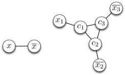
Figure 2: The variable gadget for a variable $x$ and the clause gadget for a clause $(\overline{x_{1}}\vee x_{2}\vee x_{3})$

A variable gadget of a variable $x$ consists of two vertices $x$ and $\overline{x}$ connected by an edge. Any independent set can contain at most one of $x$ and $\overline{x}$. By choosing $k$ properly, we ensure that any independent set of size $k$ contains exactly one of them. This gadget will represent whether a variable $x$ is assigned true (the vertex $x$ is in the independent set) or false (the vertex $\overline{x}$ is in the independent set).

A clause gadget of a clause $C=(x_{1}\vee x_{2}\vee\ldots\vee x_{d})$ consists of $d$ vertices $\{c_{i}\mid i\in[d]\}$ forming a clique ($x_{1},\ldots,x_{d}$ are literals rather than variables). By choosing $k$ properly, we ensure that any independent set of size $k$ contains exactly one of them. We call the operation of creating a clique $\{c_{i}\mid i\in[d]\}$ and inserting edges $\{c_{i}\overline{x_{i}}\mid i\in[d]\}$ creating a clause gadget $C$. If an independent set contains one vertex from the clause gadget, at least one of the vertices $\{\overline{x_{i}}\mid i\in[d]\}$ are not in the independent set. By our choice of $k$, we ensure that at least one of $\{x_{i}\mid i\in[d]\}$ must be in the independent set. Therefore, it acts as a clause $C$.

First, we explain a naive reduction from 3-SAT to Independent Set that does not preserve tree-width. For each variable $x\in X$, we create a corresponding variable gadget, and for each clause $(x\vee y\vee z)\in{\mathcal{C}}$, we create a corresponding clause gadget. Finally, we set $k$ as the number of variable gadgets plus the number of clause gadgets. Now, we have obtained an instance $(G,k)$ of Independent Set. From our choice of $k$, if $G$ contains an independent set of size $k$, it must contain exactly one vertex from each variable gadget and clause gadget. Therefore ${\mathcal{C}}$ is satisfiable. Conversely, if ${\mathcal{C}}$ is satisfiable, we can construct an independent set of size $k$ by choosing an appropriate vertex from each gadget.

Let ${\bf tw}$ be the tree-width of ${\mathcal{C}}$. We omit the proof but the above naive reduction increases the tree-width of $G$ to $2{\bf tw}+O(1)$. This is because, instead of a single variable $x$, we need to keep two vertices $x$ and $\overline{x}$ of the variable gadget in a bag. Intuitively, in order to preserve tree-width, we can put only one of $x$ and $\overline{x}$ in a bag. Our solution is forgetting and remembering the state of $x$ and $\overline{x}$ along the tree-decomposition.

Now, we explain our tree-decomposition-based reduction. Let $M=\left\lceil\log{({\bf tw}+2)}\right\rceil$. We will construct a graph with tree-width at most ${\bf tw}+O(\log{\bf tw})$. As we discussed before, the additive $O(\log{\bf tw})$ factor is allowed. Let $T=(I,F)$ be a given nice tree-decomposition of width ${\bf tw}$. For each node $i\in I$, we create a variable gadget for each of $\{x_{i}\mid x\in X_{i}\}$. If $i$ is an Introduce($x\vee y\vee z$) node, we create a clause gadget for $(x_{i}\vee y_{i}\vee z_{i})$. If $i$ is not the root, let $p$ be its parent and $P_{i}$ be the set $X_{i}\cap X_{p}$. Then, for each $x\in P_{i}$, we connect $\overline{x_{i}}$ and $x_{p}$ by an edge. We want to ensure that for any independent set $S$ of size $k$, $x_{i}$ is in $S$ if and only if $x_{p}$ is in $S$. If $\overline{x_{i}}$ is in $S$, $x_{p}$ cannot be in $S$, and therefore $\overline{x_{p}}$ must be in $S$. On the other hand, even if $x_{i}$ is in $S$, $\overline{x_{p}}$ can be in $S$. In order to avoid such a situation, we will create a gadget to count the number of vertices in $(\{x_{i}\mid x\in P_{i}\}\cup\{\overline{x_{p}}\mid x\in P_{i}\})\cap S$ (this is the most interesting part of our reduction). Because $x_{i}\not\in S$ implies $\overline{x_{p}}\in S$, the number is always at least $|P_{i}|$, and if (and only if) the number is exactly $|P_{i}|$, it holds that $x_{i}\in S\Leftrightarrow x_{p}\in S$ for any $x\in P_{i}$. Since the nodes containing the same variable form a connected subtree, this ensures that for any independent set of size $k$ and for any variable $x$, all the vertices $\{x_{i}\mid x\in X_{i}\}$ are in $S$ or none of them are in $S$. By using the binary encoding, the number can be expressed by $O(\log{\bf tw})$ variables. Thus, we can make the gadget to increase the tree-width only by $O(\log{\bf tw})$.

We will construct such a gadget by using the following gadget. Let $U=\{u_{1},\ldots,u_{d}\}$ be a set of vertices. A counting gadget of $U$ consists of the following $d+1$ layers of variable gadgets connected by clause gadgets. For each $a\in[d]$, the $a$-th layer consists of a variable gadget for $y_{a}$ and variable gadgets for each of $\{s_{a,j}\mid j\in[M]\}$. The last layer consists of variable gadgets for each of $\{s_{d+1,j}\mid j\in[M]\}$. Then, for each $j\in[M]$, we create a clause gadget for $(\overline{s_{1,j}})$, and for each $a\in[d]$, we create clause gadgets simulating an arithmetic constraint $(s_{a+1,*})_{2}=(s_{a,*})_{2}+(y_{a})_{2}$. Finally, for each $a\in[d]$, we connect $u_{a}$ and $\overline{y_{a}}$ by an edge. For an independent set $S$, the number $(s_{d+1,*})_{2}$ in the last layer represents the size of $\{y_{a}\mid a\in[d]\}\cap S$. Since $u_{a}\in S$ implies $y_{a}\in S$, the number is at least the size of $U\cap S$.

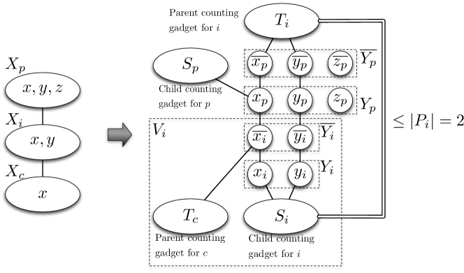
Figure 3: Reduction from 3-SAT to Independent Set

Now, we construct the gadget (see Figure 3). First, we construct a counting gadget for the set $\{x_{i}\mid x\in P_{i}\}$, called a child counting gadget for $i$. Then, we construct a counting gadget for the set $\{\overline{x_{p}}\mid x\in P_{i}\}$, called a parent counting gadget for $i$. Finally, we create clause gadgets simulating the arithmetic constraint that the sum of the numbers represented by the last layers of these two counting gadgets must be at most $|P_{i}|$. As we discussed before, the size $|(\{x_{i}\mid x\in P_{i}\}\cup\{\overline{x_{p}}\mid x\in P_{i}\})\cap S|$ is always at least $|P_{i}|$ and becomes exactly $|P_{i}|$ if and only if $x_{i}\in S\Leftrightarrow x_{p}\in S$ holds for any $x\in P_{i}$. Since the sum is at least the size $|(\{x_{i}\mid x\in P_{i}\}\cup\{\overline{x_{p}}\mid x\in P_{i}\})\cap S|$, the constraint that the sum is at most $|P_{i}|$ implies that $x_{i}\in S\Leftrightarrow x_{p}\in S$ for any $x\in P_{i}$.

Now, we have obtained a graph $G$ of polynomial size and we set $k$ as the number of variable gadgets plus the number of clause gadgets. From our construction, for any independent set $S$ of size $k$ and a variable $x\in X$, all the vertices $\{x_{i}\mid i\in I\text{ s.t. }x\in X_{i}\}$ are in $S$ or none of them are in $S$. Thus, if $G$ has an independent set of size $k$, ${\mathcal{C}}$ is satisfiable. Conversely, if ${\mathcal{C}}$ is satisfiable, by taking an appropriate vertex from each gadget, we can obtain an independent set of size $k$. Finally, we show that the reduction preserves the tree-width.

Lemma 6.

$G$ has tree-width at most ${\bf tw}+O(\log{\bf tw})$.

Proof.

We will prove the bound by reducing $G$ into an empty graph by a series of eliminations of degree at most ${\bf tw}+O(\log{\bf tw})$. Starting from $G$ and the given tree-decomposition $T$ of ${\mathcal{C}}$, we eliminate the vertices as follows.

First, for each clause gadget other than the clause gadgets for $C\in{\mathcal{C}}$ (created when processing the Introduce($C$) node), we eliminate its vertices $S$. Since the size of $N[S]$ is $O(\log{\bf tw})$ and no two vertices in different clause gadgets are adjacent, from Lemma 2, we obtain eliminations of degree $O(\log{\bf tw})$.

For a node $i\in I$, let $Y_{i}$ and $\overline{Y_{i}}$ denote the vertex sets $\{x_{i}\mid x\in X_{i}\}$ and $\{\overline{x_{i}}\mid x\in X_{i}\}$, respectively. If $i$ is an Introduce node, then let $C_{i}$ denote the set of vertices in the corresponding clause gadget, and otherwise, let $C_{i}$ be an empty set. If $i$ is not the root and has a parent $p$, let $S_{i,a}$ be the set of vertices in the variable gadgets of the $a$-th layer of the child counting gadget for $i$. If $i$ is the root, we set $S_{i,a}$ as an empty set. We denote the set of all the vertices of the child counting gadget by $S_{i}=\bigcup_{a\in[d+1]}S_{i,a}$, where $d=|X_{i}\cap X_{p}|$. Similarly, let $T_{i,a}$ be the set of vertices in the variable gadgets of the $a$-th layer of the parent counting gadget for $i$ and $T_{i}=\bigcup_{a\in[d+1]}T_{i,a}$. Let $V_{i}$ denote the union of $Y_{i}$, $\overline{Y_{i}}$, $C_{i}$, $S_{i}$, and $T_{c}$ for each child $c$ of $i$. Now, we eliminate each $V_{i}$ as follows.

First, we choose an arbitrary leaf $i$ of the tree $T$. Then, we eliminate all the vertices of $V_{i}$ in a certain order, which will be described later. Finally, we remove $i$ from $T$ and repeat the process until $T$ becomes empty.

Since $N(V_{i})\subseteq Y_{p}\cup T_{i,d+1}$ holds for a leaf $i$ and its parent $p$, where $d=|X_{i}\cap X_{p}|$, the eliminations of $V_{i}$ can create edges only within $Y_{p}\cup T_{i,d+1}$. Thus, after processing each node, we can ensure that the edges created by previous eliminations only connect vertices in the same vertex set $Y_{p}\cup T_{i,d+1}$ for some node $i$, its parent $p$, and $d=|X_{i}\cap X_{p}|$.

Now, we describe the details of the eliminations. Let $i$ be the current node to process. If $i$ is the root, the number of remaining vertices is $O(\log{\bf tw})$. Thus, the elimination of these vertices has degree $O(\log{\bf tw})$. Otherwise, let $p$ be the parent of $i$, $d=|X_{i}\cap X_{p}|$, and $J$ be the set of children of $i$ in the original tree-decomposition. We note that from the definition of nice tree-decompositions, the size of $J$ is at most two. First, we eliminate $S_{i}$. Since there are no edges between $S_{i,a}$ and $S_{i,b}$ for any $|a-b|>1$, from Lemma 4, the elimination has degree $2(M+2)+|N(S_{i})|-1=O(\log{\bf tw})+|Y_{i}\cup T_{i,d+1}|\leq{\bf tw}+O(\log{\bf tw})$. Then, we eliminate $Y_{i}$. Note that each vertex $x_{i}\in Y_{i}$ can be adjacent only to the vertex $\overline{x_{i}}\in\overline{Y_{i}}$, vertices in $Y_{i}\cup C_{i}\cup T_{i,d+1}$ (as we have eliminated $S_{i}$), and vertices in $T_{c,|X_{c}\cap X_{i}|+1}$ for a child $c\in J$ (as $\overline{x_{c}}$ is adjacent to $x_{i}$ and the path $T_{c,|X_{c}\cap X_{i}|+1}$-$S_{c}$-$x_{c}$-$\overline{x_{c}}$ is eliminated when processing $c$). Hence by Lemma 3, the elimination has degree $|N[Y_{i}]\setminus\overline{Y_{i}}|\leq|Y_{i}\cup C_{i}\cup T_{i,d+1}|+\sum_{c\in J}|T_{c,|X_{c}\cap X_{i}|+1}|\leq{\bf tw}+O(\log{\bf tw})$. Next, we eliminate $C_{i}$. From Lemma 2, the elimination has degree $N[C_{i}]-1\leq 5+|\overline{Y_{i}}\cup T_{i,d+1}|+\sum_{c\in J}|T_{c,|X_{j}\cap X_{i}|+1}|\leq{\bf tw}+O(\log{\bf tw})$. Then, for each child $c\in J$, we eliminate $T_{c}$. Since there are no edges between $T_{c,a}$ and $T_{c,b}$ for any $|a-b|>1$, from Lemma 4, the elimination has degree $2(M+2)+|N(T_{c})|-1=O(\log{\bf tw})+|\overline{Y_{i}}\cup T_{i,d+1}|+\sum_{j\in J}|T_{j,|X_{j}\cap X_{i}|+1}|\leq{\bf tw}+O(\log{\bf tw})$. Finally, we eliminate $\overline{Y_{i}}$. Since each vertex $\overline{x_{i}}\in\overline{Y_{i}}$ can be adjacent only to the vertex $x_{p}\in Y_{p}$ and vertices in $\overline{Y_{i}}\cup T_{i,d+1}$, from Lemma 3, the elimination has degree $|N[\overline{Y_{i}}]\setminus Y_{p}|\leq|\overline{Y_{i}}\cup T_{i,d+1}|\leq{\bf tw}+O(\log{\bf tw})$. ∎

6 Tree-width preserving reduction from Independent Set to Max 2-SAT

Let $(G=(V,E),k)$ be an instance of Independent Set. We use the following naive reduction to make an instance $(X^{\prime},{\mathcal{C}}^{\prime},k^{\prime})$ of Max 2-SAT.

For each vertex $v\in V$, we create a variable $x_{v}$ and add a clause $(x_{v})$ of length one. This variable represents whether a vertex $v$ is in an independent set or not. Then, for each edge $uv\in E$, we create $|V|+1$ copies of a clause $(\overline{x_{u}}\vee\overline{x_{v}})$. This clause simulates the constraint that at most one of $u$ and $v$ can be in an independent set. Finally, we set $k^{\prime}=|E|(|V|+1)+k$.

If there exists an independent set $S$ of size at least $k$, we can satisfy at least $k^{\prime}$ clauses by setting $x_{v}=\mathrm{true}$ if and only if $v\in S$. If there exists an assignment that satisfies $k^{\prime}$ clauses, it must satisfy all the constraints $(\overline{x_{u}}\vee\overline{x_{v}})$. Thus, we can construct an independent set $S$ of size at least $k$ by taking $v\in S$ if and only if $x_{v}=\mathrm{true}$. Because the primal graph of the obtained CNF ${\mathcal{C}}^{\prime}$ is completely the same as the original graph $G$, they have the same tree-width.

7 From Independent Set parameterized by clique-width to SAT parameterized by tree-width

In this section, we show a reduction from Independent Set of bounded clique-width to SAT of bounded tree-width. We first define the notion of clique-width formally. The clique-width of a graph $G$ is the minimum number of labels needed to construct $G$ by means of the following four operations.

• Creation of a vertex $v$ with a label $i$ (denoted by $i(v)$).

• Disjoint union of two labeled graphs $G$ and $H$ (denoted by $G\oplus H$).

• Joining each vertex with label $i$ to each vertex with label $j$, where $i\neq j$ (denoted by $\eta_{i,j}$).

• Renaming label $i$ to label $j$ (denoted by $\rho_{i\to j}$).

Every graph can be defined by an algebraic expression using these four operations. For instance, a chordless path $P_{4}$ on four consecutive vertices $a,b,c,d$ can be defined as follows:

$$\eta_{3,2}(3(d)\oplus\rho_{3\to 2}(\rho_{2\to 1}(\eta_{3,2}(3(c)\oplus\eta_{2,1}(2(b)\oplus 1(a)))))).$$

Such an expression is called a $k$-expression if it uses at most $k$ different labels. Thus, the clique-width of $G$, denoted by ${\bf cw}(G)$, is the minimum $k$ for which there exists a $k$-expression defining $G$. For instance, from the above example, we conclude ${\bf cw}(P_{4})\leq 3$.

It is known that ${\bf cw}(G)\leq 2^{{\bf tw}(G)}$ holds for any graph $G$ [6]. However, bounded clique-width does not imply bounded tree-width. For example, the complete graph of $n$ vertices has tree-width $n-1$ and clique-width $2$.

Let $(G=(V,E),k)$ be an instance of Independent Set of $n$ vertices. Let ${\bf cw}$ be the clique-width of $G$. We want to construct an instance $(X,\mathcal{C})$ of SAT with tree-width ${\bf cw}+O(\log n)$ such that $\mathcal{C}$ is satisfiable if and only if there is an independent set of size $k$ in $G$. Let $M=\lceil\log(n+1)\rceil$.

Let $O$ be the set of operations in the ${\bf cw}$-expression of $G$. Note that the ${\bf cw}$-expression of $G$ can be represented as a tree, which we call the expression tree of $G$, and we will often identify an operation and the corresponding node in the expression tree. For each operation $o\in O$, we associate a subgraph $G_{o}$ constructed by performing operations in the subtree rooted at the operation $o$. For each operation $o\in O$, we introduce variables $\{o_{i}\mid i\in[{\bf cw}]\}\cup\{s_{o,i}\mid i\in[M]\}$. For each $i\in[{\bf cw}]$, the variable $o_{i}$ represents whether vertices with label $i$ are chosen to be an independent set in $G_{o}$, and $\{s_{o,i}\mid i\in[M]\}$ represents the size of the independent set in $G_{o}$.

We add constraints as follows depending on the type of the operation $o$.

• $o=i(v)$: create a constraint $(s_{o,*})_{2}=(o_{i})_{2}$.

• $o=c\oplus c^{\prime}$: create two constraints $c_{i}\rightarrow o_{i}$ and $c^{\prime}_{i}\rightarrow o_{i}$ for each $i\in[{\bf cw}]$, and a constraint $(s_{o,*})_{2}=(s_{c,*})_{2}+(s_{c^{\prime},*})_{2}$.

• $o=\eta_{i,j}(c)$: create a constraint $o_{i}=c_{i}$ for each $i\in[{\bf cw}]$, a constraint $\overline{o_{i}}\vee\overline{o_{j}}$, and a constraint $(s_{o,*})_{2}=(s_{c,*})_{2}$.

• $o=\rho_{i\to j}(c)$: create a constraint $o_{k}=c_{k}$ for each $k\in[{\bf cw}]\setminus\{i,j\}$ and three constraints $(s_{o,*})_{2}=(s_{c,*})_{2}$, $o_{j}=c_{i}\vee c_{j}$, and $(\overline{o_{i}})$.

Finally, for the root operation $o\in O$, we add a constraint $(s_{o,*})_{2}\geq k$. Note that for an operation $o=c\oplus c^{\prime}$, the created constraints $c_{i}\rightarrow o_{i}$ and $c^{\prime}_{i}\rightarrow o_{i}$ actually perform as a constraint $o_{i}=(c_{i}\vee c^{\prime}_{i})$. This is because if there exists a satisfiable assignment for which both of $c_{i}$ and $c^{\prime}_{i}$ are set to false but $o_{i}$ is set to true, we can obtain another satisfiable assignment by setting $o_{i}$ and the variables connected by equality constraints to false.

Now we have obtained an instance $(X,\mathcal{C})$ of polynomial size. As the above construction directly simulates the dynamic programming for solving Independent Set, $\mathcal{C}$ is satisfiable if and only if there is an independent set of size at least $k$. Now we show that the tree-width of the instance $(X,\mathcal{C})$ has essentially the same clique-width of the graph $G$.

Lemma 7.

$\mathcal{C}$ has tree-width at most ${\bf cw}+O(\log n)$.

Proof.

We will prove the bound by reducing the primal graph of $\mathcal{C}$ into an empty graph by a series of eliminations of degree at most ${\bf cw}+O(\log n)$. For an operation $o$, let $Y_{o}$ denote the vertex set $\{o_{i}\mid i\in[{\bf cw}]\}$, and $V_{i}$ denote the vertex set $Y_{o}\cup\{s_{o,i}\mid i\in[M]\}$.

Starting from the primal graph of $\mathcal{C}$ and the given ${\bf cw}$-expression of $G$, we eliminate the vertices as follows. First, we choose an arbitrary operation $o$ corresponding to a leaf in the expression tree. Then, we eliminate all the vertices of $V_{i}$ in a certain order, which will be described later. Finally, we remove $o$ from the expression tree and repeat the process until the expression tree becomes empty.

Let $o$ be an operation corresponding to a leaf of the current expression tree, and $p$ be its parent. If $o$ is the only child of $p$, it holds that $N(V_{o})\subseteq V_{p}$. Thus, the eliminations of $V_{o}$ can create edges only inside $V_{p}$. If $p$ has another child $q$, it holds that $N(V_{o})\subseteq V_{p}\cup\{s_{q,i}\mid i\in[M]\}$. Thus, the eliminations of $V_{i}$ can create edges only inside $V_{p}\cup\{s_{q,i}\mid i\in[M]\}$. Therefore, after processing each node, we can ensure that the edges created by previous eliminations are only inside $V_{o}\cup\{s_{c,i}\mid c\text{ is a child of }o\text{ and }i\in[M]\}$ for each operation $o$.

Now, we describe the details of the eliminations. Let $o$ be the current operation to process. If $o$ is the root, the number of remaining vertices is ${\bf cw}+O(\log n)$. Thus, the elimination of these vertices has degree ${\bf cw}+O(\log n)$. Otherwise, let $p$ be the parent of $o$. First, we eliminate vertices $Y_{o}$. Because each vertex of $Y_{i}$ is adjacent to at most one vertex of $Y_{p}$, Lemma 3 gives the elimination of degree $|N[Y_{o}]\setminus Y_{p}|\leq|V_{o}|\leq{\bf cw}+O(\log n)$. Then, we eliminate the remaining vertices $V_{o}\setminus Y_{o}$. If $o$ is the only child of $p$, let $V_{q}=Y_{q}=\emptyset$, and otherwise, let $q$ be the another child of $p$. By applying Lemma 2, we obtain the elimination of degree $|N[V_{o}\setminus Y_{o}]|-1\leq|V_{o}\setminus Y_{o}|+|V_{p}|+|V_{q}\setminus Y_{q}|\leq{\bf cw}+O(\log n)$. ∎

8 From 3SAT parameterized by tree-width to Independent Set parameterized by clique-width

Let $(X,\mathcal{C}=\{C_{1},\ldots,C_{m}\})$ be an instance of $3$-SAT with tree-width ${\bf tw}$. We want to construct an instance $(G,k)$ of Independent Set with clique-width ${\bf tw}+O(\log{\bf tw})$ such that $G$ has an independent set of size at least $k$ if and only if $\mathcal{C}$ is satisfiable. For this purpose, we use the same construction of $(G,k)$ as in Section 5. Hence, it suffices to show that the graph $G$ has clique-width ${\bf tw}+O(\log{\bf tw})$.

Lemma 8.

The graph $G$ has clique-width at most ${\bf tw}+O(\log{\bf tw})$.

Proof.

Let $T=(I,F)$ be a nice tree-decomposition of $(X,\mathcal{C})$. We inductively construct $G$ by processing each node of $T$ in a bottom-up manner.

For a node $i\in I$, let $I_{i}^{\downarrow}\subseteq I$ be the set consisting of $i$ itself and descendants of $i$. Then, we define $X_{i}^{\downarrow}$ and $\mathcal{C}_{i}^{\downarrow}$ as the sets of variables and constraints, respectively, contained in a bag of $I_{i}^{\downarrow}$. Let $G_{i}^{\downarrow}$ be the subgraph of $G$ induced by variable gadgets corresponding to vertices in $X_{i}^{\downarrow}$, clause gadgets corresponding to clauses in $\mathcal{C}_{i}^{\downarrow}$, child counting gadgets for nodes in $I_{i}^{\downarrow}$ and parent counting gadgets for nodes in $I_{i}^{\downarrow}\setminus\{i\}$. At node $i$, we will construct the graph $G_{i}^{\downarrow}$.

We introduce a special label $\#$; if a vertex is once labeled $\#$, then we will never relabel or connect new edges to that vertex. For each $i\in I$, we ensure that vertices $\overline{x}_{i}$ for $x\in X$ and vertices in the last layer of the child counting gadget for $i$ have distinct labels, and all the other vertices in $G_{i}^{\downarrow}$ are labeled $\#$ after processing the node $i$.

Suppose that we have constructed $G_{c}^{\downarrow}$ for a child node $c$ of $i$ (if $i$ is a Join node, we also have another graph $G_{c^{\prime}}^{\downarrow}$ for the other child $c^{\prime}$), and we want to construct a graph $G_{i}^{\downarrow}$. We have five cases depending on the type of the node $i$.

(i) If $i$ is a leaf node, we have nothing to do.

(ii) Suppose $i$ is an Introduce($x$) node. Let $X_{c}=\{x^{1},\ldots,x^{d}\}$ for some $d\leq{\bf tw}$. Note that $X_{i}=\{x^{1},\ldots,x^{d},x\}$ holds.

For each $j\in[d]$, we do the following: We first construct a variable gadget for $x^{j}$ using new labels. We then connect $\overline{x}^{j}_{c}$ to $x^{j}_{i}$, and the label of $\overline{x}^{j}_{c}$ is set to $\#$. Next, we create the $j$-th layer of the child counting gadget $S_{i}$ for $i$, and connect $\overline{x}^{j}_{i}$ to it. This can be done using auxiliary $O(\log{\bf tw})$ labels. Then, the labels of $(j-1)$-th layer (if exists) of $S_{i}$ and the label of $x^{j}_{i}$ are set to $\#$. Finally, we create the $j$-th layer of the parent counting gadget $T_{c}$ for $c$, and connect $\overline{x}^{j}_{i}$ to it. This can be done using auxiliary $O(\log{\bf tw})$ labels. Then, the labels of $(j-1)$-th layer (if exists) of $T_{c}$ are set to $\#$.

After processing $x^{1},\ldots,x^{d}$, we create a variable gadget for $x_{i}$ and connect $x_{i}$ with the $(d+1)$-th layer of $S_{i}$ for $i$. Then, the labels of $d$-th layer (if exists) of $S_{i}$ are set to $\#$. Finally, we connect the last layers of $T_{c}$ and the child counting gadget $S_{c}$ for $c$ to make the constraint $|\{x^{j}_{c}\mid j\in[d]\}\cup\{\overline{x}^{j}_{i}\mid j\in[d]\}\cap S|\leq d$ for any independent set $S$. In total, we only need ${\bf tw}+O(\log{\bf tw})$ labels.

(iii) Suppose $i$ is an Introduce($x\vee y\vee z$) node. The construction is very similar to the case (ii). The only difference is that we have to make a clause gadget corresponding to the clause $(x\vee y\vee z)$, where $x$, $y$, and $z$ are literals. Recall that, in the case (ii), the label of $x^{j}_{i}$ is set to $\#$ after the $j$-th iteration. Instead, if $x^{j}_{i}$ is the literal used in the clause, then we keep it using a new label. After the $d$-th step, we construct a clause gadget using these kept literals. We only need $O(1)$ auxiliary labels for this construction since the clause $(x\vee y\vee z)$ has only three literals.

(iv) If $i$ is a Forget($v$) node or (v) a Join node, then the construction is almost the same as (ii), and we omit the detail.

To summarize, we can construct $G$ using ${\bf tw}+O(\log{\bf tw})$ labels. ∎

9 Exactly Parameterized NL

By extending the classical complexity class NL (Non-deterministic Logspace), we define a class of parameterized problems EPNL (Exactly Parameterized NL) which can be solved by a non-deterministic Turing machine with the space of $k+O(\log n)$ bits.

Definition 1 (EPNL).

A parameterized problem $(L,\kappa)$, where, $L\subseteq\{0,1\}^{*}$ is a language and $\kappa:\{0,1\}^{*}\rightarrow\mathbb{N}$ is a parameterization, is in EPNL if there exists a polynomial $p:\mathbb{N}\rightarrow\mathbb{N}$ and a verifying polynomial-time deterministic Turing machine $M:\{0,1\}^{*}\times\{0,1\}^{*}\rightarrow\{0,1\}$ with four binary tapes, a read-only input tape, a read-only read-once certificate tape, and two read/write working tapes called the $k$-bit tape and the logspace tape with the following properties.

• For any input $x\in\{0,1\}^{*}$, it holds that $x\in L$ if and only if there exists a certificate $y\in\{0,1\}^{p(|x|)}$ such that $M(x,y)=1$.

• For any $x\in\{0,1\}^{*}$ and $y\in\{0,1\}^{p(|x|)}$, the machine $M$ uses at most $\kappa(x)$ space from the $k$-bit tape and $O(\log|x|)$ space from the logspace tape.

Note that the machine $M$ is not allowed to use $O(\kappa(x))$ bits from the $k$-bit tape but at most $\kappa(x)$ bits. This is why we use two separated working tapes instead of one long working tape of length $\kappa(x)+O(\log|x|)$; in the latter case, because there is only one head, it may be difficult to simulate a random-access $\kappa(x)$-bit array.

We give several examples of problems in EPNL. For all the problems in Lemma 10, the current fastest algorithms take $O^{*}(2^{n})$ time [5].

Lemma 9.

SAT, 3-SAT, Max 2-SAT, and Independent Set parameterized by path-width are in EPNL.

Proof.

We show that SAT parameterized by path-width is in EPNL. For the other problems, we can use similar proofs, so we omit them.

Let $(X_{1},\ldots,X_{d})$ be the list of bags of the nice path-decomposition from the root to the leaf. As a certificate, we use a list of partial assignments $f_{i}:X_{i}\rightarrow\{0,1\}$. Starting from the root bag $X_{1}$, the machine $M$ handles each bag one by one as follows. Let $X_{i}$ be the current bag. By storing the current partial assignment $f_{i}$ to the $k$-bit tape, we can check that there are no inconsistencies between two assignments $f_{i}$ and $f_{i-1}$. From the definition of path-decomposition, if $f_{i}$ and $f_{i-1}$ are consistent for all $i$, all the partial assignments are consistent. If $X_{i}$ is an Introduce($C$) bag, we check that the partial assignment satisfies the clause $C$. Since each clause $C$ has an Introduce($C$) node, this implies that the assignment given as the certificate satisfies all the clauses. ∎

Lemma 10.

Directed Hamiltonicity, Optimal Linear Arrangement, Directed Feedback Arc Set parameterized by the number of vertices of the input graph, and Set Cover parameterized by the number of elements are in EPNL.

Proof.

We show that Directed Hamiltonicity parameterized by the number of vertices is in EPNL. For the other problems, we can use similar proofs, so we omit them. Directed Hamiltonicity is the following problem: given a directed graph $G=(V,E)$ answer whether there exists a cycle that passes each vertex exactly once.

As a certificate, we use an ordering of vertices on the cycle. Then the machine reads each vertex in the ordering one by one. We can check the ordering is actually a cycle by putting the first and the last vertex on the logspace tape. Since the certificate tape is read-once, we cannot check whether each vertex appears exactly once by only using logspace tape. When the machine reads a vertex $i$ from the certificate, it writes a symbol 1 on the $i$-th position of the $k$-bit tape. If the symbol in the $i$-th position is already 1, the certificate contains the vertex $i$ multiple times. Finally, by checking all the symbols in the $k$-bit tape is 1, we can confirm that each vertex appears exactly once in the ordering. ∎

Now, we define logspace parameter-preserving reduction and introduce EPNL-complete problems.

Definition 2 (Reducibility).

A parameterized problem $A=(L,\kappa)$ is logspace parameter-preserving reducible to a parameterized problem $B=(L^{\prime},\kappa^{\prime})$, denoted by $A\leq_{L}^{pp}B$, if there exists a logspace computable function $\phi:\{0,1\}^{*}\rightarrow\{0,1\}^{*}$ such that

• $x\in L\iff\phi(x)\in L^{\prime}$, and

• $\kappa^{\prime}(\phi(x))\leq\kappa(x)+O(\log|x|)$.

Note that in the standard parameterized reduction, the computation can take $f(\kappa(x))\mathrm{poly}(|x|)$ time and the parameter $\kappa^{\prime}(\phi(x))$ of the reduced instance can be increased to any function of the original parameter $\kappa(x)$. However, in our reduction, we allow only a logspace computation and an additive increase by $O(\log|x|)$ of the parameter.

Proposition 1.

If $A\leq_{L}^{pp}B$ and $B\in\mbox{{EPNL}}$, then $A\in\mbox{{EPNL}}$.

The proof of the proposition is an easy extension of the case for NL (see the text book by Arora and Barak [2, Chap.4.3.]), so we omit it here.

Definition 3 (EPNL-complete).

A parameterized problem $A$ is called EPNL-hard if for any $B\in\mbox{{EPNL}}$, we have $B\leq_{L}^{pp}A$. Moreover, if $A\in\mbox{{EPNL}}$, $A$ is called EPNL-complete.

Since there are at most $2^{k+O(\log|x|)}\mathrm{poly}(|x|)=O^{*}(2^{k})$ states, any problem in EPNL can be solved in $O^{*}(2^{k})$ time by dynamic programming. The following proposition follows from the definitions.

Proposition 2.

Any problem in EPNL can be solved in $O^{*}(2^{k})$ time. If one of the EPNL-hard problem can be solved in $O^{*}(c^{k})$ time, then any problem in EPNL can also be solved in $O^{*}(c^{k})$ time.

Now, we show that the problems in Lemma 9 are EPNL-complete.

Theorem 4.

SAT parameterized by path-width is EPNL-complete.

Proof.

SAT parameterized by path-width is in EPNL. So it is sufficient to show that any parameterized problem $A=(L,\kappa)$ in EPNL can be reduced to SAT parameterized by path-width. Let $M$ be a Turing machine that accepts $L$, $Q$ be the set of (internal) states of $M$, and $t,s:\mathbb{N}\rightarrow\mathbb{N}$ be the polynomial time bound and logarithmic space bound of $M$, respectively. We reduce an instance $x$ of $A$ with a parameter $k=\kappa(x)$ to SAT as follows.

For each step $i\in[t(|x|)]$, we create the following variables:

• $Q_{i,q}$ for each $q\in Q$, which indicates that $M$ is in state $q$,

• $H^{I}_{i,j}$ for each $j\in[\lceil\log|x|\rceil]$, which indicates the position of the input tape head in binary,

• $H^{K}_{i,j}$ for each $j\in[\lceil\log k\rceil]$, which indicates the position of the $k$-bit tape head in binary,

• $H^{L}_{i,j}$ for each $j\in[\lceil\log r(|x|)\rceil]$, which indicates the position of the logspace tape head in binary,

• $T^{K}_{i,h}$ for each $h\in[k]^{\prime}$, which indicates the symbol written in the $h$-th cell of the $k$-bit tape,

• $T^{L}_{i,h}$ for each $h\in[s(|x|)]^{\prime}$, which indicates the symbol written in the $h$-th cell of the logspace tape, and

• $T^{C}_{i}$, which represents the symbol in the cell of the certificate tape.

Now, we create clauses. Let $q_{s}\in Q$ be the initial state and $q_{t}\in Q$ be the accepting state. First, we create the following clauses (consisting of single literals) to express the initial and the final configuration:

• $Q_{1,q_{s}}$ (the machine is in the state $q_{s}$),

• $\overline{H^{I}_{1,j}}$ for each $j\in[\lceil\log|x|\rceil]$ (the input tape head is at the position 0),

• $\overline{H^{K}_{1,j}}$ for each $j\in[\lceil\log k\rceil]$ (the $k$-bit tape head is at the position 0),

• $\overline{H^{L}_{1,j}}$ for each $j\in[\lceil\log s(|x|)\rceil]$ (the logspace tape head is at the position 0),

• $\overline{T^{K}_{1,h}}$ for each $h\in[k]^{\prime}$ (each cell of the $k$-bit tape has symbol 0),

• $\overline{T^{L}_{1,h}}$ for each $h\in[r(|x|)]^{\prime}$ (each cell of the logspace tape has symbol 0), and

• $Q_{t(|x|),q_{t}}$ (the machine must finish in the state $q_{t}$).

Then, for each step $i\in[t(|x|)]$, we create clauses to express transitions. The machine can take only one state, so we create a clause $\overline{Q_{i,q}}\vee\overline{Q_{i,q^{\prime}}}$ for each $q\neq q^{\prime}$. If a cell changes, the head must be there (or equivalently, cells not pointed by the head must remain unchanged), so we create the following clauses:

• $T^{K}_{i,h^{K}}\neq T^{K}_{i+1,h^{K}}\rightarrow(H^{K}_{i,*})_{2}=h^{K}$ for each $h^{K}\in[k]^{\prime}$, and

• $T^{L}_{i,h^{L}}\neq T^{L}_{i+1,h^{L}}\rightarrow(H^{L}_{i,*})_{2}=h^{L}$ for each $h^{L}\in[s(|x|)]^{\prime}$.

Let $\delta:(q,c^{I},c^{K},c^{L},c^{C})\mapsto(q^{\prime},c^{\prime K},c^{\prime L},d^{I},d^{K},d^{L},d^{C})$ be the transition function, which indicates that if the machine is in the state $q$, the symbol in the input tape is $c^{I}$, the symbol in the $k$-bit tape is $c^{K}$, the symbol in the logspace tape is $c^{L}$, and the symbol in the certificate tape is $c^{C}$, then the machine changes the state to $q^{\prime}$, write $c^{\prime K}$ to the cell of the $k$-bit tape, write $c^{\prime L}$ to the cell of the logspace tape, move the input tape head by $d^{I}$, move the $k$-bit tape head by $d^{K}$, move the logspace tape head by $d^{L}$, and move the certificate tape head by $d^{C}$. Note that since the certificate tape is read-once, $d^{C}\geq 0$. For each $h^{I}\in[|x|]^{\prime}$, $h^{K}\in[k]^{\prime}$, $h^{L}\in[s(|x|)]^{\prime}$, and transition $(q,c^{I},c^{K},c^{L},c^{C})\mapsto(q^{\prime},c^{\prime K},c^{\prime L},d^{I},d^{K},d^{L},d^{C})$, we create clauses as follows. If a symbol in the $h^{I}$-th position of the input tape is not $c^{I}$, this transition never occurs. Otherwise, let $C$ be the constraint $Q_{i,q}\;\wedge\;(H^{I}_{i,*})_{2}=h^{I}\;\wedge\;(H^{K}_{i,*})_{2}=h^{K}\;\wedge\;(H^{L}_{i,*})_{2}=h^{L}\;\wedge\;T^{K}_{i,h^{K}}=c^{K}\;\wedge\;T^{L}_{i,h^{L}}=c^{L}\;\wedge\;T^{C}_{i}=c^{C}$. Then, we create the following clauses:

• $C\rightarrow Q_{i+1,q^{\prime}}$ (the machine changes the state to $q^{\prime}$),

• $C\rightarrow T^{K}_{i+1,h^{K}}=c^{\prime K}$ ($c^{\prime K}$ is written in the cell of the $k$-bit tape),

• $C\rightarrow T^{L}_{i+1,h^{L}}=c^{\prime L}$ ($c^{\prime L}$ is written in the cell of the the logspace tape),

• $C\rightarrow(H^{I}_{i+1,*})_{2}=h^{I}+d^{I}$ (the input tape head moves by $d^{I}$),

• $C\rightarrow(H^{K}_{i+1,*})_{2}=h^{K}+d^{K}$ (the $k$-bit tape head moves by $d^{K}$),

• $C\rightarrow(H^{L}_{i+1,*})_{2}=h^{L}+d^{L}$ (the logspace tape head moves by $d^{L}$), and

• $C\rightarrow T^{C}_{i}=T^{C}_{i+1}$ if $d^{C}=0$ (if the certificate tape head does not move, then the symbol in the certificate tape does not change).

It is not difficult to check that the reduction can be done in logspace and the obtained CNF is satisfiable if and only if there is a certificate such that the machine finishes in the accepting state. Finally, we show that the obtained CNF has path-width $k+O(\log|x|)$.

For a step $i$, let $T^{K}_{i}=\{T^{K}_{i,h}\mid h\in[k]^{\prime}\}$ and $X_{i}$ be the set of other variables. The primal graph of the obtained CNF has the following properties:

• $N[X_{i}]\subseteq T^{K}_{i-1}\cup X_{i-1}\cup T^{K}_{i}\cup X_{i}\cup T^{K}_{i+1}\cup X_{i+1}$,

• $N(T^{K}_{i,j})\subseteq\{T^{K}_{i-1,j},T^{K}_{i+1,j}\}\cup X_{i-1}\cup X_{i}\cup X_{i+1}$.

We can construct a path-decomposition as follows: starting from a bag $T^{K}_{1}\cup X_{1}$ and $i=1$, introduce $X_{i+1}$, introduce $T^{K}_{i+1,1}$, forget $T^{K}_{i,1}$, …, introduce $T^{K}_{i+1,k}$, forget $T^{K}_{i,k}$, forget $X_{i}$ (the current bag consists of $T^{K}_{i+1}\cup X_{i+1}$), and then increase $i$. Since the size of $X_{i}$ is $O(\log|x|)$ and the size of $T^{K}_{i}$ is exactly $k$, the width of the obtained path-decomposition is $k+O(\log|x|)$. ∎

Theorem 5.

3-SAT parameterized by path-width is EPNL-complete.

Proof.

We prove the theorem by a reduction from SAT parameterized by path-width. The reduction is completely the same as the standard reduction (see Section 4). Starting from an empty bag and the leaf node $i$ of the given nice path-decomposition of width ${\bf pw}$, we can construct a path-decomposition of the reduced instance as follows. If $i$ is an Introduce($C$) node of length more than three, let $\{y_{1},\ldots,y_{k}\}$ be the variables created to replace the clause $C$. Then, we introduce $y_{1}$, introduce $y_{2}$, forget $y_{1}$, introduce $y_{3}$, forget $y_{2}$, …, introduce $y_{k}$, forget $y_{k-1}$, and forget $y_{k}$. If $i$ is an Introduce($x$) node, we introduce $x$, and if $i$ is a Forget($x$) node, we forget $x$. Finally, we change $i$ to its parent and repeat the process until reaching to the root. The width of this path-decomposition is ${\bf pw}+O(1)$. ∎

Theorem 6.

Independent Set parameterized by path-width is EPNL-complete.

Proof.

We prove the theorem by a reduction from 3-SAT parameterized by path-width. The reduction is completely the same as that for the tree-width case (Section 5), so we only need to bound the path-width of the obtained graph. Starting from an empty bag and the leaf node $i$ of the given nice path-decomposition of width ${\bf pw}$, we can construct a path-decomposition of the reduced instance as follows.

If $i$ is not the leaf, let $c$ be the child of $i$. For each variable $x\in X_{i}\cap X_{c}$, we introduce $x_{i}$ and forget $\overline{x_{c}}$. If $i$ is an Introduce($x$) node, we introduce $x_{i}$, if $i$ is a Forget($x$) node, we forget $\overline{x_{c}}$, and if $i$ is an Introduce($C$) node, we introduce the corresponding clause gadget.

Then, we process the child counting gadget for $i$ as follows. First, we introduce the first layer $S_{i,1}$. Then, starting from $a=1$, we repeat the following process by incrementing $a$: (1) introduce the next layer $S_{i,a+1}$, (2) for each clause gadget $C$ connecting $S_{i,a}$ and $S_{i,a+1}$, introduce $C$ and forget $C$ one by one, (3) forget the current layer $S_{i,a}$. Note that the last layer of the counting gadget is remained in the bag.

Next, for each variable $x\in X_{i}$, we introduce $\overline{x_{i}}$ and forget $x_{i}$ one by one. If $i$ is an Introduce($C$) node, we forget the corresponding clause gadget. We process the parent counting gadget for $c$ in the same way as we did for the child counting gadget. Then, we process the last layers of the child and the parent counting gadget for $c$. For each clause gadget $C$ connecting the last layers of the child and the parent counting gadget, we introduce $C$ and forget $C$ one by one, and then we forget these two layers . Finally, we change $i$ to its parent and repeat the process until reaching to the root. The width of this path-decomposition is ${\bf pw}+O(\log{\bf pw})$. ∎

Theorem 7.

Max 2-SAT parameterized by path-width is EPNL-complete.

Proof.

We prove the theorem by a reduction from Independent Set parameterized by path-width. The proof is completely the same as that for the tree-width case (Section 6) ∎

Acknowledgement

Yoichi Iwata is supported by JSPS Grant-in-Aid for JSPS Fellows (256487). Yuichi Yoshida is supported by JSPS Grant-in-Aid for Young Scientists (B) (No. 26730009), MEXT Grant-in-Aid for Scientific Research on Innovative Areas (24106001), and JST, ERATO, Kawarabayashi Large Graph Project.

References

- [1] S. Arnborg. Efficient algorithms for combinatorial problems with bounded decomposability - a survey. BIT Numerical Mathematics, 25(1):2–23, 1985.
- [2] S. Arora and B. Barak. Computational Complexity - A Modern Approach. Cambridge University Press, 2009.
- [3] A. Backurs and P. Indyk. Edit distance cannot be computed in strongly subquadratic time (unless SETH is false). In STOC, pages 51–58, 2015.
- [4] A. Björklund. Determinant sums for undirected hamiltonicity. SIAM J. Comput., 43(1):280–299, 2014.
- [5] H. L. Bodlaender, F. V. Fomin, A. M. C. A. Koster, D. Kratsch, and D. M. Thilikos. A note on exact algorithms for vertex ordering problems on graphs. Theory Comput. Syst., 50(3):420–432, 2012.
- [6] D. G. Corneil and U. Rotics. On the relationship between clique-width and treewidth. SIAM J. Comput., 34(4):825–847, 2005.
- [7] B. Courcelle, J. A. Makowsky, and U. Rotics. Linear time solvable optimization problems on graphs of bounded clique-width. Theor. Comput. Syst., 33(2):125–150, 2000.
- [8] M. Cygan, H. Dell, D. Lokshtanov, D. Marx, J. Nederlof, Y. Okamoto, R. Paturi, S. Saurabh, and M. Wahlström. On problems as hard as CNF-SAT. In CCC, pages 74–84, 2012.
- [9] M. Cygan, J. Nederlof, M. Pilipczuk, M. Pilipczuk, J. M. M. van Rooij, and J. O. Wojtaszczyk. Solving connectivity problems parameterized by treewidth in single exponential time. In FOCS, pages 150–159, 2011.
- [10] J. Flum and M. Grohe. Describing parameterized complexity classes. Inf. Comput., 187(2):291–319, 2003.
- [11] D. Habet, L. Paris, and C. Terrioux. A tree decomposition based approach to solve structured SAT instances. In ICTAI, pages 115–122, 2009.
- [12] T. Hertli. 3-SAT faster and simpler - unique-SAT bounds for PPSZ hold in general. SIAM J. Comput., 43(2):718–729, 2014.
- [13] R. Impagliazzo and R. Paturi. On the complexity of -SAT. J. Comput. System Sci., 62(2):367–375, 2001.
- [14] R. Impagliazzo, R. Paturi, and F. Zane. Which problems have strongly exponential complexity? J. Comput. Syst. Sci., 63(4):512–530, 2001.
- [15] D. Lokshtanov, D. Marx, and S. Saurabh. Known algorithms on graphs on bounded treewidth are probably optimal. In SODA, pages 777–789, 2011.
- [16] R. Niedermeier. Invitation to Fixed-Parameter Algorithms. Oxford University Press, 2006.
- [17] M. Patrascu and R. Williams. On the possibility of faster sat algorithms. In SODA, pages 1065–1075, 2010.
- [18] J. M. M. van Rooij, H. L. Bodlaender, and P. Rossmanith. Dynamic programming on tree decompositions using generalised fast subset convolution. In ESA, pages 566–577, 2009.
- [19] R. Williams. A new algorithm for optimal 2-constraint satisfaction and its implications. Theor. Comput. Sci., 348(2-3):357–365, 2005.
- [20] M. Xiao and H. Nagamochi. Exact algorithms for maximum independent set. In ISAAC, pages 328–338, 2013.