Cross-Kerr nonlinearity: a stability analysis

Abstract

We analyse the combined effect of the radiation-pressure and cross-Kerr nonlinearity on the stationary solution of the dynamics of a nanomechanical resonator interacting with an electromagnetic cavity. Within this setup, we show how the optical bistability picture induced by the radiation-pressure force is modified by the presence of the cross-Kerr interaction term. More specifically, we show how the optically bistable region, characterising the pure radiation-pressure case, is reduced by the presence of a cross-Kerr coupling term. At the same time, the upper unstable branch is extended by the presence of a moderate cross-Kerr term, while it is reduced for larger values of the cross-Kerr coupling.

AMS numbers: 70k30,81v80

I Introduction

In recent years, the exploration of the coupling between electromagnetic and mechanical degrees of freedom has witnessed unprecedented interest both from the applied and fundamental point of view (for a recent review see Aspelmeyer et al. (2014)). The physics of the optomechanical couplings has implications in fields as diverse as the investigation of gravitational wave physics through, e.g. the VIRGO Ano (2015a) and LIGO Ano (2015b) consortia, and the study of coherent quantum effects with a view to the manipulation of quantum mechanical and optical degrees of freedom down to the level of single quanta. Prominent examples of the achievements connected to the manipulation of optomechanical degrees of freedom are represented by the ground-state cooling of mechanical resonators Teufel et al. (2011), the optical/microwave transduction by mechanical means Andrews et al. (2014), the demonstration of potential quantum-limited amplification Massel et al. (2011).

From this perspective, in cavity optomechanical systems strong emphasis has lately been put to the so called single-photon strong coupling regime, for which the dynamics of mechanical and optical degrees of freedom are strongly coupled, leading e.g. to photon blockade effects Rabl (2011); Nunnenkamp et al. (2011) or the appearance of multiple sidebands in the optical spectrum of the cavity Nunnenkamp et al. (2011).

Along these lines, it has recently been proposed Heikkilä et al. (2014) and experimentally demonstrated Pirkkalainen et al. (2015) that strong-coupling between single-photons and mechanical quanta of motion can be achieved in a microwave setup. In this setup, the addition of a strongly nonlinear inductive element (single-Cooper-pair transistor SCPT) allows for an increase by several orders of magnitude of the single-photon optomechanical coupling $g_{0}$. Beyond the pure enhancement of the radiation-pressure (RP) coupling strength, in Heikkilä et al. (2014) it has been shown how the inclusion of a nonlinear circuit QED element determines the appearance of higher-order terms in the effective interaction between optical and mechanical degrees of freedom. In this context, it has therefore become relevant to discuss how higher-order interaction terms modify the dynamical properties of optomechanical system (see e.g. Seok et al. (2013)), paralleling the analysis performed in different setups, such as membrane in the middle geometries Jayich et al. (2008) and, analogously, in experiments exploiting optomechanical coupling with ultracold gases Purdy et al. (2010); Xuereb and Paternostro (2013).

In this paper we discuss the role played by the lowest-order correction to the interaction term beyond the RP term: the so-called cross-Kerr (CK) interaction term. The CK term can be pictured as a change in the reflective index of the cavity depending on the number of phonons in the mechanical resonator, while the RP term depends on the displacement of the mechanical resonator. In recent years, the cross-Kerr interaction has been shown to play a crucial role in the field of quantum information processing; in particular in the definition of near deterministic CNOT gates Nemoto and Munro (2004), for entanglement purification and concentration Sheng et al. (2012); Sheng and Zhou (2015), in the analysis of hyperentangled Bell states, and in the quantum teleportation of multiple degrees of freedom of a single photon Sheng et al. (2010).

We focus here on how the CK coupling affects the stability of the system in presence of a strong driving coherent tone, focusing primarily on the optimally detuned condition on the red sideband. Our main goal is to show how the CK term plays a nontrivial role in the determination of the stability picture of the system under consideration, generally extending the parameters window within which the dynamics of the system is stable.

Figure 1: Schematic picture of the system. (a) Lumped element representation of the system in presence of SCPT (from Pirkkalainen et al. (2015)). (b) Regular optomechanical setup, and (c) membrane-in-the-middle setup.

II The model

In our analysis, the dynamics of the system is generated by the following Hamiltonian

$$H=H_{0}+H_{\rm rp}+H_{\rm ck},$$ (1)

where (hereafter $\hbar=1$)

$$H_{0}=\omega_{\rm c}a^{\dagger}a+\omega_{\rm m}b^{\dagger}b$$ (2)

is the Hamiltonian for the non-interacting electromagnetic cavity/mechanical resonator system, where $\omega_{\rm c}$ and $\omega_{\rm m}$ denote the resonance frequencies of the cavity and the mechanics, and $a$ ($a^{\dagger}$) and $b$ ($b^{\dagger}$) are the boson annihilation (creation) operators for the cavity and the mechanics respectively. As it is usually the case in the analysis of optomechancial systems, we focus our attention on one cavity and one mechanical resonator modes. The RP coupling term $H_{\rm rp}$ is given by

$$H_{\rm rp}=g_{0}a^{\dagger}a\left(b^{\dagger}+b\right).$$ (3)

The term $H_{\rm rp}$ can be understood as a shift of the cavity resonant frequency as a function of the displacement of the mechanical resonator $x\propto(b^{\dagger}+b)$. Depending on whether a Fabry-Pérot cavity or a lumped element circuit picture is adopted, according to the standard cavity optomechanics description, the shift in the resonant frequency can be modeled either as a change in the physical length of the cavity or as a change in the capacitance induced by the displacement of the mechanical resonator (see Fig. 1). From both perspectives, the coupling constant $g_{0}$ can thus be expressed as

$$g_{0}=x_{\rm zpf}\frac{\partial\omega_{\rm c}(x)}{\partial x}$$ (4)

where $x_{\rm zpf}$ is the zero-point potion associated with the displacement of the mechancal resonator. In the lumped element description, the resonant frequency given by $\omega_{\rm c}=1/\sqrt{LC(x)}$, where, as mentioned above, we have allowed for the possibility of a mechanical-position dependence of the overall circuit capacitance, leading thus to the following expression

$$g_{0}=-x_{\rm zpf}\frac{\omega_{\rm c}}{2C}\frac{\partial C(x)}{\partial x}$$ (5)

In Pirkkalainen et al. (2015), it has been proposed and experimentally verified that the introduction of a strongly nonlinear circuit element (the SCPT) will boost the optomechanical coupling by several orders of magnitude. Essentially the RP coupling between cavity and mechanics, in presence of the Josephson junction qubit, is mediated by the strong nonlinear inductance determined by the presence of the qubit. Furthermore, in Heikkilä et al. (2014) it was shown that the qubit-mediated coupling introduces higher-order terms in the coupling between optics and mechanics. In this paper we focus on the lowest-order coupling term relevant in the pump/probe setup, ubiquitous in the analysis of optomechanical systems: from Heikkilä et al. (2014), invoking the rotating-wave approximation, this term is given by

$$H_{\rm ck}=g_{\rm ck}a^{\dagger}ab^{\dagger}b,$$ (6)

where

$$g_{\rm ck}=x_{\rm zpf}^{2}\frac{\partial^{2}\omega_{\rm c}}{\partial x^{2}}$$ (7)

As previously mentioned, this term can be interpreted as an electromagnetic field phase shift induced by the number of mechanical phonons, as opposed to the RP term, which represents a phase shift of the field, depending on the displacement of the mechanical resonator from the equilibrium position.

In our analysis, we describe the coupling between the optomechanical system and the environment in terms of input-output formalism Walls and Milburn (2007). Within this framework, the equations of motion generated by the Hamiltonian (1) for $a$ and $b$ can be written as

$$\dot{a} =-i\left[\omega_{\rm c}+g_{\rm 0}\left(b^{\dagger}+b\right)+g_{\rm ck}b^{\dagger}b\right]a-\frac{\kappa}{2}a+\sqrt{\kappa}a_{\rm in}$$ (8)

$$\dot{b} =-i\left(\omega_{\rm m}+g_{\rm ck}a^{\dagger}a\right)b-g_{\rm 0}a^{\dagger}a-\frac{\gamma}{2}b+\sqrt{\gamma}b_{\rm in},$$ (9)

where $\kappa$ and $\gamma$ describe the coupling to the environment of the cavity and the mechanical degrees of freedom, respectively.

Adopting a standard approach, with a view to considering a situation in which the cavity is strongly driven by a coherent signal $\alpha_{\rm in}\exp\left[-i\omega_{\rm p}t\right]$ and in absence of a direct driving of the mechanical motion, we decompose the field operators $a$, $b$, $a_{\rm in}$ and $b_{\rm in}$ so that $a=\alpha+\delta a$, $b=\beta+\delta b$, $a_{\rm in}=\alpha_{\rm in}+\delta a_{\rm in}$ and $b_{\rm in}=\beta_{\rm in}+\delta b_{\rm in}$. Assuming that the amplitude of the fluctuations to be small with respect to the coherent signals, in a frame co-rotating with the input coherent drive at frequency $\omega_{\rm p}$, we can write the zeroth-order approximation to Eqs. (8) and (9) as

$$\alpha =\frac{\sqrt{\kappa}\alpha_{\rm in}}{\frac{\kappa}{2}-i\left[\Delta_{0}-g_{0}\left(\beta^{*}+\beta\right)-g_{\rm ck}|\beta|^{2}\right]}$$ (10)

$$\beta =-\frac{g_{0}|\alpha|^{2}}{\frac{\gamma}{2}+i\left(\omega_{\rm m}+g_{\rm ck}|\alpha|^{2}\right)},$$ (11)

where we have introduced the detuning $\Delta_{0}=\omega_{\rm p}-\omega_{\rm c}$ and we have assumed $\beta_{\rm in}=0$. The solutions of Eqs. (10) and (11), as a function of the input field amplitude $\alpha_{\rm in}$, represent the equilibrium solutions for the cavity field amplitude $\alpha$ and for the amplitude of the mechanical oscillator $\beta$, in a frame rotating at $\omega_{\rm p}$. For $g_{\rm ck}=0$, Eqs. (10) and (11) reproduce the steady-state solution obtained for a regular optomechanical system in presence of RP coupling Aldana et al. (2013); Aspelmeyer et al. (2014). In that case, if the input field is detuned so that $|\Delta|=\omega_{\rm m}$ allowing for the optimal exchange of energy between cavity and the mechanical modes, in particular $\Delta_{0}=-\omega_{\rm m}$ represents the optimal cooling condition (see Marquardt et al. (2007); Teufel et al. (2011)), while $\Delta_{0}=\omega_{\rm m}$ allows for optimal amplification of an incoming signal around the cavity resonant frequency Massel et al. (2011). It has recently been shown Khan et al. (2015) that, in presence of CK coupling and for moderate driving, such as to allow for the use of pure RP steady-state solutions, the optical damping of the mechanics is a non-monotonous function of the optical drive, thus potentially hindering the cooling of the mechanical motion by optical means for a red-detuned pump, and on the other, limiting the parametric instability for a blue sideband drive.

In the present work we discuss a different aspect of the problem, by considering the stability properties of the solutions of Eqs. (10) and (11). The determination of the stability of the system is performed through the standard stability analysis of linear autonomous systems of differential equations, allowing us to identify the stability character of the equilibrium solutions of Eqs. (10) and (11) as a function of the different parameters characterising the system, with particular focus on $g_{\rm ck}$.

III Steady-state solutions

From Eqs. (10) and (11), it is clear how the CK interaction can modify the optical bistability picture associated with the RP only setup (Fig. 2): due to the presence of higher-order terms both in $\alpha$ and $\beta$, in principle, a more complex stability diagram as a function of the external drive should be expected, more specifically a larger number of (stable or unstable) equilibrium points should appear. However, while some important qualitative and quantitative differences do arise because of the presence of the CK term, no extra physical equlibrium solutions are actually present. More specifically, combining Eqs. (10) and (11), we obtain a quintic equation for $|\alpha|^{2}$, which represents the mean-field cavity occupation – we note here that, for pure RP ($g_{\rm ck}=0$), the equation would be cubic. Moreover, both for the pure RP case and in presence of CK coupling, $|\alpha|^{2}$ can have either one or three positive and real solutions, meaning that in the quintic equation associated with the CK case, two of the solutions violate the condition $|\alpha|^{2}\geq 0$ for all values of the parameters, and thus have to be discarded.

For positive detunings $\Delta_{0}>0$, all values of $|\alpha|^{2}$ corresponding to the solutions of Eqs. (10) and (11) would be complex or negative, therefore implying that the optical bistability can only be found for negative detunings (red sideband, see also Aldana et al. (2013)). The values of $\alpha_{B}$ and $\alpha_{C}$, along with the corresponding input-field values $\alpha_{\rm in}^{B}$ and $\alpha_{\rm in}^{C}$ points define the branch $\mathbf{B}-\mathbf{C}$ in Fig. 2 (a). As previously mentioned, in this case, the presence of the nonzero CK term, due to considerations concerning the unphysical nature of some of the solutions to eqs. (10) and (11), does not introduce further equilibrium points in the dynamical system analysis. However, as it is possible to see from Fig. 2, the presence of a CK coupling term shifts the relative position of points ${\rm B}$ and ${\rm C}$, reducing the range of pump amplitude $\alpha_{\rm IN}$ for which the branch $\mathbf{B}-\mathbf{C}$ is present. In order to discuss the stability character of the steady-state solutions, we investigate the stability properties of the following dynamical system

$$\delta\dot{a} =i\Delta\delta a-\frac{\kappa}{2}\delta a+iG(\delta b+\delta b^{\dagger})+\sqrt{\kappa}\delta a_{\rm in}$$

$$\delta\dot{b} =-i\omega^{e}_{\rm m}\delta b-\frac{\gamma}{2}\delta b+i(G^{*}\delta a+G\delta a^{\dagger})+\sqrt{\gamma}\delta b_{\rm in}$$ (12)

which represent the first-order expansion of Eqs. (8) and (9) around the equilibrium points defined by Eqs. (10) and (11), and are formally analogous to the first-order equations obtained for the pure RP case (see e.g. Aspelmeyer et al. (2014)). The essential difference between the RP and the CK case, is that the linearised coupling $G$, the effective detuning $\Delta$ and the effective mechanical frequency $\omega^{e}_{\rm m}$ are given by the following expressions

$$G =g_{0}\alpha\left(1+\frac{g_{\rm ck}|\alpha|^{2}}{\omega_{\rm m}+g_{\rm ck}|\alpha|^{2}}\right)$$

$$\Delta =\Delta_{0}+2\frac{g_{0}^{2}}{\omega_{\rm m}}|\alpha|^{2}\left[1+\frac{g_{\rm ck}|\alpha|^{2}}{\left(\omega_{\rm m}+g_{\rm ck}|\alpha|^{2}\right)^{2}}\right]$$

$$\omega^{e}_{\rm m} =\omega_{\rm m}+g_{\rm ck}\left|\alpha\right|^{2}$$ (13)

IV Stability analysis - lower branch

In this section we study the stability character of the solutions of the cavity optomechanical system, within the usual framework of stability analysis for autonomous linear systems. More explicitly, the nonlinear differential equations system given by (8) and (9) can be solved perturbatively order-by-order. The solution of the zeroth-order equation corresponds to the steady state solution given by Eqs. (10) and (11), while the first-order equation of the fluctuations around the stationary solutions, given by Eqs. (12), can be written as

$$\delta\dot{\mathbf{v}}=A\mathbf{v}+\delta\mathbf{v}_{\rm IN}$$ (14)

where $\delta\mathbf{v}=\left[\delta a,\delta a^{\dagger},\delta b,\delta b^{\dagger}\right]^{T}$, $\delta\mathbf{v}_{\rm IN}=\left[\delta a_{\rm IN},\delta a_{\rm IN}^{\dagger},\delta b_{\rm IN},\delta b_{\rm IN}^{\dagger}\right]^{T}$, and A is given by

$$A=\begin{bmatrix}i\Delta-\frac{\kappa}{2}&0&iG&iG\\ 0&-i\Delta-\frac{\kappa}{2}&-iG^{*}&-iG^{*}\\ iG&iG^{*}&-i\omega_{\rm m}-\frac{\gamma}{2}&0\\ -iG^{*}&-iG&0&i\omega_{\rm m}-\frac{\gamma}{2}\\ \end{bmatrix}$$ (15)

The stability character of the steady-state solution is then provided by the sign of the solutions of the characteristic equation associated with $A$, $p_{A}(\lambda)=0$. It is possible to show how, from the Routh-Hurwitz criterion, the stability of the system is characterised by the two following conditions,

$$\frac{\gamma^{2}\Delta^{2}}{4}+\frac{\gamma^{2}\kappa^{2}}{16}+4g^{2}\Delta\omega^{e}_{\rm m}+\Delta^{2}{\omega^{e}_{\rm m}}^{2}+\frac{\kappa^{2}{\omega^{e}_{\rm m}}^{2}}{4}>0$$ (16)

$$\left[(\gamma+\kappa)\Gamma_{1}-\Gamma_{2}\right]\Gamma_{2}-(\gamma+\kappa)^{2}\Gamma_{3}>0$$ (17)

with

$$\Gamma_{1}=\frac{\gamma^{2}}{4}+\Delta^{2}+\gamma\kappa+\frac{k^{2}}{4}+{\omega^{e}_{\rm m}}^{2}$$

$$\Gamma_{2}=\frac{\gamma^{2}\kappa}{4}+\gamma\Delta^{2}+\frac{\gamma\kappa^{2}}{4}+\kappa{\omega^{e}_{\rm m}}^{2}$$

$$\Gamma_{3}=\frac{\gamma^{2}\Delta^{2}}{4}+\frac{\gamma^{2}\kappa^{2}}{16}+\Delta^{2}{\omega^{e}_{\rm m}}^{2}+4\Delta|G|^{2}\omega^{e}_{\rm m}+\frac{\kappa^{2}{\omega^{e}_{\rm m}}^{2}}{4}$$

which correspond to the conditions $a_{0}>0$ and $a_{3}a_{2}a_{1}-(a_{1}^{2}+a_{3}^{2}a_{0})>0$, for the characteristic polynomial $p_{A}(\lambda)=\lambda^{4}+a_{3}\lambda^{3}+a_{2}\lambda^{2}+a_{1}\lambda+a_{0}$, the other conditions for the stability of the system being identically satisfied for the system under consideration.

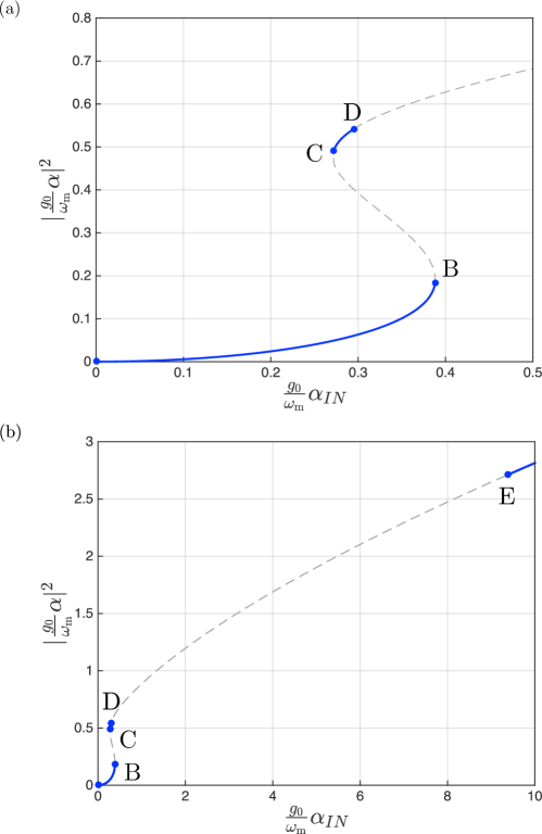
Figure 2: Optical bistability in the RP only case. The unstable branch $\mathbf{B}-\mathbf{C}$ corresponds to the lower branch, associated with the optical bistability picture (condition (16)). The unstable branch $\mathbf{D}-\mathbf{E}$ corresponds to the violation of condition (17). Plot parameters: $\Delta_{0}=-\omega_{\rm m}$, $g_{0}=10^{-5}\omega_{\rm m}$, $\kappa=0.6\omega_{\rm m}$, $\gamma=0.12\omega_{\rm m}$

The violation of the condition $a_{0}>0$ corresponds to the branch $\mathbf{B}-\mathbf{C}$ . As outlined in Aldana et al. (2013), in the pure RP case, up to linear order in $\gamma/\omega_{\rm m}$, the critical values for $|\alpha|^{2}$, corresponding to the points $B$ and $C$ (see Fig. 2) are given by

$$\left|\alpha_{B,C}\right|^{2}=-\frac{\Delta_{0}}{3\omega_{\rm m}}\left[1\pm\frac{1}{2}\sqrt{1-\frac{3\kappa^{2}}{4\Delta_{0}^{2}}}\right],$$ (18)

indexes $B$ and $C$ correspond to the lower and upper sign respectively. In presence of CK coupling, the stability picture is modified. For small values of $g_{\rm ck}$, the presence of a CK coupling increases the range of values of $|\alpha|^{2}$ for which the branch $\mathbf{B}-\mathbf{C}$ is unstable. In the resolved-sideband regime ($\kappa\ll\omega_{\rm m}=|\Delta_{0}|$) the CK result is obtained as a (first-order) expansion in $g_{\rm ck}$ from the pure RP solution

$$|\alpha^{\rm ck}_{B}|^{2}=-\frac{\Delta_{0}}{6\omega_{\rm m}}-\frac{\kappa^{2}}{16\Delta_{0}\omega_{\rm m}}-\frac{g_{\rm ck}\Delta_{0}}{4\omega_{\rm m}^{4}}\left(\Delta_{0}^{2}+\frac{3\kappa^{2}}{4}\right)$$ (19)

$$|\alpha^{\rm ck}_{C}|^{2}=-\frac{\Delta_{0}}{2\omega_{\rm m}}+\frac{\kappa^{2}}{16\Delta_{0}\omega_{\rm m}}-\frac{g_{\rm ck}\Delta_{0}}{4\omega_{\rm m}^{4}}\left(\Delta_{0}^{2}-\frac{\kappa^{2}}{4}\right).$$ (20)

However, increasing $g_{\rm ck}$ further, leads to a reduction and, eventually, the disappearance of the unstable branch $\mathbf{B}-\mathbf{C}$ (see Figs. 3 and 4).

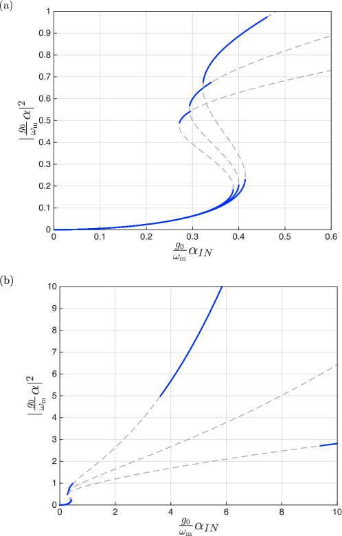
Figure 3: Effect of $g_{\rm ck}$ on the stability diagram as a function of the input drive, weak $g_{\rm ck}$. (a) The presence of the CK term reduces the input drive range for the branch $\mathbf{B}-\mathbf{C}$ (increasing $g_{\rm ck}$ for the different curves from left to right). (b) The CK term first induces a broadening of the upper unstable region, which, upon further increase, is reduced (increasing $g_{\rm ck}$ for the different curves from bottom to top). Plots parameters, $g_{\rm ck}/g_{0}^{2}=0,0.2,0.4$; other parameters same as in Fig. 2

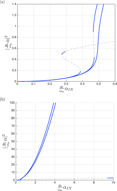
Figure 4: Effect of $g_{\rm ck}$ on the stability diagram as a function of the input drive, strong $g_{\rm ck}$. (a) The presence of the CK term reduces the input drive range for the branch $\mathbf{B}-\mathbf{C}$ (increasing $g_{\rm ck}$ for the different curves from left to right). (b) The CK term first induces a broadening of the upper unstable region, which, upon further increase, is reduced (increasing $g_{\rm ck}$ for the different curves from bottom to top). Plots parameters, $g_{\rm ck}/g_{0}^{2}=0,0.95,1$ other parameters same as in Fig. 2

In the regime for which $g_{\rm ck}|\alpha|^{2}\gg 1$, the critical value $g^{\rm c}_{\rm ck}$ for which the unstable branch $\mathbf{B}-\mathbf{C}$ disappears can be approximated by

$$g^{\rm c1}_{\rm ck}=\frac{8\omega_{\rm m}^{2}}{\kappa}\sqrt{16-\frac{\gamma^{2}}{4\omega_{\rm m}^{2}}}$$ (21)

V Stability analysis - upper branch

The condition given by Eq. (16), derived from the condition $a_{3}a_{2}a_{1}-(a_{1}^{2}+a_{3}^{2}a_{0})>0$, corresponds to the unstable branch $\mathbf{D}-\mathbf{E}$. For the pure RP case, the endpoints of the $\mathbf{D}-\mathbf{E}$ branch are (up to linear order in $\gamma/\kappa$ and $\Delta_{0}=-\omega_{\rm m}$)

$$\left|\alpha_{D}\right|^{2}=g_{0}^{-2}\left(\frac{1}{2}+\frac{\epsilon}{8}\right)$$ (22)

$$\left|\alpha_{E}\right|^{2}=g_{0}^{-2}\left(\sqrt{\frac{1}{2\epsilon}}+\frac{3}{4}+\frac{19}{32}\sqrt{2\epsilon}-\frac{\epsilon}{16}\right).$$ (23)

(where $\epsilon=\gamma/\kappa$) Analogously to the approach employed to evaluate the effect of the CK term on the $\mathbf{B}-\mathbf{C}$ branch in the small $g_{\rm ck}$ limit, we consider the perturbative correction to the RP result induced by $g_{\rm ck}$. Up to linear order, the boundaries of the unstable region $\mathbf{D}-\mathbf{E}$, for small values of $g_{\rm ck}$ ( again for $\gamma/k\ll 1$) are given by

$$\left|\alpha^{\rm ck}_{\rm D}\right|^{2}=\frac{(1+\eta_{\rm D})^{2}}{2g_{0}^{2}(1+3\eta_{\rm D}+\eta_{\rm D}^{2})}$$ (24)

$$\left|\alpha^{\rm ck}_{\rm E}\right|^{2}=\frac{3(1+\eta_{\rm E})^{2}}{32g_{0}^{2}\Lambda_{\rm E}(1+2\eta_{\rm E})^{2}}\left(\sqrt{\frac{3\kappa}{\gamma\Lambda_{\rm E}}}+3\right)$$ (25)

with

$$\Lambda_{\rm D,E}=\frac{3(1+\eta_{\rm D,E})(1+2\eta_{\rm D,E})-\eta_{\rm D,E}^{2}}{8(1+\eta_{\rm D,E})(1+2\eta_{\rm D,E})^{2}}$$

$$\eta_{\rm D,E}=\frac{g_{\rm ck}}{g_{0}^{2}}|\alpha_{\rm D,E}|^{2}.$$

Within the validity limit of the perturbative approximation, the unstable region $\mathbf{D}-\mathbf{E}$ is extended by the presence of the CK nonlinearity. Our numerical analysis shows that the region $\mathbf{D}-\mathbf{E}$ increases with increasing $g_{\rm ck}$ until a critical value $g_{\rm ck}^{*}$, for which $\mathbf{E}\to\infty$, implying that, for $g_{\rm ck}=g_{\rm ck}^{*}$, the upper branch is unstable for every $\left|\alpha\right|>\left|\alpha_{\rm D}\right|$. The value of $g_{\rm ck}^{*}$ can be evaluated considering, in the limit $|\alpha|^{2}\gg 1$, the condition given by Eq. (17) is expressed by a fourth-order polynomial in $\left|\alpha\right|^{2}$, $Q(\left|\alpha\right|^{2})$. Furthermore, the asymptotic behaviour of $Q(\left|\alpha\right|^{2})$ can be deduced from the sign of the highest-power coefficients $c_{3}^{\infty}$ and $c_{4}^{\infty}$. In this limit, we have

$$c^{\infty}_{3}=-\frac{32}{\omega_{\rm m}}\left[\frac{\gamma\kappa\Delta_{0}}{\omega_{\rm m}^{2}}+\frac{g_{\rm ck}}{g_{0}^{2}}\left\{\frac{g_{\rm ck}\gamma\kappa\Delta_{0}}{4g_{0}^{2}}+\left(\gamma+\kappa\right)\right\}\right]$$ (26)

$$c^{\infty}_{4}=\gamma\kappa\left(\frac{g_{\rm ck}^{2}}{g_{0}^{4}}-\frac{4}{\omega_{\rm m}^{2}}\right)^{2}$$ (27)

If we assume $2\Delta_{0}>g_{\rm ck}$, it is possible to see how $c^{\infty}_{3}<0$ for every value of the cavity field, while $c^{\infty}_{4}>0$, except when $g_{\rm ck}=2g_{0}^{2}/\omega_{\rm m}$. In this case $\left|\alpha_{\rm E}\right|^{2}\to\infty$, and the system remains unstable for every value of the cavity field above $\left|\alpha_{\rm D}\right|$. If $g_{\rm ck}$ is further increased above $g_{\rm ck}^{*}=2g_{0}/\omega_{\rm m}$ the region $\mathbf{D}-\mathbf{E}$ becomes finite again and eventually disappears for $g_{\rm ck}^{\rm c2}$. In the limit $\gamma/\kappa\ll 1$,

$$g_{\rm ck}^{\rm c2}\simeq-\frac{2(\gamma+\kappa)^{2}}{\gamma\kappa\Delta_{0}}g_{0}^{2}\simeq\left.2g_{\rm ck}^{*}+\frac{2\kappa g_{0}^{2}}{\omega_{\rm m}\gamma}\right|_{\Delta_{0}=-\omega_{\rm m}}.$$ (28)

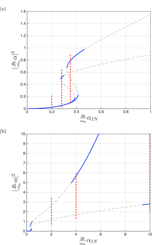
Figure 5: Same as in Fig. 3, for the puer RP case ($g_{\rm ck}=0$), and for $g_{\rm ck}=0.2$. The vertical dashed lines correspond to the input drive values for which the $\Delta_{0}$-dependence is depicted in Figs. 6-8.

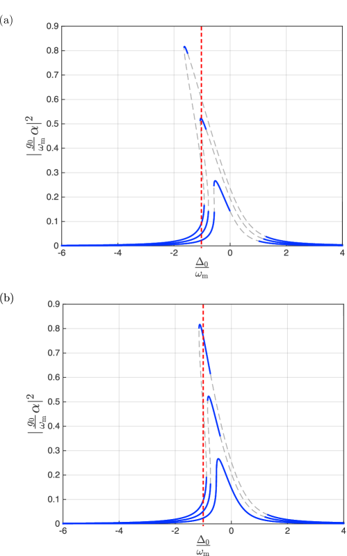
Figure 6: $\Delta_{0}$ dependence of the cavity population in (a) the pure RP case and (b) in the CK ($g_{\rm ck}=0.2$) case. Increasing $\alpha_{\rm IN}=0.2,0.28,0.35$ in units of $\omega_{\rm m}/g_{0}$ for increasing peak height. The presence of the CK term leads to a larger parameter range for which stability is observed.

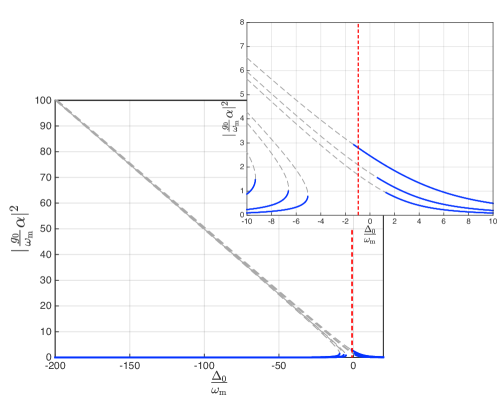
Figure 7: $\Delta_{0}$ dependence of the cavity population in the pure RP case. Increasing $\alpha_{\rm IN}=2,4,10$ in units of $\omega/g_{0}$ for increasing peak height (see inset). The case $\alpha_{\rm IN}=10\omega/g_{0}$ outlines the mechanism thorough which the result for $\Delta_{0}=-\omega$ is stable at large drives (vertical dashed line).

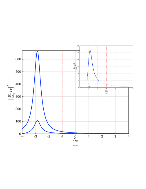
Figure 8: $\Delta_{0}$ dependence of the cavity population in the CK ($g_{\rm ck}=0.2$) case. Increasing $\alpha_{\rm IN}=$ ($2,4,10\omega/g_{0}$) for increasing peak height. It is possible to see how, for large values of the input field, the system is stable for every value of detuning $\Delta_{0}$. The case $\alpha_{\rm IN}=2\omega/g_{0}$ outlines the peculiar (“reentrant”) peak shape for intermediate input drive.

VI Conclusion

In this paper, we have shown how the addition of an additional cross-Kerr coupling term to the usual radiation-pressure coupling term in the description of the dynamics of optomechanical systems substantially modifies the stability properties of the corresponding semiclassical equations of motion. In particular, we have shown how the inclusion of a CK term leads to an alteration and, eventually, to the disappearance of the unstable branch $\mathbf{B}-\mathbf{C}$, for $g_{\rm ck}>g^{\rm c1}_{\rm ck}$. Analogously, the unstable branch $\mathbf{D}-\mathbf{E}$ is affected by the presence of a CK coupling term: for values of $g_{\rm ck}\in\left]0,g^{*}_{\rm ck}\right]$ the branch $\mathbf{D}-\mathbf{E}$ is extended ($\mathbf{E}\to\infty$, for $g_{\rm ck}=g_{\rm ck}^{*}$ ), while, upon further increase of $g_{\rm ck}$, the branch $\mathbf{D}-\mathbf{E}$ shrinks and, eventually, disappears for $g_{\rm ck}=g_{\rm ck}^{\rm c2}$

cross-Kerr coupling constant $g_{\rm ck}$ is increased.

VII Acknowledgements

This work was supported by the Academy of Finland (project “Quantum properties of optomechanical systems”).

References

- Aspelmeyer et al. (2014) M. Aspelmeyer, T. J. Kippenberg, and F. Marquardt, Rev. Mod. Phys. 86, 1391 (2014).
- Ano (2015a) “The VIRGO interferometer,” (2015a).
- Ano (2015b) “LSC - LIGO Scientific Collaboration,” (2015b).
- Teufel et al. (2011) J. D. Teufel, T. Donner, D. Li, J. W. Harlow, M. S. Allman, K. Cicak, A. J. Sirois, J. D. Whittaker, K. W. Lehnert, and R. W. Simmonds, Nature 475, 359 (2011).
- Andrews et al. (2014) R. W. Andrews, R. W. Peterson, T. P. Purdy, K. Cicak, R. W. Simmonds, C. A. Regal, and K. W. Lehnert, Nat. Phys. 10, 321 (2014).
- Massel et al. (2011) F. Massel, T. T. Heikkilä, J. M. Pirkkalainen, S. U. Cho, H. Saloniemi, P. J. Hakonen, and M. A. Sillanpää, Nature 480, 351 (2011).
- Rabl (2011) P. Rabl, Phys. Rev. Lett. 107, 063601 (2011).
- Nunnenkamp et al. (2011) A. Nunnenkamp, K. Børkje, and S. Girvin, Phys. Rev. Lett. 107, 063602 (2011).
- Heikkilä et al. (2014) T. T. Heikkilä, F. Massel, J. Tuorila, R. Khan, and M. A. Sillanpää, Phys. Rev. Lett. 112, 203603 (2014).
- Pirkkalainen et al. (2015) J. M. Pirkkalainen, S. U. Cho, F. Massel, J. Tuorila, T. T. Heikkilä, P. J. Hakonen, and M. A. Sillanpää, Nat Commun 6, 6981 (2015).
- Seok et al. (2013) H. Seok, L. F. Buchmann, E. M. Wright, and P. Meystre, Phys. Rev. A 88, 063850 (2013).
- Jayich et al. (2008) A. M. Jayich, J. C. Sankey, B. M. Zwickl, C. Yang, J. D. Thompson, S. M. Girvin, A. A. Clerk, F. Marquardt, and J. G. E. Harris, New J Phys 10, 095008 (2008).
- Purdy et al. (2010) T. Purdy, D. Brooks, T. Botter, N. Brahms, Z. Y. Ma, and D. Stamper-Kurn, Phys. Rev. Lett. 105, 133602 (2010).
- Xuereb and Paternostro (2013) A. Xuereb and M. Paternostro, PRA 87, 023830 (2013).
- Nemoto and Munro (2004) K. Nemoto and W. J. Munro, Phys. Rev. Lett. 93, 250502 (2004).
- Sheng et al. (2012) Y.-B. Sheng, L. Zhou, S.-M. Zhao, and B.-Y. Zheng, Phys. Rev. A 85, 012307 (2012).
- Sheng and Zhou (2015) Y.-B. Sheng and L. Zhou, Sci. Rep. 5, 7815 (2015).
- Sheng et al. (2010) Y.-B. Sheng, F.-G. Deng, and G. L. Long, Phys. Rev. A 82, 032318 (2010).
- Walls and Milburn (2007) D. F. Walls and G. J. Milburn, Quantum Optics (Springer, Berlin, 2007).
- Aldana et al. (2013) S. Aldana, C. Bruder, and A. Nunnenkamp, Phys. Rev. A 88, 043826 (2013).
- Marquardt et al. (2007) F. Marquardt, J. P. Chen, A. A. Clerk, and S. M. Girvin, Phys. Rev. Lett. 99, 093902 (2007).
- Khan et al. (2015) R. Khan, F. Massel, and T. T. Heikkilä, Phys. Rev. A 91, 043822 (2015).