Tunneling dynamics of two interacting one-dimensional particles

Abstract

We present one-dimensional simulation results for the cold atom tunneling experiments by the Heidelberg group [G. Zürn et al., Phys. Rev. Lett. 108, 075303 (2012) and G. Zürn et al., Phys. Rev. Lett. 111, 175302 (2013)] on one or two ⁶Li atoms confined by a potential that consists of an approximately harmonic optical trap plus a linear magnetic field gradient. At the non-interacting particle level, we find that the WKB (Wentzel-Kramers-Brillouin) approximation may not be used as a reliable tool to extract the trapping potential parameters from the experimentally measured tunneling data. We use our numerical calculations along with the experimental tunneling rates for the non-interacting system to reparameterize the trapping potential. The reparameterized trapping potentials serve as input for our simulations of two interacting particles. For two interacting (distinguishable) atoms on the upper branch, we reproduce the experimentally measured tunneling rates, which vary over several orders of magnitude, fairly well. For infinitely strong interaction strength, we compare the time dynamics with that of two identical fermions and discuss the implications of fermionization on the dynamics. For two attractively-interacting atoms on the molecular branch, we find that single-particle tunneling dominates for weakly-attractive interactions while pair tunneling dominates for strongly-attractive interactions. Our first set of calculations yields qualitative but not quantitative agreement with the experimentally measured tunneling rates. We obtain quantitative agreement with the experimentally measured tunneling rates if we allow for a weakened radial confinement.

I Introduction

Open quantum systems are at the heart of many physical phenomena from nuclear physics to quantum information theory Breuer and Petruccione (2007); Wiseman and Milburn (2010). In fact, all “real” quantum systems are, to some extent, open systems. Interactions with the environment cause decoherence, resulting in non-equilibrium dynamics. It is often simpler to design experiments that probe non-equilibrium physics than it is to design experiments that probe equilibrium physics. Conversely, the theoretical toolkit for describing systems in equilibrium is generally much farther developed than that for describing systems in non-equilibrium.

Ultracold atom systems provide a platform for realizing clean and tunable quantum systems Bloch et al. (2008); Blume (2012); Giorgini et al. (2008); Chin et al. (2010). Over the past few years, much effort has gone into describing non-equilibrium experiments that are accessible, within approximate or exact frameworks, to theory. Notable experiments are the equilibration dynamics of one-dimensional Bose gases Langen et al. (2015), the spin dynamics of dipolar molecules in optical lattices with low filling factor Yan et al. (2013), and the tunneling dynamics of effectively one-dimensional few-fermion systems Zürn et al. (2012, 2013a). This paper focuses on the latter set of experiments. Specifically, the goal of the present work is to describe the tunneling dynamics of few-fermion systems, which are prepared in a well defined quasi-eigenstate (metastable state), into free space. We consider small systems and directly solve the time-dependent Schrödinger equation in coordinate space. As we will show, this approach provides a means to quantify the importance of the particle-particle interaction, covering time scales from a fraction of the trap scale to thousands times the trap scale. Alternatively, one could adopt a quantum optics perspective and pursue a master equation approach.

Tunneling is arguably the most quantum phenomenon there is: If the system was behaving classically, tunneling would be absent Razavy (2013). Tunneling plays an important role across physics, chemistry and technology. The scanning tunneling microscope Oka et al. (2014), for example, nicely illustrates how a physics phenomenon, the tunneling of electrons, has been turned into a powerful practical tool (the imaging of materials). The $\alpha$-decay, i.e., the decay of a ⁴He nucleus from a heavy nucleus, is an example discussed in most undergraduate physics texts (see, for example, Ref. Serway et al. (2004)). The typical picture is to identify an effective reaction coordinate and to obtain the tunneling rate from a WKB analysis. While powerful, such treatments completely neglect the effect of interactions. Interactions also play a crucial role in sorting out under which conditions electrons in light atoms tunnel sequentially or simultaneously Eckle et al. (2008). The two-particle system considered in this work has been realized experimentally and is the possibly simplest scenario that deals with a truly open quantum system (the atoms can escape to infinity) in which interactions (short-range atom-atom interactions) play a crucial role. As we will show, even for this relatively simple set-up, matching theory and experiment is a non-trivial task. Of course, two-particle tunneling has been investigated previously in this and related contexts Lode et al. (2012); Hunn et al. (2013); Kim and Brand (2011); Lode et al. (2009); Rontani (2012, 2013); Lundmark et al. (2015).

The remainder of this paper is organized as follows. Section II introduces the Hamiltonian, the Heidelberg experiment and selected simulation details. Sections III and IV discuss the molecular and upper branch tunneling dynamics. For both cases, it is argued that the trapping potential needs to be reparameterized. Using the reparameterized trapping potential, numerical simulations for the tunneling dynamics of two distinguishable ⁶Li atoms on the molecular branch and the upper branch are discussed. Comparisons with the experimentally measured tunneling rates are presented. Finally, Sec. V summarizes and provides an outlook. Simulation details and some technical aspects are relegated to Appendices A–G.

II System Hamiltonian and simulation details

II.1 One-body Hamiltonian, WKB analysis, and Heidelberg experiment

This section considers a single ⁶Li atom with mass $m$. The atom is assumed to be in the hyperfine state $|F,m_{F}\rangle$. We consider the three lowest hyperfine states of the ⁶Li atom, referred to as $|1\rangle=|1/2,1/2\rangle$, $|2\rangle=|1/2,-1/2\rangle$, and $|3\rangle=|3/2,-3/2\rangle$. Figure 1

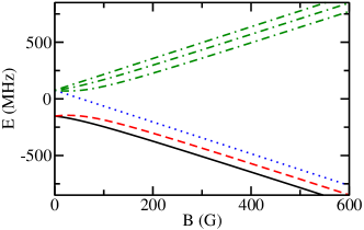
Figure 1: (Color online) Energy of the hyperfine states of ⁶Li as a function of the magnetic field strength $B$. Solid, dashed and dotted lines correspond to states $|1\rangle$, $|2\rangle$, and $|3\rangle$, respectively (see text for details). States $|1\rangle$ and $|2\rangle$ are used in the upper branch experiments Zürn et al. (2012), while states $|1\rangle$ and $|3\rangle$ are used in the molecular branch experiments Zürn et al. (2013a). The higher-lying energy states shown by dash-dotted lines are not relevant for the present paper.

shows the dependence of the hyperfine energy levels on the magnetic field strength $B$. The atom with coordinates $(x,y,z)$ is trapped optically in a non-separable potential that is much tighter in the $\rho$-direction ($\rho^{2}=x^{2}+y^{2}$) than in the $z$-direction Zürn et al. (2012, 2013a). Throughout this work, we do not simulate the motion in the tight transverse confining direction. The transverse trapping frequency does, however, enter into the calculation of the renormalized one-dimensional coupling constant (see Sec. II.3). Evaluating the confinement created by the gaussian laser beam at $\rho=0$, the effective one-dimensional single-particle Hamiltonian $H^{\text{sp}}$ reads Zürn et al. (2012, 2013a)

$$H^{\text{sp}}(z,t;p,z_{\text{R}},\mathcal{C}_{|j\rangle}(B))=-\frac{\hbar^{2}}{2m}\frac{\partial^{2}}{\partial z^{2}}$$

$$+V_{\text{trap}}(z,t;p,z_{\text{R}},\mathcal{C}_{|j\rangle}(B)),$$ (1)

where the trapping potential $V_{\text{trap}}$ along the $z$-direction depends implicitly on the internal or hyperfine state $|j\rangle$ of the atom through the coefficient $\mathcal{C}_{|j\rangle}$,

$$V_{\text{trap}}(z,t;p,z_{\text{R}},\mathcal{C}_{|j\rangle}(B))=$$

$$p(t)V_{0}\left(1-\frac{1}{\left(z/z_{\text{R}}\right)^{2}+1}\right)-\mu_{\text{B}}\mathcal{C}_{|j\rangle}(B)z.$$ (2)

The first term on the right hand side of Eq. (2) accounts for the optical confinement. $V_{0}$ denotes the maximum depth of the trap, $p(t)$ a time-dependent parameter [$p(t)\leq 1$], and $z_{\text{R}}$ the Rayleigh range of the laser beam that produces the confinement. The second term on the right hand side of Eq. (2) is linear in $z$ and makes the tunneling possible. $\mu_{\text{B}}$ is the Bohr magneton and $\mathcal{C}_{|j\rangle}(B)$ depends on the hyperfine state, magnetic field strength and magnetic field gradient $B^{\prime}$,

$$\mathcal{C}_{|j\rangle}(B)=c_{|j\rangle}(B)B^{\prime}.$$ (3)

Here, $c_{|j\rangle}(B)$ is a dimensionless parameter close to $1$ (see below for details). Table 1

Table 1: Parameters from Refs. Zürn et al. (2012, 2013a) that define the trapping potential. Since the energy of the two-particle system on the molecular branch is smaller than the energy of the two-particle system on the upper branch, the $p(t=0)$ value for the molecular branch is chosen to be smaller than that for the upper branch; this guarantees that the tunneling rates for the two experiments have roughly comparable orders of magnitude. The harmonic oscillator units are defined in terms of $\omega=2\pi\times 1234$Hz, corresponding to $E_{\text{ho}}=8.177\times 10^{-31}$J, $a_{\text{ho}}=1.167\mu$m, and $\omega^{-1}=1.290\times 10^{-4}$s, or $1\text{J}=1.223\times 10^{30}E_{\text{ho}}$, $1\text{m}=8.570\times 10^{5}a_{\text{ho}}$, and $1\text{s}=7753\omega^{-1}$. In an alternative levitation measurement, the magnetic field gradient was found to be $B^{\prime}=1890(20)$G/m Zürn et al. (2012).

Quantity	Value
$V_{0}$	$k_{B}\times 3.326\mu\text{K}=56.16E_{\text{ho}}$
$z_{\text{R}}$	$9.975(5)\times 10^{-6}\text{m}=8.548(5)a_{\text{ho}}$
$p(-t_{r})$	$0.795$
$p(t=0)$ (upper branch)	$0.6875$
$p(t=0)$ (molecular branch)	$0.63496$
$dp/dt$ (for $-t_{r}<t<0$)	$-43\text{s}^{-1}$
$B^{\prime}$ (WKB approximation)	$1892$G/m

summarizes the trap parameters reported by the Heidelberg group Zürn et al. (2012, 2013a); the parameters are obtained from a combination of measurement and WKB analysis. Figure 2

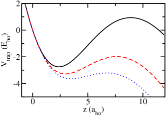
Figure 2: (Color online) The trapping potential, Eq. (2), for $\mathcal{C}=1892$G/m and three different values of $p$, $p=0.795$ (solid line), $p=0.6875$ (dashed line), and $p=0.63496$ (dotted line). $V_{0}$ and $z_{\text{R}}$ are fixed at the values reported in Table 1.

shows $V_{\text{trap}}$ for $\mathcal{C}=1892$G/m and three different values of $p$. The solid line shows the typical confinement at the beginning of the experiment while the dashed and dotted lines show typical confinements during the hold time of the upper branch and molecular branch experiments, respectively (see below for details).

Since the trapping potential changes with time, there exists no set of units that characterizes the system equally well for all times. Throughout, following Ref. Zürn et al. (2012), we choose $\omega=2\pi\times 1234$Hz to define the oscillator units $E_{\text{ho}}$, $a_{\text{ho}}$, and $T_{\text{ho}}$: $E_{\text{ho}}=\hbar\omega$, $a_{\text{ho}}=\sqrt{\hbar/(m\omega)}$, and $T_{\text{ho}}=2\pi/\omega$.

The confining potential $V_{\text{trap}}$ has a local minimum at $z_{\text{min}}$ and a local maximum at $z_{b}$. To gain insight into the harmonic approximation, we expand $V_{\text{trap}}$ around its local minimum and calculate the frequency $\omega_{\text{trap}}(p)$ of the harmonic term,

$$\omega_{\text{trap}}(p)=\sqrt{2\frac{p(t)V_{0}}{m}\frac{\left(z_{\text{R}}^{4}-3z_{\text{R}}^{2}z_{\text{min}}^{2}\right)}{\left(z_{\text{R}}^{2}+z_{\text{min}}^{2}\right)^{3}}}.$$ (4)

In the absence of the magnetic field gradient $B^{\prime}$, the minimum of $V_{\text{trap}}$ is located at $z_{\text{min}}=0$. For a finite magnetic field gradient, the local minimum $z_{\text{min}}$ depends on the parameters of the trapping potential. The frequency $\omega_{\text{trap}}(p)$ can differ notably from the frequency $\omega$ and provides, in some cases, a more natural unit. We define $E_{\text{trap}}(p)=\hbar\omega_{\text{trap}}(p)$, $a_{\text{trap}}(p)=\sqrt{\hbar/(m\omega_{\text{trap}}(p))}$, and $T_{\text{trap}}(p)=2\pi/\omega_{\text{trap}}(p)$. Note that these units depend explicitly on $p(t)$; correspondingly, we specify $p(t)$ when we use these units.

The single-particle tunneling dynamics is, to a good approximation, described by an exponential decay,

$$P_{\text{sp,in}}(t)=P_{\text{sp,in}}(t_{\text{ref}})\exp[-\gamma_{\text{sp}}(t-t_{\text{ref}})],$$ (5)

where $P_{\text{sp,in}}(t)$ denotes the probability of finding the particle inside the trap, the tunneling rate $\gamma_{\text{sp}}$ is assumed to be constant, and $t_{\text{ref}}$ is a reference time. Within the WKB approximation (see, e.g., Ref. Ankerhold (2007)), the tunneling rate $\gamma_{\text{sp}}^{\text{WKB}}$ reads

$$\gamma_{\text{sp}}^{\text{WKB}}=f^{\text{WKB}}{\mathcal{T}},$$ (6)

where the frequency $f^{\text{WKB}}$ and the tunneling coefficient ${\mathcal{T}}$ are given by

$$f^{\text{WKB}}=\frac{\epsilon-V_{\text{trap}}(z_{\text{min},t=0})}{2\pi\hbar}$$ (7)

and

$${\mathcal{T}}=\exp\left(-2\int_{z_{\epsilon,2}}^{z_{\epsilon,3}}\sqrt{\frac{2m}{\hbar^{2}}|\epsilon-V_{\text{trap}}(z)|}dz\right).$$ (8)

In Eqs. (7)-(8), $V_{\text{trap}}$ is the trapping potential with $p(t=0)$ (see Fig. 3 for the time dependence of $p$), $z_{\text{min},t=0}$ is the $z$-value at which $V_{\text{trap}}$ with $p(t=0)$ takes its local minimum, and the WKB energy $\epsilon$ of state $n$ is found by the consistency condition

$$\int_{z_{\epsilon,1}}^{z_{\epsilon,2}}\sqrt{2m[\epsilon-V_{\text{trap}}(z)]}dz=\left(n+\frac{1}{2}\right)\pi\hbar.$$ (9)

Here, $z_{\epsilon,1}$, $z_{\epsilon,2}$, and $z_{\epsilon,3}$ with $z_{\epsilon,1}<z_{\epsilon,2}<z_{\epsilon,3}$ are the three solutions of $\epsilon-V_{\text{trap}}(z)=0$ and $n$ with $n=0,1,2,\dots$ denotes the order of the semiclassical “bound state” of the trap. In theory, one has $P_{\text{sp,in}}(t)+P_{\text{sp,out}}(t)=1$, with the initial condition $P_{\text{sp,in}}(-t_{r})=1$. Here $P_{\text{sp,out}}(t)$ denotes the probability that the particle has left the trap. The inside and outside regions are defined through $z<z_{b}$ and $z>z_{b}$, respectively, with $z_{b}$ corresponding to the barrier position at time $t=-t_{r}$.

We now briefly review the experimental sequence employed by the Heidelberg group Zürn et al. (2012, 2013a). The experiment prepared the atom in an “eigenstate” of the deep trap ($p=0.795$ at $t=-t_{r}$) and then lowered the barrier by decreasing $p(t)$ over a time period $t_{r}$. At time $t=0$, $p(t)$ reached its minimum. After a variable hold time $t_{\text{hold}}$, the barrier was ramped back up over a time period $t_{r}$. At time $t=t_{\text{hold}}+t_{r}$, the experiment monitored the fraction $P_{\text{sp,out}}(t)$ of the particle that had left the trap. To obtain $P_{\text{sp,out}}(t)$, the experiment was repeated many times for each $t=t_{\text{hold}}+t_{r}$ and the data were averaged [each individual experiment yields $P_{\text{sp,out}}(t_{\text{hold}}+t_{r})=0$ or 1]. The time sequence is sketched in Fig. 3.

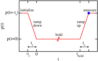
Figure 3: (Color online) Schematic of the time sequence of the experiment. After initialization of the system, the dimensionless parameter $p(t)$ decreases from $p(t=-t_{r})$ to $p(t=0)$ with a rate $dp/dt=-43$ s^-1, remains constant for $t_{\text{hold}}$ ($t_{\text{hold}}\gg t_{r}$), and increases to its initial value over the time period $t_{r}$. The measurement is performed at the time $t_{\text{hold}}+t_{r}$.

In the experiment Zürn et al. (2013a), the initial condition was $P_{\text{sp,in}}(-t_{r})<1$ due to non-unit state preparation fidelity. While this changes the overall normalization, it does not change the tunneling dynamics.

The coefficients $c_{|j\rangle}(B)$, and correspondingly the $\mathcal{C}_{|j\rangle}(B)$, depend on the magnetic field strength $B$, which is used to tune the atom-atom scattering length. The coefficients $c_{|j\rangle}(B)$ can, at least in a first analysis, be obtained using the Breit-Rabi formula Breit and Rabi (1931) (see Appendix A). For state $|3\rangle$, the Breit-Rabi coefficient $c_{|3\rangle}^{\text{BR}}(B)$ is independent of the magnetic field. For states $|1\rangle$ and $|2\rangle$, the dependence of the Breit-Rabi coefficients on the magnetic field strength $B$ is comparatively strong when $B$ is small ($B\lesssim 600$G) and weak when $B\to\infty$ ($B\gtrsim 600$G). References Zürn et al. (2012, 2013a) did not use the Breit-Rabi formula to determine the $c_{|j\rangle}(B)$ coefficients (see below for details).

To parameterize $V_{\text{trap}}$, Refs. Zürn et al. (2012, 2013a) fed the result from “calibration measurements” into Eqs. (6) and (9). In a first step, the parameters $V_{0}$ and $z_{\text{R}}$ of the optical trap, which is independent of the hyperfine state and magnetic field strength, were calibrated assuming $p=1$. Specifically, the single-particle trap energy levels of the pure optical trap [${\mathcal{C}}_{|j\rangle}(B)=0$ in Eq. (2)] were measured spectroscopically and the parameters $V_{0}$ and $z_{\text{R}}$ were chosen such that the WKB energy levels agreed with the measured energies (see the supplemental material of Ref. Zürn et al. (2012)).

For the upper branch tunneling experiment, $p(t=-t_{r})$ and $p(t=0)$ were obtained by measuring the relative integrated light intensities of the trap beams, i.e., $p(t=-t_{r})$ and $p(t=0)$ were calibrated relative to $p=1$ Zur (May 7, 2015). To obtain $B^{\prime}$, tunneling experiments at various magnetic fields using ⁶Li in state $|2\rangle$ were performed footnote7a . To prepare the atom in an excited trap state, the experiments used a trick. Two atoms in the same hyperfine states were prepared in the trap (these atoms do not interact), forcing the two-particle system to sit in a superposition of the lowest and first excited trap states. The assumption was then that the tunneling dynamics proceeds as if there were a single particle in the first excited trap state and another single particle in the lowest trap state. The tunneling was attributed to the particle in the first excited trap state while the particle in the lowest trap state was assumed to have no chance of tunneling. This assumption is, as our simulations show, justified quite well (see Appendix B). To analyze the tunneling data, $c_{|j\rangle}$ was assumed to be equal to 1 for all magnetic field strengths and $B^{\prime}$ was adjusted to yield a WKB tunneling rate $\gamma_{\text{sp}}^{\text{WKB}}$ that agreed with the measured tunneling rate $\gamma_{\text{sp}}^{\text{exp}}$. The resulting $B^{\prime}$ was then used for all hyperfine states.

The two-particle molecular branch experiments were conducted at magnetic field strengths varying from $350$G to $1202$G and utilized states $|1\rangle$ and $|3\rangle$ Zürn et al. (2013a). The parameters $p(t=-t_{r})$, $V_{0}$, $z_{\text{R}}$, and $B^{\prime}$ were taken as those obtained from the upper branch experiments. Compared to the upper branch experiments, $p(t=0)$ was reduced to obtain tunneling times smaller than a few thousand milliseconds and the magnetic field dependence of the coefficients $c_{|j\rangle}(B)$ was found to play a non-negligible role. For technical reasons, $p(t=0)$ was not calibrated via a “direct” photodetector measurement Zur (May 7, 2015). Instead, $p(t=0)$ and $c_{|j\rangle}(B)$ were determined based on the WKB analysis of the experimentally measured single-particle tunneling rates (see supplemental material of Ref. Zürn et al. (2013a)). Specifically, the single-particle tunneling measurements were performed at $B=350$G and $569$G and the parameters $p(t=0)$ and $c_{|j\rangle}(B)$ were adjusted to yield a WKB value $\gamma_{\text{sp}}^{\text{WKB}}$ that agreed with the measured tunneling rate $\gamma_{\text{sp}}^{\text{exp}}$ at both $B$-fields (see supplemental material of Ref. Zürn et al. (2013a)). The analysis yielded $p(t=0)=0.63496$ Zürn et al. (2013a). The $c_{|1\rangle}(B)$ and $c_{|3\rangle}(B)$ values are given in Table 2.

II.2 Simulation of single-particle tunneling dynamics

To determine the single-particle tunneling rate theoretically, we prepare the initial state ($t\leq-t_{r}$) through imaginary time propagation. The initial state can be thought of as a quasi-eigenstate. We then propagate the initial state in real time for $t>-t_{r}$. For $-t_{r}<t<0$, we change $p(t)$ according to $dp/dt=-43\text{s}^{-1}$. For $t>0$, $p(t)$ is kept constant, i.e., $p(t)=p(0)$. By analyzing the flux through $z=z_{b}$, we calculate $P_{\text{sp,in}}(t)$ and $P_{\text{sp,out}}(t)$. We do not simulate the up ramp, i.e., the time period $t_{\text{hold}}<t<t_{\text{hold}}+t_{r}$, since we found that the populations $P_{\text{sp,in}}(t)$ and $P_{\text{sp,out}}(t)$ do not change appreciably during the up-ramp. The simulation details are described in Appendices C and D.

II.3 Two-body Hamiltonian and simulation of two-particle tunneling dynamics

This section considers two ⁶Li atoms, each described by the single-particle Hamiltonian $H^{\text{sp}}$ [see Eq. (1)], that interact through the short-range potential $V_{\text{int}}(z_{12})$, where $z_{12}=z_{1}-z_{2}$. The two-body Hamiltonian $H$ reads

$$H(z_{1},z_{2},t;p,z_{\text{R}},\mathcal{C}_{|j_{1}\rangle}(B),\mathcal{C}_{|j_{2}\rangle}(B))=$$

$$H^{\text{sp}}(z_{1},t;p,z_{\text{R}},\mathcal{C}_{|j_{1}\rangle}(B))+$$

$$H^{\text{sp}}(z_{2},t;p,z_{\text{R}},\mathcal{C}_{|j_{2}\rangle}(B))+V_{\text{int}}(z_{12}).$$ (10)

Since the range of the true ⁶Li-⁶Li van der Waals potential is, for the experiments considered, much smaller than the de Broglie wavelength of the atoms, the details of the interaction potential are not probed and the true interaction potential can be replaced by a simpler model potential that has the same three-dimensional $s$-wave scattering length $a_{\text{3D}}$ as the true atom-atom potential. For ⁶Li the most precise magnetic field dependence of $a_{\text{3D}}$ is given in Ref. Zürn et al. (2013b). To convert $a_{\text{3D}}$ to the one-dimensional coupling constant $g_{1\text{D}}$, we assume a three-dimensional zero-range potential and strictly harmonic confinement with angular frequency $\omega_{\rho}$ in the tight direction. Describing the two-body interaction potential along the $z$-direction by

$$V_{\text{ZR}}(z_{12})=g_{1\text{D}}\delta(z_{12}),$$ (11)

the renormalized one-dimensional coupling constant $g_{1{\text{D}}}$ is given by Olshanii (1998)

$$\frac{g_{1\text{D}}}{\hbar\omega_{\rho}a_{\rho}}=\frac{2a_{\text{3D}}}{a_{\rho}}\left(1-\frac{|\zeta(1/2)|}{\sqrt{2}}\frac{a_{\text{3D}}}{a_{\rho}}\right)^{-1},$$ (12)

where $\zeta(1/2)$ is equal to $-1.46035$ and $a_{\rho}$ denotes the harmonic oscillator length in the tight confining direction, $a_{\rho}=\sqrt{\hbar/(m\omega_{\rho})}$. The one-dimensional coupling constant $g_{\text{1D}}$ and the one-dimensional scattering length $a_{1\text{D}}$ are related via $a_{1\text{D}}=-2\hbar^{2}/(mg_{1\text{D}})$. To determine $\omega_{\rho}$, Ref. Sala et al. (2013) analyzed the optical single-particle trap with $p(t)=1$ in the absence of the magnetic field gradient, accounting for the longitudinal (weak) and transverse (tight) directions. The harmonic frequency $\omega_{\rho}$ in the transverse direction was found to be $\omega_{\rho}^{\text{ref}}=2\pi\times 14.22(35)$kHz Sala et al. (2013). For $p(t)\neq 1$, $\omega_{\rho}^{\text{ref}}$ needs to be multiplied by $\sqrt{p(t)}$, i.e., $\omega_{\rho}=\sqrt{p(t)}\omega_{\rho}^{\text{ref}}$ Zürn et al. (2012, 2013a); Sala et al. (2013), resulting in a time-dependent $g_{\text{1D}}$. As discussed at the beginning of Sec. III.2, the time dependence of $g_{\text{1D}}$ has a negligible affect on the tunneling rate and we neglect it for the calculations presented in Secs. III.2 and IV.2.

The addition of the linear term [second term on the right hand side of Eq. (2)] moves the atoms away from the origin to positive $z$ values. Using Eq. (3) of the supplemental material of Ref. Sala et al. (2013) to model the confinement created by the gaussian beam in the longitudinal and transverse directions and expanding around $\rho=0$, one finds that the harmonic frequency in the transverse direction decreases with increasing $z$. For $z=z_{\text{min}}$ ($z=z_{b}$), we find that the harmonic frequency in the $\rho$-direction decreases by around 14% (38%) and 11% (44%) for the molecular and upper branches, respectively, compared to the frequencies for $z=0$. This suggests that the tight confinement length $a_{\rho}$ in the presence of the magnetic field gradient may be larger than $[p(t=0)]^{-1/4}a_{\rho}^{\text{ref}}$, where $a_{\text{ref}}=\sqrt{\hbar/(m\omega_{\rho}^{\text{ref}})}$, and correspondingly that the coupling constant $g_{1\text{D}}$ is modified. We return to this aspect in Secs. III.2 and IV.2. We reemphasize that the renormalization prescription given in Eq. (12) relies on the harmonicity of the confinement. It is well documented in the literature that this renormalization prescription is modified by anharmonicities Peng et al. (2011); Peano et al. (2005); Melezhik and Schmelcher (2009).

For the molecular branch, it has been shown theoretically that the strictly one-dimensional energies for the system without tunneling agree quite well with the full three-dimensional energies provided the one-dimensional scattering length $a_{1\text{D}}$ is larger than the harmonic oscillator length $a_{\rho}$ Gharashi et al. (2014). Correspondingly, we restrict our molecular branch calculations to this regime (i.e., the smallest $a_{1\text{D}}$ considered in Sec. III.2—calculated using $\omega_{\rho}=\sqrt{p(t=0)}\omega_{\rho}^{\text{ref}}$—is $a_{1\text{D}}=1.113a_{\text{ho}}$, corresponding to $g_{1\text{D}}=-1.797a_{\text{ho}}$). It should be kept in mind, however, that the validity regime of the one-dimensional framework could be different for static (energies) and dynamic (tunneling) observables.

We use two different model interaction potentials $V_{\text{int}}$, a zero-range potential $V_{\text{ZR}}$, Eq. (11), and a finite-range gaussian potential $V_{\text{FR}}$,

$$V_{\text{FR}}(z_{12})=-V_{\text{G}}\exp\left(-\frac{z_{12}^{2}}{2z_{0}^{2}}\right),$$ (13)

where $V_{\text{G}}$ and $z_{0}$ denote the depth ($V_{\text{G}}>0$) and the range of the interaction. We use $z_{0}=0.3a_{\text{ho}},0.2a_{\text{ho}}$ and $0.1a_{\text{ho}}$, and adjust $V_{\text{G}}$ for each $z_{0}$ such that $V_{\text{FR}}$ yields the desired one-dimensional two-body coupling constant $g_{1\text{D}}$. Throughout, $V_{\text{G}}$ is chosen such that $V_{\text{FR}}$ supports at most one even parity bound state in free space. We find that the dependence of the tunneling observables on the range $z_{0}$ is small. This together with the fact that $V_{\text{ZR}}$ and $V_{\text{FR}}$ yield compatible tunneling results (as discussed below, we checked this for selected parameter combinations) justifies the use of comparatively large $z_{0}$. The real time propagation of the two-particle system is discussed in Appendices C and E.

To get a first feeling for the two-particle system, we consider the system with $p=p(-t_{r})$ and map out the energy spectrum as a function of $g_{1\text{D}}$. We use the imaginary time propagation (see Appendix D) to find the “eigenenergies” and “eigenfunctions” of the system [strictly speaking, the states are metastable due to the finite barrier for $p(-t_{r})=0.795$]. Figure 4

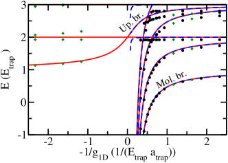
Figure 4: (Color online) Energies of two interacting trapped particles as a function of $-1/g_{1\text{D}}$. Solid and dashed lines show the energies for two particles with zero-range interaction and finite-range interaction, respectively, in a harmonic trap with frequency $\omega_{\text{trap}}$. Circles and diamonds show the energies for two particles with zero-range interaction and finite-range interaction, respectively, in an anharmonic trap [see Eq. (2)]. Both particles feel the same external potential [$p=0.795$, $c_{|j\rangle}(B)=1.00115$, and $B^{\prime}=1892$G/m, corresponding to $\omega_{\text{trap}}=2\pi\times 1067.87$Hz]. The width of the finite-range potential is $z_{0}=0.0930a_{\text{trap}}$.

shows the spectrum for two interacting particles described by the Hamiltonian $H$, Eq. (10), with $p=0.795$ and $z_{\text{R}}=8.548a_{\text{ho}}$ as a function of $-1/g_{1\text{D}}$. Both particles are assumed to feel the same single-particle trapping potential with $\mathcal{C}=1894.18$G/m. Diamonds and circles show the energies for the zero-range potential and the finite-range potential with $z_{0}=0.1a_{\text{ho}}=0.0930a_{\text{trap}}$, respectively. Note, throughout we use the zero-range potential to describe the positive $g_{1\text{D}}$ portion of the upper branch. In this regime, the Hamiltonian with finite-range interaction supports many deep-lying states, making it challenging to select the low-energy states of interest (recall, the relative and center-of-mass degrees of freedom are coupled). Alternatively, one might consider using a purely repulsive finite-range two-body potential. In this case, however, a large $g_{1\text{D}}$ would require a large range, thereby making the calculations model-dependent. Hence, this alternative approach is not pursued here. Figure 4 uses the natural units $a_{\text{trap}}$ and $E_{\text{trap}}$ with $\omega_{\text{trap}}=2\pi\times 1067.87$Hz [see Eq. (4)]. The agreement between the zero-range and finite-range energies is very good for the $g_{1\text{D}}$ considered.

To illustrate the effect of the trap anharmonicity, solid and dashed lines show the eigenspectrum for two particles interacting through $V_{\text{ZR}}$ and $V_{\text{FR}}$ under external harmonic confinement with frequency $\omega_{\text{trap}}$ (i.e., without magnetic field gradient and without anharmonicity). The solid and dashed lines agree very well for most $g_{1\text{D}}$. Differences are visible for the “diving” states near $1/g_{1\text{D}}\approx 0$. The differences arise because the states with odd relative parity are not affected by the zero-range potential but are affected by the finite-range potential. Comparing the energy spectrum for the isotropic trap (lines) and the anharmonic trap (symbols), we see that the energies of the lowest state agree well for negative $g_{1\text{D}}$ (molecular branch) and positive $g_{1\text{D}}$ (upper branch). The negative $g_{1\text{D}}$ portion of the upper branch is affected comparatively strongly by the anharmonicity. In this regime, the anharmonicity leads to a decrease of the energies due to the widening of the trap. The coupling between the relative and center-of-mass degrees of freedom leads to avoided crossings between the energy levels that correspond, for the harmonic trap, to even relative and odd relative parity states. The eigenstates corresponding to the symbols on the upper branch and molecular branches serve as initial states for the real time evolution, i.e., these states serve as our initial wave packets at $t=-t_{r}$.

To analyze the tunneling dynamics of the two-particle system, we partition the configuration space as shown in Fig. 5.

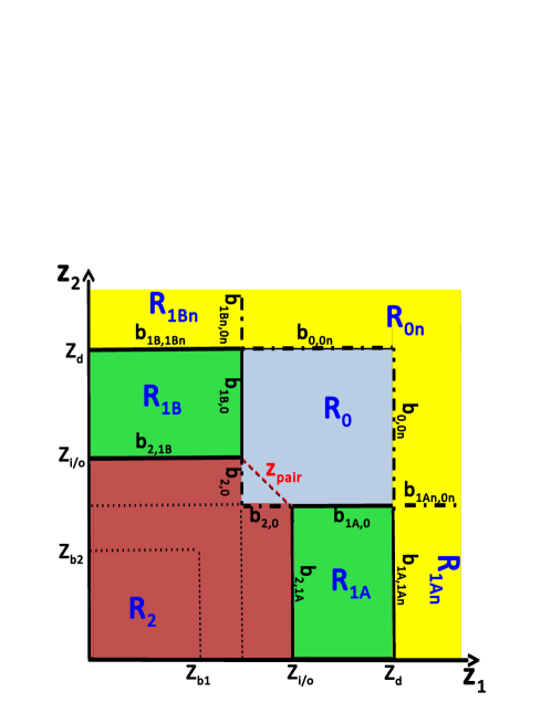
Figure 5: (Color online) Configuration space of the two-particle system. The regions $R_{j}$ ($j=2,1A,1B,0,1An,1Bn,0n$) are shown in different colors/shades. Each region $R_{j}$ is surrounded by the boundary $B_{j}$ (not shown). Boundary segments that divide regions $R_{j}$ and $R_{j^{\prime}}$ are labeled by $b_{j,j^{\prime}}$. $z_{b1}$ and $z_{b2}$ denote the position of the maximum of the barrier at $t=-t_{r}$. $z_{\text{i}/\text{o}}$ divides the “inside” from the “outside”; we choose $z_{\text{i}/\text{o}}$ to be larger than $z_{b1}$ and $z_{b2}$ to ensure that the calculated flux is independent of how it is extracted. $z_{\text{d}}$ denotes the largest $z_{1}$ and $z_{2}$ for which we calculate the “physical” wave packet. $z_{\text{pair}}$ is equal to $2a_{\text{1D}}$ for the molecular branch and equal to $2a_{\text{ho}}$ for the upper branch; $z_{\text{pair}}$ enters into our analysis of the pair tunneling (see text for details).

Region $R_{2}$ corresponds to the situation where two particles are in the trap, region $R_{0}$ corresponds to the situation where both particles have left the trap, and region $R_{1A}$ ($R_{1B}$) corresponds to the situation where particle 1 (2) has left the trap while particle 2 (1) is in the trap. The regions $R_{1An}$, $R_{1Bn}$, and $R_{0n}$ correspond to numerical regions in which we apply damping (see below). The region $R_{j}$ is encircled by the boundary $B_{j}$ (the $B_{j}$’s are not labeled in Fig. 5). To analyze the flux, the boundaries $B_{j}$ are broken up into boundary segments $b_{j,j^{\prime}}$ that border regions $R_{j}$ and $R_{j^{\prime}}$.

The flux through boundaries $b_{2,1A}$ and $b_{2,1B}$ is interpreted as uncorrelated single-particle tunneling while the flux through boundary $b_{2,0}$ is interpreted as pair tunneling. The pair tunneling rate extracted from the flux through $b_{2,0}$ is not unique and depends on $z_{\text{pair}}$. Section III.2 considers $1.1a_{\text{ho}}<a_{\text{1D}}<4.5a_{\text{ho}}$; motivated by the fact that the size of the free space molecule is approximately $a_{1\text{D}}$ footnote (6), we use $z_{\text{pair}}=2a_{1\text{D}}$ for this $a_{1\text{D}}$ range. For the upper branch simulations, we use $z_{\text{pair}}=2a_{\text{ho}}$. We found that the flux through $b_{2,0}$ is vanishingly small for the upper branch simulations. We set $z_{\text{i/o}}$, which defines where the “inside” region ends and the “outside” region starts, such that $z_{\text{i/o}}>\max(z_{b1},z_{b2})$. For the molecular branch simulations, the flux dynamics is quite complex near the top of the barrier. To be independent of the “near-field” dynamics, we choose $z_{\text{i/o}}\approx 15a_{\text{ho}}$ and $13a_{\text{ho}}$ for the molecular branch and upper branch, respectively. The physical regions end at $z_{\text{d}}$, i.e., for $z_{1}>z_{\text{d}}$ or $z_{2}>z_{\text{d}}$ a damping function is applied. The damping function acts like an absorbing boundary (see Appendix F). The damping function is needed since the flux reaches the end of the simulation box within a small fraction of the total simulation time. $z_{\text{d}}$ has to be so large that the two particles are essentially uncorrelated for $z>z_{\text{d}}$. In practice we vary $z_{\text{d}}$ and choose its value such that the observables do not change as $z_{\text{d}}$ is increased. Typical values for $z_{\text{d}}$ are $25a_{\text{ho}}$ for the molecular branch simulations and $13a_{\text{ho}}$ for the upper branch simulations (for the upper branch, we found that $z_{\text{d}}=z_{\text{i/o}}$ yields the same results as $z_{\text{d}}>z_{\text{i/o}}$). As mentioned above, the time-dependent simulation starts at $t=-t_{r}$, where the probability $P_{2}(-t_{r})$ to find two particles in the trap (i.e., in region $R_{2}$) equals 1. For $t>t_{r}$, $P_{2}(t)$ decays with time. This decay, except for a short period of time ($t\lesssim 20$ms), is well described by the exponential function

$$P_{2}(t)=P_{2}(t_{\text{ref}})\exp[-\gamma_{2}(t-t_{\text{ref}})],$$ (14)

where $\gamma_{2}$ denotes the decay rate. Since both uncorrelated single-particle tunneling and pair tunneling can contribute to the change of $P_{2}(t)$, we break $\gamma_{2}$ into two pieces, $\gamma_{2}=\gamma_{\text{s}}+\gamma_{\text{P}}$, where $\gamma_{\text{s}}$ and $\gamma_{\text{P}}$ denote the single-particle tunneling and pair tunneling contributions, respectively (see Appendix G for details). A non-zero $\gamma_{\text{s}}$ means that the probability $P_{1}(t)$ to find one particle in the trap is finite. We also define the mean number $\bar{N}$ of trapped particles,

$$\bar{N}(t)=2P_{2}(t)+P_{1}(t).$$ (15)

The time dependence of $\bar{N}(t)$ is approximately parameterized by an exponential decay with tunneling rate $\gamma$,

$$\bar{N}(t)=\bar{N}(t_{\text{ref}})\exp[-\gamma(t-t_{\text{ref}})]+C,$$ (16)

where $C$ denotes a constant. Subsections III.2 and IV.2 present the results of our time-dependent two-particle simulations.

III Molecular branch tunneling dynamics

III.1 Single-particle tunneling dynamics and trap calibration

In the following we perform exact numerical calculations for the trap parameters reported in Table 1. We will show that the numerically obtained tunneling rates do not agree with the measured ones and propose an alternative calibration approach.

The trap employed in the molecular branch experiments was calibrated, in addition to the calibration experiments already discussed in Sec. II, based on four single-particle experiments Zürn et al. (2013a) [see Table 2 and diamonds in Figs. 6(a) and  6(b)].

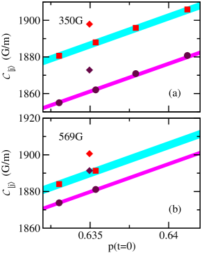
Figure 6: (Color online) Parameter combinations ($p(t=0),\mathcal{C}_{|j\rangle}(B)$) that reproduce the experimentally measured single-particle tunneling rates at (a) $B=350$G and (b) $569$G. For all calculations, $z_{\text{R}}=9.975\mu$m is used. In panels (a) and (b), the initial state corresponds to the trap ground state. The bands show the parameter combinations for which our full time-dependent calculations reproduce the experimentally measured tunneling rates. The widths of the bands originate from the experimental error bars Zürn et al. (2013a). In panels (a) and (b), the dark (magenta) and light (cyan) bands correspond to ⁶Li atoms in states $|1\rangle$ and $|3\rangle$, respectively. Circles and squares show parameter combinations for states $|1\rangle$ and $|3\rangle$, respectively, that are used in the two-particle calculations (see Sec. III.2). For comparison, the diamonds show the ($p(t=0)$, $\mathcal{C}_{|j\rangle}(B)$) pairs that were suggested in Ref. Zürn et al. (2013a).

In our first calculation, we use $\mathcal{C}_{|1\rangle}=1872.87$G/m, corresponding to $c_{|1\rangle}=0.98989$ and $B^{\prime}=1892$G/m, and prepare the system in the trap ground state [see the diamond in Fig. 6(a)]. The dashed line in Fig. 7

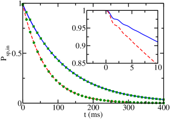
Figure 7: (Color online) Single-particle tunneling as a function of time for a ⁶Li atom in state $|1\rangle$ at $B=350$G in the trap ground state. The dashed and solid lines show the probability $P_{\text{sp,in}}(t)$ of finding the particle in the trap calculated using the exact time evolution for $p(t=0)=0.63496$ and $\mathcal{C}_{|1\rangle}=1872.87$G/m ($c_{|1\rangle}=0.98989$ and $B^{\prime}=1892$G/m) (these parameters are proposed in Ref. Zürn et al. (2013a)) and for $p(t=0)=0.63536$ and $\mathcal{C}_{|1\rangle}=1862.03$G/m (this is one of many parameter sets that reproduces the experimentally measured tunneling rate), respectively. The time evolution starts at $-t_{r}$ ($t_{r}\approx 3.72\text{ms}$ and $t_{r}\approx 3.71\text{ms}$ for the dashed and solid lines, respectively). Circles and squares show exponentially decaying functions [see Eq. (5)] with $\gamma_{\text{sp}}=15.39\text{s}^{-1}$ and $\gamma_{\text{sp}}=8.28\text{s}^{-1}$, respectively. The inset shows a blow-up of the short-time behavior.

shows the result of our simulation for $p(0)=0.63496$. A fit of our data for $t>15$ms (the short-time dynamics exhibits, as can be seen in the inset of Fig. 7, oscillations) to Eq. (5) yields $\gamma_{\text{sp}}^{\text{num}}=15.39\text{s}^{-1}$ (see circles in Fig. 7). The tunneling rate $\gamma_{\text{sp}}^{\text{num}}$ obtained from the real time propagation is nearly twice as large as the experimentally measured tunneling rate $\gamma_{\text{sp}}^{\text{exp}}$, $\gamma_{\text{sp}}^{\text{exp}}=8.28(0.49)\text{s}^{-1}$ Zürn et al. (2013a). This means that the trap parameters reported in Ref. Zürn et al. (2013a), obtained through the WKB analysis, yield a tunneling rate that deviates by a factor of nearly $2$ from the experimentally measured tunneling rate, $\gamma_{\text{sp}}^{\text{num}}/\gamma_{\text{sp}}^{\text{exp}}=1.86$. To understand this, we treat $t_{r}$ as a parameter. Our tunneling simulations indicate that the exact shape of the initial state, and thus $p(-t_{r})V_{0}$, has a very small effect on the tunneling rate. The tunneling rate, in contrast, depends appreciably on the value of $p(0)V_{0}$. Thus, changing $t_{r}$ while keeping $p(-t_{r})V_{0}$ fixed at $0.795V_{0}$ has a similar effect to changing $V_{0}$. Solid and dotted lines in Fig. 8

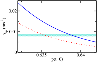
Figure 8: (Color online) Tunneling rate of a ⁶Li atom at $B=350$G as a function of the dimensionless parameter $p(t=0)$. The atom is prepared in the ground state of the trap, and $c_{|1\rangle}=0.98989$ and $B^{\prime}=1892$G/m are used. The solid and dotted lines show the tunneling rates obtained through exact time propagation and the WKB approximation, respectively. The horizontal band shows the tunneling rate $\gamma_{\text{sp}}^{\text{exp}}=8.28(0.49)\text{s}^{-1}$ measured experimentally Zürn et al. (2013a) (the width of the band represents the experimental error bar).

show the numerically determined tunneling rate $\gamma_{\text{sp}}^{\text{num}}$ and the WKB tunneling rate $\gamma_{\text{sp}}^{\text{WKB}}$ as a function of $p(t=0)$, i.e., for varying $t_{r}$ (using $c_{|1\rangle}=0.98989$ and $B^{\prime}=1892$G/m Zürn et al. (2013a)). It can be seen that the WKB analysis yields tunneling rates that differ by a factor of about 1/2 from those obtained from the full time evolution. This is elaborated on further in Appendix H. Since the trap parameters reported by the experimental group utilized the WKB approximation, we conclude that the trap parameters reported in Table 1 are inaccurate. Table 2

Table 2: Experimentally measured single-particle tunneling rates $\gamma_{\text{sp}}^{\text{exp}}$ for selected magnetic field strengths and initial single-particle states relevant to the molecular branch experiments Zürn et al. (2013a). Column 4 reports the values of the dimensionless coefficients $c_{|j\rangle}(B)$ reported in Ref. Zürn et al. (2013a). The fifth column reports the tunneling rate $\gamma_{\text{sp}}^{\text{num}}$ obtained from the exact time evolution using the trap parameters listed in Table 1. As shown in column 6, the exact time evolution yields tunneling rates that are inconsistent with $\gamma_{\text{sp}}^{\text{exp}}$, suggesting that the trap calibration that involves the WKB analysis needs to be refined.

state $|j\rangle$	$B$ (G)	$\gamma_{\text{sp}}^{\text{exp}}$ ($\text{s}^{-1}$)	$c_{|j\rangle}(B)$	$\gamma_{\text{sp}}^{\text{num}}$ ($\text{s}^{-1}$)	$\gamma_{\text{sp}}^{\text{num}}/\gamma_{\text{sp}}^{\text{exp}}$
$|1\rangle$ trap’s gr. st.	$350$	$8.28(0.49)$	$0.98989$	$15.39$	$1.86$
$|3\rangle$ trap’s gr. st.	$350$	$30.12(2.81)$	$1.00311$	$50.24$	$1.67$
$|1\rangle$ trap’s gr. st.	$569$	$21.76(1.12)$	$0.99968$	$37.36$	$1.72$
$|3\rangle$ trap’s gr. st.	$569$	$35.25(3.57)$	$1.00457$	$55.87$	$1.58$

compares the measured tunneling rates $\gamma_{\text{sp}}^{\text{exp}}$ with the numerically calculated tunneling rates $\gamma_{\text{sp}}^{\text{num}}$ for the trap parameters summarized in Table 1 and the $c_{|j\rangle}$ coefficients listed in Table 2.

The bands in Figs. 6(a) and 6(b) show the $(p(t=0),\mathcal{C}_{|j\rangle})$ values for state $|1\rangle$ [darker (magenta) band] and state $|3\rangle$ [lighter (cyan) band] for which the $\gamma_{\text{sp}}^{\text{num}}$ agree with the experimentally measured single-particle tunneling rates for states $|1\rangle$ and $|3\rangle$. In our calculations, the initial state corresponds to the lowest trap state. In a first attempt, we did set $c_{|j\rangle}(B)=c_{|j\rangle}^{\text{BR}}(B)$ and aimed to find unique values for $p(t=0)$ and $B^{\prime}$ that would reproduce all four experimentally measured tunneling rates. For the functional form of the potential (with the parameters $V_{0}$, $z_{\text{R}}$, $B^{\prime}$, and $dp/dt$ from Table 1), such a parameter combination does not exist. Allowing $z_{\text{R}}$ to vary does not change the situation. To reproduce the experimentally measured tunneling rates, we thus decided to treat $\mathcal{C}_{|j\rangle}(B)$ as a free parameter. For example, we set $c_{|3\rangle}(569\text{G})=c_{|3\rangle}^{\text{BR}}(569\text{G})$ and $B^{\prime}=1890$G/m and determine $p(t=0)$ such that we reproduce the experimental single-particle rate. We find $p(t=0)=0.63536$. We then set $p(t=0)$ to $0.63536$ and find $c_{|1\rangle}(569\text{G})$, $c_{|1\rangle}(350\text{G})$, and $c_{|3\rangle}(350\text{G})$ such that $\gamma_{\text{sp}}^{\text{num}}=\gamma_{\text{sp}}^{\text{exp}}$ [see squares and circles in Figs. 6(a) and 6(b)]. We emphasize that these are not unique parameter combinations. Alternative parameter combinations that are also used in Sec. III.2 are marked in Figs. 6(a) and 6(b).

To obtain the $\mathcal{C}_{|j\rangle}(B)$ coefficients for other magnetic fields, we use interpolations/extrapolations. For state $|1\rangle$, we use

$$c_{|1\rangle}(B)\approx c_{0}+\frac{c_{-1}}{B}+\frac{c_{-2}}{B^{2}}$$ (17)

with $c_{0}=1.00338$, $c_{-1}=-1.89121$G, and $c_{-2}=-1565.12\text{G}^{2}$. This functional form (i) reproduces $c_{|1\rangle}(350\text{G})=0.985202$ and $c_{|1\rangle}(569\text{G})=0.995224$ and (ii) is designed such that the functional dependence of $c_{|1\rangle}(B)$ is similar to that of $c_{|1\rangle}^{\text{BR}}(B)$. For state $|3\rangle$, we use $c_{|3\rangle}(B)=c_{|3\rangle}(569\text{G})$ for $B\geq 569$G and a linear interpolation for $350\text{G}\leq B\leq 569$G using the known $c_{|3\rangle}$ values at 350G and 569G. Table 3 summarizes the parameters that are used in Sec. III.2 to model the two-particle experiments.

III.2 Two-particle tunneling dynamics

This section considers two attractively-interacting ⁶Li atoms in hyperfine states $|1\rangle$ and $|3\rangle$ on the molecular branch. As discussed in Sec. II.3, the one-dimensional coupling constant $g_{1\text{D}}$ depends on $p(t)$. Specifically, $g_{1{\text{D}}}$ changes for $t=-t_{r}$ to $t=0$ and is constant for $t=0$ to $t=t_{\text{hold}}$. While this time dependence can be incorporated straightforwardly into the finite-range simulations (in this case, the depth $V_{\text{G}}$ can be made to vary with time), incorporating the time dependence into the zero-range calculations is more involved since $g_{1\text{D}}$ enters into the propagator. To estimate the importance of the time dependence during the initial down ramp (time $t=-t_{r}$ to $0$), we compared the simulation results for the cases where the full time dependence of $g_{1\text{D}}$ was accounted for [i.e., $\omega_{\rho}$ was calculated according to $\sqrt{p(t)}\omega_{\rho}^{\text{ref}}$] and where the time dependence was neglected [i.e., $\omega_{\rho}$ was calculated according to $\sqrt{p(0)}\omega_{\rho}^{\text{ref}}$] for selected magnetic field strengths. We found that the difference between the resulting tunneling rates is between $0.02$% and $0.2$%. Since this difference is much smaller than the difference between our calculated tunneling rates and the experimentally measured tunneling rates (see below), the time dependence of $g_{1{\text{D}}}$ is neglected in what follows. The reason why the tunneling rates, calculated by accounting for and neglecting the time dependence of $g_{1\text{D}}$, are so similar is two-fold. First, very little tunneling occurs during the down ramp. Second, the overlap between the states at $t=-t_{r}$ with somewhat different $g_{1\text{D}}$ is much larger than the overlap between the states at $t=-t_{r}$ and $t=0$. This implies that the down ramp has a much larger effect on the state that results at $t=0$ than a small variation of $g_{1\text{D}}$ during the down ramp.

The top panel in Fig. 9

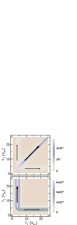
Figure 9: (Color online) Probability flux $|{\bf{j}}(z_{1},z_{2},t)|$. The top and bottom panels show the probability flux at $t=98$ms for two distinguishable particles with $g_{1\text{D}}=-1.451E_{\text{ho}}a_{\text{ho}}$ and $g_{1\text{D}}=0$, respectively (the trap parameters are given, respectively, in the sixth and first rows of Table 3). The values of the flux are shown in the legend on the right in units of $\omega/a_{\text{ho}}$ (note the different scales for the top and bottom panels). The arrows indicate the primary directions of the flux ${\bf{j}}$.

shows the magnitude $|{\bf{j}}(z_{1},z_{2},t)|$ of the flux for $g_{1\text{D}}=-1.451E_{\text{ho}}a_{\text{ho}}$ [corresponding to $a_{1\text{D}}/a_{\text{ho}}=1.378$ ($B=1202$G, see Table 3)] at $t=98$ms. As can be seen (see also the arrows in the top panel of Fig. 9), the flux density is maximal along $z_{1}\approx z_{2}$. Only a small portion of the flux is directed along the $\hat{\bf{z}}_{1}$ or $\hat{\bf{z}}_{2}$ directions. This demonstrates that pair tunneling becomes dominant for sufficiently strong interactions. For comparison, the bottom panel of Fig. 9 shows the quantity $|{\bf{j}}(z_{1},z_{2},t)|$ for the same $t$ but $g_{1\text{D}}=0$. In this case pair tunneling is absent. A careful comparison of the flux in the $\hat{\bf{z}}_{1}$ and $\hat{\bf{z}}_{2}$ directions shows that the flux along $\hat{\bf{z}}_{2}$ is notably larger, reflecting the fact that the trap felt by particle 2 (parameterized via $\mathcal{C}_{|3\rangle}$) is shallower than the trap felt by particle 1 (parameterized via $\mathcal{C}_{|1\rangle}$). We note that the flux has a very intricate structure in the vicinity of the barrier, especially in the upper panel, that is not visible on the scale of Fig. 9. Unlike the flux plots shown in Fig. 3 of Ref. Lundmark et al. (2015), we do not observe “wave-like patterns” overlaying the flux. We speculate that these features are artifacts of the numerics of Ref. Lundmark et al. (2015).

Figure 10 summarizes the tunneling rates obtained from our full time-dependent molecular branch simulations for finite-range interactions. To obtain these results, $\omega_{\rho}$ (and hence $g_{1{\text{D}}}$) was calculated according to $\omega_{\rho}=\sqrt{p(t=0)}\omega_{\rho}^{\text{ref}}$. Squares in Fig. 10(a) show the inverse of $\gamma_{2}$, i.e., the inverse of the rate with which the probability $P_{2}(t)$ to find both particles in the trap decays, using the trap parameters that reproduce the experimentally measured single-particle tunneling rates. As can be seen, the squares lie notably above the experimentally measured $(\gamma_{2}^{\text{exp}})^{-1}$ for finite $g_{1\text{D}}$; for $g_{1\text{D}}=0$, the simulation results and the experimentally measured rate agree by construction since the single-particle tunneling rates in this case add up to $\gamma_{2}$ (see also Table 3).

Table 3: Molecular branch dynamics for two distinguishable particles in states $|1\rangle$ and $|3\rangle$ for various magnetic field strengths. The second column reports the one-dimensional coupling constant $g_{1\text{D}}$ calculated using $\omega_{\rho}=\sqrt{p(0)}\omega_{\rho}^{\text{ref}}$. The third column indicates whether the simulation results were obtained using the zero-range interaction model (ZR) or the gaussian interaction model with $z_{0}=0.2a_{\text{ho}}$ (FR). Columns 4 and 5 report the $\mathcal{C}_{|j\rangle}$ coefficients for the trap parameterization with $p(t=0)=0.63536$ (see Sec. II) and $z_{\text{R}}=8.548a_{\text{ho}}$. Column 6 reports the tunneling rate $\gamma_{2}^{\text{num}}$ [see Eq. (14)] obtained from our full time-dependent simulations. For comparison, column 7 shows the experimentally measured tunneling rates with error bars footnote (5). Column 8 shows the rate $\gamma_{2}^{\text{TI}}$ obtained from time-independent simulations Lundmark et al. (2015).

$B$ (G)	$g_{1\text{D}}$ $(a_{\text{ho}}E_{\text{ho}})$	ZR/FR	$\mathcal{C}_{|1\rangle}$ (G/m)	$\mathcal{C}_{|3\rangle}$ (G/m)	$\gamma_{2}^{\text{num}}$ ($\text{s}^{-1}$)	$\gamma_{2}^{\text{exp}}$ ($\text{s}^{-1}$) footnote (5)	$\gamma_{2}^{\text{TI}}$ ($\text{s}^{-1}$) Lundmark et al. (2015)
$569$	$0$	—	$1881.11$	$1891.32$	$57.0$	$57.01(3.74)$	—
$496$	$-0.446$	ZR	$1877.16$	$1890.19$	$13.8(0.3)$	$22.2(1.0)$	$19.2(0.5)$
$496$	$-0.446$	FR	$1877.16$	$1890.19$	$14.0$	$22.2(1.0)$	$19.2(0.5)$
$423$	$-0.601$	FR	$1871.41$	$1889.06$	$6.67$	$13.84(1.04)$	$12.5(0.5)$
$350$	$-0.654$	FR	$1862.03$	$1887.93$	$4.27$	$9.70(0.33)$	$25.8(0.5)$
$1202$	$-1.451$	FR	$1891.38$	$1891.32$	$0.360$	$2.14(0.19)$	$0.4(0.5)$
$1074$	$-1.503$	FR	$1890.49$	$1891.32$	$0.293$	$1.931(0.123)$	—
$958$	$-1.595$	FR	$1889.44$	$1891.32$	$0.216$	$1.227(0.053)$	—
$851$	$-1.797$	FR	$1888.11$	$1891.32$	$0.137$	$0.505(0.023)$	—

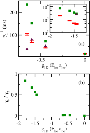
Figure 10: (Color online) Molecular branch tunneling dynamics for two distinguishable particles as a function of $g_{1\text{D}}$. The coupling constant is calculated using $\omega_{\rho}=\sqrt{p(0)}\omega_{\rho}^{\text{ref}}$. (a) The squares show the results from our full time-dependent simulations using the trap parameters given in Table 3; these trap parameters yield single-particle tunneling rates $\gamma_{\text{sp}}^{\text{num}}$ that agree with the experimentally measured single-particle tunneling rates $\gamma_{\text{sp}}^{\text{exp}}$. The symbols with error bars show the experimental results footnote (5). For comparison, the triangles show the simulation results from Ref. Lundmark et al. (2015). The inset shows the strongly-attractive region using the same symbols as in the main figure but a logarithmic $y$-scale. (b) Squares show the ratio $\gamma_{\text{P}}/\gamma_{2}$ obtained from our full time-dependent simulations.

Table 4: Molecular branch dynamics for two distinguishable particles in states $|1\rangle$ and $|3\rangle$ for various magnetic field strengths. The second column reports the one-dimensional coupling constant $g_{1\text{D}}$ calculated using $\omega_{\rho}=0.67\sqrt{p(0)}\omega_{\rho}^{\text{ref}}$. The calculations are performed using the gaussian interaction model with $z_{0}=0.2a_{\text{ho}}$ and the trap parameters are the same as those for the calculations reported in Table 3. Column 3 reports the tunneling rate $\gamma_{2}^{\text{num}}$ [see Eq. (14)] obtained from our full time-dependent simulations.

$B$ (G)	$g_{1\text{D}}$ ($E_{\text{ho}}a_{\text{ho}}$)	$\gamma_{2}^{\text{num}}$ ($s^{-1}$)
$496$	$-0.303$	$22.4$
$423$	$-0.410$	$13.4$
$350$	$-0.447$	$9.57$
$1202$	$-1.018$	$1.89$
$1074$	$-1.056$	$1.53$
$958$	$-1.124$	$1.04$
$851$	$-1.275$	$0.62$

The molecular branch tunneling dynamics has previously been calculated by Lundmark et al. using a time-independent method Lundmark et al. (2015). Unfortunately, the trap parameters used to perform the calculations were not reported. The triangles in Fig. 10(a) show the result of this study. It can be seen that the inverse tunneling rate $(\gamma_{2}^{\text{num}})^{-1}$ is a non-monotonic function of $g_{1\text{D}}$; such non-monotonic behavior is not displayed in our simulations. Reference Lundmark et al. (2015) interpreted the non-monotonic dependence as an interplay between the trap parameters.

To quantify the contribution of pair tunneling, we break $\gamma_{2}$ into two parts, $\gamma_{2}=\gamma_{\text{P}}+\gamma_{\text{s}}$, where $\gamma_{\text{P}}$ is the pair tunneling rate and $\gamma_{\text{s}}$ the single-particle tunneling rate. We identify these rates from the flux passing through the boundary $b_{2,0}$ and the sum of the fluxes passing through the boundaries $b_{2,1A}$ and $b_{2,1B}$. Figure 10(b) shows the ratio $\gamma_{\text{P}}/\gamma_{2}$ as a function of the interaction strength. We find that $\gamma_{\text{P}}$ is approximately equal to $0$ for $g_{1\text{D}}\geq-0.654E_{\text{ho}}a_{\text{ho}}$. As one might predict intuitively, the ratio $\gamma_{\text{P}}/\gamma_{2}$ increases to close to 1 for stronger attractive interactions. In this regime, the molecule can be treated as a point particle of mass $2m$. Our simulation results for $g_{1\text{D}}\geq-0.654E_{\text{ho}}a_{\text{ho}}$ are consistent with the experimental observation of negligibe pair tunneling. In the strongly-interacting regime, i.e., for $g_{1\text{D}}\leq-1.451E_{\text{ho}}a_{\text{ho}}$, the experiments could not resolve the pair versus single-particle tunneling fractions.

To understand why our finite-$g_{1\text{D}}$ simulations predict larger tunneling constants $1/\gamma_{2}$ than measured experimentally [see Fig. 10(a)], we repeated our simulations using several possible parameter sets that reproduce the experimentally measured single-particle tunneling rates, marked on the bands in Fig. 6. We found that the two-body results remain almost unchanged, suggesting that the non-uniqueness of the trap parameterization is not the cause for the disagreement. We also repeated one calculation using the zero-range interaction model as opposed to the finite-range interaction model (see Table 3). Again, we found that the result remains almost unchanged, suggesting that finite-range effects are not the cause for the disagreement. As a third possibility we investigated the dependence of the tunneling rates on $\omega_{\rho}$. As we now show, a smaller $\omega_{\rho}$ brings the tunneling rates obtained from the full time-dependent simulations in pretty good agreement with the experimentally measured tunneling rates.

As discussed in Sec. II.3 the magnetic field gradient pushes the particles out to finite positive $z$, resulting in, on average, a weaker confinement along the tight confinement direction. Squares in Fig. 11 show $1/\gamma_{2}$, obtained from our full time-dependent simulations, using the trap parameters that reproduce the experimentally measured single-particle tunneling rates and $g_{1{\text{D}}}$ calculated according to $\omega_{\rho}=0.67\sqrt{p(t=0)}\omega_{\rho}^{\text{ref}}$ (see also Table 4).

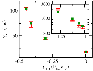
Figure 11: (Color online) Molecular branch tunneling dynamics for two distinguishable particles as a function of $g_{1\text{D}}$. The coupling constant is calculated using $\omega_{\rho}=0.67\sqrt{p(0)}\omega_{\rho}^{\text{ref}}$. The squares show the results from our full time-dependent simulations using the trap parameters given in Table 3; these trap parameters yield single-particle tunneling rates $\gamma_{\text{sp}}^{\text{num}}$ that agree with the experimentally measured single-particle tunneling rates $\gamma_{\text{sp}}^{\text{exp}}$. The symbols with error bars show the experimental results footnote (5). The inset shows the strongly-attractive region using the same symbols as in the main figure but a logarithmic $y$-scale.

The factor of $0.67$ yields (roughly) maximal agreement between the time constants obtained from our simulations and those measured experimentally (symbols with error bars in Fig. 11). Recalling the discussion presented in Sec. II.3, this value seems reasonable, though possibly slightly smaller than one might have expected naively. While other explanations for the disagreement between the squares and the symbols with error bars in Fig. 10(a) cannot be ruled out, our results indicate that the addition of the magnetic field gradient may have a non-trivial effect on the calculation of the renormalized one-dimensional coupling constant $g_{1{\text{D}}}$.

IV Upper branch tunneling dynamics

IV.1 Trap calibration

As discussed in Sec. II, the trap used in the upper branch experiment was calibrated by preparing two identical non-interacting fermions in state $|2\rangle$ at various magnetic field strengths. The measured tunneling rates $\gamma^{\text{exp}}$ were obtained by fitting $\bar{N}(t)$ to an exponential plus a constant. Table 5

Table 5: Upper branch dynamics for two distinguishable particles in states $|1\rangle$ and $|2\rangle$ for various magnetic field strengths. The second column reports the one-dimensional coupling constant $g_{1\text{D}}$ calculated using $\omega_{\rho}=\sqrt{p(0)}\omega_{\rho}^{\text{ref}}$. The third column indicates whether the simulation results were obtained using the zero-range interaction model (ZR) or the gaussian interaction model with $z_{0}=0.2a_{\text{ho}}$ (FR). Columns 4 and 5 report the $\mathcal{C}_{|j\rangle}$ coefficients; as discussed in Sec. IV.1, we use $c_{|j\rangle}=c_{|j\rangle}^{\text{BR}}$, $B^{\prime}=1890$G/m, $p(t=0)=0.68$, and $z_{\text{R}}=8.548a_{\text{ho}}$. Column 6 reports the tunneling rate $\gamma^{\text{num}}$ [see Eq. (16)] obtained from our full time-dependent simulations. For comparison, column 7 shows the experimentally measured tunneling rates with error bars footnote (11).

$B$ (G)	$g_{1\text{D}}$ ($a_{\text{ho}}E_{\text{ho}}$)	ZR/FR	$\mathcal{C}_{|1\rangle}$ (G/m)	$\mathcal{C}_{|2\rangle}$ (G/m)	$\gamma^{\text{num}}$ ($\text{s}^{-1}$)	$\gamma^{\text{exp}}$ ($\text{s}^{-1}$)
$750$	$6.15$	ZR	$1883.86$	$1881.60$	$4.2(0.5)$	$2.9(0.2)$
$782$	$\infty$	ZR	$1884.56$	$1882.47$	$15$	$12.8(1.2)$
$855$	$-4.42$	FR	$1885.88$	$1884.07$	$77$	$62.8(8.2)$
$900$	$-3.15$	ZR	$1886.57$	$1884.90$	$127$	$107(12)$
$900$	$-3.15$	FR	$1886.57$	$1884.90$	$130$	$107(12)$

summarizes $\gamma^{\text{exp}}$ footnote (11). To see if the trap parameterization proposed by the experimental group is accurate, we perform a time-dependent two-particle simulation for the anti-symmetrized two-particle wave packet using the trap parameters reported in Table 1 and $c_{|2\rangle}=1$. We find $\gamma^{\text{num}}=6.86\text{s}^{-1}$, which is about two times smaller than the experimentally measured value, i.e., $\gamma^{\text{num}}/\gamma^{\text{exp}}\approx 0.5$ (note, this ratio is around 1.7 for the molecular branch; see Sec. III.1 and Appendix H). Similar to the molecular branch, we conclude that the WKB approximation cannot be used to calibrate the trap.

To recalibrate the trap, we set $c_{|2\rangle}=c_{|2\rangle}^{\text{BR}}$ and adjust $p(t=0)$ and $B^{\prime}$ such that $\gamma^{\text{num}}$ for the anti-symmetric two-particle state at $B=782$G agrees, within error bars, with the experimentally measured tunneling rate. As in the molecular branch (see Fig. 6), we do not find a unique parameter combination but a parameter band. Using $p(t=0)=0.68$, $B^{\prime}=1890$G and $c_{|2\rangle}=c_{|2\rangle}^{\text{BR}}$, we find the tunneling rate $\gamma^{\text{num}}$ for several magnetic field strengths (see Table 6).

Table 6: Tunneling dynamics for two identical particles in state $|2\rangle$ for various magnetic field strengths. The second column reports the $\mathcal{C}_{|j\rangle}$ coefficients; as discussed in Sec. IV.1, we use $c_{|j\rangle}=c_{|j\rangle}^{\text{BR}}$, $B^{\prime}=1890$G/m, $p(t=0)=0.68$, and $z_{\text{R}}=8.548a_{\text{ho}}$. Column 3 reports the tunneling rate $\gamma^{\text{num}}$ [see Eq. (16)] obtained from our full time-dependent simulations. For comparison, column 4 shows the experimentally measured tunneling rate $\gamma^{\text{exp}}$ with error bars footnote (11).

$B$ (G)	$\mathcal{C}_{|2\rangle}$ (G/m)	$\gamma^{\text{num}}$ ($\text{s}^{-1}$)	$\gamma^{\text{exp}}$ ($\text{s}^{-1}$)
$750$	$1881.60$	$13.2$	$14.7(1.3)$
$782$	$1882.47$	$13.8$	$13.2(1.1)$
$820$	$1883.37$	$14.5$	$13.1(1.4)$
$855$	$1884.07$	$15.1$	$11.5(1.3)$
$900$	$1884.90$	$15.8$	$16.0(1.1)$

Our $\gamma^{\text{num}}$ agree with $\gamma^{\text{exp}}$ within error bars, except for the cases at $B=750$G and $B=855$G, where the deviations are, respectively, about $1.1$ and $2.5$ times larger than the error bars.

IV.2 Two-particle tunneling dynamics

This section discusses the upper branch tunneling dynamics for two distinguishable particles with finite interaction strength $g_{1{\text{D}}}$. Solid and dashed lines in Fig. 12(a) show the mean number of trapped particles $\bar{N}$, Eq. (15), extracted from our full time-dependent simulations as a function of the hold time for two distinguishable particles at $B=782$G ($g_{\text{1D}}=192a_{\text{ho}}E_{\text{ho}}$; in what follows, we use $g_{1{\text{D}}}=\infty$ for this magnetic field strength) and $B=900$G ($g_{\text{1D}}=-3.15a_{\text{ho}}E_{\text{ho}}$). Here, $g_{1{\text{D}}}$ is calculated using $\omega_{\rho}=\sqrt{p(t=0)}\omega_{\rho}^{\text{ref}}$. As can be seen in Fig. 4, the upper branch energy of the quasi-eigenstate at $t=-t_{\text{r}}$ is larger for negative $g_{\text{1D}}$ than for infinitely large $g_{\text{1D}}$. This implies that the effective barrier height that the two-particle system sees is smaller at $B=900$G than at $B=782$G, resulting in faster tunneling dynamics for the system at $B=900$G than at $B=782$G. The tunneling rates $\gamma$, obtained by fitting our data to Eq. (16) or from the flux analysis (see Appendix G), are $\gamma^{\text{num}}=127\text{s}^{-1}$ for $B=900$G and $\gamma^{\text{num}}=15\text{s}^{-1}$ for $B=782$G. These tunneling rates agree at the two sigma level with the experimentally measured rates of $\gamma^{\text{exp}}=107(12)\text{s}^{-1}$ [see triangles in Fig. 12(a)] and $12.8(1.2)\text{s}^{-1}$ footnote (11) [see squares in Fig. 12(a)].

An important aspect of the tunneling dynamics of the upper branch is that the mean number of trapped particles $\bar{N}$ decreases from 2 to approximately 1 over the hold times considered. This suggests that the particle that remains trapped has such a small energy that its tunneling dynamics is orders of magnitude slower than the tunneling dynamics considered in Fig. 12. Indeed, we observe essentially no flux through the boundaries $b_{1A,0}$ and $b_{1B,0}$. Comparing the portion of the wave packet in region $R_{1A}$ (or $R_{1B}$) with the quasi-eigenstate of a single trapped particle shows that the remaining particle occupies to a good approximation the lowest trap state. This implies that the particle that leaves the trap carries away the “excess energy”. Performing single-particle calculations for particles $|1\rangle$ and $|2\rangle$ initially in the trap ground state, we find tunneling rates of 0.008s^-1 and 0.007s^-1. This confirms the separation of time scales alluded to above.

Circles in Fig. 12(b) show our tunneling time constants $(\gamma^{\text{num}})^{-1}$ for two distinguishable particles as a function of the magnetic field strength. Our $(\gamma^{\text{num}})^{-1}$ follow the overall trend of the experimentally measured $(\gamma^{\text{exp}})^{-1}$ [diamonds in Fig. 12(b)] but lie a bit lower (see also Table 5). The discrepancy is largest for positive $g_{\text{1D}}$ ($B=750$G), where the dynamics is slowest. This is the regime where our simulations are, due to the slow tunneling, the most demanding. We estimate, however, that our numerical uncertainties do not account for the $45\%$ discrepancy between the calculated tunneling constant $(\gamma^{\text{num}})^{-1}$ and the experimentally measured tunneling constant $(\gamma^{\text{exp}})^{-1}$.

Motivated by the analysis presented in Sec. III.2, one may ask how the tunneling rates for the upper branch depend on the $\omega_{\rho}$ value used to calulate $g_{1{\text{D}}}$. We estimate that a scaling factor of around $0.85$ improves the agreement between our simulations and the experiment for $B=750$G; at the same time, the agreement for $B=855$G and $B=900$G detoriates. The fact that the “optimal” scaling factor for the upper branch seems to differ from that for the molecular branch is not unreasonable. First, since the non-linear trap term is larger, one might expect that $\omega_{\rho}$ is modified less by the magnetic field gradient term for the upper branch than for the molecular branch. Second, the excited upper branch states may be affected differently than the molecular branch states [one should keep in mind that Eq. (12) is an approximation].

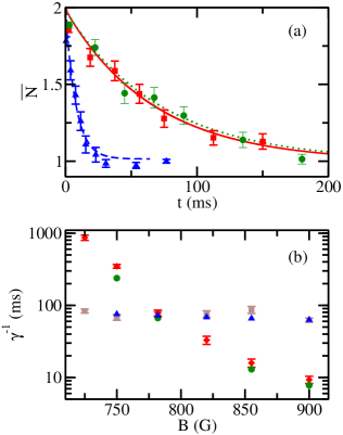
Figure 12: (Color online) Upper branch tunneling dynamics. (a) The dashed and solid lines show the mean number of trapped particles $\bar{N}$ obtained from our full time-dependent simulations as a function of time for two distinguishable particles at $B=900$G and $B=782$G, respectively, using the trap and interaction parameters given in Table 5. For comparison, triangles and squares with error bars show the corresponding experimental results footnote (11). The dotted line shows the mean number of trapped particles $\bar{N}$ obtained from our full time-dependent simulations as a function of time for two identical fermions at $B=782$G, using the trap parameters given in Table 6. For comparison, circles show the corresponding experimental results. (b) Circles and triangles show the time constant $\gamma^{-1}$ obtained from our full time-dependent simulations for two distinguishable particles and two identical fermions, respectively, as a function of the magnetic field strength $B$. For comparison, diamonds and squares with error bars show the corresponding experimental results footnote (11).

It is interesting to compare, as has been done in the experiments, the tunneling dynamics for two distinguishable particles with that for two identical particles, since two distinguishable but otherwise identical particles with infinitely large $g_{1\text{D}}$ are known to become fermionized Olshanii (1998); Girardeau and Olshanii (2003); Kanjilal and Blume (2004). In the present case, the distinguishable particles in states $|1\rangle$ and $|2\rangle$ feel slightly different trapping potentials. Thus the fermionization concept does, strictly speaking, not apply. However, since $\mathcal{C}_{|1\rangle}$ and $\mathcal{C}_{|2\rangle}$ at $B=782$G differ by only $0.2\%$, a meaningful comparison can be made. The dotted line in Fig. 12(a) shows the mean number of particles for two identical fermions in state $|2\rangle$. Since $\mathcal{C}_{|2\rangle}(782\text{G})<\mathcal{C}_{|1\rangle}$(782G), implying a higher barrier for the atom in state $|2\rangle$ than the atom in state $|1\rangle$, the non-interacting identical fermion system (two atoms in state $|2\rangle$) tunnels slightly slower than the two distinguishable atom system (one atom in state $|1\rangle$ and one atom in state $|2\rangle$) with infinitely large $g_{1\text{D}}$. Triangles and squares in Fig. 12(b) show the tunneling constants $\gamma^{-1}$ for two identical fermions as a function of $B$ obtained from our simulations (see Sec. IV.1 and Table 6) and from experiment, respectively. Although the fermionization is only approximate, Fig. 12(b) shows that the tunneling rate curves for two distinguishable particles and two identical non-interacting fermions cross at approximately $B=782$G, corresponding to $g_{1\text{D}}=\infty$ for the $|1\rangle$–$|2\rangle$ interaction.

Another consequence of the fact that $\mathcal{C}_{|2\rangle}(782\text{G})<\mathcal{C}_{|1\rangle}$(782G) is that the probability to find the particle ordering $z_{1}<z_{2}$ (or $z_{1}>z_{2}$) for two atoms in states $|1\rangle$ and $|2\rangle$ changes as a function of time. At $t=-t_{r}$, the probability $P_{z_{1}>z_{2}}$ to find $z_{1}>z_{2}$ is 0.525 and the probability $P_{z_{1}<z_{2}}$ to find $z_{1}<z_{2}$ is 0.475 [see Fig. 13(a)]. This is due to the fact that the particle in state $|1\rangle$ feels a “softer” confinement than the particle in state $|2\rangle$, i.e., $\omega_{\text{trap}}$ for state $|1\rangle$ is less than $\omega_{\text{trap}}$ for state $|2\rangle$. Importantly, the particles in states $|1\rangle$ and $|2\rangle$ at $B=782$G ($g_{\text{1D}}=\infty$) cannot pass through each other. Thus, since the particle in state $|1\rangle$ tunnels slightly faster than the particle in state $|2\rangle$ (see below) the probability $P_{z_{1}>z_{2}}$ to have $z_{1}>z_{2}$ inside the trap gets depleted faster than the probability to have $z_{1}<z_{2}$. Indeed, at $t=94$ms, we have $P_{z_{1}<z_{2}}=P_{z_{1}>z_{2}}$. At the end of the simulation ($t=350$ms), the probabilities to find an atom in state $|1\rangle$ and an atom in state $|2\rangle$ inside the trap are $48\%$ and $52\%$, respectively.

In the “ideal fermionization scenario”, in which the infinitely strongly interacting particles feel the same external potential, the ground state is two-fold degenerate. In our case, this degeneracy is broken since $\mathcal{C}_{|1\rangle}\neq\mathcal{C}_{|2\rangle}$. Solid and dotted lines in Fig. 13(a) show $|\Psi_{\text{rel}}(z_{12})|^{2}$,

$$\Psi_{\text{rel}}(z_{12})=\int_{-\infty}^{\infty}\Psi(z_{1},z_{2},t=-t_{r})dZ_{\text{CM}},$$ (18)

where $Z_{\text{CM}}=(z_{1}+z_{2})/2$, for the ground state and the first excited state, respectively. The difference of the amplitudes for $z_{12}<0$ and $z_{12}>0$ reflects the asymmetry of the trap potentials (see discussion above). The ground state wave function is greater or equal to zero everywhere while the first excited state wave function changes sign at $z_{12}=0$. The energy difference between the two states is approximately $3\times 10^{-4}E_{\text{ho}}$, corresponding to a time scale of 430ms.

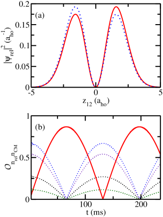
Figure 13: (Color online) Analysis of the upper branch time dynamics for two distinguishable particles interacting through a zero-range potential with $g_{1\text{D}}=\infty$ (the trap parameters are given in row 2 of Table 5). (a) The solid and dotted lines show the density $|\Psi_{\text{rel}}(z_{12})|^{2}$ of the lowest “eigenstate” and the first excited “eigenstate” at $t=-t_{r}$. These states are nearly degenerate. (b) The dotted lines show the normalized overlap $\mathcal{O}_{n_{\text{rel}}n_{\text{CM}}}$ between the wave packet $\Psi(z_{1},z_{2},t)$ and the harmonic oscillator states with even relative parity [from top to bottom, $(n_{\text{rel}},n_{\text{CM}})=$ (0,0), (2,0), (0,1), and (0,2)]. The solid line shows the overlap $\mathcal{O}_{n_{\text{rel}}n_{\text{CM}}}$ between the wave packet $\Psi(z_{1},z_{2},t)$ and the lowest harmonic oscillator state with odd relative parity, i.e., with $(n_{\text{rel}},n_{\text{CM}})=(1,0)$. The harmonic oscillator states are characterized by $a_{\text{trap}}=1.073a_{\text{ho}}$.

Since parity is not a conserved quantity and since the relative and center-of-mass degrees of freedom couple, we expect oscillations between the ground state and the first excited state at this time scale. Figure 13(b) shows the normalized overlap $\mathcal{O}_{n_{\text{rel}}n_{\text{CM}}}$,

$$\mathcal{O}_{n_{\text{rel}}n_{\text{CM}}}(t)=\left|\frac{\langle\Psi(z_{1},z_{2},t)|\phi_{n_{\text{rel}}n_{\text{CM}}}(z_{1},z_{2})\rangle}{\sqrt{\langle\Psi(z_{1},z_{2},t)|\Psi(z_{1},z_{2},t)\rangle}}\right|,$$ (19)

between the time-evolving wave packet $\Psi(z_{1},z_{2},t)$ and the two-body harmonic oscillator eigenstates $\phi_{n_{\text{rel}}n_{\text{CM}}}(z_{1},z_{2})$ with trap frequency $\omega_{\text{trap}}$ and relative and center-of-mass quantum numbers $n_{\text{rel}}$ and $n_{\text{CM}}$. The solid line shows the overlap for the anti-symmetric reference wave function $\phi_{n_{\text{rel}}n_{\text{CM}}}$ with $(n_{\text{rel}},n_{\text{CM}})=(1,0)$, which has odd relative parity. Dotted lines show the overlaps for states with even relative parity (see figure caption). The oscillation period, $T\approx 270$ms, is comparable to but smaller than the estimated value of 430ms because the system is modified after $t=-t_{r}$. Figure 13 demonstrates that two distinguishable particles with infinite $g_{1\text{D}}$ but $\mathcal{C}_{|1\rangle}\neq\mathcal{C}_{|2\rangle}$ exhibit unique dynamics that is absent for two identical fermions. It could be interesting in future work to tune the system toward and away from the ideal fermionization regime and to explore the resulting dynamics.

V Summary and outlook

This paper provided a detailed analysis of the two-particle tunneling dynamics out of an effectively one-dimensional trap. Our studies were motivated by experiments by the Heidelberg group and our analysis was based on full time-dependent simulations of single- and two-particle systems. We found that the trap calibration via a WKB analysis leads to an inaccurate trap parameterization; this finding is in agreement with a study by Lundmark et al. Lundmark et al. (2015). Using the reparameterized trapping potential, our tunneling rates for two identical fermions agree with the experimental results for all but two magnetic field strengths considered.

Our simulations for the interacting two-particle systems made a number of simplifying assumptions. The dynamics in the tight confinement direction was only incorporated indirectly via the renormalized one-dimensional coupling constant. For this, a harmonic trap in the tight direction was assumed. Moreover, we assumed simple short-range or zero-range interaction potentials. Deep-lying bound states and coupled channel effects were neglected entirely. Using the renormalized one-dimensional coupling constant $g_{1{\text{D}}}$ with the transverse frequency $\sqrt{p(0)}\omega_{\rho}^{\text{ref}}$ as input, our simulations reproduced the upper branch tunneling dynamics of the interacting two-particle system reasonably well. Our simulation results for the molecular branch dynamics agreed with the overall trend of the experiment but did not yield quantitative agreement. We argued that the actual transverse confinement felt by the atoms in the presence of the magnetic field gradient may be weaker than in the absence of the magnetic field gradient. This motivated us to calculate the one-dimensional coupling constant using a weaker transverse trapping frequency as input. The resulting two-particle tunneling rates are in agreement with the experimentally measured rates over the entire range of magnetic field strengths considered. We note that our finding is consistent with Ref. wall , which found that the non-separability of a gaussian trap affects the tunneling rate in a double-well geometry.

Our work suggests a number of follow-up studies. It would be interesting to extend the dynamical simulations to more particles and/or to include the tight confining directions. It would also be interesting to prepare other initial one- and two-particle states. For example, it would be interesting to investigate the tunneling dynamics from initial excited metastable states.

VI Acknowledgement

We thank S. Jochim and G. Zürn for clarifying various aspects of the experimental protocols and for stimulating discussions. We also thank P. Zhang for discussions, and Yangqian Yan and X. Y. Yin for generous help with parallelizing our time evolution code. Some of the calculations were performed on the WSU HPC. Support by the NSF through grant 1415112 is gratefully acknowledged.

Appendix A State dependence of the trapping potential and Breit-Rabi formula

We consider an atom with total (orbital and spin) electronic angular momentum quantum number $J=1/2$ and nuclear spin $I$ ($I=1$ for ⁶Li). In the absense of an external magnetic field, the energy difference $\Delta W$ between the hyperfine states $|F=I-1/2,m_{F}\rangle$ and $|F=I+1/2,m_{F}\rangle$ is independent of $m_{F}$. For ⁶Li with $|F=1/2\rangle$ and $|F=3/2\rangle$, $\Delta W$ is equal to $228.205$ MHz Metcalf and van der Straten (1999). According to the Breit-Rabi formula Breit and Rabi (1931); Ramsey (1985), the energy $W^{\text{BR}}_{|F,m_{F}\rangle}(B)$ of the hyperfine state $|F,m_{F}\rangle$ in an external magnetic field of strength $B$ is

$$W^{\text{BR}}_{|F,m_{F}\rangle}(B)=-\frac{\Delta W}{2(2I+1)}+g_{I}\mu_{B}m_{F}B$$

$$\pm\frac{\Delta W}{2}\left(1+\frac{4m_{F}}{2I+1}x+x^{2}\right)^{1/2},$$ (20)

where $x=(g_{J}-g_{I})\mu_{B}B/\Delta W$, $g_{J}$ is the Landé factor, and $g_{I}$ characterizes the magnetic moment of the nucleus. The plus and minus signs refer to states $F=I+1/2$ and $F=I-1/2$, respectively. The constants $g_{J}=2.0023019(24)$ and $g_{I}=-0.0004476493(45)$ are determined experimentally Böklen et al. (1967). Figure 1 shows the magnetic field dependence of the hyperfine states of ⁶Li for $F=1/2$ and $F=3/2$. The slope of these energy curves equals the negative of the magnetic moment of the atom Ramsey (1985), yielding

$$c_{|F,m_{F}\rangle}^{\text{BR}}(B)=-\frac{1}{\mu_{B}}\frac{d~{}}{dB}W^{\text{BR}}_{|F,m_{F}\rangle}(B).$$ (21)

Equation (21) characterizes the state and magnetic field dependence of the trapping potential (see Sec. II of the main text). The coefficients calculated according to Eqs. (20) and (21) are referred to as Breit-Rabi coefficients in the main text.

Appendix B Time dynamics for two identical fermions in an anti-symmetric state and in a product state

The wave packet of two identical fermions is anti-symmetric under the exchange of the particles. To calibrate the trap (see Sec. IV.1), the assumption in using the WKB approximation was that the dynamics could be described as if a single particle was tunneling out of the first excited trap state. Our numerical simulations show that the tunneling rates are, indeed, very similar. For the parameters listed in the third row of Table 6, we find $\gamma=13.8\text{s}^{-1}$ for the two-particle system and $\gamma_{\text{sp}}=13.5\text{s}^{-1}$ for the single-particle system. As we discuss now, the tunneling dynamics is, however, quite different.

Figure 14(a)

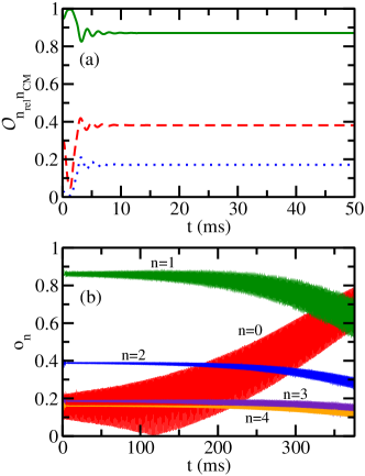
Figure 14: (Color online) (a) Analysis of the time dynamics for two identical fermions. The solid, dashed, and dotted lines show the normalized overlap $\mathcal{O}_{n_{\text{rel}}n_{\text{CM}}}$ between the wave packet $\Psi(z_{1},z_{2},t)$ and the harmonic oscillator states with odd relative parity [from top to bottom, $(n_{\text{rel}},n_{\text{CM}})=$ (1,0), (1,1), and (1,2)]. (b) Analysis of the time dynamics for a single atom in state $|2\rangle$, prepared in the first excited trap state at $t=-t_{r}$. The lines show the normalized overlaps $o_{n}(t)$ between the wave packet $\Psi(z,t)$ and the harmonic oscillator states with $n=0-4$. For both panels, the parameters $p(t=0)=0.68$, $z_{\text{R}}=8.548a_{\text{ho}}$, $c_{|2\rangle}^{\text{BR}}=0.99601$, and $B^{\prime}=1890$G/m are used.

shows the normalized overlaps $\mathcal{O}_{n_{\text{rel}}n_{\text{CM}}}$ [see Eq. (19)] between the time-evolving anti-symmetric two-particle wave packet $\Psi(z_{1},z_{2},t)$ and the two-body harmonic oscillator eigenstates $\phi_{n_{\text{rel}}n_{\text{CM}}}(z_{1},z_{2})$ with trap frequency $\omega_{\text{trap}}$ and relative and center-of-mass quantum numbers $n_{\text{rel}}$ and $n_{\text{CM}}$. The solid, dashed and dotted lines show the overlaps for $n_{\text{rel}}=1$ and $n_{\text{CM}}=0,1$, and $2$, respectively. The normalized overlaps oscillate for a short time ($t\lesssim 10$ms) and quickly approach constants. We see essentially constant overlaps till the end of our simulation at $t=500$ms. This indicates that the shape of the wave packet in region $R_{2}$ is constant in time. The overlaps vanish for even $n_{\text{rel}}$, indicating that the anti-symmetry of the wave packet is preserved during the time evolution.

Figure 14(b) shows the normalized overlap $o_{n}(t)$,

$$o_{n}(t)=\left|\frac{\langle\Psi(z,t)|\phi_{n}(z)\rangle}{\sqrt{\langle\Psi(z,t)|\Psi(z,t)\rangle}}\right|,$$ (22)

between the time-dependent single-particle wave packet $\Psi(z,t)$ and the time-independent single-particle harmonic oscillator functions $\phi_{n}(z)$ with quantum number $n$, $n=0-4$. The overlaps shown in Fig. 14(b) oscillate at a frequency that is close to the natural trap frequency $\omega_{\text{trap}}$ for $t>20$ms. Moreover, the “envelopes” of the overlaps change in time, indicating that the shape of the wave packet in region $R_{2}$ changes with time. At $t=0$, the wave packet has a finite overlap with the ground state harmonic oscillator wave function due to the change of the trapping potential. The contribution of the harmonic oscillator ground state to the wave packet is almost constant in time while the contributions of higher energy states deplete. This results in the increase of the normalized overlap $o_{0}(t)$ [see Fig. 14(b)]. In other words, as $P_{\text{sp,in}}(t)$ decreases, the wave packet looks more like the lowest-lying trap state as opposed to the initial state. As a consequence, the decay of $P_{\text{sp,in}}(t)$ with time deviates slightly from an exponential.

Appendix C Time propagation via Chebyshev expansion

The time evolution of the two-particle wave packet $\Psi(z_{1},z_{2},t)$ is given by

$$\Psi(z_{1},z_{2},t)=\mathcal{U}(t-t_{0})\Psi(z_{1},z_{2},t_{0}),$$ (23)

where the time-evolution operator $\mathcal{U}(t-t_{0})$ is

$$\mathcal{U}(t-t_{0})=\exp[-iH(t-t_{0})/\hbar].$$ (24)

To evaluate Eq. (23), one has to expand the time-evolution operator $\mathcal{U}(t-t_{0})$ in powers of $-iH(t-t_{0})/\hbar$. It has been shown that expanding $\mathcal{U}(t-t_{0})$ in terms of the complex Chebyshev polynomials $\phi_{k}$,

$$\mathcal{U}(t-t_{0})=\sum_{k=0}^{N}a_{k}\phi_{k}\left(\frac{-iH(t-t_{0})}{\hbar R}\right),$$ (25)

provides an efficient means to determine the time evolution of the wave packet Tal-Ezer and Kosloff (1984). Here, $R$ is a real and positive number that has been introduced to normalize the argument of $\phi_{k}$ such that $-iH(t-t_{0})/(\hbar R)\in[-i,i]$. A key point is that the recursion relation

$$\phi_{k}(X)=2X\phi_{k-1}(X)+\phi_{k-2}(X)$$ (26)

for the $k^{\text{th}}$ Chebyshev polynomial enables one to readily reach high orders in the expansion, allowing one to go to large $N$ in Eq. (25) and, correspondingly, to large $t-t_{0}$. The expansion coefficients $a_{k}$ are expressed in terms of Bessel functions of the first kind of order $k$. For more details, the reader is referred to Refs. Tal-Ezer and Kosloff (1984); Leforestier et al. (1991).

We use this approach to evaluate $\Psi(z_{1},z_{2},t)$ for $t>-t_{r}$. We choose time steps around $0.2\omega^{-1}$ and $N$ up to $800$. A time step of $0.2\omega^{-1}$ is small enough to resolve the tunneling dynamics and to extract the time dependence of the flux reliably, i.e., at the few percent accuracy level.

Appendix D Preparation of the initial state

In Secs. III and IV we need the initial (equilibrium) state of the trapped particles at $t=-t_{r}$. We use $p(t=-t_{r})=0.795$ for all cases. For this trap depth, tunneling is highly suppressed and the system is in a metastable state, i.e., it has a lifetime much larger than the time scale of the forthcoming tunneling process. To prepare the initial state, we “artificially” put a hard wall at $z=11a_{\text{ho}}$ (the top of the barrier is located at $z\approx 9a_{\text{ho}}$). We changed the position of the hard wall somewhat without seeing a notable change in the results. For example, for the upper branch calculations at $B=900$G, we changed the position of the hard wall to $10a_{\text{ho}}$ and $12a_{\text{ho}}$ and found that the overlap between the resulting initial states and the state prepared with the hardwall at $11a_{\text{ho}}$ deviated from 1 by less than $10^{-6}$. This artificial boundary condition leaves the trap in the “inside” region unchanged and completely turns off the tunneling. The resulting eigenstates are to a very good approximation equal to the metastable states of the trap with finite barrier.

We start with an initial wave packet that has a finite overlap with the state that we are looking for and act with the time-evolution operator, Eq. (24) with imaginary time $\tau$, on the initial wave packet Davies et al. (1980); Kosloff and Tal-Ezer (1986). To propagate the wave packet in imaginary time, we use the real time-propagation methods discussed in Appendices C and E with $t$ replaced by $\tau/i$. The initial wave packet can, in principle, be expanded in terms of unknown eigenfunctions of the Hamiltonian. After application of the time-evolution operator with imaginary time, each term in the expansion gets damped at a rate that is proportional to its energy. Thus, states with high energy decay fastest and eventually only the lowest energy state survives. We perform the imaginary time propagation using small $\Delta\tau$ and normalize the wave packet to one after each step. This process can be generalized to find excited states by removing the lower energy eigenstates from the Hilbert space Kosloff and Tal-Ezer (1986). In practice, this is done by orthogonalizing the evolving wave packet and the lower energy eigenstate(s) after each time step.

To implement the Chebychev expansion based approach with imaginary time, we expand the exponential function in terms of real Chebychev polynomials and use the corresponding recursion relation Kosloff and Tal-Ezer (1986). We typically use about 15 terms in the series and time steps around $(0.005\omega^{-1})/i$. The Trotter formula based propagation scheme with imaginary time does not involve integrals over highly oscillatory functions and the calculations are computationally much less expensive than those for the real time propagation.

Appendix E Time propagation for Hamiltonian with two-body zero-range interaction

The time propagation based on the Chebychev expansion is not applicable to the two-particle Hamiltonian with two-body zero-range interaction. In this case, we use a propagator that accounts for the two-body zero-range interaction exactly to determine the time evolution of the wave packet Blinder (1988); Wódkiewicz (1991). This propagator has recently been used in Monte Carlo simulations for systems with zero-range interactions Yan and Blume (2015). This appendix summarizes our implementation of the real time evolution in the presence of a zero-range two-body potential. The wave packet $\Psi$ at time $t+\Delta t$ can be written as

$$\Psi(z_{1},z_{2},t+\Delta t)=$$

$$\int_{-\infty}^{\infty}\int_{-\infty}^{\infty}\rho(z^{\prime}_{1},z^{\prime}_{2};z_{1},z_{2};\Delta t)\Psi(z^{\prime}_{1},z^{\prime}_{2},t)dz^{\prime}_{1}dz^{\prime}_{2},$$ (27)

where the zero-range propagator $\rho$ is defined through

$$\rho(z^{\prime}_{1},z^{\prime}_{2};z_{1},z_{2};\Delta t)=$$

$$\langle z^{\prime}_{1},z^{\prime}_{2}|\exp(-iH\Delta t/\hbar)|z_{1},z_{2}\rangle.$$ (28)

In free space, i.e., when the two-body Hamiltonian consists of the kinetic energy and the zero-range interaction, the propagator $\rho_{\text{free}}$ can be written as

$$\rho_{\text{free}}(z^{\prime}_{1},z^{\prime}_{2};z_{1},z_{2};\Delta t)=\rho_{\text{free}}^{\text{sp}}(z^{\prime}_{1},z_{1},\Delta t)$$

$$\times\rho_{\text{free}}^{\text{sp}}(z^{\prime}_{2},z_{2},\Delta t)\rho_{\text{free}}^{\text{rel}}(z_{1}^{\prime}-z^{\prime}_{2},z_{1}-z_{2},\Delta t),$$ (29)

where $\rho_{\text{free}}^{\text{sp}}$,

$$\rho_{\text{free}}^{\text{sp}}(z^{\prime},z,\Delta t)=$$

$$\left(\frac{m}{2\pi i\Delta t\hbar}\right)^{1/2}\exp\left(-\frac{m(z-z^{\prime})^{2}}{2i\Delta t\hbar}\right),$$ (30)

accounts for the single-particle kinetic energy and $\rho_{\text{free}}^{\text{rel}}$,

$$\rho_{\text{free}}^{\text{rel}}(z^{\prime},z,\Delta t)=1-\exp\left(-\frac{m(zz^{\prime}+|zz^{\prime}|)}{2i\Delta t\hbar}\right)$$

$$\times\sqrt{\frac{mi\pi\Delta t}{4\hbar}}\frac{g_{1\text{D}}}{\hbar}\exp\left(u^{2}\right)\text{erfc}(u),$$ (31)

for the two-body zero-range potential Blinder (1988); Wódkiewicz (1991). In Eq. (31), erfc denotes the complementary error function and $u$ is equal to $m(|z|+|z^{\prime}|+ig_{1\text{D}}\Delta t/\hbar)/\sqrt{4mi\Delta t\hbar}$. For infinitely strong interaction, i.e., for $|g_{1\text{D}}|=\infty$, Eq. (31) simplifies to

$$\rho_{\text{free}}^{\text{rel}}(z^{\prime},z,\Delta t)=\left\{\begin{array}[]{l r}1-\exp\left(-\frac{mzz^{\prime}}{i\Delta t\hbar}\right)&\text{for}\quad zz^{\prime}>0\\ 0&\text{for}\quad zz^{\prime}\leq 0\end{array}\right..$$

In the presence of the external potential $V_{\text{ext}}$, we use the Trotter formula Trotter (1959),

$$\rho(z^{\prime}_{1},z^{\prime}_{2};z_{1},z_{2};\Delta t)\approx\exp\left(-\frac{i\Delta t}{2\hbar}V_{\text{ext}}(z_{1}^{\prime},z_{2}^{\prime})\right)$$

$$\times\rho_{\text{free}}(z^{\prime}_{1},z^{\prime}_{2};z_{1},z_{2};\Delta t)\exp\left(-\frac{i\Delta t}{2\hbar}V_{\text{ext}}(z_{1},z_{2})\right).$$ (32)

This decomposition yields an error in the propagator that is proportional to $\Delta t^{3}$. We use Eq. (27) with $\rho$ given by Eq. (32) to propagate the wave packet in real time for each time step $\Delta t$. Unlike the Chebychev expansion approach, the Trotter formula based approach is limited to small $\Delta t$. Importantly, the integrand in Eq. (27) oscillates with a frequency that is proportional to $1/\Delta t$. To resolve these oscillations we need to choose a sufficiently dense spatial grid for the numerical integration of the right hand side of Eq. (27). We typically use a grid spacing $\Delta z_{j}/a_{\text{ho}}\leq\Delta t/(10\omega^{-1})$ ($j=1$ and 2). We find that a value of $\Delta t\leq 0.2\omega^{-1}$ ensures that the norm of the wave packet, accounting for the absorbed portion of the wave packet, is 0.99 (or even closer to one) at the end of our simulation. Due to the need to evaluate the two-dimensional integral for each grid point, the Trotter formula based propagation scheme is much more computationally demanding than the Chebychev polynomial based propagation scheme.

Appendix F Application of the absorbing potential

The damping of the wave packet in the numerical regions $R_{1An}$, $R_{0n}$, and $R_{1Bn}$ has the same effect as an absorbing potential. After each time step, we multiply the wave packet by $\mathcal{D}(z_{1})\mathcal{D}(z_{2})$ Sun et al. (2009), where

$$\mathcal{D}(z)=\left\{\begin{array}[]{l l}1&\text{for}\quad z<z_{d}\\ \exp{\left[-\alpha\left(\frac{z-z_{d}}{\Delta_{d}}\right)^{n_{d}}\right]}&\text{for}\quad z\geq z_{d}\end{array}\right..$$

Here, $\Delta_{d}$, $\alpha$, and $n_{d}$ are parameters whose values depend, in general, on the kinetic energy of the particle that is being absorbed. We use $\Delta_{d}=10a_{\text{ho}}$, $\alpha=5$, and $n_{d}=2$ with $z_{hw}-z_{d}\geq 6a_{\text{ho}}$, where $z_{hw}$ is the position of the hard wall at the end of the simulation grid. This parameter combination ensures that the reflection from the end of the numerical box is negligibly small.

Appendix G Flux analysis

In this Appendix we discuss how to extract physical quantities from the density flux. $P_{n}(t)$ denotes the probability to find $n$ particles ($n=0,1,$ or 2) inside the trap at time $t$. $P_{2}(t)$ is obtained by integrating the density $|\Psi(z_{1},z_{2},t)|^{2}$ over the region $R_{2}$ (see Fig. 5),

$$P_{2}(t)=\int_{R_{2}}|\Psi(z_{1},z_{2},t)|^{2}dz_{1}dz_{2}.$$ (33)

The initial condition is given by $P_{2}(-t_{r})=1$, i.e., at time $t=-t_{r}$ both particles are inside the trap. For $t>-t_{r}$, we have $P_{2}(t)+P_{1}(t)+P_{0}(t)=1$. The density $|\Psi(z_{1},z_{2},t)|^{2}$ can flow from one region to another during the time propagation. To quantify the change of $P_{n}(t)$, we use the current ${\bf{j}}(z_{1},z_{2},t)$,

$${\bf{j}}(z_{1},z_{2},t)=-\frac{\hbar}{m}\text{Im}\left[\Psi^{*}(z_{1},z_{2},t)\;{\boldsymbol{\nabla}}\Psi(z_{1},z_{2},t)\right],$$ (34)

where

$${\boldsymbol{\nabla}}=\frac{\partial}{\partial z_{1}}{\bf{\hat{z}}}_{1}+\frac{\partial}{\partial z_{2}}{\bf{\hat{z}}}_{2}.$$ (35)

Here, ${\bf{\hat{z}}}_{1}$ and ${\bf{\hat{z}}}_{2}$ are the unit vectors in the $z_{1}$ and $z_{2}$ directions, respectively. At each point in time and space, the continuity equation requires

$$\frac{\partial|\Psi(z_{1},z_{2},t)|^{2}}{\partial t}+{\boldsymbol{\nabla}}\cdot{\bf{j}}(z_{1},z_{2},t)=0.$$ (36)

If we integrate Eq. (36) over the region $R_{i}$ ($R_{i}$ can be equal to $R_{2}$, $R_{1A}$, or $R_{1B}$; see Fig. 5), we find

$$\frac{\partial}{\partial t}\int_{R_{i}}|\Psi(z_{1},z_{2},t)|^{2}\;dz_{1}dz_{2}=$$

$$-\int_{R_{i}}{\boldsymbol{\nabla}}\cdot{\bf{j}}(z_{1},z_{2},t)\;dz_{1}dz_{2}.$$ (37)

The left hand side of Eq. (37) is the rate at which the probability of finding the system in region $R_{i}$ changes. To simplify the right hand side, we use the divergence theorem in two spatial dimensions,

$$\int_{R_{i}}{\boldsymbol{\nabla}}\cdot{\bf{j}}(z_{1},z_{2},t)\;dz_{1}dz_{2}=$$

$$\oint_{B_{i}}{\bf{j}}(z_{1},z_{2},t)\cdot{\bf{\hat{n}}}_{i}\;dl.$$ (38)

Here, $dl$ is the line element corresponding to the closed boundary $B_{i}$ that encircles region $R_{i}$ and ${\bf{\hat{n}}}_{i}$ is the unit vector perpendicular to the boundary and directed out of the region $R_{i}$. Equation (37) can thus be written as

$$\frac{\partial}{\partial t}\int_{R_{i}}|\Psi(z_{1},z_{2},t)|^{2}\;dz_{1}dz_{2}=$$

$$-\oint_{B_{i}}{\bf{j}}(z_{1},z_{2},t)\cdot{\bf{\hat{n}}}_{i}\;dl.$$ (39)

The change of the probability to find the system in region $R_{i}$ can be obtained from the flux through the boundary $B_{i}$. Applying Eq. (39) to region $R_{2}$, we obtain

$$\frac{\partial P_{2}(t)}{\partial t}=-\oint_{B_{2}}{\bf{j}}(z_{1},z_{2},t)\cdot{\bf{\hat{n}}}_{2}\;dl$$ (40)

or

$$P_{2}(t)=1-\int_{-t_{r}}^{t}\oint_{B_{2}}{\bf{j}}(z_{1},z_{2},t)\cdot{\bf{\hat{n}}}_{2}\;dl\;dt.$$ (41)

To extract additional information from Eq. (39), we break the boundary $B_{2}$ into pieces. In particular, flux through the boundary $b_{2,0}$ corresponds to the correlated tunneling of two particles (pair tunneling) and flux through the boundaries $b_{2,1A}$ and $b_{2,1B}$ corresponds to single-particle tunneling (one particle tunnels and one remains in the trap). To quantify this in terms of tunneling rates, we define the rate $\gamma_{2}$ at which $P_{2}(t)$ decays during the time $\Delta t$ through

$$\gamma_{2}=-\frac{1}{P_{2}(t)}\frac{\Delta P_{2}(t)}{\Delta t}.$$ (42)

Next, we divide the quantity $\Delta P_{2}(t)$ into two pieces, namely the change $\Delta P_{2\to 0}(t)$ due to the pair tunneling (flux through the boundary $b_{2,0}$) and the change $\Delta P_{2\to 1}(t)$ due to the single-particle tunneling (flux through the boundaries $b_{2,1A}$ and $b_{2,1B}$),

$$\Delta P_{2}(t)=\Delta P_{2\to 0}(t)+\Delta P_{2\to 1}(t).$$ (43)

Defining the pair tunneling rate $\gamma_{\text{P}}$ and the single-particle tunneling rate $\gamma_{\text{s}}$,

$$\gamma_{\text{P}}=-\frac{1}{P_{2}(t)}\frac{\Delta P_{2\to 0}(t)}{\Delta t}$$ (44)

and

$$\gamma_{\text{s}}=-\frac{1}{P_{2}(t)}\frac{\Delta P_{2\to 1}(t)}{\Delta t},$$ (45)

we have $\gamma_{2}=\gamma_{\text{P}}+\gamma_{\text{s}}$. $\gamma_{\text{P}}$ and $\gamma_{\text{s}}$ oscillate in time for $t$ not much larger than $t_{r}$ (typically $t\lesssim 20$ms) and are essentially constant for large $t$ ($t\gtrsim 20$ms). The values reported in the main text are obtained by fitting the numerical data for sufficiently large $t$.

If $z_{\text{d}}\to\infty$, we can find $P_{1}(t)$ by integrating the density $|\Psi(z_{1},z_{2},t)|^{2}$ over the regions $R_{1A}$ and $R_{1B}$ (see Fig. 5) or, equivalently, by analyzing the flux through boundaries $b_{2,1A}$, $b_{1A,0}$, $b_{2,1B}$, and $b_{1B,0}$. The average direction of the flux is into the region $R_{1A}$ ($R_{1B}$) through boundary $b_{2,1A}$ ($b_{2,1B}$) and out of the region $R_{1A}$ ($R_{1B}$) through boundary $b_{1A,0}$ ($b_{1B,0}$). In the upper branch simulations, we find vanishing flux through boundaries $b_{1A,0}$ and $b_{1B,0}$. Thus, without worrying about the finite size of the simulation box, we can determine $P_{1}(t)$ as the sum of the fluxes through boundaries $b_{2,1A}$ and $b_{2,1B}$,

$$P_{1}(t)=-\int_{-t_{r}}^{t}\bigg{\{}\int_{b_{2,1A}}{\bf{j}}(z_{1},z_{2},t)\cdot{\bf{\hat{n}}}_{1A}\;dl~{}~{}~{}~{}~{}$$

$$+\int_{b_{2,1B}}{\bf{j}}(z_{1},z_{2},t)\cdot{\bf{\hat{n}}}_{1B}\;dl\bigg{\}}dt.$$ (46)

It should be noted that if the flux through boundaries $b_{1A,0}$ and $b_{1B,0}$ is non-zero, then the evaluation of $P_{1}(t)$ is more involved; this case is not discussed here.

Appendix H Additional comments on the WKB approximation

As discussed in the main text, the WKB approximation yields single-particle tunneling rates that are smaller (larger) than the exact tunneling rates for the trap ground state (first excited trap state). To elaborate on this behavior, we determine $p(t=0)$ for the trap ground state, the first excited trap state, and the second excited trap state such that (a) ${\mathcal{T}}=0.06267$ and (b) ${\mathcal{T}}=0.0063$. We then perform exact single-particle time propagation calculations for these cases, starting with a quasi-eigenstate (either the ground state, the first excited trap state, or the second excited trap state) for $p(t=-t_{r})=0.795$. Table 7 summarizes the resulting tunneling rates $\gamma_{\text{sp}}^{\text{num}}$. It can be seen that $\gamma_{\text{sp}}^{\text{num}}$ is approximately independent of the state number but, as expected, strongly dependent on the actual barrier the particle has to tunnel through.

Table 7: Single-particle WKB versus exact tunneling rates. The tunneling coefficients for cases (a) and (b) are $\mathcal{T}=0.06267$ and $\mathcal{T}=0.0063$, respectively. The third column reports the value of $p(t=0)$ for which the trap ground state, first excited trap state, and second excited trap state yield the desired $\mathcal{T}$. The fourth and fifth columns report the WKB frequency $f^{\text{WKB}}$ and the single particle WKB tunneling rate $\gamma_{\text{sp}}^{\text{WKB}}$, Eq. (6), respectively. For comparison, the sixth column reports the tunneling rate $\gamma_{\text{sp}}^{\text{num}}$ obtained from our exact time-dependent simulations. The calculations are performed for $\mathcal{C}=1890$G/m, $V_{0}=56.16E_{\text{ho}}$, and $z_{\text{R}}=8.548a_{\text{ho}}$.

case	trap state	$p(t=0)$	$f^{\text{WKB}}$ ($\text{ms}^{-1}$)	$\gamma^{\text{WKB}}_{\text{sp}}$ ($\text{ms}^{-1}$)	$\gamma^{\text{num}}_{\text{sp}}$ ($\text{ms}^{-1}$)
(a)	gr. st	0.63540	0.322	0.0202	0.0330
(a)	1st exc. st.	0.67687	1.104	0.0692	0.0330
(a)	2nd exc. st.	0.71486	1.999	0.1253	0.0329
(b)	gr. st	0.6489	0.352	0.00222	0.00406
(b)	1st exc. st.	0.6899	1.1732	0.00739	0.00403
(b)	2nd exc. st.	0.7277	2.0965	0.013215	0.00400

Due to the dependence of $f^{\text{WKB}}$ on the state (through the WKB energy), the WKB rates $\gamma_{\text{sp}}^{\text{WKB}}$ for the three states vary by about a factor of 6 for cases (a) and (b). For the parameters considered in Table 7 and in the main text, the WKB rate for the ground state is smaller than that obtained through the full time propagation, with the ratio $\gamma_{\text{sp}}^{\text{WKB}}/\gamma_{\text{sp}}^{\text{num}}$ depending on the exact shape of the trap. For the excited states, in contrast, the WKB rates are larger than those obtained through the full time propagation.

References

- Breuer and Petruccione (2007) H. P. Breuer and F. Petruccione, The Theory of Open Quantum Systems (OUP Oxford, 2007).
- Wiseman and Milburn (2010) H. M. Wiseman and G. J. Milburn, Quantum Measurement and Control (Cambridge University Press, 2010).
- Bloch et al. (2008) I. Bloch, J. Dalibard, and W. Zwerger, “Many-body physics with ultracold gases,” Rev. Mod. Phys. 80, 885–964 (2008).
- Blume (2012) D. Blume, “Few-body physics with ultracold atomic and molecular systems in traps,” Reports on Progress in Physics 75, 046401 (2012).
- Giorgini et al. (2008) S. Giorgini, L. P. Pitaevskii, and S. Stringari, “Theory of ultracold atomic Fermi gases,” Rev. Mod. Phys. 80, 1215–1274 (2008).
- Chin et al. (2010) C. Chin, R. Grimm, P. Julienne, and E. Tiesinga, “Feshbach resonances in ultracold gases,” Rev. Mod. Phys. 82, 1225–1286 (2010).
- Langen et al. (2015) T. Langen, S. Erne, R. Geiger, B. Rauer, T. Schweigler, M. Kuhnert, W. Rohringer, I. E. Mazets, T. Gasenzer, and J. Schmiedmayer, “Experimental observation of a generalized Gibbs ensemble,” Science 348, 207–211 (2015).
- Yan et al. (2013) B. Yan, S. A. Moses, B. Gadway, J. P. Covey, K. R. A. Hazzard, A. M. Rey, D. S. Jin, and J. Ye, “Observation of dipolar spin-exchange interactions with lattice-confined polar molecules,” Nature 501, 521–525 (2013).
- Zürn et al. (2012) G. Zürn, F. Serwane, T. Lompe, A. N. Wenz, M. G. Ries, J. E. Bohn, and S. Jochim, “Fermionization of two distinguishable fermions,” Phys. Rev. Lett. 108, 075303 (2012).
- Zürn et al. (2013a) G. Zürn, A. N. Wenz, S. Murmann, A. Bergschneider, T. Lompe, and S. Jochim, “Pairing in few-fermion systems with attractive interactions,” Phys. Rev. Lett. 111, 175302 (2013a).
- Razavy (2013) M. Razavy, Quantum Theory of Tunneling (World Scientific Publishing Company Pte Limited, 2013).
- Oka et al. (2014) H. Oka, O. O. Brovko, M. Corbetta, V. S. Stepanyuk, D. Sander, and J. Kirschner, “Spin-polarized quantum confinement in nanostructures: Scanning tunneling microscopy,” Rev. Mod. Phys. 86, 1127–1168 (2014).
- Serway et al. (2004) R. Serway, C. Moses, and C. Moyer, Modern Physics (Cengage Learning, 2004).
- Eckle et al. (2008) P. Eckle, A. N. Pfeiffer, C. Cirelli, A. Staudte, R. Dörner, H. G. Muller, M. Büttiker, and U. Keller, “Attosecond ionization and tunneling delay time measurements in helium,” Science 322, 1525–1529 (2008).
- Lode et al. (2012) A. U. J. Lode, A. I. Streltsov, K. Sakmann, O. E. Alon, and L. S. Cederbaum, “How an interacting many-body system tunnels through a potential barrier to open space,” Proceedings of the National Academy of Sciences 109, 13521–13525 (2012).
- Hunn et al. (2013) S. Hunn, K. Zimmermann, M. Hiller, and A. Buchleitner, “Tunneling decay of two interacting bosons in an asymmetric double-well potential: A spectral approach,” Phys. Rev. A 87, 043626 (2013).
- Kim and Brand (2011) S. Kim and J. Brand, “Decay modes of two repulsively interacting bosons,” Journal of Physics B: Atomic, Molecular and Optical Physics 44, 195301 (2011).
- Lode et al. (2009) A. U. J. Lode, A. I. Streltsov, O. E. Alon, H.-D. Meyer, and L. S. Cederbaum, “Exact decay and tunnelling dynamics of interacting few-boson systems,” Journal of Physics B: Atomic, Molecular and Optical Physics 42, 044018 (2009).
- Rontani (2012) M. Rontani, “Tunneling theory of two interacting atoms in a trap,” Phys. Rev. Lett. 108, 115302 (2012).
- Rontani (2013) M. Rontani, “Pair tunneling of two atoms out of a trap,” Phys. Rev. A 88, 043633 (2013).
- Lundmark et al. (2015) R. Lundmark, C. Forssén, and J. Rotureau, “Tunneling theory for tunable open quantum systems of ultracold atoms in one-dimensional traps,” Phys. Rev. A 91, 041601(R) (2015).
- Ankerhold (2007) J. Ankerhold, Quantum Tunneling in Complex Systems: The Semiclassical Approach, (Springer, 2007).
- Breit and Rabi (1931) G. Breit and I. I. Rabi, “Measurement of nuclear spin,” Phys. Rev. 38, 2082–2083 (1931).
- Zur (May 7, 2015) G. Zürn, private communication (May 7, 2015).
- (25) The rate reported in the supplementary material of Ref. Zürn et al. (2012) is an average over 9 measurements for magnetic field strengths between G and G [G. Zürn, private communication (July 24, 2015)].
- Zürn et al. (2013b) G. Zürn, T. Lompe, A. N. Wenz, S. Jochim, P. S. Julienne, and J. M. Hutson, “Precise characterization of feshbach resonances using trap-sideband-resolved rf spectroscopy of weakly bound molecules,” Phys. Rev. Lett. 110, 135301 (2013b).
- Olshanii (1998) M. Olshanii, “Atomic scattering in the presence of an external confinement and a gas of impenetrable bosons,” Phys. Rev. Lett. 81, 938–941 (1998).
- Sala et al. (2013) S. Sala, G. Zürn, T. Lompe, A. N. Wenz, S. Murmann, F. Serwane, S. Jochim, and A. Saenz, “Coherent molecule formation in anharmonic potentials near confinement-induced resonances,” Phys. Rev. Lett. 110, 203202 (2013).
- Peng et al. (2011) S.-G. Peng, H. Hu, X.-J. Liu, and P. D. Drummond, “Confinement-induced resonances in anharmonic waveguides,” Phys. Rev. A 84, 043619 (2011).
- Peano et al. (2005) V. Peano, M. Thorwart, C. Mora, and R. Egger, “Confinement-induced resonances for a two-component ultracold atom gas in arbitrary quasi-one-dimensional traps,” New Journal of Physics 7, 192 (2005).
- Melezhik and Schmelcher (2009) V. S. Melezhik and P. Schmelcher, “Quantum dynamics of resonant molecule formation in waveguides,” New Journal of Physics 11, 073031 (2009).
- Gharashi et al. (2014) S. E. Gharashi, X. Y. Yin, and D. Blume, “Molecular branch of a small highly elongated Fermi gas with an impurity: Full three-dimensional versus effective one-dimensional description,” Phys. Rev. A 89, 023603 (2014).
- footnote (6) The size of the free-space molecule for the zero-range interaction is equal to but for the finite-range interaction corrections must be applied.
- footnote (5) The experimental data for the interacting systems are taken from Table II of Ref. Zürn et al. (2013a) and the experimental data point for the non-interacting system is obtained by adding the measured single-particle tunneling rates reported in Table I of Ref. Zürn et al. (2013a).
- footnote (11) The experimental data shown in Fig. 12 and Tables 5 and 6 were kindly provided to us in tabular form by G. Zürn [private communication (May 6, 2015)]. These data are shown in Figs. 3 and 4(a) of Ref. Zürn et al. (2012). G. Zürn pointed out that the magnetic fields reported in Ref. Zürn et al. (2012) are about 1G too low. The recalibrated magnetic field values lead to small changes of and thus . Our simulations, however, use the magnetic field values reported in Ref. Zürn et al. (2012). We estimate that the use of the recalibrated magnetic field values would increase the two-particle values of by around for G.
- Girardeau and Olshanii (2003) M. D. Girardeau and M. Olshanii, “Fermi-Bose mapping and N-particle ground state of spin-polarized fermions in tight atom waveguides,” eprint arXiv:cond-mat/0309396 (2003).
- Kanjilal and Blume (2004) K. Kanjilal and D. Blume, “Nondivergent pseudopotential treatment of spin-polarized fermions under one- and three-dimensional harmonic confinement,” Phys. Rev. A 70, 042709 (2004).
- (38) M. L. Wall, K. R. A. Hazzard, and A. M. Rey, ”Effective many-body parameters for atoms in nonseparable Gaussian optical potentials,” Phys. Rev. A 92, 013610 (2015).
- Metcalf and van der Straten (1999) H. J. Metcalf and P. van der Straten, Laser Cooling and Trapping, Graduate Texts in Contemporary Physics (Springer New York, 1999).
- Ramsey (1985) N. Ramsey, Molecular Beams, International series of monographs on Physics (OUP Oxford, 1985).
- Böklen et al. (1967) K. D. Böklen, W. Dankwort, E. Pitz, and S. Penselin, “High precision measurements of the -factors of the alkalis using the atomic beam magnetic resonance method,” Zeitschrift für Physik 200, 467–486 (1967).
- Tal-Ezer and Kosloff (1984) H. Tal-Ezer and R. Kosloff, “An accurate and efficient scheme for propagating the time dependent Schrödinger equation,” The Journal of Chemical Physics 81, 3967–3971 (1984).
- Leforestier et al. (1991) C. Leforestier, R. H. Bisseling, C. Cerjan, M. D. Feit, R. Friesner, A. Guldberg, A. Hammerich, G. Jolicard, W. Karrlein, H.-D. Meyer, N. Lipkin, O. Roncero, and R. Kosloff, “A comparison of different propagation schemes for the time dependent Schrödinger equation,” Journal of Computational Physics 94, 59 – 80 (1991).
- Davies et al. (1980) K. T. R. Davies, H. Flocard, S. Krieger, and M. S. Weiss, “Application of the imaginary time step method to the solution of the static Hartree-Fock problem,” Nuclear Physics A 342, 111–123 (1980).
- Kosloff and Tal-Ezer (1986) R. Kosloff and H. Tal-Ezer, “A direct relaxation method for calculating eigenfunctions and eigenvalues of the Schrödinger equation on a grid,” Chemical Physics Letters 127, 223 – 230 (1986).
- Blinder (1988) S. M. Blinder, “Green’s function and propagator for the one-dimensional -function potential,” Phys. Rev. A 37, 973–976 (1988).
- Wódkiewicz (1991) K. Wódkiewicz, “Fermi pseudopotential in arbitrary dimensions,” Phys. Rev. A 43, 68–76 (1991).
- Yan and Blume (2015) Y. Yan and D. Blume, “Incorporating exact two-body propagators for zero-range interactions into -body Monte Carlo simulations,” Phys. Rev. A 91, 043607 (2015).
- Trotter (1959) H. F. Trotter, “On the product of semi-groups of operators,” Proc. Amer. Math. Soc. 10, 545–551 (1959).
- Sun et al. (2009) Z. Sun, S.-Y. Lee, H. Guo, and D. H. Zhang, “Comparison of second-order split operator and Chebyshev propagator in wave packet based state-to-state reactive scattering calculations,” The Journal of Chemical Physics 130, 174102 (2009).