Relativistic few-body methods

W. N. Polyzou
Department of Physics and Astronomy
The University of Iowa
Iowa City, IA 52242, USA

Contribution to the 21-st International Conference on Few-Body Problems in Physics

• I discuss the role of relativistic quantum mechanics in few-body physics, various formulations of relativistic few-body quantum mechanics and how they are related.

1 Introduction

The observable degrees of freedom in any experiment are particles. Particles appear as initial and final states in scattering experiments. They are also the elementary building blocks of complex systems from nuclei to stars. While interactions do not conserve particle number, if the $S$-matrix is unitary then all of the reaction products remain particles. This observation implies that it must be possible to reformulate mathematical models of any physical system directly in terms of particle degrees of freedom. Since relativistic invariance is a fundamental symmetry of physical systems, it follows that it must be possible to represent mathematical models of physical systems as relativistically invariant quantum theories of particles.

If the underlying theory is a quantum field theory that describes interacting particles, it must have a representation as a relativistically invariant quantum theory of particles. The most interesting case is QCD, where the field theory involves non-observable quark and gluon degrees of freedom, but the theory ultimately describes reactions where the observable initial and final states are baryons and mesons. When expressed in terms of mesons and baryon degrees of freedom, QCD has the structure of a relativistic quantum theory of interacting particles. In the particle representation the degrees of freedom are experimentally observable, but the interactions necessarily become complicated. One important challenge is to construct the interactions between particles directly from QCD. If these interactions could be determined, it is likely that the particle representation of QCD would be a more efficient representation for calculating scattering observables, since the particle degrees of freedom are directly related to experiment. For this reason it also makes sense model these interactions by combining fundamental principles with experimental constraints.

The general principles of relativistic quantum theory provide representation independent constraints on these interactions. These constraints are non-trivial and may not be compatible with some truncations of the field theory. In addition, these constraints provide guidance in constructing realistic models of few hadron systems that remain valid at relativistic energies.

I discuss various representation of relativistic quantum theories of particles and their relation to each other and to different representations of quantum field theory. One of the challenges of this subject is that there are may different representations. Some are more suited to computation while others are more directly related to an underlying quantum field theory. The equivalence between different representations is an important tool for understanding the structure of realistic models.

2 Relativistic invariance - general considerations

Relativistic invariance is a symmetry of quantum theory which requires that quantum probabilities for equivalent experiments performed in different inertial frames are identical. Mathematically this requires that there is a unitary representation of the Poincaré group [1] $U(\Lambda,a)$

$$U(\Lambda_{2},a_{2})U(\Lambda_{1},a_{1})=U(\Lambda_{2}\Lambda_{1},\Lambda_{2}a_{1}+a_{2})$$ (1)

(the semidirect product of the Lorentz group with the spacetime translation group) on the Hilbert space of the quantum theory. Here $\Lambda$ is a Lorentz transformation connected to the identity and $a$ is a space-time translation parameter.

In addition, the ability to test special relativity by performing measurements on isolated subsystems requires that the unitary representation of the Poincaré group asymptotically approaches a tensor product of subsystem representations when the subsystems are asymptotically separated:

$$\lim_{|r_{i}-r_{j}|\to\infty}U(\Lambda,a)=U_{i}(\Lambda,a)\otimes U_{j}(\Lambda,a).$$ (2)

The smallest of these isolated subsystems are single-particle subsystems, which are the building blocks of the particle representation. The constraints (2) are fundamental constraints on acceptable models or truncations of field theories to a computable number of degrees of freedom.

3 Hilbert space representations

While there are many ways to construct unitary representations of the Poincaré group, the common feature of all of these representations is that they can always be decomposed into direct integrals of irreducible representations. This decomposition is the relativistic analog of diagonalizing the Hamiltonian in non-relativistic quantum mechanics. The diagonalization is more complicated in the relativistic case because it is necessary to simultaneously diagonalize the mass and spin Casimir operators. Both of these operators involve interactions in relativistic theories that satisfy (2).

The structure of the physical Hilbert space has a significant effect on the structure of the dynamical unitary representation of the Poincaré group. Covariant representations, which are typical of field theories, have Hilbert space inner products with non-trivial kernels, where the dynamics is encoded in the kernel. In explicit particle representations the dynamics appears in the unitary representation of the Poincaré group. The three most common representation are discussed below.

• Local field theory. In this representation vacuum expectation values of products of fields appear in the kernel the Hilbert space scalar product:

  $$W_{n}(x)=W_{n}(x_{1},\cdots,x_{n}):=\langle 0|\phi(x_{1})\cdots\phi(x_{n})|0\rangle$$ (3)

  $$\langle f|g\rangle=\sum_{mn}\int f^{*}_{m}(x)W_{m+n}(x,y)g_{n}(y)d^{4m}xd^{4n}y.$$ (4)

• Euclidean field theory. In this representation the Euclidean Green functions,

  $$S_{n}(x)=S_{n}(x_{1}\cdots x_{n})=\int D[\phi]d^{-A[\phi]}\phi(x_{1})\cdots\phi(x_{n}),$$ (5)

  which are formally moments of a Euclidean path integral, appear in the kernel of the physical Hilbert space inner product [2]

  $$\langle f|g\rangle=\sum_{mn}\int f^{*}_{m}(Rx)S_{m+n}(x;y)g_{n}(y)d^{4m}xd^{4n}y$$ (6)

  where $R$ is the Euclidean time reversal operator and the test functions $f$ have support for positive relative Euclidean times. The collection of Euclidean Green functions $\{S_{n}\}$ are called reflection positive if $\|f\|=\langle f|f\rangle$ above is non-negative.

• Direct interaction representations. The Hilbert space is the direct sum of tensor products of mass $m$ spin $j$ irreducible representation spaces ${\cal H}_{mj}$:

  $${\cal H}=\oplus(\otimes{\cal H}_{mj}).$$ (7)

  This is the Hilbert space for a collection of free relativistic particles. Explicit dynamical representations of the Poincaré group or Lie algebra are constructed on this space.

• Schwinger-Dyson - quasipotential representations. In this representation the dynamical quantities are time-ordered Green functions

  $$G_{n}(x_{1},\cdots,x_{n})=\langle 0|T(\phi(x_{1})\cdots\phi(x_{n}))|0\rangle$$ (8)

• where $T$ is the time ordering operator.

• While these functions do not have a direct relation to a Hilbert space inner product, they can be used to calculate matrix elements of any operator between physical particle states [3]. In principle both the time-ordered Green functions, $G_{n}$, and the Wightman functions, $W_{n}$, are related to the Euclidean Green functions, $S_{n}$, by different analytic continuations. It follows that both have the same dynamical content.

• Quasipotential methods replace the equations for the time-ordered Green functions by equivalent equations for quasipotentials and constrained time ordered Green functions. The simplest example is the Schwinger-Dyson equation for the four point function, $G_{4}$, which is the Bethe-Salpeter equation:

  $$G_{4}=G_{0}+G_{0}KG_{4}\qquad G_{0}={(G_{2}G_{2})}_{symmetrized}$$ (9)

  Here $K$ is the Bethe Salpeter kernel which is formally defined by (9). The four point function can be expressed in terms of the Bethe-Salpeter $T$ by

  $$G_{4}=G_{0}+G_{0}TG_{0}\qquad\mbox{where}\qquad T=K+KG_{0}T.$$ (10)

  In the quasi-potential formulation $G_{0}$ is replaced by a simpler $g_{0}$ with the same singularities. The equation for $T$ is replaced by the pair of equations:

  $$G_{0}=g_{0}+\Delta g$$ (11)

  $$T=U+Ug_{0}T\qquad U=K+K\Delta gU$$ (12)

• Quasipotential methods provide an alternative set of equations to calculate the time-ordered Green functions.

4 Unitary representations of the Poincaré group

In the case of quantum field theory, the covariance condition

$$W_{n}(x_{1},\cdots,x_{n})=W_{n}(\Lambda x_{1}+a,\cdots,\Lambda x_{n}+a)$$ (13)

implies that the mapping

$$f_{k}(x_{1},\cdots,x_{k})=f_{k}(\Lambda x_{1}+a,\cdots,\Lambda x_{k}+a)$$ (14)

preserves the inner product (4) and is thus defines a unitary representation of the Poincaré group.

In the Euclidean case the Euclidean time reversal operator $R$ in (4) converts a unitary representation of the Euclidean group to a representation of a subgroup of the complex Poincaré group.

The Hamiltonian and rotationless boost generators in this representation are

$$Hg_{k}(x)=\sum_{j}{\partial g_{k}\over\partial\tau_{j}}(x)\qquad K^{i}g_{k}(x)=\sum\tau_{j}{\partial g_{k}\over\partial x_{ij}}(x)-x_{ij}{\partial g\over\partial\tau_{j}}(x).$$ (15)

These are self-adjoint with respect to the inner product (6) and along with the generators of translations and rotations satisfy the commutation relations of the Poincaré Lie algebra.

For particle representations the problem is to construct a set of Poincaré generators on the particle Hilbert space. Once the mass and spin operators are simultanelously diagonailzed the structure of the irreducible representations is fixed by group representation theory. On each irreducible subspace with vectors labeled by three momentum and the projection of canonical spin on an axis the transformation, has the form

$$U(\Lambda,0)|(m,j)p,\sigma\rangle_{c}=\sum|(m,j)\Lambda p,\sigma^{\prime}\rangle_{c}\sqrt{{\omega_{m}(\boldsymbol{\Lambda}p)\over\omega_{m}(\mathbf{p})}}D^{j}_{\sigma^{\prime}\sigma}[R_{w}(\Lambda,p)]$$ (16)

where $R_{w}(\Lambda,p)$ is a Wigner rotation and $\omega_{m}(\mathbf{p})$ is the energy of a particle of mass $m$ and momentum $\mathbf{p}$. Dirac suggested a number of simplifying representations[4], called the instant, point and front-form of dynamics. They are distinguished by the choice of subgroup of the Poincaré group that is free of interactions. The different choices, called Dirac’s forms of dynamics are all related by $S$-matrix preserving unitary transformations [5].

The connection between all three representations is easily seen for a single spinless free particle of mass $m$. In this case the two point functions $W_{2}(x-y)$ and $S_{2}(x-y)$ have well known forms. The wave function in the Minkowski and Euclidean covariant representations are related to the wave function in the particle representation by

$$f_{p}(\mathbf{p})={1\over(2\pi)^{3/2}}\int{e^{-i\mathbf{p}\cdot\mathbf{x}+i\omega_{\mu}(\mathbf{p})t}\over\sqrt{2\omega_{\mu}(\mathbf{p})}}f_{m}(t,\mathbf{x})d^{4}x=$$

$${1\over(2\pi)^{3/2}}\int{e^{-i\mathbf{p}\cdot\mathbf{x}-\omega_{\mu}(\mathbf{p})\tau}\over\sqrt{2\omega_{\mu}(\mathbf{p})}}f_{e}(\tau,\mathbf{x})d^{4}x.$$ (17)

The simplest was to understand the origin of these relations is to observe that the kernel of the inner product (2) is a positive hermetian quadratic form. If it was a matrix it could be written as the square of the positive square root of the matrix. These square roots could then be absorbed into the wave functions, thus removing the kernel of the quadratic form. What is actually done is to insert a complete set of intermediate particle states between the fields in the initial and final parts of the scalar product. This leads to an expression like

$$\langle f|g\rangle=\sum\mspace{-25.0mu}\int f^{*}(x_{1},\cdots,x_{n})\langle\phi(x_{1})\cdots\phi(x_{n})|(m,l,d)\mathbf{p},\mu_{l}\rangle d\mathbf{p}\times$$

$$\langle(m,l,d)\mathbf{p},\mu_{l}|\phi(y_{m})\cdots\phi(y_{1})|0\rangle g(y_{1},\cdots,y_{m})d^{4m}yd^{4n}x$$ (18)

where the $d$ represents degeneracy labels. The quantities

$$f((m,l)d,\mathbf{p},\mu_{l}):=\int\langle(m,l,d)\mathbf{p},\mu_{l}|\phi(y_{m})\cdots\phi(y_{1})|0\rangle f^{*}(y_{1},\cdots,y_{m})d^{4m}y$$ (19)

are wave functions of the particle representation. The amplitudes

$$\langle\phi(x_{1})\cdots\phi(x_{n})|(m,l,d)\mathbf{p},\mu_{l}\rangle$$

intertwine finite dimensional representation of the the Lorentz group with unitary irreducible representations of the Poincaré group:

$$\langle\phi(\Lambda x_{1})\cdots\phi(\Lambda x_{n})|(m,l,d)\mathbf{p},\mu_{l}\rangle=$$

$$\langle\phi(x_{1})\cdots\phi(x_{n})|(m,l,d)\boldsymbol{\Lambda}p,\nu_{l}\rangle D^{l}_{\nu_{l}\mu_{l}}[R_{w}(\Lambda,p)]$$ (20)

where $R_{w}(\Lambda,p)$ is a Wigner rotation. This is a generalization or standard intertwining properties of the $u(p)$ and $v(p)$ Dirac spinors.

5 Applications

Relativistic quantum mechanics is a powerful framework for investigation systems of light quarks. Relativistic quantum mechanical models have been used to look at spectral properties, lifetimes, and electroweak observables. The have also been used in few-hadron systems to study bound state, scattering and electromagnetic observables.

One illustrative example is using $p-d$ scattering in the few GeV range. At this scale one expects that one might be sensitive to sub-nucleon degrees of freedom that cannot be easily modeled in a meson-exchange picture. In examining data it is important to be able to separate relativistic effects from potential sub-nucleon effects. Figure one shows the result of a relativistic direct interaction p-d calculation [6] scattering calculations with a Malfliet Tjon interaction at 500 MeV. The plots show the breakup cross section as a function of the energy of one of the protons when the final two protons make equal angles with the beam line. The solid curves are for the relativistic calculation, the long dashes are for the non-relativistic calculation. The relativistic and non-relativistic calculations are constrained to give the same two-body CM cross sections. The data is from [7]. This observable illustrates as strong relativistic effects, as non-relativistic and relativistic curves change places as the angle increases.

Figure 2 shows the elastic p-d scattering cross section at 135 and 250 MeV[8] [9](erratum). The dash-dot curve is a full relativistic calculation with realistic two (CD Bonn) and three-nucleon (TM99) forces, the long dashed curve is a relativistic calculation with only two-nucleon forces, the dotted curve is a non-relativistic calculation with two and three-nucleon forces, and the solid curve is a non-relativistic calculation with two nucleon forces. The 135 MeV calculations show no significant relativistic effects. Agreement with data [10] for scattering angles larger than 60 degrees is explained by the inclusion a three-nucleon force. At 250 MeV there are enhancements at back angles due to both relativistic effects and three-nucleon force effect, but the combined effect of both of these are almost an order of magnitude too small to explain the discrepancy with the data[11][12](nd). Back angles correspond to harder scattering and is were one might expect to begin seeing discrepancies from meson exchange models. Since the energy is still below the pion production threshold, this is a clear indication of missing physics in standard realistic meson exchange nuclear forces.

The application of quantum relativistic methods to few-nucleon problems at the Few Gev scale will bring new powerful tools to study nuclear reactions in the energy region where one expects to see a transition from the dominance by hadronic degrees of freedom to one dominated by QCD degrees of freedom.

I would like to acknowledge the may scientists with whom I have had the pleasure of collaborating with on various problems related to relativistic quantum mechanics. These include W. Glöckle (Bochum), T. Allen, P. L. Chung, F. Coester, H. C. Jean, W. Klink, P. Kopp, M. Herrmann, S. Kuthini Kunhammed, G. L. Payne, Y. Huang (Iowa), J. Golak, R. Skibínski, K. Topolnicki, H. Witała (Jagiellonian U) H. Kamada (Kyushu), B. Keister (NSF), Ch. Elster, T. Lin, M. Hadizadeh (Ohio). This research was supported by U.S. DOE contract No. DE-FG02-86ER40286 and NSF contract No. NSF-PHY-1005501 .

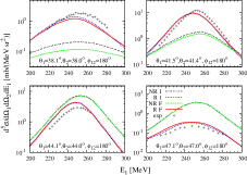
Figure 1: breakup - symmetric outgoing protons

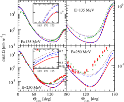
Figure 2: elastic pd scattering

References

- [1] E.P. Wigner, Annals Math. 40, 149 (1939)
- [2] K. Osterwalder, R. Schrader, Commun. Math. Phys. 31, 83 (1973)
- [3] K. Huang, H.A. Weldon, Phys. Rev. D11, 257 (1975)
- [4] P.A.M. Dirac, Rev. Mod. Phys. 21, 392 (1949)
- [5] S.N. Sokolov, A.N. Shatnyi, Theor. Math. Phys. 37, 1029 (1979)
- [6] T. Lin, C. Elster, W.N. Polyzou, W. Glockle, Phys. Lett. B660, 345 (2008)
- [7] V. Punjabi et al., Phys. Rev. C38, 2728 (1988)
- [8] H. Witała, J. Golak, R. Skibiński, W. Glöckle, H. Kamada, W.N. Polyzou, Phys. Rev. C 83, 044001 (2011)
- [9] H. Witała, J. Golak, R. Skibiński, W. Glöckle, H. Kamada, W.N. Polyzou, Phys. Rev. C 88, 069904 (2013)
- [10] K. Sekiguchi et al., Phys. Rev. C65, 034003 (2002)
- [11] K. Hatanaka et al., Phys. Rev. C 66, 044002 (2002)
- [12] Y. Maeda et al., Phys. Rev. C 76, 014004 (2007)