Calibrating general posterior credible regions

Abstract

An advantage of methods that base inference on a posterior distribution is that credible regions are readily obtained. Except in well-specified situations, however, there is no guarantee that such regions will achieve the nominal frequentist coverage probability, even approximately. To overcome this difficulty, we propose a general strategy that introduces an additional scalar tuning parameter to control the posterior spread, and we develop an algorithm that chooses this parameter so that the corresponding credible region achieves the nominal coverage probability.

Keywords and phrases: Bootstrap; coverage probability; Gibbs posterior; model misspecification; Monte Carlo.

1 Introduction

An advantage of methods that base their inference on a posterior distribution is that credible regions for the unknown parameters are readily available. It is common to require that the specified credibility level agrees, at least approximately, with the frequentist coverage probability, e.g., that the 95% credibility regions from the posterior are approximately 95% confidence regions. If so, then we say that the posterior credible region is calibrated. For well-specified Bayesian models, a Bernstein–von Mises theorem justifies a calibration claim, but when the model is misspecified, calibration often fails. For example, Kleijn and van der Vaart, (2012) derived a Bernstein–von Mises theorem for Bayesian posteriors under model misspecification, and pointed out that, even if the concentration target and rate are correct, misspecification can still cause a lack of calibration; see page 362 in their paper. Similarly, variational Bayes posteriors (e.g., Blei et al., 2017) often lack the calibration property, and correcting this is an important open problem.

To address this problem, we propose to augment the given posterior with an additional scalar tuning parameter that controls its spread. This is inspired by the literature on Gibbs posteriors, where data and the parameter of interest are connected via a loss function, like in (1), instead of a likelihood; see, e.g., Bissiri et al., (2016), Alquier et al., (2016), Zhang, (2006), Jiang and Tanner, (2008), and Syring and Martin, (2017). In such cases, a scale parameter must be specified to properly weight the information in the data relative to that in the prior, but this boils down to tuning the spread. A similar formulation is possible for other types of posterior distributions, not just Gibbs; see Section 2. Having introduced an extra parameter, we propose to select its value so that the corresponding posterior credible regions are calibrated in the sense described above, and we present a Monte Carlo algorithm to implement this idea.

Similar questions about scaling posterior distributions to address model misspecification have been considered recently in the literature. Ideas for choosing the posterior scaling are presented in Bissiri et al., (2016) and Holmes and Walker, (2017), including hierarchical Bayes and loss/information matching, and a novel idea in Grünwald and van Ommen, (2017). These proposals are reasonable, but they provide no guarantee that the corresponding posterior uncertainty quantification is meaningful. In contrast, our proposal here is designed specifically to calibrate posterior credible regions, at least approximately. Theoretical arguments support the soundness of our proposal, and numerical examples demonstrate both its versatility and effectiveness. Finer details about implementation of the method, along with two additional examples, are presented in the Supplementary Material.

2 Problem formulation

Suppose we have data $Z^{n}=(Z_{1},\ldots,Z_{n})$ consisting of independent and identically distributed observations with marginal distribution $P$; each $Z_{i}$ could be a vector or even a response–predictor variable pair, i.e., $Z_{i}=(X_{i},Y_{i})$. Throughout, we write $Pf$ for the expectation of a function $f(Z)$ with respect to $P$. The quantity of interest is $\theta=\theta(P)$, a feature of $P$, taking values in $\Theta\subseteq\mathbb{R}^{d}$ for some $d\geq 1$.

Consider the following general construction of a posterior distribution for inference on $\theta$. Start by connecting data $Z^{n}$ to a full set of parameters $\eta$ either through a statistical model for $P$, as in Bayesian settings, or through a suitable loss function, as in Gibbsian settings like in (1). Next, introduce a prior $\Pi$ for the full parameter $\eta$, and a scale $\omega>0$ to weight the information about $\eta$ in the data with that in the prior. Then combine the prior, scale, and likelihood/loss function to get a posterior for $\eta$ and, finally, get the corresponding marginal posterior for $\theta$, denoted by $\Pi_{n,\omega}$. In addition to Bayes and Gibbs posteriors, this construction includes variational Bayes posteriors, as discussed in the Supplementary Material, empirical Bayes, and others based on data-dependent priors (e.g., Martin and Walker, 2017; Hannig et al., 2016). Our one technical requirement is that $\Pi_{n,\omega}$ be consistent in the sense that, under $P$, it concentrates around $\theta(P)$ asymptotically for each fixed $\omega$. Consistency of $\Pi_{n,\omega}$ is not automatic, especially in cases of under- or misspecified models (e.g., Grünwald and van Ommen, 2017), but it is necessary if credible regions derived from it are to provide meaningful uncertainty quantification.

For concreteness, consider inference on the median $\theta$ of a distribution $P$. The median can be defined as the minimizer of the risk $R(\theta)=P\ell_{\theta}$, with loss function $\ell_{\theta}(z)=|z-\theta|$. This loss forms a connection between $Z^{n}$ and $\theta$, and a Gibbs posterior is defined as

$$\Pi_{n,\omega}(d\theta)\propto e^{-\omega nR_{n}(\theta)}\,\Pi(d\theta),$$ (1)

where $R_{n}(\theta)=\mathbb{P}_{n}\ell_{\theta}$ is the empirical version of the risk, $\omega>0$ is a scale parameter, and $\Pi$ is a prior for $\theta$; other examples of converting risk into a Gibbs posterior are given in Sections 4 and 5. As an alternative to the use of a loss function to connect data with the parameter of interest, one might specify a statistical model, e.g., $P$ is a gamma distribution with parameter $(\alpha,\beta)$. This determines a likelihood function $L_{n}(\eta)$ which, combined with a prior $\Pi$ for $\eta$, yields a posterior for $\theta$ given by

$$\Pi_{n,\omega}(A)\propto\int_{\{\eta:F_{\eta}^{-1}(1/2)\in A\}}L_{n}(\eta)^{\omega}\,\Pi(d\eta),$$

where $F_{\eta}$ denotes the corresponding gamma distribution function. The choice between these two approaches, or variations thereof, depends on the willingness of the data analyst to specify a full model, and on the objectives; the Gibbsian approach provides inference on the median but nothing else, with minimal modeling assumptions, whereas the Bayesian approach provides inference on virtually any feature, but with higher modeling and computational costs. In either case, the choice of $\omega$ is important.

Our proposed choice of scale is based on calibrating the posterior credible regions to be used for uncertainty quantification. Fix a level $\alpha\in(0,1)$ and, for concreteness, consider the highest posterior density credible regions defined as

$$C_{\omega,\alpha}(Z^{n})=\{\theta:\pi_{n,\omega}(\theta)\geq c_{\alpha}\},$$ (2)

where $\pi_{n,\omega}$ is the density function corresponding to the posterior $\Pi_{n,\omega}$, and $c_{\alpha}$ is chosen so that the $\Pi_{n,\omega}$-probability assigned to $C_{\omega,\alpha}(Z^{n})$ is equal to $1-\alpha$. Given that $\Pi_{n,\omega}$ is consistent, the scale parameter $\omega$ controls the spread of the posterior and, thus, the size of these credible regions. Our proposal is to choose $\omega$ so that the credible regions for $\theta$ are of the appropriate size to be calibrated, i.e., so that the coverage probability is approximately equal to $1-\alpha$.

3 Posterior calibration

3.1 Algorithm

Our goal is to select $\omega$ such that the corresponding posterior credible region are calibrated in the sense that the credibility level agrees with the coverage probability, at least approximately. To this end, for our desired significance level $\alpha\in(0,1)$, and our preferred credible region $C_{\omega,\alpha}(Z^{n})$ for $\theta$ as in (2), define the coverage probability function

$$c_{\alpha}(\omega;P)=P\{C_{\omega,\alpha}(Z^{n})\ni\theta(P)\},$$

i.e., the $P$-probability that the credible region $C_{\omega,\alpha}(Z^{n})$ contains the target $\theta(P)$. Then calibration requires that $\omega$ be such that

$$c_{\alpha}(\omega;P)=1-\alpha,$$ (3)

i.e., that the $100(1-\alpha)$% posterior credible region is also a $100(1-\alpha)$% confidence region. In practice we cannot solve this equation because we do not know $P$. The approach described below is designed to get around this roadblock.

To build up our intuition, start by assuming that $P$ is known. Even in this case, numerical methods are generally required to solve (3). One can use stochastic approximation (e.g., Robbins and Monro, 1951) with iterations

$$\omega^{(t+1)}=\omega^{(t)}+\kappa_{t}\{\hat{c}_{\alpha}(\omega^{(t)}\mid P)-(1-\alpha)\},\hskip 28.45274ptt\geq 0,$$ (4)

where $\hat{c}_{\alpha}(\omega\mid P)$ is a Monte Carlo approximation to the coverage probability, obtained by simulating new copies of the data $Z^{n}$ from $P$, and $(\kappa_{t})$ is a non-stochastic sequence such that $\sum_{t}\kappa_{t}=\infty$ and $\sum_{t}\kappa_{t}^{2}<\infty$; in our examples we use $\kappa_{t}=(t+1)^{-0.51}$. If $c_{\alpha}(\omega;P)$ is continuous and monotone decreasing in $\omega$, as would be expected even for moderate $n$ under our consistency assumption, at least on an interval away from 0, then the main result in Robbins and Siegmund, (1971) implies $\omega^{(t)}\to\omega^{\star}$ $P$-almost surely, as $t\to\infty$, where $\omega^{\star}$ is the solution to (3).

When $P$ is unknown, the proposed approach changes in two ways. First, since it is not possible to sample new copies of $Z^{n}$ from $P$, we replace simulation from $P$ with that from $\mathbb{P}_{n}$, i.e., we sample with replacement from the observed data $Z^{n}$. Second, since we also do not know $\theta(P)$, we cannot check if a given credible region $C_{\omega,\alpha}(Z^{n})$ covers it, so we use $\theta(\mathbb{P}_{n})$ in place of $\theta(P)$. This results in an empirical version of $c_{\alpha}(\omega;P)$, namely, $c_{\alpha}(\omega;\mathbb{P}_{n})=\mathbb{P}_{n}\{C_{\omega,\alpha}(Z^{n})\ni\theta(\mathbb{P}_{n})\}$, and then our proposal is to find $\omega$ such that

$$c_{\alpha}(\omega;\mathbb{P}_{n})=1-\alpha.$$ (5)

In practice, we cannot evaluate $c_{\alpha}(\omega;\mathbb{P}_{n})$ either, but the bootstrap provides a Monte Carlo estimator, $\hat{c}_{\alpha}(\omega;\mathbb{P}_{n})$. We can solve (5) using the stochastic approximation procedure described above for the known-$P$ case. Collectively, the steps in Algorithm 1 make up our general posterior calibration (GPC) algorithm. R code for several examples is available at https://github.com/nasyring/GPC.

Fix a convergence tolerance $\varepsilon>0$ and an initial guess $\omega^{(0)}$ of the calibration parameter. Take $B$ bootstrap samples $\tilde{Z}_{1}^{n},\ldots,\tilde{Z}_{B}^{n}$ of size $n$. Set $t=0$ and do:

1. Construct credible regions $C_{\omega^{(t)},\alpha}(\tilde{Z}_{b}^{n})$ for each $b=1,\ldots,B$.

2. Evaluate the empirical coverage probability $\hat{c}_{\alpha}(\omega^{(t)};\mathbb{P}_{n})$.

3. If $\bigl{|}\hat{c}_{\alpha}(\omega^{(t)};\mathbb{P}_{n})-(1-\alpha)\bigr{|}<\varepsilon$, then stop and return $\omega^{(t)}$ as the output; otherwise, update $\omega^{(t)}$ to $\omega^{(t+1)}$ according to (4), set $t\leftarrow t+1$, and go back to Step 1.

Algorithm 1 — General Posterior Calibration.

In most applications, the credible regions $C_{\omega,\alpha}(Z^{n})$ are unavailable in closed form, so posterior sampling will be needed. In the basic version of the algorithm presented here, this posterior sampling must be repeated for each bootstrap sample and each GPC iteration, which may or may not be prohibitive in a particular application. But there are modifications that can be made to speed up the algorithm’s performance. For example, the bootstrap computations of $\hat{c}_{\alpha}(\omega;\mathbb{P}_{n})$ can be done in parallel, and we have implemented such a routine for the problem in Section 4. There, with $n=100$ data points, $B=200$ bootstraps, and $M=2000$ posterior samples, our parallelized implementation met the calibration criterion in less than 5 seconds on an ordinary desktop computer. In addition, the frequency of posterior sampling can be reduced by adopting an importance sampling strategy when the change $\omega^{(t)}\to\omega^{(t+1)}$ is small.

3.2 Theoretical support

There are two theoretical questions of interest. First, does a solution $\omega^{\star}$ to (3) exist? Second, do the iterates from the proposed algorithm converge to $\omega^{\star}$? The discussion here will focus primarily on the first question, but this analysis will also shed light on the second question and on some other existing methods for setting the scale $\omega$.

We start with a simple case to build some intuition. Let $Z^{n}$ be an independent sample of size $n$ from a normal distribution with mean $\theta$ and variance $\psi^{2}$; the goal is inference on the mean. However, suppose that we fix the variance at $\sigma^{2}\neq\psi^{2}$, i.e., a misspecified model. If we construct a posterior $\Pi_{n,\omega}$ using a scaling parameter $\omega$ and a flat prior, then the credible intervals are of the standard form: $\bar{Z}\pm z_{\alpha}(\omega^{-1}\sigma^{2}n^{-1})^{1/2}$, where $z_{\alpha}$ is the upper $\alpha$ quantile of the standard normal distribution. Clearly, to achieve the desired calibration, one must take $\omega=\sigma^{2}/\psi^{2}$. Therefore, at least in this simple example, there is a solution to (3), and note that it does not depend on $\alpha$. Similar conclusions can be reached more generally and from different perspectives, as we discuss below.

Next, suppose the $d$-dimensional $\theta=\theta(P)$ is defined via a risk function $R(\theta)=P\ell_{\theta}$, so that $\theta(P)=\arg\min R(\theta)$. Then a Gibbs posterior $\Pi_{n,\omega}$ is defined as in (1), where $R_{n}(\theta)=\mathbb{P}_{n}\ell_{\theta}$ is the empirical risk. Under suitable regularity conditions (e.g., Chernozhukov and Hong, 2003; Müller, 2013), the Gibbs posterior will be approximately normal, centered at $\theta(\mathbb{P}_{n})=\arg\min R_{n}(\theta)$, with asymptotic covariance matrix $\omega^{-1}\Sigma_{n}$, where $\Sigma_{n}=(nV_{\theta(\mathbb{P}_{n})})^{-1}$ and $V_{\theta}$ is the second derivative matrix of $R(\theta)$. So, asymptotically, the $100(1-\alpha)$% credible region $C_{\omega,\alpha}(Z^{n})$ is

$$\bigl{[}\theta:\omega\{\theta-\theta(\mathbb{P}_{n})\}^{\top}\Sigma_{n}^{-1}\{\theta-\theta(\mathbb{P}_{n})\}\leq q_{\alpha}\bigr{]},$$

where $q_{\alpha}$ is the upper $\alpha$ quantile of a chi-square distribution with $d$ degrees of freedom. And for the above credible region, the coverage probability function is

$$c_{\alpha}(\omega;P)=G_{n}(q_{\alpha}/\omega),$$

where $G_{n}$ is the distribution function of $\{\theta(\mathbb{P}_{n})-\theta(P)\}^{\top}\Sigma_{n}^{-1}\{\theta(\mathbb{P}_{n})-\theta(P)\}$ under independent sampling of $Z^{n}$ or, equivalently, $\mathbb{P}_{n}$ from $P$. This asymptotic representation of the coverage probability as a smooth non-increasing function of $\omega$ reveals that a solution to (3) exists, at least for sufficiently large $n$.

To see what the solution $\omega$ looks like, we push this argument further. Under the same regularity conditions, the M-estimator $\theta(\mathbb{P}_{n})$ has an asymptotic representation

$$\theta(\mathbb{P}_{n})=\theta(P)+\Psi_{n}^{\text{c}}\,\xi+o_{P}(1),$$

where $\xi$ is a vector of independent standard normals and $\Psi_{n}^{\text{c}}$ is the Cholesky factor of the sandwich covariance matrix $\Psi_{n}=n^{-1}V_{\theta(P)}^{-1}\{P\dot{\ell}_{\theta(P)}\dot{\ell}_{\theta(P)}^{\top}\}V_{\theta(P)}^{-1}$, with $\dot{\ell}_{\theta}$ the derivative of $\theta\mapsto\ell_{\theta}$. This implies that

$$\bigl{|}G_{n}(q_{\alpha}/\omega)-{\rm pr}(\xi^{\top}\Psi_{n}^{\text{c}\top}\,\Sigma_{n}^{-1}\Psi_{n}^{\text{c}}\,\xi\leq q_{\alpha}/\omega)\bigr{|}\to 0,\quad n\to\infty,$$

pointwise and also uniformly in $\omega$, at least over a set bounded away from 0. Therefore, if the generalized information equality (Chernozhukov and Hong, 2003) holds, i.e., if $\Sigma_{n}=b\Psi_{n}$ for a constant $c>0$, then (3) holds asymptotically with $\omega=b$; compare this to the $\sigma^{2}/\psi^{2}$ result in the toy example. More generally, with no information proportionality property, (3) will hold asymptotically for some $\omega$ greater than the smallest eigenvalue of $\{\Psi_{n}^{\text{c}\top}\,\Sigma_{n}^{-1}\Psi_{n}^{\text{c}}\}^{-1}$. Therefore, under general conditions, a solution to (3) exists, at least asymptotically and, as in the toy example above, it does not depend on $\alpha$.

The second question, about whether our proposed algorithm identifies a solution, is more difficult to answer. Individually, the workhorses of the GPC algorithm, namely, stochastic approximation, bootstrap, and Monte Carlo, are sound computational tools, but a simultaneous analysis of the three working in tandem is formidable. However, if we take the posterior computations and stochastic approximation to be exact, focusing only on the bootstrap component, then the above analysis provides some insight. That the coverage probability can be characterized, asymptotically, via a distribution function means that solving for $\omega$ is equivalent to finding a quantile of the distribution of an approximate pivot. And it is well known (e.g., Davison and Hinkley, 1997, p. 39–41) that the bootstrap approximation is valid for such tasks under very mild conditions. Therefore, at least asymptotically, theory suggests that our algorithm produces calibrated credible regions. Moreover, the numerical examples presented here and in the Supplementary Material suggest that GPC achieves calibration, exactly or conservatively, even in finite samples. But a scaling approach like ours cannot correct a misspecified shape, and the same goes for Holmes and Walker, (2017) and Grünwald and van Ommen, (2017), so our calibrated posterior will generally be too wide in some direction; see Section 3.3.

Finally, as a reviewer pointed out, there are close connections between those $\omega$ values that achieve calibration and those in Grünwald, (2012) and Grünwald and Mehta, (2017) achieve fast rates of convergence. This connection has several important implications. In particular, it suggests that there may be a unified framework for generalized posteriors where, at least asymptotically, a single choice of scaling achieves all the desired inferential goals. But calibration is more delicate than a fast convergence rate, and this difference manifests here in that the calibration theory requires setting $\omega$ exactly at a threshold analogous to that given in Grünwald and Mehta, (2017), whereas the SafeBayes algorithm in Grünwald and van Ommen, (2017) plays it safe by setting the scale factor slightly less than that threshold. In the finite-dimensional cases being considered here, there is no serious risk in setting $\omega$ at the threshold to achieve both calibration and optimal convergence rates. However, in more complex infinite-dimensional cases, one should expect to risk sub-optimal rates in exchange for valid uncertainty quantification (e.g., Martin, 2017). These interesting observations deserve further investigation.

3.3 Illustration

Example 1 in Ribatet et al., (2012) presents a case where $\{Y(x):x\in\mathbb{R}\}$ is a Gaussian process with mean $\mu\in\mathbb{R}$ and covariance function $K(x,x^{\prime})=\tau e^{-\kappa|x-x^{\prime}|}$, where $\kappa>0$ is known but $\theta=(\mu,\tau)$ is unknown. They present two Bayesian analyses, one based on the full likelihood and one based on a pairwise composite likelihood, the latter motivated by simpler computations. But since the composite likelihood is misspecified in that it treats all pairs of observations as independent, the uncertainty measures it produces are overly optimistic, i.e., the posterior is too concentrated.

To illustrate our scaling method, we reproduce the simulation summarized in Figure 1 of Ribatet et al., (2012). Our Figure 1 summarizes the full posterior, the composite likelihood-based posterior, and our calibrated version of the latter, where the scaling parameter return by our posterior calibration algorithm is $\omega=0.015$. The two marginal posterior density plots in Panels (a) and (b) match what is shown in Ribatet et al., (2012). Our calibrated posterior exactly matches the full posterior for $\mu$, but is a bit wider than that for $\tau$. Panel (c) summarizes the joint posteriors and helps explain what is going on. The composite posterior is too tightly concentrated, but also is more circular than the full posterior. Our scaling approach stretches the composite posterior’s roughly circular contours till they achieve calibration, and these will necessarily exceed the narrowest part of the full posterior’s elliptical contours, as in Panel (c).

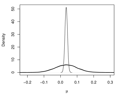
(a) Marginal density for $\mu$

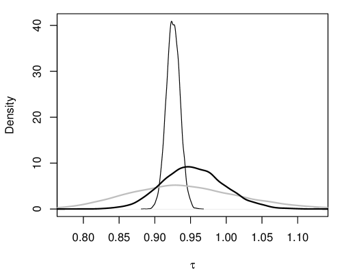
(b) Marginal density for $\tau$

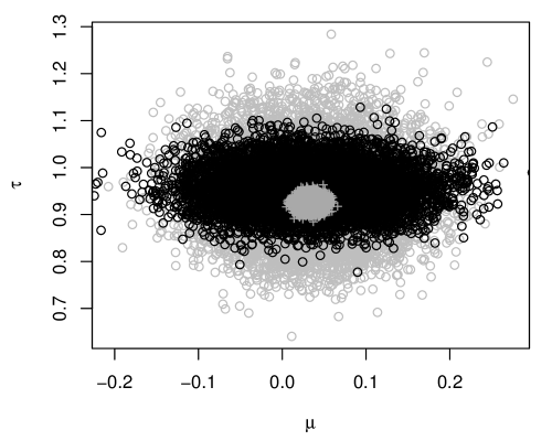
(c) Samples of $(\mu,\tau)$

Figure 1: Results for the example in Section 3.3. Panels (a) and (b) show the Bayesian (thick black line), composite (thin black line), and scaled composite (gray line) posterior densities for $\mu$ and $\tau$, respectively. In Panel (c), tight gray cluster in the foreground is the pairwise composite posterior, black is the Bayesian posterior, and wider gray cluster in the background is the scaled composite posterior, with $\omega=0.015$.

4 Quantile regression example

In quantile regression, for fixed $\tau\in(0,1)$, we are interested in the $\tau^{\text{th}}$ quantile of the response $Y\in\mathbb{R}$, given the covariates $X\in\mathbb{R}^{p+1}$, expressed as

$$Q_{\tau}(Y\mid X)=X^{\top}\theta,$$ (6)

where dimension $p+1$ represents an intercept and $p$ covariates. In (6), the vector $\theta$ depends on $\tau$ but we will omit this dependence for simplicity. Inference on the quantile regression coefficient $\theta$ may be carried out using asymptotic approximations (Koenker, 2005, Theorem 4.1) or the bootstrap (Horowitz, 1998). A Bayesian approach would also be attractive, but no distributional form is given in (6) so a likelihood requires further specification. An option considered by several authors (e.g., Yu and Moyeed, 2001; Sriram et al., 2013; Sriram, 2015) is to use a misspecified asymmetric Laplace likelihood. This corresponds to a Gibbs posterior (1) using the empirical risk

$$R_{n}(\theta)=\frac{1}{n}\sum_{i=1}^{n}|(Y_{i}-X_{i}^{\top}\theta)(\tau-1_{Y_{i}<X_{i}^{\top}\theta})|,$$ (7)

where $1_{A}$ denotes the indicator function for $A$. Here we consider $\tau=0.5$.

To demonstrate the performance of our proposed scaling algorithm, we revisit a simulation example presented in Yang and He, (2012). The model they consider is

$$Y_{i}=\theta_{0}+\theta_{1}\,X_{i}+e_{i},\quad i=1,\ldots,n,$$

where $\theta_{0}=2$, $\theta_{1}=1$, $e_{i}\overset{\text{\tiny iid}}{\,\sim\,}{\sf N}(0,4)$, and $X_{i}+2\overset{\text{\tiny iid}}{\,\sim\,}{\sf ChiSq}(2)$. Yang and He, (2012) showed numerically that their Bayesian empirical likelihood method produced credible intervals with approximate coverage near the nominal 95% level. They also show their method produces credible intervals with shorter average lengths than a Gibbs posterior with $\omega$ equal to the average absolute residuals calculated using the usual quantile regression parameter estimates. The results for these methods are presented in Table 1, along with the results from the posterior intervals scaled by our algorithm.

There are two key observations to be made. First, our method calibrates the credible intervals to have exact 95% coverage across the range of $n$, while the other methods tend to over-cover. Second, our credible intervals tend to be shorter than those of the other methods, especially for $n=100$. All three methods have a $n^{-1/2}$ convergence rate so, for large $n$, we cannot expect to see substantial differences between the various methods. Therefore, the small-$n$ case should be the most important and, at least in this case, the credible intervals calibrated using our algorithm are the best.

		Coverage Probability $\times 100$						Average Length $\times 100$
$n$		BEL.s	BDL	Normal	$\omega\equiv 0.8$	GPC		BEL.s	BDL	Normal	$\omega\equiv 0.8$	GPC
$100$	$\theta_{0}$	$97$	$98$	95	96	95		$106$	$111$	100	100	91
	$\theta_{1}$	$98$	$98$	98	98	95		$58$	$58$	55	52	47
$400$	$\theta_{0}$	$95$	$98$	95	95	95		$50$	$55$	50	49	46
	$\theta_{1}$	$97$	$98$	97	96	95		$26$	$28$	25	25	23
$1600$	$\theta_{0}$	$96$	$97$	96	95	95		$25$	$28$	25	24	23
	$\theta_{1}$	$96$	$98$	96	96	95		$13$	$14$	12	12	11

Table 1: Comparison of $95\%$ posterior credible intervals of the median regression parameters from five methods: BEL.s and BDL are two methods presented in Yang and He, (2012); Normal is the confidence interval computed using the asymptotic normality of the M-estimator; $\omega\equiv 0.8$ is the scaled posterior with fixed $\omega$; and our GPC. Coverage probability and average interval lengths are based on $5000$ simulated data sets.

Finally, considering that in smooth models we expect $\omega$ to account for the difference in asymptotic variance between the posterior and the M-estimator, it is reasonable to ask if we need a calibration algorithm at all, i.e., can we get by with a fixed value of $\omega$ based on these asymptotic variances? A comparison of the asymptotic variance of the posterior with that of the M-estimator shows that $\Sigma_{n}\approx 0.80\Psi_{n}$; therefore, we can take $\omega\equiv 0.80$ in an attempt to calibrate posterior credible intervals with a fixed scaling. Table 1 shows that our algorithm is still better than using a fixed scale based on asymptotic normality, especially at smaller sample sizes where the normal approximation is less justifiable.

5 Application

Polson and Scott, (2011) propose to convert the objective function of the support vector machine into a sort of log-likelihood function for the purpose of carrying out a Bayesian analysis. Let $y$ be a binary $n$-vector, with $y_{i}\in\{-1,+1\}$ for $i=1,\ldots,n$, and $X$ a $n\times p$ matrix of predictors, including a column of ones for an intercept. Then the support vector machine seeks to find $\theta=(\theta_{0},\ldots,\theta_{p-1})\in\mathbb{R}^{p}$ to minimize

$$D_{n}(\theta)=nR_{n}(\theta)+\nu^{-1}\sum_{j=0}^{p-1}\bigl{|}\theta_{j}/\sigma_{j}\bigr{|},$$

where $\nu>0$ is a tuning parameter, $\sigma_{j}$ is the standard deviation of the $j$th column of $X$, with $\sigma_{0}\equiv 1$, and $R_{n}(\theta)=n^{-1}\sum_{i=1}^{n}2\max\{0,1-y_{i}x_{i}^{\top}\theta\}$, with $x_{i}^{\top}$ the $i$th row of $X$. Then Polson and Scott, (2011) propose a pseudo-posterior distribution $\Pi_{n}$ with density function proportional to $\exp\{-D_{n}(\theta)\}$, which amounts to combining a pseudo-likelihood $L_{n}(\theta)=\exp\{-nR_{n}(\theta)\}$ with independent Laplace-type prior, $\Pi$, for $\theta$. Their motivation is that, while the support vector machine only provides point estimates, this Bayesian formulation also offers uncertainty quantification. However, as this support vector machine-driven posterior has no connection to a model that describes the variability in the data, it is not clear what the uncertainty measures derived from this posterior represent; certainly there is no reason to expect that posterior credible regions derived from it will be calibrated in the sense considered here. To overcome this, we can introduce the scale parameter $\omega$, get a posterior $\Pi_{n,\omega}$ for $\theta$, and then $\omega$ can be chosen according to the calibration algorithm proposed above, thereby calibrating the corresponding credible region.

To illustrate this, consider the South African heart disease data presented analyzed in Section 4.4.2 of Hastie et al., (2009). The binary response is the presence/absence of myocardial infarction. We focus here on a subset of predictors, in Table 4.3 of Hastie et al., (2009), determined to have a non-negligible association with the response, namely, tobacco use, cholesterol level, family history of heart disease, and age. The Gibbs sampler in Polson and Scott, (2011) can be easily modified to incorporate our scaling $\omega$, and our calibration algorithm yields $\omega\approx 0.09$, for a target 95% coverage; here we fix $\nu=10$. Figure 2 shows the estimated marginal density functions for each of $\theta_{1}$, $\theta_{2}$, and $\theta_{3}$ based on the Polson and Scott proposal, with $\omega=1$, and ours with $\omega=0.09$; the plot for $\theta_{4}$ looks similar, so is omitted for the sake of space. These plots indicate that, compared to our suitably calibrated posterior, Polson and Scott’s posterior is far too narrow, exaggerating the precision of their inferences.

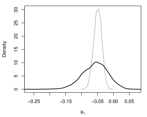
(a) Tobacco use, $\theta_{1}$

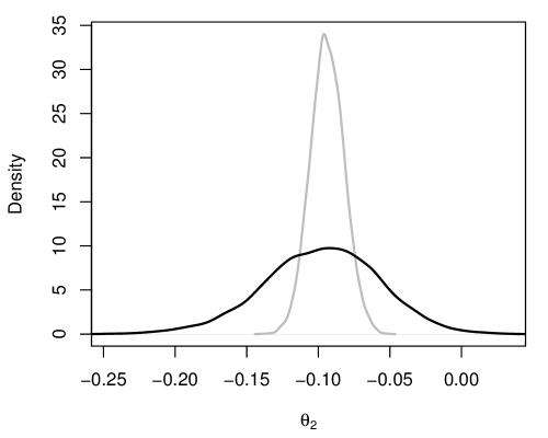
(b) Cholesterol, $\theta_{2}$

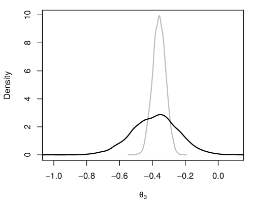
(c) Family history, $\theta_{3}$

Figure 2: Marginal posterior densities in the support vector machine-based model; Polson and Scott, (2011), gray, and our calibrated version, black.

 

Supplementary material

Linear regression example

Consider the linear regression model for data $(X_{i},Y_{i})\in\mathbb{R}^{p}\times\mathbb{R}$,

$$Y_{i}=\beta_{0}+X_{i}^{\top}\beta+\sigma\,e_{i},\quad i=1,\ldots,n,$$ (8)

where $\beta\in\mathbb{R}^{p}$ is the vector of slope coefficients, $\sigma>0$ is an unknown scale parameter, and $e_{1},\ldots,e_{n}$ are assumed to be independent and identically distributed normal random variables with mean $0$ and variance $1$. Suppose, however, that the constant error variance assumption is violated, in particular, the variance of $e_{i}$ is $\|X_{i}\|$, $i=1,\ldots,n$. Our choice of predictor-dependent variance is a less-stylized version of that in Grünwald and van Ommen, (2017). The proposed model is, therefore, misspecified, but our goal is still to obtain calibrated inference on $\theta=(\beta_{0},\beta)$.

The Jeffreys prior with density $\pi(\eta)\propto(\sigma^{2})^{-3/2}$ is a reasonable default choice (Ibrahim and Laud, 1991) for the full parameter $\eta=(\theta,\sigma^{2})$. Since this prior is probability-matching for the location-scale model (e.g., Datta and Mukerjee, 2004), we may expect that the posterior credible intervals would be approximately calibrated for our linear regression. However, for a misspecified model, calibration might fail; in fact, as shown in Table 2, the credible intervals are too narrow and tend to undercover.

To investigate the performance of our proposed posterior calibration method, we carry out a simulation study. We simulated data sets of $n=50$ observations. Each $X_{i}\in\mathbb{R}^{3}$ is multivariate normal with zero mean and unit variance for each element, and correlation $0.5$ for $X_{i1}$ and $X_{i2}$ and zero otherwise. To sample $Y_{i}$ we use $\beta_{0}=0$, $\beta=(1,2,-1)^{\top}$, and $\sigma=1$. Although the error variance contains $\|X_{i}\|$, the White test for constant variance does not detect the heteroscedasticity reliably. Table 2 shows the estimated coverages and mean lengths of several posterior credible intervals for the components of $\theta$. Besides those scaled by the general posterior calibration algorithm, we consider a misspecified Bayes approach that fixes $\omega\equiv 1$, and posteriors with scale $\omega$ chosen by the method in Holmes and Walker, (2017) and the method in (Grünwald and van Ommen, 2017, Algorithm 1). Table 2 shows that for this example SafeBayes performs similarly to general posterior calibration, while the method in Holmes and Walker, (2017) does not improve upon the misspecified Bayesian model in terms of calibration.

To perform general posterior calibration we begin by fitting the linear model to the data and generating $B=200$ bootstrap resampled data sets, $(Y_{b}^{\star},X_{b}^{\star})$ for $b=1,...,B$, by selecting $n$ rows with replacement from $Y$ and $X$. For each bootstrap sample, $(Y_{b}^{\star},X_{b}^{\star})$, we fit the linear model and produce bootstrap estimates $\beta_{0,b}^{\star}$ and $\beta_{b}^{\star}$. We set $\omega=\omega_{0}$ and use a Gibbs sampler to generate $M=2000$ samples from the posterior distribution of $(\theta,\sigma^{2})$, given $\omega$ and $(Y_{b}^{\star},X_{b}^{\star})$ for each of the $B$ bootstrap resampled data sets. From these $B$ sets of $M$ posterior samples, we compute $B$ credible intervals for $\beta_{0}$ and each element of $\beta$. Simple equi-tailed credible intervals can be used, but we found that highest posterior density credible intervals are more accurate in practice. The average of the bootstrap estimates, $\tilde{\beta}=B^{-1}\sum_{b=1}^{B}\hat{\beta}^{\star}_{b}$, is used in place of the unknown $\beta$ to determine coverage proportions for each posterior credible interval. Then

$$\hat{c}_{\alpha}(\omega;\mathbb{P}_{n})=\frac{1}{B}\sum_{b=1}^{B}1\{C_{\omega,\alpha}(Y_{b}^{\star},X_{b}^{\star})\ni\tilde{\beta}\},$$

where $C_{\omega,\alpha}(Y_{b}^{\star},X_{b}^{\star})$ is the highest posterior density credible set for $\beta$. Then, the stochastic approximation step is used to update $\omega$ according $(4)$. The algorithm converges when $\hat{c}_{\alpha}(\omega;\mathbb{P}_{n})-(1-\alpha)<\varepsilon$, and we take $\varepsilon=B^{-1}$.

The implementation of general posterior calibration can be modified to increase accuracy, decrease runtime, or perhaps both. In this linear model example, general posterior calibration runs faster for a Gibbsian posterior based on the empirical risk function $R_{n}(\beta_{0},\beta)=n^{-1}\sum_{i=1}^{n}(Y_{i}-\beta_{0}-X_{i}^{\top}\beta)^{2}$ than for the misspecified Bayes posterior due to the lack of the nuisance variance parameter $\sigma^{2}$ in the former.

In general, the posterior calibration algorithm can be accelerated by decreasing $M$, $B$, or both, but reducing either number will also reduce the quality of the empirical coverage proportions $\hat{c}_{\alpha}(\omega;\mathbb{P}_{n})$. In our implementation of general posterior calibration, the posterior is sampled every time $\omega$ is updated. However, it may be faster to sample the posterior $M$ times for $\omega_{0}$ and subsequently use importance sampling to update the posterior samples each time $\omega$ is updated.

The above simulation was repeated with $\kappa_{t}=ct^{-0.51}$ for $c=1,2,$ and $5$. While there were no appreciable differences in credible interval coverage proportions or lengths for the different choices of $\kappa_{t}$, the algorithm ran in about 40, 30, and 50 seconds with $c=1$, $c=2$, and $c=5$, respectively, suggesting that an optimal choice of $\kappa_{t}$ could improve general posterior calibration runtime. These run-times could also be reduced via parallelization, as we did for the example in Section 4 of the main text.

We used our general posterior calibration algorithm to select $\omega$ to calibrate $95\%$ credible regions, simultaneously, for all three elements of $\beta$. However, we also calibrate $100(1-\alpha)\%$ credible intervals for any confidence level $\alpha$ with the same $\omega$. For instance, $90\%$ and $80\%$ credible intervals were also calibrated to a similar degree of accuracy compared with $95\%$ credible intervals. This confirms the theoretical claims made in Section 3.2 of the main text.

It is interesting to compare $\omega$ values generated by different algorithms. The mean $\omega$ values are 0.80 and 0.77 for general posterior calibration and Grünwald–van Ommen. General posterior calibration is less variable than Grünwald–van Ommen with standard deviation 0.05 for the former and 0.15 for the latter. The method in Holmes–Walker generates $\omega$ values that average $1.29$, significantly different than those from general posterior calibration and Grünwald–van Ommen.

			$\beta_{0}$	$\beta_{1}$	$\beta_{2}$	$\beta_{3}$
Misspecified Bayes	coverage		94	89	88	87
	length		99	116	116	101
General posterior calibration	coverage		98	94	94	93
	length		117	136	136	118
SafeBayes	coverage		96	93	94	92
	length		119	140	139	121
Holmes and Walker	coverage		91	84	80	82
	length		87	101	101	87

Table 2: Empirical coverage probability of $95\%$ credible intervals and average interval lengths calculated using 5000 simulations from the linear regression model. All values are multiplied by $100$.

Finite mixture model example

Variational inference offers a competing method to Markov chain Monte Carlo for approximating posterior distributions. This approach specifies a family of distributions, often a normal family, as candidate posteriors and then chooses the parameters of that family to minimize the Kullback–Leibler divergence from the true posterior. The variational posterior is simple by construction and, if carefully chosen, will be consistent (e.g., Wang and Titterington, 2005), but as noted in Blei et al., (2017), misspecification causes the variational posterior variance to be too small.

As an example, we consider the normal mixture model presented in Blei et al., (2017), i.e., $Y_{1},\ldots,Y_{n}$ are independent and identically distributed from

$$\sum_{k=1}^{K}\pi_{k}{\sf N}(\mu_{k},\sigma_{k}^{2}).$$ (9)

The full parameter $\eta$ consists of the mixture weights $(\pi_{1},\ldots,\pi_{K})$, means $(\mu_{1},\ldots,\mu_{K})$, and variances $(\sigma_{1}^{2},\ldots,\sigma_{K}^{2})$, but we will consider inference only on the means. We can construct a variational posterior for $\eta$ following Algorithm 2 in Blei et al., (2017), which approximates the posterior by a multivariate normal distribution. The additional scale factor $\omega$ in our modified variational posterior $\Pi_{n,\omega}$ only adjusts the overall scale of this multivariate normal distribution. Therefore, if $m_{1},\ldots,m_{K}$ and $v_{1},\ldots,v_{K}$ are the means and variances, respectively, of this variational posterior for the mixture means $\mu_{1},\ldots,\mu_{K}$, then the corresponding $\omega$-scaled variational posterior $100(1-\alpha)$% credible intervals are of the form

$$\mu_{k}\pm z_{\alpha/2}^{\star}\,\omega\,v_{k}^{1/2},\quad k=1,\ldots,K.$$

It is straightforward to apply our general posterior calibration algorithm to variational posteriors; the computational investment is in carrying out the optimization needed for the variational approximation at each bootstrap step, but then the credible intervals are available in closed-form so no posterior sampling is needed.

We claim that the general posterior calibration algorithm will properly scale the variational posterior, calibrating the corresponding credible intervals, correcting the under-estimation of variance noted in Blei et al., (2017). To demonstrate this, we carry out a simple simulation study. We take $K=2$, $\pi_{1}=\pi_{2}=1/2$, $(\mu_{1},\mu_{2})=(-2,2)$, and $\sigma_{1}=\sigma_{2}=1$. Table 3 shows the empirical coverage probabilities and mean lengths of the 95% credible intervals based on Algorithm 2 in Blei et al., (2017) and our general posterior calibration algorithm. Apparently, our algorithm corrects the underestimated variance of the variational posterior, producing credible intervals that are slightly conservative.

			$\mu_{1}$		$\mu_{2}$
General posterior calibration	coverage		96		96
	length		67		67
Variational posterior	coverage		92		92
	length		55		55

Table 3: Empirical coverage probabilities and average lengths of the 95% credible intervals for $(\mu_{1},\mu_{2})$ based on our general posterior calibration algorithm and the variational posterior in Blei et al., (2017) over 5000 simulated data sets from the mixture model (9). All results are multiplied by $100$.

References

- Alquier et al., (2016) Alquier, P., Ridgway, J., and Chopin, N. (2016). On the properties of variational approximations of Gibbs posteriors. J. Mach. Learn. Res., 17:1–41.
- Bissiri et al., (2016) Bissiri, P., Holmes, C., and Walker, S. (2016). A general framework for updating belief distributions. J. R. Stat. Soc. Ser. B Stat. Methodol., 78(5):1103–1130.
- Blei et al., (2017) Blei, D. M., Kucukelbir, A., and McAuliffe, J. D. (2017). Variational inference: a review for statisticians. J. Amer. Statist. Assoc., 112(518):859–877.
- Chernozhukov and Hong, (2003) Chernozhukov, V. and Hong, H. (2003). An MCMC approach to classical estimation. Journal of Econometrics, 115:293–346.
- Datta and Mukerjee, (2004) Datta, G. and Mukerjee, R. (2004). Probability Matching Priors: Higher Order Asymptotics. Springer, New York.
- Davison and Hinkley, (1997) Davison, A. C. and Hinkley, D. V. (1997). Bootstrap Methods and their Application, volume 1. Cambridge University Press, Cambridge.
- Grünwald, (2012) Grünwald, P. (2012). The safe Bayesian: learning the learning rate via the mixability gap. In Algorithmic Learning Theory, volume 7568 of Lecture Notes in Comput. Sci., pages 169–183. Springer, Heidelberg.
- Grünwald and Mehta, (2017) Grünwald, P. and Mehta, N. (2017). Faster rates for general unbounded loss functions: from ERM to generalized Bayes. Unpublished manuscript, arXiv:1605.00252.
- Grünwald and van Ommen, (2017) Grünwald, P. and van Ommen, T. (2017). Inconsistency of Bayesian inference for misspecified linear models, and a proposal for repairing it. Bayesian Anal., 12(4):1069–1103.
- Hannig et al., (2016) Hannig, J., Iyer, H., Lai, R., and Lee, T. (2016). Generalized fiducial inference: A review and new results. J. Amer. Statist. Assoc., 111:1346–1361.
- Hastie et al., (2009) Hastie, T., Tibshirani, R., and Friedman, J. (2009). The Elements of Statistical Learning. Springer-Verlag, New York, 2nd edition.
- Holmes and Walker, (2017) Holmes, C. C. and Walker, S. G. (2017). Assigning a value to a power likelihood in a general Bayesian model. Biometrika, 104(2):497–503.
- Horowitz, (1998) Horowitz, J. (1998). Bootstrap methods for median regression models. Econometrica, 66:1327–1351.
- Ibrahim and Laud, (1991) Ibrahim, J. G. and Laud, P. W. (1991). On Bayesian analysis of generalized linear models using Jeffreys’s prior. J. Amer. Statist. Assoc., 86(416):981–986.
- Jiang and Tanner, (2008) Jiang, W. and Tanner, M. A. (2008). Gibbs posterior for variable selection in high-dimensional classification and data mining. Ann. Stat., 36(5):2207–2231.
- Kleijn and van der Vaart, (2012) Kleijn, B. and van der Vaart, A. (2012). The Bernstein-Von-Mises theorem under misspecification. Electron. J. Stat., 6:354–381.
- Koenker, (2005) Koenker, R. (2005). Quantile Regression. Econometric Society Monographs, volume 38. Cambridge Univ. Press, Cambridge.
- Martin, (2017) Martin, R. (2017). Comment on the article by van der Pas, Szabó, and van der Vaart. Bayesian Anal., 12(4):1254–1258.
- Martin and Walker, (2017) Martin, R. and Walker, S. G. (2017). Empirical priors for target posterior concentration rates. Unpublished manuscript, arXiv:1604.05734.
- Müller, (2013) Müller, U. K. (2013). Risk of Bayesian inference in misspecified models, and the sandwich covariance matrix. Econometrica, 81(5):1805–1849.
- Polson and Scott, (2011) Polson, N. G. and Scott, S. L. (2011). Data augmentation for support vector machines. Bayesian Anal., 6(1):1–23.
- Ribatet et al., (2012) Ribatet, M., Cooley, D., and Davison, A. C. (2012). Bayesian inference from composite likelihoods, with an application to spatial extremes. Statist. Sinica, 22(2):813–845.
- Robbins and Monro, (1951) Robbins, H. and Monro, S. (1951). A stochastic approximation method. Ann. Math. Stat., 22:400–407.
- Robbins and Siegmund, (1971) Robbins, H. and Siegmund, D. (1971). A convergence theorem for non-negative almost supermartingales and some applications. In Rustagi, J. S., editor, Optimizing Methods in Statistics, pages 233–258. Academic Press, New York.
- Sriram, (2015) Sriram, K. (2015). A sandwich likelihood correction for Bayesian quantile regression based on the misspecified asymmetric Laplace density. Stat. Probab. Lett., 107:18–26.
- Sriram et al., (2013) Sriram, K., Ramamoorthi, R. V., and Ghosh, P. (2013). Posterior consistency of Bayesian quantile regression based on the misspecified asymmetric Laplace density. Bayesian Anal., 8(2):479–504.
- Syring and Martin, (2017) Syring, N. and Martin, R. (2017). Gibbs posterior inference on the minimum clinically important difference. J. Stat. Plan. Inference, 187:67–77.
- Wang and Titterington, (2005) Wang, B. and Titterington, D. M. (2005). Inadequacy of interval estimates corresponding to variational Bayesian approximations. In Cowell, R. and Ghahramani, Z., editors, Proceedings of the Tenth International Workshop on Artificial Intelligence and Statistics, pages 373–381. Society for Artificial Intelligence and Statistics.
- Yang and He, (2012) Yang, Y. and He, X. (2012). Bayesian empirical likelihood for quantile regression. Ann. Stat., 40(2):1102–1131.
- Yu and Moyeed, (2001) Yu, K. and Moyeed, R. A. (2001). Bayesian quantile regression. Stat. Probab. Lett., 54(4):437–447.
- Zhang, (2006) Zhang, T. (2006). From -entropy to KL-entropy: analysis of minimum information complexity density estimation. Ann. Stat., 34(5):2180–2210.