Is spacetime absolutely or just most probably Lorentzian?

Abstract

Pre-gauging the cosmological scale factor $a(t)$ does not introduce unphysical degrees of freedom into the exact FLRW classical solution. It seems to lead, however, to a non-dynamical mini superspace. The missing ingredient, a generalized momentum enjoying canonical Dirac (rather than Poisson) brackets with the lapse function $n(t)$, calls for measure scaling which can be realized by means of a scalar field. The latter is essential for establishing a geometrical connection with the 5-dimensional Kaluza-Klein Schwarzschild-deSitter black hole. Contrary to the Hartle-Hawking approach, (i) The $t$-independent wave function $\psi(a)$ is traded for an explicit $t$-dependent $\psi(n,t)$, (ii) The classical FLRW configuration does play a major role in the structure of the ’most classical’ cosmological wave packet, and (iii) The non-singular Euclid/Lorentz crossovers get quantum mechanically smeared.

Mini introduction

Quantum gravity has become the holy grail of theoretical physics. The most popular candidates for such an elusive theory include the canonical Wheeler-DeWitt equation, superstring theory, loop quantum gravity, non-commutative geometry, and Regge-type spacetime discretization. At the bottom line, however, as reflected by the diversity of the theoretical ideas floating around, quantum gravity is still at large. Under such circumstances, exciting only a finite number of degrees of freedom in superspace mini (by imposing symmetry requirements upon spacetime metrics) may hopefully allow us to gain some insight validity into quantum gravity, quantum cosmology QCreview in particular. Hartle-Hawking no-boundary proposal noboundary and the consequent Vilenkin tunneling proposal tunneling constitute such prototype cosmological mini superspace examples. It is within the framework of a particular dilaton gravity mini superspace model (tightly connected with an underlying Kaluza-Klein black hole configuration), and without challenging the Hartle-Hawking approach, that we attempt to address a fundamental quantum gravitational issue. Namely, is spacetime strictly or just most probably Lorentzian? The model is presumably over simplified for discussing such a question, but as a matter of principle, once gravity meets the quantum world, the possibility that spacetime is just most probably Lorentzian appears to be quite natural (having in mind that the complementary probability that spacetime is Euclidean must be vanishingly small today).

Let us start with the general relativistic action

$${\cal S}=-\frac{1}{8\pi}\int({\cal R}+2\Lambda)\sqrt{-g}~{}d^{4}x~{},$$ (1)

$\Lambda$ denoting a cosmological constant. Associated with the cosmological FLRW line element

$$ds^{2}=-n^{2}(t)dt^{2}+a^{2}(t)\left(\frac{dr^{2}}{1-kr^{2}}+r^{2}d\Omega^{2}\right)~{},$$ (2)

and up to a total time derivative term, is then the well known mini superspace Lagrangian

$${\cal L}_{0}(n,a,\dot{a})=\frac{a}{n}\dot{a}^{2}+na\left(\frac{\Lambda}{3}a^{2}-k\right)~{}.$$ (3)

Treating the scale factor $a(t)$ and the lapse function $n(t)$ as canonical variables, on an equal footing, leaves us eventually with a single classical equation of motion

$$\frac{\dot{a}^{2}}{n^{2}}+k=\frac{1}{3}\Lambda a^{2}~{},$$ (4)

accompanied by an apparent gauge freedom yet to be exercised. Post-gauging the lapse function, that is setting (say) $n(t)=1$, gives rise to the FLRW equation in its standard differential form. The less familiar post-gauging of the scale factor, that is setting (say) $a(t)=t$ (note that $a(t)$ cannot be a constant as otherwise $n(t)$ is left undetermined), appears to be equally permissible even though it drives the FLRW equation algebraic.

Quantum cosmology, as formulated at the mini superspace level by means of the constrained Hamiltonian

$${\cal H}(n,a,p_{a})=\frac{n}{a}\left(\frac{1}{4}p_{a}^{2}+a^{2}(k-\frac{\Lambda}{3}a^{2})\right)~{},$$ (5)

is governed by the $t$-independent wave function $\psi(a)$ obeying the Wheeler-DeWitt (WDW) equation

$${\cal H}\psi=0.$$ (6)

The Hartle-Hawking no-boundary proposal further calls for $k,\Lambda>0$. Creation, using the no-boundary proposal language, is then nothing but a non-singular Euclidean to Lorentzian crossover. The associated no-boundary manifold is depicted in fig.(1) along with the Vilenkin extension tunneling .

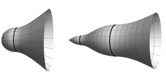
Figure 1: The Hartle-Hawking no-boundary manifold (left) depicts a Euclidean sector glued to the Lorentzian sector at the so-called ’creation surface’. The Vilenkin extension (right) depicts a Euclidean sector sandwiched between two (an embryonic and an eternally expanding) Lorentzian sectors.

Two characterisic features are encountered:

(i) Ironically, while classical cosmology deals by definition with the time evolution of the universe, quantum cosmology is apparently ’static’. What we mean here by ’static’ is merely at the technical level. While classically ${\cal L}(x,\dot{x})$ usually leads to $x(t)$ and quantum mechanically to $\psi(x,t)$, one would naively expect the classical $a(t)$ to be traded quantum mechanically for $\psi(a,t)$ rather than by $\psi(a)$. This indicates that the cosmological wave function does not have any preferred time direction (and most importantly, should not be translated into a static universe). Such an interpretation has initiated a debate regarding both the notion of time Rovelli as well as the arrow of time Kiefer in quantum cosmology.

(ii) Quantum mechanically, for any given scale factor $a$ (not to confuse with classical $a(t)$), spacetime can be either strictly Lorentzian or else strictly Euclidean. The possibility that spacetime is only most probably Lorentzian, a possibility which cannot be a priori ruled out in any quantum gravitational model, is absent.

Harmful pre-gauging

In contrast with the post-gauging option, which is realized at the level of the equations of motion, pre-gauging is carried out already at the level of the Lagrangian. The trouble is that had we pre-gauged the lapse function, pre-fixing for example $n(t)=1$ to start from

$${\cal L}_{1}(a,\dot{a})=a\dot{a}^{2}+a\left(\frac{1}{3}\Lambda a^{2}-k\right)~{},$$ (7)

we would have encountered a major problem since only the 2nd-order Friedmann equation, namely

$$2\frac{\ddot{a}}{a}+\frac{\dot{a}^{2}+k}{a^{2}}=\Lambda~{},$$ (8)

is recovered. A subsequent integration leads to

$$\frac{\dot{a}^{2}+k}{a^{2}}=\frac{1}{3}\Lambda+\frac{E}{a^{3}}~{},$$ (9)

telling us that it is only when the conserved energy $E$ of the system happens to vanish that one correctly recovers the missing 1st-order Friedmann equation. A fake ’dark matter’ component, parametrized by $E$, has entered the game. In other words, over-gauging has killed the Hamiltonian constraint (in charge of enforcing $E=0$). Appreciating this point, the mini Lagrangian eq.(7) cannot be a tenable starting point for a quantum mechanical cosmological model.

While this drawback is generic, there exists a special pre-gauging counter example capable of re-producing the exact classical solution without introducing any fake degree of freedom. We are talking about pre-gauging the scale factor $a(t)$. For example, set $a(t)=t$, giving rise to the mini Lagrangian variant

$${\cal L}_{2}(n,t)=\frac{t}{n}+nt\left(\frac{\Lambda}{3}t^{2}-k\right)~{}.$$ (10)

Counter intuitively, such an unconventional pre-gauging essay does constitute a physically viable option. Indeed, the reduced Euler-Lagrange equation $\displaystyle{\frac{\partial{\cal L}_{2}}{\partial n}=0}$, albeit an algebraic rather than a differential equation, gives rise to the exact solution of the full theory, free of any fake degree of freedom. To be explicit,

$$ds^{2}=-\frac{dt^{2}}{\frac{1}{3}\Lambda t^{2}-k}+t^{2}\left(\frac{dr^{2}}{1-kr^{2}}+r^{2}d\Omega^{2}\right)~{}.$$ (11)

The coefficient of $dt^{2}$ changes sign from $+\infty$ to $-\infty$ (crucially without crossing zero). While the metric is Lorentzian for $t>t_{c}$, it is strikingly Euclidean for $t<t_{c}$. The pole at

$$t_{c}=\sqrt{\frac{3k}{\Lambda}}$$ (12)

deserves some attention. Note that all curvature scalars are non-singular everywhere,

$${\cal R}=-4\Lambda~{},~{}{\cal R}^{\mu\nu}{\cal R}_{\mu\nu}=4\Lambda^{2}~{},~{}{\cal R}^{\mu\nu\lambda\sigma}{\cal R}_{\mu\nu\lambda\sigma}=\frac{8}{3}\Lambda^{2}~{},$$ (13)

including in particular at $t=0$ and at $t=,t_{c}$. This allows for the well known Hartle-Hawking smooth gluing of the Euclidean and the Lorentzian sub-manifolds precisely at $t=t_{c}$ (the manifold is depicted in fig.(1). This point is to be revisited once the lapse function gets slightly modified.

To see things from a different perspective, one may follow Dirac formalism Dirac for dealing with constrained systems. As long as ${\cal L}_{2}(n,t)$ is not a linear function of $n$, the classical equations of motion residing from the corresponding total Hamiltonian serve as consistency checks for the two (a primary and a secondary) second class constraints

$$p_{n}\approx 0~{},\quad\left\{p_{n},{\cal H}_{2}\right\}_{{}_{P}}=\frac{\partial{\cal L}_{2}}{\partial n}\approx 0~{}.$$ (14)

The catch is, however, that starting from ordinary Poisson brackets

$$\left\{n,p_{n}\right\}_{{}_{P}}=1~{},$$ (15)

one ends up with vanishing Dirac brackets

$$\left\{n,p_{n}\right\}_{{}_{D}}=0~{}.$$ (16)

The lesson is clear: Re-producing the exact classical solution is just a necessary condition any mini superspace model must obey. The trouble is that it is not always a sufficient condition as well. As indicated by the vanishing Dirac brackets, the mini superspace model based on the Lagrangian eq.(10) is non-dynamical. While classically this is tolerable, the standard quantization procedure, based on replacing the canonical Dirac brackets by quantum mechanical commutation relations, is blocked. There are cases, however, see the forthcoming dilaton model, where tenable pre-gauging turns harmless, at least in the sense that it leads to a dynamical mini superspace.

Tenable pre-gauging

In search for the missing ingredient, namely a generalized momentum $\tilde{p}_{n}$, Dirac (rather than Poisson) conjugate to the lapse function $n$, we have come across the modified gravity action

$${\cal S}=-\frac{1}{8\pi}\int({\cal R}+4\Lambda)\phi\sqrt{-g}~{}d^{4}x~{},$$ (17)

involving a conformally coupled scalar field $\phi$ (the factor 4 is to be apostriori justified by eq.21). In a somewhat different language, the above prescribes a scale modification $\sqrt{-g}\rightarrow\phi\sqrt{-g}$ of the general relativistic measure. The Kaluza-Klein perspective will be discussed in a forthcoming section.

A few remarks are in order:

(i) One may think of $\phi$ in terms of $\phi=\varphi^{\dagger}\varphi$. In fact, this is a convenient way to explicitly break the classical symmetry $\phi\rightarrow-\phi$ of the field equations, thereby getting rid of the potentially problematic $\phi<0$ anti-gravity GaG regime.

(ii) It should be emphasized that also the current scheme, like the Hartle-Hawking scheme, also has no pretensions to go beyond the scope of a early universe model.

(iii) Reflecting its linearity in the dilaton field, the action eq.(17) has no $f({\cal R})$ analogous theory fR .

(iv) The justification for our modified action comes from the Kaluza-Klein theory. Eq.(17) is nothing but the 4-dim reduction of a 5-dim Einstein-Hilbert action supplemented by a cosmological constant. We later show how the associated 4-dim cosmological evolution, differing from the standard FLRW evolution, is intimately connected with the de-Sitter Kaluza-Klein black hole.

The special dilaton field $\phi(t)$ is accompanied by a linear scalar potential $V(\phi)=4\Lambda\phi$, and is stripped from any Brans-Dicke kinetic term. It is nevertheless a dynamical scalar field as can be verified by extracting its hidden Klein Gordon equation

$$\frac{1}{na^{3}}\frac{d}{dt}\left(\frac{a^{3}}{n}\frac{d\phi}{dt}\right)+V^{\prime}_{eff}(\phi)=0~{},$$ (18)

from the two independent classical equations of motion involved. To be more specific, the time evolution of the dilaton is governed in our case by the effective upside down harmonic potential

$$V_{eff}(\phi)=\frac{1}{3}\int(\phi V^{\prime}-2V)d\phi=-\frac{2}{3}\Lambda\phi^{2}+const~{},$$ (19)

rather than by the original linear potential itself. Note that $\phi=const$ is not a solution. That is to say that the model, at least in its current form, lacks a general relativistic limit. Incorporating a proper general relativistic limit would only require the introduction of a more elaborated effective potential, say $V(\phi)=4\Lambda\phi+\lambda\phi^{2}+\gamma\phi^{3}$, with $16\pi\langle\phi\rangle$ then serving as the reciprocal Newton constant. Such a general relativistic limit is known to be characterized by matter dominated (in average) Hubble constant oscillations averageH . The general relativistic late universe is, however, beyond the scope of our early universe dilaton model (and Hartle-Hawking model as well).

The cosmological evolution, characterized by a constant Ricci scalar ${\cal R}=-4\Lambda$ in the Jordan frame, is then translated Tomer into the equation of state

$$\rho-3P=4\Lambda~{},$$ (20)

which subject to energy/momentum conservation implies

$$\rho=\Lambda+\frac{\xi}{a^{4}}~{},\quad P=-\Lambda+\frac{\xi}{3a^{4}}~{}.$$ (21)

The constant of integration $\xi$ signals the presence of a radiation-like term, the fingerprint of measure scaling. Note that so far, in the literature, radiation has only been introduced ad-hoc Vilenkin into the mini superspace model, inducing (for $\xi>0$) an embryonic universe epoch. Eventually, either recovering from a radiation dominated Big-Bang or else bouncing from a potential hill, the universe glides asymptotically into the de-Sitter phase.

Switching on now the scale factor pre-gauging $a(t)=t$, the mini superspace Lagrangian ${\cal L}_{2}(n,t)$ gets slightly yet significantly modified to read

$${\cal L}(n,\phi,\dot{\phi},t)=\frac{t}{n}(\phi+t\dot{\phi})+nt\left(\frac{2}{3}\Lambda t^{2}-k\right)\phi~{}.$$ (22)

One may verify that the equations of motion derived from this mini Lagrangian give rise to the exact classical solution of the full dilaton gravity theory, namely

$$n^{-2}(t)=\frac{1}{3}\Lambda t^{2}-k+\frac{\xi}{t^{2}}~{},\quad n^{2}(t)\phi^{2}(t)=const~{},$$ (23)

without introducing any fake degree of freedom. If, in addition to the Hartle-Hawking requirements $\Lambda,k>0$, we further require $0<\xi<\frac{3k^{2}}{4\Lambda}$, thereby allowing $n^{-2}(t)=0$ to admit two positive roots $0<t_{-}<t_{+}$. The emerging Euclidean sector associated with $t_{-}<t<t_{+}$ serves as a classical barrier disconnecting a Lorentzian Embryonic universe ($0<t<t_{-}$) from the expanding $\Lambda$-dominated Lorentzian universe ($t_{+}<t<\infty$).

The various curvature scalars eq.(13) are respectively modified to

$${\cal R}=-4\Lambda~{},~{}{\cal R}^{\mu\nu}{\cal R}_{\mu\nu}=4\Lambda^{2}+\frac{12\xi^{2}}{t^{8}}~{},~{}$$

$$\quad{\cal R}^{\mu\nu\lambda\sigma}{\cal R}_{\mu\nu\lambda\sigma}=\frac{8}{3}\Lambda^{2}+\frac{24\xi^{2}}{t^{8}}~{}.$$ (24)

For $\xi\neq 0$, at $t\rightarrow 0$, as expected, the singular Big-Bang event makes its unavoidable appearance. On the other hand, however, the Euclidean to Lorentzian transitions associated with the lapse function pole behavior at

$$t^{2}_{\pm}=\frac{3k}{2\Lambda}\left(1\pm\sqrt{1-\frac{4\Lambda\xi}{3k}}\right)~{},$$ (25)

stay curvature non-singular. This is a crucial point. In the Hartle-Hawking case, $n^{2}(t)<0$ marks a classically forbidden territory. The more so in the present case, where $n^{2}(t)<0$ is further accompanied by $\phi^{2}(t)<0$. In particular, one faces $\phi^{2}(t_{\pm})=0$ at creation. We will re-visit this intriguing $n(t)\leftrightarrow\psi(t)$ sign interplay once the geometrical connection with Kaluza-Klein black hole is established.

The point is that the Lagrangian eq.(22), contrary to the problematic Lagrangian eq.(10), does lead to a dynamical mini superspace (with pre-gauging involved, perhaps a better name is micro-superspace). We proceed now to show how measure scaling combined with scale factor pre-gauging opens the blocked trail to quantum cosmology.

From $\psi(a)$ to $\psi(n,t)$

Within the framework of the Hamiltonian formalism, the fact that one cannot express the ’velocities’ $\dot{n},\dot{\phi}$ in terms of the associated momenta $\displaystyle{p_{n}=\frac{\partial{\cal L}}{\partial\dot{n}}}$ and $\displaystyle{p_{\phi}=\frac{\partial{\cal L}}{\partial\dot{\phi}}}$ results in two primary second class constraints

$$\displaystyle{\chi_{n}\equiv p_{n}\approx 0~{},\quad\chi_{\phi}\equiv p_{\phi}-\frac{t^{2}}{n}\approx 0~{},}$$ (26)

$$\displaystyle{\{\chi_{n},\chi_{\phi}\}_{{}_{P}}=\frac{t^{2}}{n^{2}}~{}.}$$ (27)

Following Dirac prescription, one can keep using the Poisson brackets provided the naive Hamiltonian ${\cal H}$ is traded for the total Hamiltonian

$${\cal H}_{T}={\cal H}+u_{n}\chi_{n}+u_{\phi}\chi_{\phi}~{},$$ (28)

with the two coefficients $u_{1,2}$ fixed on consistency grounds by the requirements

$$\{\chi_{1,2},{\cal H}_{T}\}_{{}_{P}}+\frac{\partial\chi_{1,2}}{\partial t}=0$$ (29)

Alternatively, one may stick to the naive Hamiltonian

$${\cal H}=-\phi t\left[\frac{1}{n}+n\left(\frac{2}{3}\Lambda t^{2}-k\right)\right]~{},$$ (30)

but pay the price of replacing the Poisson brackets by the Dirac brackets. Obviously, only the latter option is relevant for the quantization procedure which is carried out by means of $\{A,B\}_{{}_{D}}=1\rightarrow[A,B]=i\hbar$. With this in mind, we find it now convenient to define a new set of canonical variables

$$x(t)\equiv\frac{t^{2}}{n^{2}(t)}~{},\quad y(t)\equiv\phi^{2}(t)t^{2}~{},$$ (31)

which are introduced of course already at the level of the mini superspace Lagrangian. Such a special $(x,y)$-representation, for which the naive Hamiltonian acquires the compact, notably momentum-free, form

$${\cal H}(x,y,t)=-t\left(\frac{2}{3}\Lambda t^{2}-k\right)\sqrt{\frac{y}{x}}~{},$$ (32)

has been especially designed to remove any explicit time dependence from the various Dirac brackets involved. The crucial observation now is that

$$\{x,y\}_{{}_{P}}=0\quad\Longrightarrow\quad\{x,y\}_{{}_{D}}\neq 0~{},$$ (33)

a fact which has far reaching consequences on the quantization procedure. The WDW wave function cannot depend on $x$ and $y$ simultaneously. To be more specific,

$$\{x,y\}_{{}_{D}}=-4\sqrt{xy}\quad\Longrightarrow\quad\left\{x,-\frac{1}{2}\sqrt{\frac{y}{x}}\right\}_{{}_{D}}=1~{}.$$ (34)

Measure scaling has eventually given birth to a generalized momentum Dirac conjugate to the lapse function. In turn, elevated to the level of a quantum mechanical operator, $\sqrt{y/x}$ can be faithfully represented by

$$\sqrt{\frac{y}{x}}=2i\hbar\frac{\partial}{\partial x}~{}.$$ (35)

Altogether, up to some c-number (reflecting ambiguities arising from operator ordering), the Wheeler-DeWitt Schrodinger equation acquires the atypical linear form

$$-2it\left(\frac{2}{3}\Lambda t^{2}-k\right)\frac{\partial\psi}{\partial x}=i\frac{\partial\psi}{\partial t}~{},$$ (36)

devoid of $\hbar$. Its most general solution is given by

$$\psi(x,t)=\psi(x-\frac{1}{3}\Lambda t^{4}+kt^{2})~{}.$$ (37)

Not only is the WDW wave function $t$-dependent, but it furthermore maintains a constant value, namely $\psi(\xi)$, along the classical path.

One particular solution deserves further attention. We refer of course to the ’most classical’ configuration, namely a Gaussian wave packet wavepacket characterized by the minimal uncertainty relation, explicitly given by

$$\boxed{\psi(x,t)=\frac{e^{\displaystyle{-\frac{\left(x-x_{cl}(t)\right)^{2}}{4\sigma^{2}}+\frac{i\eta}{\sqrt{2}}(x-x_{cl}(t))}}}{(2\pi)^{\frac{1}{4}}\sqrt{\sigma}}}$$ (38)

factorized by an optional linear phase. It is by no means trivial, yet consistent with the correspondence principle (recall the underlying ’most classical’ wave packet), that the most probable as well as the average configuration, is nothing but the classical FLRW solution

$$\langle x\rangle=x_{cl}(t)=\frac{\Lambda}{3}t^{4}-kt^{2}+\xi~{},~{}\langle p_{x}\rangle=\langle-i\hbar\frac{\partial}{\partial x}\rangle=\hbar\eta~{}.$$ (39)

The arbitrary constant $\eta$ matches the classical value of the $n(t)\phi(t)$ product. Note that the uncertainties are time independent

$$\Delta x=\sigma~{},~{}\Delta p_{x}=\frac{\hbar}{2\sigma}~{}.$$ (40)

The cosmological wave packet probability density $|\psi(x,t)|^{2}$ is depicted in Fig.(2). Roughly speaking, we recognize the mainly Euclidean region sandwiched between an optional (for $\xi>0$) mainly Lorentzian Vilenkin-type embryonic era (on the lhs) and the asymptotically classical mainly Lorentzian region (on the rhs). As a consistency check one may verify that the probability $P(t)$ that spacetime is Lorentzian approaches unity as $t\rightarrow\infty$. To be specific,

$$\boxed{P(t)=\int_{0}^{\infty}|\psi(x,t)|^{2}dx\simeq 1-\frac{3\sigma}{\sqrt{2\pi}\Lambda t^{4}}e^{\displaystyle{-\frac{\Lambda^{2}t^{8}}{18\sigma^{2}}}}}$$ (41)

At this point, noticing that eq.(36) is $\hbar$-independent, one may wonder where is the Planck scale hiding? On dimensional grounds, it can only enter the game via the spread parameter $\sigma$. In fact, as it has been argued, see ref.area , based on micro black hole thermodynamics arguments (the behavior of the entropy and the Helmholtz free energy as functions of the Hawking temperature), one may expect $\sigma\simeq\ell_{Planck}\sim\sqrt{\hbar}$. This would assure us that a Euclide $\leftrightarrow$ Lorentz transition is highly improbable at large $t$. At short $t$, on the other hand, the quantum mechanically smeared Lorentz $\leftrightarrow$ Euclid interplay takes over. Even the naive question ’when has creation occurred?’ can only be answered statistically. This may be connected to the general idea of the multiverse. The no-boundary proposal limit, if exists, is still hidden at this stage.

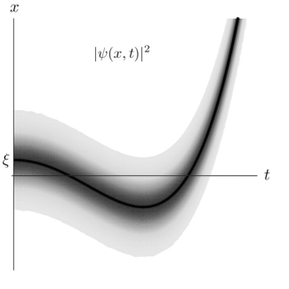
Figure 2: Cosmological wave packet probability density: For any time $t$, unlike in the Hartle-Hawking scheme, there is a probability that spacetime is Lorentzian ($x>0$) and a complementary probability that it is Euclidean ($x<0$). The sharp Euclidean to Lorentzian regime crossover ($\equiv$ creation) has been quantum mechanically smeared.

The Kaluza-Klein black hole connection

Importing the classical solution eq.(23) previously derived into a 5-dimensional world (with a 3-dimensional maximally symmetric subspace imposed), we face the line element

$$ds^{2}_{5}=-n^{2}(t)dt^{2}+t^{2}\left(\frac{d\rho^{2}}{1-k\rho^{2}}+\rho^{2}d\Omega^{2}\right)+\phi^{2}(t)dx^{2}_{5}~{}.$$ (42)

For the sake of definiteness, let us momentarily assume $\Lambda,k>0$ to keep track with the Hartle-Hawking scheme, and thereby encounter the familiar $x_{5}$-independent (a la Kaluza-Klein by virtue of Birkhoff theorem) general relativistic Schwarzschild-deSitter black hole metric in disguise. The standard form is met by simply replacing the notations according to

$$t\rightarrow r,~{}x_{5}\rightarrow t~{},$$ (43)

accompanied by the (mass)² identification $\xi=m^{2}$. Altogether, this establishes an intriguing analogy between the 4-dimensional $t$-dependent quantum cosmology and the 5-dimensional $\rho$-dependent black hole. In particular, the Euclidean $\leftrightarrow$ Lorentzian transition at $t=t_{+}$, referred to as the creation surface in the 4-dim language, is recognized as the outer horizon of the Schwarzschild-de-Sitter Kaluza-Klein black hole. This is of course not a coincidence. By substituting the 5-dim metric ansatz eq.(42) into the Kaluza-Klein action

$${\cal S}_{5}=-\frac{1}{4\pi}\int\left({\cal R}_{5}+4\Lambda\right)\sqrt{-g_{5}}~{}d^{5}x~{},$$ (44)

and integrating out the $S_{3}$ sub-manifold as well as the $x_{5}$-circle, one encounters (up to a total derivative) the one and the same mini superspace Lagrangian eq.(22).

With this in mind we note that the quantum mechanical 4-dim Schwarzschild black hole has already been discussed in the midi-superspace model Kuchar , in the Dirac style pre-gauging formalism area , and in the technical context of a generalized uncertainty principle Casadio . The ’most classical’ non-singular circumferential radius $r$-dependent Schwarzschild black hole wave packet is given by

$$\psi_{BH}(x,r)=\frac{1}{(2\pi)^{\frac{1}{4}}\sqrt{\sigma}}e^{-\displaystyle{\frac{\left(x-2r+4m\right)^{2}}{4\sigma^{2}}}}~{}.$$ (45)

A linear phase is optional. Up to an $r\leftrightarrow t$ role interchange, eq.(45) highly resembles eq.(38). In particular, the variable $x$ which has played the role of $-t^{2}/g_{tt}$ in the our cosmological scheme, stands here for $2r/g_{rr}$. The dictionary continuous as follows. The analog of the mass parameter $m$ is clearly the amount $\xi$ of cosmological radiation. Likewise, the analog of the classical black hole event horizon (at $r=2m$) is the so-called creation surface (at $t=t_{c}$) on which $n^{-2}(t_{c})$ happens to vanish. Carrying the analogy one step further, the cosmological (black hole) wave packet probability density $\psi^{\dagger}\psi$ can be effectively translated into a statistical mechanics radiation (mass) spectrum.

Summary table

To summarize, here is a compact table emphasizing the main differences between the standard Hartle-Hawking mini superspace approach and our measure scaling dilatonic (Kaluza-Klein originated) variant:

$$\begin{array}[]{c|c|c}&\text{HH model}&\text{This model}\\ \hline\cr\text{Wave function}&t\text{--independent}&t\text{--dependent}\\ \hline\cr\text{Classical solution}&\text{QM irrelevant}&\text{QM relevant}\\ \hline\cr\text{Black Hole analogy}&\text{No}&\text{Yes (5-dim)}\\ \hline\cr\text{Euclid/Lorentz crossover}&\text{Sharp}&\text{Smeared}\end{array}$$

A mini superspace model can never replace the full theory. This is true for the Hartle-Hawking mini superspace model, and holds of course for the present micro superspace model as well. It can at most give us a clue what to expect when quantum gravity will eventually make its appearance. And once gravity meets the quantum world (going beyond the level of various mini superspace models), the idea that spacetime is just most probably Lorentzian seems quite natural and in some respect even unavoidable. As far as we can tell, such an idea has never been put forwards. While the complementary probability that spacetime is Euclidean must be vanishingly small today, it could have had interesting consequences at the very early universe owing to the quantum mechanical smearing of the Euclid/Lorentz crossover.

- (1) B.S. DeWitt, Phys. Rev. 160, 1113 (1967); J.A. Wheeler, in Battelle Rencontres, 242 (Benjamin NY, 1968); C.W. Misner, Phys. Rev. 186, 1319 (1969).
- (2) K.V. Kuchar and M.P. Ryan, Phys. Rev. D40, 3982 (1989); S. Sinha and B.L. Hu, Phys. Rev. D44, 1028 (1991).
- (3) M. Bojowald, Rep. Prog. Phys. 78, 023901 (2015).
- (4) J.B. Hartle and S W. Hawking, Phys. Rev. D28, 2960 (1983); A.D. Linde, Nuovo Cimento 39, 401 (1984);
- (5) A. Vilenkin, Phys. Rev. D30, 509 (1984); A. Vilenkin, Phys. Rev. D37, 888 (1988); A. Vilenkin, Phys. Rev. D50 2581 (1994).
- (6) C. Rovelli, Phys. Rev. D42, 2638 (1990); ibid, Phys. Rev. D43, 442 (1991).
- (7) ”The arrows of time - a debate in cosmology”, L. Mersini-Houghton and R. Vass editors, (Springer-Verlag 2012); C. Kiefer, Fundamental Theories of Physics 172, 191 (2011).
- (8) A. Davidson and B. Yellin, Int. Jour. Mod. Phys. D21, 1242011 (2012).
- (9) P.A.M. Dirac, in Lectures on quantum mechanics, (Dover publications, 1964); ibid. Canad. Jour. Math. 2, 129 (1950).
- (10) I. Bars, S.H. Chen, P.J. Steinhardt and N. Turok, Phys. Lett. B715, 278 (2012); I. Bars, P. Steinhardt and N. Turok, Phys. Rev. D89, 061302(R) (2014); K. Bamba, S. Nojiri, S.D. Odintsov and D. Saez-Gomez, Phys. Lett. 730, 136 (2014); J. Joseph, M. Carrasco, W. Chemissany and R. Kallosh, JHEP 1401, 130 (2014).
- (11) A. Davidson, Class. Quant. Grav. 22, 1119 (2005).
- (12) T.P. Sotiriou and V. Faraoni, Rev. Mod. Phys. 82, 451 (2010); B. Vakili, Ann. Phys. 19, 359 (2010); A, De Felice and S. Tsujikawa, Living Rev. Rel. 13, 3 (2010); S. Nojiri and S.D. Odintsov, Phys. Rep. 505, 59 (2011); T. Clifton, P.G. Ferreira, A. Padilla, and C. Skordis, Phys. Rep. 513, 1 (2012).
- (13) A. Davidson and T. Igael, Class. Quant. Grav. 32, 152001 (2015).
- (14) A. Vilenkin, AIP Conf. Proc. 478, 23 (1999); A. Davidson, D. Karasik and Y. Lederer, Class. Quant. Grav. 166, 1349 (1999); A. Vilenkin, Conf. C02-01-07.7 Proc., 649 (2002); R. Cordero and A. Vilenkin, Phys. Rev. D65, 083519 (2002).
- (15) C. Kiefer, Phys. Rev. D38, 1761 (1988).
- (16) K.V. Kuchar, Phys. Rev. D50, 3961 (1994); T. Brotz and C. Kiefer, Phys. Rev. D55, 2186 (1997).
- (17) A. Davidson and B. Yellin, Phys. Lett. B736, 267 (2014).
- (18) R Casadio, F Scardigli, Euro. Phys. Jour. C74, 2685 (2014).